Diffusion and robustness of boundary feedback stabilization of hyperbolic systems
À notre maitre et ami Eduardo

Georges Bastin  ,  Jean-Michel Coron   and Amaury Hayat Department of Mathematical Engineering, ICTEAM, UCLouvain, Louvain-La-Neuve, Belgium. georges.bastin@uclouvain.beLaboratoire Jacques-Louis Lions, Sorbonne Université, Université de Paris, CNRS, INRIA, équipe Cage, Paris, France. jean-michel.coron@sorbonne-universite.frCERMICS, École des Ponts ParisTech, 6 - 8, Avenue Blaise Pascal, Cité Descartes - Champs sur Marne, 77455 Marne la Vallée, France. amaury.hayat@enpc.fr.
Abstract

We consider the problem of boundary feedback control of single-input-single-output (SISO) one-dimensional linear hyperbolic systems when sensing and actuation are anti-located. The main issue of the output feedback stabilization is that it requires dynamic control laws that include delayed values of the output (directly or through state observers) which may not be robust to infinitesimal uncertainties on the characteristic velocities. The purpose of this paper is to highlight some features of this problem by addressing the feedback stabilization of an unstable open-loop system which is made up of two interconnected transport equations and provided with anti-located boundary sensing and actuation. The main contribution is to show that the robustness of the control against delay uncertainties is recovered as soon as an arbitrary small diffusion is present in the system. Our analysis also reveals that the effect of diffusion on stability is far from being an obvious issue by exhibiting an alternative simple example where the presence of diffusion has a destabilizing effect instead.

1 Introduction

The output feedback stabilization of single-input-single-output (SISO) one-dimensional linear hyperbolic systems is a subject that has been widely studied in the scientific literature since the nineties when both actuation and sensing are located at the boundaries. In the case where the control input and the measured output are co-located at the same boundary, the problem is now relatively well understood and has given rise to numerous publications, both in the linear case [1, 3] and in the nonlinear case [5, 13], in particular in fluid mechanics for Saint-Venant equations [10, 5, 16] or Euler equations [14], to name just a few of the many publications on the subject.

In contrast, when the actuator acts through one boundary, whereas the sensor is placed at the other boundary, the output feedback stabilization problem can become much more complicated and remains largely unexplored in the literature. As Krstic et al. pointed out in [18], the difficulty arises from the fact that “the input-output operator is no longer passive (…) which precludes the application of simple controllers”. Anti-located sensing and actuation requires to use dynamic compensators that include delayed values of the output (directly or through state observers). A meaningful example is the output feedback stabilization of a simple unstable wave equation addressed in [18] using a separation principle that combines a state feedback control with a state observer. This approach is extended to the adaptive stabilization of more general linear hyperbolic systems with unknown parameters in [2] and [7]. Recently, an experimental application to the control of hydraulic waves is reported in [23], where the actuation is provided by a moving boundary while the water level is measured at the other boundary.

We can also mention references [4, 17] which deal with MIMO systems with anti-located multivariable sensors and actuators for n×n𝑛𝑛n\times n linear hyperbolic systems expressed in a characteristic form having a very specific input/output structure.

It is important to note that the use of control laws containing delayed output feedback or state observers can however prove to be problematic because it can be strongly sensitive to uncertainties on the characteristic velocities of the plant model [20, 12, 8]. This happens when the control design relies on a (supposed) exact knowledge of some characteristic velocities that must be exactly compensated in the control law such that the stability can be destroyed by arbitrarily small modelling uncertainties.

In this paper, our purpose is to highlight some features of this problem by addressing the feedback stabilization of an unstable open-loop system which is made up of two interconnected transport equations and provided with anti-located boundary sensing and actuation.

Our paper is organized as follows. The control problem is described in Section 2. It is first shown that the considered control system is open loop unstable and cannot be stabilized by a simple proportional output feedback. Then, it is shown that the system can be stabilized by a dynamic controller that involves a delayed output feedback. However, this control turns out not to be robust with respect to delay uncertainties precisely because the control requires a (utopian) exact knowledge of the transport velocity.

The main contribution of this paper is to show that the robustness of the control against delay uncertainties is recovered as soon as an arbitrary small diffusion is present in the system. For that purpose, in Section 3, it is first assumed that the considered plant is subject to a slight phenomenon of diffusion, interpreted as a viscosity and the corresponding (unstable) input-output transfer function is computed. Then in Sections 4 and 5, we show that the dynamic output (non robust) feedback designed for the inviscid case also stabilizes exponentially the viscous system when the (unknown) diffusion is small, and that, in this case, the control proves to be perfectly robust, even if the diffusion is almost negligible. Interestingly, an upper bound on the decay rate appears when adding a small viscosity, and this upper bound is uniform with respect to the diffusion parameter η𝜂\eta when it is small, while for the unperturbed system with η=0𝜂0\eta=0 the decay rate is infinite (the system is finite-time stable).

Our analysis in Sections 4 and 5 also reveals that the effect of diffusion on stability is far from being an obvious issue, contrary to what one might expect. It is indeed well known that, in hyperbolic systems, the presence of diffusion (or friction) can have a destabilizing as well as a stabilizing effect (see for instance the references [11, 22]). This issue is further discussed in Section 6 where we present an example of another simple hyperbolic system which simplifies the previous case and for which, however, the same diffusion term destroys the stability instead of strengthening it.

Some final conclusions are given in Section 7.

2 Description of the control problem

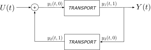
We consider the open loop control system represented in Figure 1. The system is made up of the positive feedback interconnection of two identical transport systems. The system dynamics are described in the time domain by the following equations:

ty1(t,x)+υxy1(t,x)=0,subscript𝑡subscript𝑦1𝑡𝑥𝜐subscript𝑥subscript𝑦1𝑡𝑥0\displaystyle\partial_{t}y_{1}(t,x)+\upsilon\partial_{x}y_{1}(t,x)=0, (1a)
ty2(t,x)+υxy2(t,x)=0,subscript𝑡subscript𝑦2𝑡𝑥𝜐subscript𝑥subscript𝑦2𝑡𝑥0\displaystyle\partial_{t}y_{2}(t,x)+\upsilon\partial_{x}y_{2}(t,x)=0, (1b)
y1(t,0)=y2(t,1)+U(t),subscript𝑦1𝑡0subscript𝑦2𝑡1𝑈𝑡\displaystyle y_{1}(t,0)=y_{2}(t,1)+U(t), (1c)
y2(t,0)=y1(t,1),subscript𝑦2𝑡0subscript𝑦1𝑡1\displaystyle y_{2}(t,0)=y_{1}(t,1), (1d)
Y(t)=y1(t,1).𝑌𝑡subscript𝑦1𝑡1\displaystyle Y(t)=y_{1}(t,1). (1e)

where U(t)𝑈𝑡U(t) is the control input and Y(t)𝑌𝑡Y(t) is the measurable output. In the classical pure transport equations (1a) and (1b), the parameter υ>0𝜐0\upsilon>0 denotes the transport velocity.

Refer to caption
Figure 1: The structure of the open loop control system considered in this paper.

In the frequency domain, it is well known that the transfer function of the transport systems (1a) and (1b) is

fo(s)=esτwith the time delayτ=1υ,formulae-sequencesubscript𝑓𝑜𝑠superscript𝑒𝑠𝜏with the time delay𝜏1𝜐f_{o}(s)=e^{-s\tau}\hskip 14.22636pt\text{with the time delay}\hskip 14.22636pt\tau=\dfrac{1}{\upsilon}, (2)

where s𝑠s denotes the Laplace complex variable.

It follows that the overall input-output transfer function of the open loop system (1) is

G(s)=Y(s)U(s)=fo(s)1fo2(s)=esτe2sτ1,𝐺𝑠Y𝑠U𝑠subscript𝑓𝑜𝑠1superscriptsubscript𝑓𝑜2𝑠superscript𝑒𝑠𝜏superscript𝑒2𝑠𝜏1G(s)=\dfrac{\textrm{Y}(s)}{\textrm{U}(s)}=\dfrac{f_{o}(s)}{1-f_{o}^{2}(s)}=\dfrac{e^{s\tau}}{e^{2s\tau}-1}, (3)

where Y(s)Y𝑠\textrm{Y}(s) and U(s)U𝑠\textrm{U}(s) denote the Laplace transforms of the output Y(t)𝑌𝑡Y(t) and the input U(t)𝑈𝑡U(t) respectively.

The poles of the system are the roots of the characteristic equation

e2sτ1=0.superscript𝑒2𝑠𝜏10e^{2s\tau}-1=0. (4)

This open loop control system is clearly not asymptotically stable since all the poles are located on the imaginary axis.

In order to illustrate the challenge that arises when actuation and sensing are anti-located, we shall first show that, despite its apparent simplicity, this unstable system cannot be stabilized with a simple proportional output feedback, i.e. with a static proportional controller of the form

U(t)=2kpY(t)𝑈𝑡2subscript𝑘𝑝𝑌𝑡U(t)=-2k_{p}Y(t) (5)

where kp0subscript𝑘𝑝0k_{p}\neq 0 is a control tuning parameter.

In the frequency domain, for the system (3) with the control law (5) the characteristic equation of the closed loop system is:

e2sτ+2kpesτ1=0.superscript𝑒2𝑠𝜏2subscript𝑘𝑝superscript𝑒𝑠𝜏10e^{2s\tau}+2k_{p}e^{s\tau}-1=0. (6)

Solving this equation for esτsuperscript𝑒𝑠𝜏e^{s\tau}, we get

esτ=kp±1+kp2.superscript𝑒𝑠𝜏plus-or-minussubscript𝑘𝑝1superscriptsubscript𝑘𝑝2e^{s\tau}=-k_{p}\pm\sqrt{1+k_{p}^{2}}. (7)

Then for any kp0subscript𝑘𝑝0k_{p}\neq 0 there is an infinity of system poles σ+iω𝜎𝑖𝜔\sigma+i\omega lying on two vertical lines with real parts:

σ=υln(1+kp2+|kp|)>0andσ=υln(1+kp2|kp|)<0.formulae-sequence𝜎𝜐1superscriptsubscript𝑘𝑝2subscript𝑘𝑝0and𝜎𝜐1superscriptsubscript𝑘𝑝2subscript𝑘𝑝0\sigma=\upsilon\ln\left(\sqrt{1+k_{p}^{2}}+|k_{p}|\right)>0\hskip 14.22636pt\text{and}\hskip 14.22636pt\sigma=\upsilon\ln\left(\sqrt{1+k_{p}^{2}}-|k_{p}|\right)<0. (8)

It follows that the unstable system (3) cannot be stabilized with the static controller (5).

Let us now show that the system can actually be stabilized by a dynamic controller that involves a delayed output feedback.

From (3), it follows that the input-output dynamics of the system (1) in the time domain can alternatively be represented by the delay-difference equation

Y(t)Y(t2τ)=U(tτ).𝑌𝑡𝑌𝑡2𝜏𝑈𝑡𝜏Y(t)-Y(t-2\tau)=U(t-\tau). (9)

A simple and natural candidate for a stabilizing feedback control law is then

U(t)=2k1Y(t)k2Y(tτ)𝑈𝑡2subscript𝑘1𝑌𝑡subscript𝑘2𝑌𝑡𝜏U(t)=-2k_{1}Y(t)-k_{2}Y(t-\tau) (10)

where k1subscript𝑘1k_{1} and k2subscript𝑘2k_{2} are control tuning parameters. With this control law, the closed loop dynamics are

Y(t)+2k1Y(tτ)+(k21)Y(t2τ)=0.𝑌𝑡2subscript𝑘1𝑌𝑡𝜏subscript𝑘21𝑌𝑡2𝜏0Y(t)+2k_{1}Y(t-\tau)+(k_{2}-1)Y(t-2\tau)=0. (11)

Clearly, we can conclude that the controller (10) exponentially stabilizes the system (1) if the tuning parameters k1subscript𝑘1k_{1} and k2subscript𝑘2k_{2} are selected such that the roots of the polynomial

w2+2k1w+(k21)superscript𝑤22subscript𝑘1𝑤subscript𝑘21w^{2}+2k_{1}w+(k_{2}-1) (12)

are located inside the unit circle. However, this should be considered with caution because it is well known that boundary feedback stabilization of hyperbolic systems with delayed control may be sensitive to delay modeling errors (see e.g. [20]). To clarify this point we consider the time domain representation of the dynamical control law (10) defined as

ty^2(t,x)+υxy^2(t,x)=0,y^2(t,0)=y1(t,1),formulae-sequencesubscript𝑡subscript^𝑦2𝑡𝑥𝜐subscript𝑥subscript^𝑦2𝑡𝑥0subscript^𝑦2𝑡0subscript𝑦1𝑡1\displaystyle\begin{split}&\partial_{t}\hat{y}_{2}(t,x)+\upsilon\partial_{x}\hat{y}_{2}(t,x)=0,\\ &\hat{y}_{2}(t,0)=y_{1}(t,1),\end{split} (13)
U(t)=2k1y1(t,1)k2y^2(t,1),𝑈𝑡2subscript𝑘1subscript𝑦1𝑡1subscript𝑘2subscript^𝑦2𝑡1\displaystyle U(t)=-2k_{1}y_{1}(t,1)-k_{2}\hat{y}_{2}(t,1), (14)

where the transport equation (13) with transport velocity υ=1/τ𝜐1𝜏\upsilon=1/\tau is equivalent to the time delay τ𝜏\tau of the control law (10). With this definition, the closed loop system (1), (13), (14) is then represented as follows:

ty1(t,x)+υxy1(t,x)=0,subscript𝑡subscript𝑦1𝑡𝑥𝜐subscript𝑥subscript𝑦1𝑡𝑥0\displaystyle\partial_{t}y_{1}(t,x)+\upsilon\partial_{x}y_{1}(t,x)=0, (15a)
ty2(t,x)+υxy2(t,x)=0,subscript𝑡subscript𝑦2𝑡𝑥𝜐subscript𝑥subscript𝑦2𝑡𝑥0\displaystyle\partial_{t}y_{2}(t,x)+\upsilon\partial_{x}y_{2}(t,x)=0, (15b)
ty^2(t,x)+υxy^2(t,x)=0,subscript𝑡subscript^𝑦2𝑡𝑥𝜐subscript𝑥subscript^𝑦2𝑡𝑥0\displaystyle\partial_{t}\hat{y}_{2}(t,x)+\upsilon\partial_{x}\hat{y}_{2}(t,x)=0, (15c)
(y1(t,0)y2(t,0)y^2(t,0))=(2k11k2100 100)𝐊(y1(t,1)y2(t,1)y^2(t,1)).matrixsubscript𝑦1𝑡0subscript𝑦2𝑡0subscript^𝑦2𝑡0subscriptmatrix2subscript𝑘11subscript𝑘2100100𝐊matrixsubscript𝑦1𝑡1subscript𝑦2𝑡1subscript^𝑦2𝑡1\displaystyle\begin{pmatrix}y_{1}(t,0)\\[5.0pt] y_{2}(t,0)\\[5.0pt] \hat{y}_{2}(t,0)\end{pmatrix}=\underbrace{\begin{pmatrix}-2k_{1}&1&-k_{2}\\[5.0pt] 1&0&0\\[5.0pt] \ 1&0&0\end{pmatrix}}_{\displaystyle\mathbf{K}}\begin{pmatrix}y_{1}(t,1)\\[5.0pt] y_{2}(t,1)\\[5.0pt] \hat{y}_{2}(t,1)\end{pmatrix}. (15d)

Now, as proved in Appendix A, for the matrix 𝐊𝐊\mathbf{K} defined in (15d), it can be shown that

ρ¯(𝐊)=|k1|+1+k12+|k2|1for all (k1,k2)2,formulae-sequence¯𝜌𝐊subscript𝑘11superscriptsubscript𝑘12subscript𝑘21for all subscript𝑘1subscript𝑘2superscript2\bar{\rho}(\mathbf{K})=|k_{1}|+\sqrt{1+k_{1}^{2}+|k_{2}|}\;\geqslant 1\hskip 14.22636pt\text{for all }(k_{1},k_{2})\in\mathbb{R}^{2}, (16)

where ρ¯(𝐊)¯𝜌𝐊\bar{\rho}(\mathbf{K}) is defined as follows:

ρ¯(𝐊):=max{ρ(diag{eiθ1,eiθ2,eiθ3}𝐊);(θ1,θ2,θ3)𝖳3},assign¯𝜌𝐊𝜌diagsuperscript𝑒𝑖subscript𝜃1superscript𝑒𝑖subscript𝜃2superscript𝑒𝑖subscript𝜃3𝐊superscriptsubscript𝜃1subscript𝜃2subscript𝜃3𝖳superscript3\bar{\rho}(\mathbf{K}):=\max\{\rho(\text{diag}\!\left\{e^{-i\theta_{1}},e^{-i\theta_{2}},e^{-i\theta_{3}}\right\}\mathbf{K});(\theta_{1},\theta_{2},\theta_{3})^{\!\mathsf{T}}\in\mathbb{R}^{3}\}, (17)

ρ(M)𝜌𝑀\rho(M) denoting the spectral radius of the matrix M𝑀M. By [21] (see also [15, Chapter 9, Theorem 6.1] and [5, Chapter 3]), we know that ρ¯(𝐊)<1¯𝜌𝐊1\bar{\rho}(\mathbf{K})<1 is a necessary (and sufficient) condition to have a stability which is robust against small uncertainties in the characteristic velocities. Although the ideal closed loop system (15) is exponentially stable (with all the poles strictly located in the left half complex plane provided k1subscript𝑘1k_{1} and k2subscript𝑘2k_{2} are chosen accordingly), the stability can be destroyed by an arbitrarily small difference in characteristic velocities between the plant equations (15a), (15b) and the controller equation (15c). More precisely, if we assume that the physical transport velocities are υ+ε1𝜐subscript𝜀1\upsilon+\varepsilon_{1}, υ+ε2𝜐subscript𝜀2\upsilon+\varepsilon_{2} with ε1,ε2subscript𝜀1subscript𝜀2\varepsilon_{1},\varepsilon_{2} representing uncertainties in the plant equations (15a), (15b) rewritten as follows:

ty1(t,x)+(υ+ε1)xy1(t,x)=0,subscript𝑡subscript𝑦1𝑡𝑥𝜐subscript𝜀1subscript𝑥subscript𝑦1𝑡𝑥0\displaystyle\partial_{t}y_{1}(t,x)+(\upsilon+\varepsilon_{1})\partial_{x}y_{1}(t,x)=0, (18a)
ty2(t,x)+(υ+ε2)xy2(t,x)=0,subscript𝑡subscript𝑦2𝑡𝑥𝜐subscript𝜀2subscript𝑥subscript𝑦2𝑡𝑥0\displaystyle\partial_{t}y_{2}(t,x)+(\upsilon+\varepsilon_{2})\partial_{x}y_{2}(t,x)=0, (18b)

then the closed loop system (15) with (15a), (15b) replaced by (18a), (18b) may become unstable, with poles moving to the right half complex plane even for arbitrarily small εisubscript𝜀𝑖\varepsilon_{i} perturbations.

Should this necessarily mean that the control law (10) with delayed feedback could not be applied in practice? Our objective, in this paper, is exactly to prove the opposite! Indeed, our main contribution will be to show that, even with the simple control law (10), the robustness of the output feedback stabilization against delay uncertainties can be recovered as soon as an arbitrary small diffusion is present in the system. Our analysis will also reveal, however, that the effect on stability of adding an arbitrarily small diffusion is far from obvious, contrary to what one might expect. Indeed, while diffusion strengthens the robustness of the exponential stability for the 2×2222\times 2 problem (18), it can also destroy the stability of similar simpler systems as we will see in Section 6.

We shall consider the special case of a dead beat control where k1=0subscript𝑘10k_{1}=0 and k2=1subscript𝑘21k_{2}=1. In that case the characteristic equation of the closed loop inviscid system reduces to e2sτ=0superscript𝑒2𝑠𝜏0e^{2s\tau}=0, meaning that all the poles of the system have negative real parts that are moved off to infinity. However, for that system we have

ρ¯(𝐊)=2¯𝜌𝐊2\bar{\rho}(\mathbf{K})=\sqrt{2} (19)

showing a strict lack of robustness of the control w.r.t. delay inaccuracy.

3 The open loop control system with diffusion

We consider again a control system as represented in Figure 1. However, we assume here that the two transport systems are subject to a slight phenomenon of diffusion. The system is therefore made up of the feedback interconnection of two identical transport systems that are perturbed by a diffusion term which can be interpreted for example as a viscosity in the case of a fluid. For simplicity and without loss of generality, we assume a unit nominal transport velocity υ=1𝜐1\upsilon=1. The dynamics of the open loop control system are therefore described in the time domain by the following equations:

ty1(t,x)+xy1(t,x)ηxx2y1(t,x)=0,subscript𝑡subscript𝑦1𝑡𝑥subscript𝑥subscript𝑦1𝑡𝑥𝜂subscriptsuperscript2𝑥𝑥subscript𝑦1𝑡𝑥0\displaystyle\partial_{t}y_{1}(t,x)+\partial_{x}y_{1}(t,x)-\eta\partial^{2}_{xx}y_{1}(t,x)=0, (20a)
ty2(t,x)+xy2(t,x)ηxx2y2(t,x)=0,subscript𝑡subscript𝑦2𝑡𝑥subscript𝑥subscript𝑦2𝑡𝑥𝜂subscriptsuperscript2𝑥𝑥subscript𝑦2𝑡𝑥0\displaystyle\partial_{t}y_{2}(t,x)+\partial_{x}y_{2}(t,x)-\eta\partial^{2}_{xx}y_{2}(t,x)=0, (20b)
y1(t,0)=y2(t,1)+U(t),subscript𝑦1𝑡0subscript𝑦2𝑡1𝑈𝑡\displaystyle y_{1}(t,0)=y_{2}(t,1)+U(t), (20c)
y2(t,0)=y1(t,1),subscript𝑦2𝑡0subscript𝑦1𝑡1\displaystyle y_{2}(t,0)=y_{1}(t,1), (20d)
xy1(t,1)=xy2(t,1)=0subscript𝑥subscript𝑦1𝑡1subscript𝑥subscript𝑦2𝑡10\displaystyle\partial_{x}y_{1}(t,1)=\partial_{x}y_{2}(t,1)=0 (20e)
Y(t)=y1(t,1).𝑌𝑡subscript𝑦1𝑡1\displaystyle Y(t)=y_{1}(t,1). (20f)

As above U(t)𝑈𝑡U(t) is the control input and Y(t)𝑌𝑡Y(t) is the measurable output while η>0𝜂0\eta>0 is the viscosity coefficient.

In the frequency domain, with y1(s,x)subscripty1𝑠𝑥\textrm{y}_{\!1}(s,x) and y2(s,x)subscripty2𝑠𝑥\textrm{y}_{2}(s,x) denoting the Laplace transforms of y1(t,x)subscript𝑦1𝑡𝑥y_{1}(t,x) and y2(t,x)subscript𝑦2𝑡𝑥y_{2}(t,x), the system is written

sy1(s,x)+xy1(s,x)ηxx2y1(s,x)=0,𝑠subscripty1𝑠𝑥subscript𝑥subscripty1𝑠𝑥𝜂subscriptsuperscript2𝑥𝑥subscripty1𝑠𝑥0\displaystyle s\textrm{y}_{\!1}(s,x)+\partial_{x}\textrm{y}_{\!1}(s,x)-\eta\partial^{2}_{xx}\textrm{y}_{\!1}(s,x)=0, (21a)
sy2(s,x)+xy2(s,x)ηxx2y2(s,x)=0,𝑠subscripty2𝑠𝑥subscript𝑥subscripty2𝑠𝑥𝜂subscriptsuperscript2𝑥𝑥subscripty2𝑠𝑥0\displaystyle s\textrm{y}_{2}(s,x)+\partial_{x}\textrm{y}_{2}(s,x)-\eta\partial^{2}_{xx}\textrm{y}_{2}(s,x)=0, (21b)
y1(s,0)=y2(s,1)+U(s),subscripty1𝑠0subscripty2𝑠1U𝑠\displaystyle\textrm{y}_{\!1}(s,0)=\textrm{y}_{2}(s,1)+\textrm{U}(s), (21c)
y2(s,0)=y1(s,1),subscripty2𝑠0subscripty1𝑠1\displaystyle\textrm{y}_{2}(s,0)=\textrm{y}_{\!1}(s,1), (21d)
xy1(s,1)=xy2(s,1)=0subscript𝑥subscripty1𝑠1subscript𝑥subscripty2𝑠10\displaystyle\partial_{x}\textrm{y}_{\!1}(s,1)=\partial_{x}\textrm{y}_{2}(s,1)=0 (21e)
Y(s)=y1(s,1).Y𝑠subscripty1𝑠1\displaystyle\textrm{Y}(s)=\textrm{y}_{\!1}(s,1). (21f)

For any value of s, the solutions of the differential equations (21a), (21b) are written

yi(s,x)=Ai(s)eλ1(s)x+Bi(s)eλ2(s)x,i=1,2,formulae-sequencesubscripty𝑖𝑠𝑥subscript𝐴𝑖𝑠superscript𝑒subscript𝜆1𝑠𝑥subscript𝐵𝑖𝑠superscript𝑒subscript𝜆2𝑠𝑥𝑖12\textrm{y}_{i}(s,x)=A_{i}(s)e^{\lambda_{1}(s)x}+B_{i}(s)e^{\lambda_{2}(s)x},\hskip 14.22636pti=1,2, (22)

where λ1(s)subscript𝜆1𝑠\lambda_{1}(s), λ2(s)subscript𝜆2𝑠\lambda_{2}(s) are the roots of the polynomial

ηλ2λs=0,𝜂superscript𝜆2𝜆𝑠0\eta\lambda^{2}-\lambda-s=0, (23)

which implies that

λ1(s)=1+1+4ηs2η,λ2(s)=11+4ηs2η.formulae-sequencesubscript𝜆1𝑠114𝜂𝑠2𝜂subscript𝜆2𝑠114𝜂𝑠2𝜂\lambda_{1}(s)=\dfrac{1+\sqrt{1+4\eta s}}{2\eta},\hskip 14.22636pt\lambda_{2}(s)=\dfrac{1-\sqrt{1+4\eta s}}{2\eta}. (24)

In (24) and in the following \sqrt{\cdot} denotes the principal value of the square root, which is well defined except when 1+4ηs14𝜂𝑠subscript1+4\eta s\in\mathbb{R}_{-}; however this particular case implies that s𝑠s is real and s1/4η𝑠14𝜂s\leq-1/4\eta and therefore is negative and converges to -\infty when η0+𝜂superscript0\eta\rightarrow 0^{+}. We will see later on that this case can be considered separately. Using the solution (22) and the boundary condition (21e), we have for each i=1,2𝑖12i=1,2,

Ai(s)+Bi(s)=yi(s,0),subscript𝐴𝑖𝑠subscript𝐵𝑖𝑠subscripty𝑖𝑠0\displaystyle A_{i}(s)+B_{i}(s)=\textrm{y}_{i}(s,0), (25)
λ1(s)Ai(s)eλ1(s)+λ2(s)Bi(s)eλ2(s)=0,subscript𝜆1𝑠subscript𝐴𝑖𝑠superscript𝑒subscript𝜆1𝑠subscript𝜆2𝑠subscript𝐵𝑖𝑠superscript𝑒subscript𝜆2𝑠0\displaystyle\lambda_{1}(s)A_{i}(s)e^{\lambda_{1}(s)}+\lambda_{2}(s)B_{i}(s)e^{\lambda_{2}(s)}=0, (26)
yi(s,1)=Ai(s)eλ1(s)+Bi(s)eλ2(s).subscripty𝑖𝑠1subscript𝐴𝑖𝑠superscript𝑒subscript𝜆1𝑠subscript𝐵𝑖𝑠superscript𝑒subscript𝜆2𝑠\displaystyle\textrm{y}_{i}(s,1)=A_{i}(s)e^{\lambda_{1}(s)}+B_{i}(s)e^{\lambda_{2}(s)}. (27)

Eliminating Ai(s)subscript𝐴𝑖𝑠A_{i}(s) and Bi(s)subscript𝐵𝑖𝑠B_{i}(s) between these three equations, we get the transfer function fη(s)subscript𝑓𝜂𝑠f_{\eta}(s) of each viscous transport system:

fη(s)=yi(s,1)yi(s,0)=λ1(s)λ2(s)λ1(s)eλ2(s)λ2(s)eλ1(s).subscript𝑓𝜂𝑠subscripty𝑖𝑠1subscripty𝑖𝑠0subscript𝜆1𝑠subscript𝜆2𝑠subscript𝜆1𝑠superscript𝑒subscript𝜆2𝑠subscript𝜆2𝑠superscript𝑒subscript𝜆1𝑠f_{\eta}(s)=\dfrac{\textrm{y}_{i}(s,1)}{\textrm{y}_{i}(s,0)}=\dfrac{\lambda_{1}(s)-\lambda_{2}(s)}{\lambda_{1}(s)e^{-\lambda_{2}(s)}-\lambda_{2}(s)e^{-\lambda_{1}(s)}}. (28)

Remark that in the notation fηsubscript𝑓𝜂f_{\eta}, we use a subscript to emphasize the dependency on the viscosity parameter η𝜂\eta. Remark also that in the limit, in the absence of a viscosity term (i.e. η=0𝜂0\eta=0), we recover the transfer function (2): fo(s)=esτsubscript𝑓𝑜𝑠superscript𝑒𝑠𝜏f_{o}(s)=e^{-s\tau}.

It follows that the system (21) is equivalent to:

y1(s,1)=fη(s)y1(s,0),subscripty1𝑠1subscript𝑓𝜂𝑠subscripty1𝑠0\displaystyle\textrm{y}_{\!1}(s,1)=f_{\eta}(s)\textrm{y}_{\!1}(s,0), (29a)
y2(s,1)=fη(s)y2(s,0),subscripty2𝑠1subscript𝑓𝜂𝑠subscripty2𝑠0\displaystyle\textrm{y}_{2}(s,1)=f_{\eta}(s)\textrm{y}_{2}(s,0), (29b)
y1(s,0)=y2(s,1)+U(s),subscripty1𝑠0subscripty2𝑠1U𝑠\displaystyle\textrm{y}_{\!1}(s,0)=\textrm{y}_{2}(s,1)+\textrm{U}(s), (29c)
y2(s,0)=y1(s,1),subscripty2𝑠0subscripty1𝑠1\displaystyle\textrm{y}_{2}(s,0)=\textrm{y}_{\!1}(s,1), (29d)
Y(s)=y1(s,1).Y𝑠subscripty1𝑠1\displaystyle\textrm{Y}(s)=\textrm{y}_{\!1}(s,1). (29e)

Eliminating yi(s,0),yi(s,1),(i=1,2),subscripty𝑖𝑠0subscripty𝑖𝑠1𝑖12\textrm{y}_{i}(s,0),\textrm{y}_{i}(s,1),(i=1,2), between these equations, we get that the overall input-output transfer function of the open loop system (20) is

G(s)=Y(s)U(s)=fη(s)1fη2(s).𝐺𝑠Y𝑠U𝑠subscript𝑓𝜂𝑠1superscriptsubscript𝑓𝜂2𝑠G(s)=\dfrac{\textrm{Y}(s)}{\textrm{U}(s)}=\dfrac{f_{\eta}(s)}{1-f_{\eta}^{2}(s)}. (30)

The poles of the system are the roots of the characteristic equation

fη2(s)1=0.superscriptsubscript𝑓𝜂2𝑠10f_{\eta}^{2}(s)-1=0. (31)

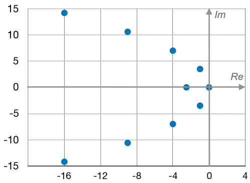
In particular, it can be checked that fη(0)=1subscript𝑓𝜂01f_{\eta}(0)=1 for all η0𝜂0\eta\neq 0, which means that there is a pole at the origin. Therefore, as in the inviscid case, the open loop system (20) is not asymptotically stable whatever the value of the viscosity η𝜂\eta. As a matter of illustration, in Figure 2, we present the spectrum of the system for η=0.1𝜂0.1\eta=0.1.

Refer to caption
Figure 2: The spectrum of the open loop system with viscosity η=0.1𝜂0.1\eta=0.1.

In the next section, we shall show that the system can be stabilized by output feedback when the (unknown) viscosity is small and even almost negligible.

4 Output feedback stabilization of the viscous system

We now assume that the open loop control system (20) is closed with a dead beat output feedback controller

U(t)=Y(t1).𝑈𝑡𝑌𝑡1U(t)=-Y(t-1). (32)

Note that this corresponds to the special case of the controller (10) where k1=0subscript𝑘10k_{1}=0, k2=1subscript𝑘21k_{2}=1 and τ=1/υ=1𝜏1𝜐1\tau=1/\upsilon=1. We know from Section 2 that, in this case, the inviscid system is exponentially stable but the stability is not robust to small perturbations in the propagation speeds. We shall show here that the exponential stability remains in the viscous system and we shall check in Section 5 that, in addition, the exponential stability is robust with small variations in the propagation speeds. In the frequency domain, the closed loop system (20), (32) is then:

y1(s,1)=fη(s)y1(s,0),subscripty1𝑠1subscript𝑓𝜂𝑠subscripty1𝑠0\displaystyle\textrm{y}_{\!1}(s,1)=f_{\eta}(s)\textrm{y}_{\!1}(s,0), (33a)
y2(s,1)=fη(s)y2(s,0),subscripty2𝑠1subscript𝑓𝜂𝑠subscripty2𝑠0\displaystyle\textrm{y}_{2}(s,1)=f_{\eta}(s)\textrm{y}_{2}(s,0), (33b)
y^2(s,1)=esy^2(s,0)subscript^y2𝑠1superscript𝑒𝑠subscript^y2𝑠0\displaystyle\hat{\textrm{y}}_{2}(s,1)=e^{-s}\hat{\textrm{y}}_{2}(s,0) (33c)
y1(s,0)=y2(s,1)y^2(s,1),subscripty1𝑠0subscripty2𝑠1subscript^y2𝑠1\displaystyle\textrm{y}_{\!1}(s,0)=\textrm{y}_{2}(s,1)-\hat{\textrm{y}}_{2}(s,1), (33d)
y2(s,0)=y1(s,1),subscripty2𝑠0subscripty1𝑠1\displaystyle\textrm{y}_{2}(s,0)=\textrm{y}_{\!1}(s,1), (33e)
y^2(s,0)=y1(s,1),subscript^y2𝑠0subscripty1𝑠1\displaystyle\hat{\textrm{y}}_{2}(s,0)=\textrm{y}_{\!1}(s,1), (33f)

From these equations, it follows that the characteristic equation of the closed loop system is:

fη2(s)fη(s)es1=0.superscriptsubscript𝑓𝜂2𝑠subscript𝑓𝜂𝑠superscript𝑒𝑠10f_{\eta}^{2}(s)-f_{\eta}(s)e^{-s}-1=0. (34)

Our purpose is now to address the stability of this closed loop system. For a given value of the viscosity η𝜂\eta, the spectrum 𝒮ηsubscript𝒮𝜂\mathcal{S}_{\eta} of the closed loop system is the set of the poles which are the roots of the characteristic equation (34):

𝒮η={s:fη2(s)fη(s)es1=0}.subscript𝒮𝜂conditional-set𝑠superscriptsubscript𝑓𝜂2𝑠subscript𝑓𝜂𝑠superscript𝑒𝑠10\mathcal{S}_{\eta}=\{s:f_{\eta}^{2}(s)-f_{\eta}(s)e^{-s}-1=0\}. (35)

Moreover, the maximal spectral abscissa is defined as the supremum of the real parts of the spectrum and denoted as follows:

ση=sup{Re(s):s𝒮η}.subscript𝜎𝜂supremumconditional-setRe𝑠𝑠subscript𝒮𝜂\sigma_{\eta}=\sup\{\text{Re}(s):s\in\mathcal{S}_{\eta}\}. (36)

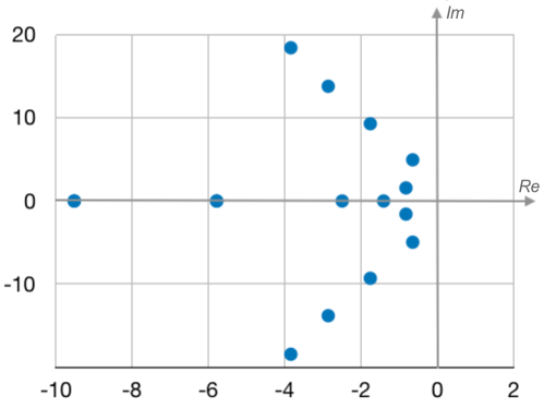
As a matter of illustration, we present in Figure 3 the spectrum of the closed loop system for η=0.1𝜂0.1\eta=0.1.

Refer to caption
Figure 3: The spectrum 𝒮ηsubscript𝒮𝜂\mathcal{S}_{\eta} of the closed loop system for η=0.1𝜂0.1\eta=0.1.

The stability of the closed loop system (33) can be deduced using the spectral mapping theorem. See [15, Chapter 9, Theorem 3.5] and [19] in the case η=0𝜂0\eta=0, and reference [6] for the case η0𝜂0\eta\neq 0. In particular the system is exponentially stable if (and only if) ση<0subscript𝜎𝜂0\sigma_{\eta}<0.

Then, one of the main results of this paper is given in the following stability theorem.

Theorem 1.

For any δ>0𝛿0\delta>0, there exists η1>0subscript𝜂10\eta_{1}>0 such that, for all η(0,η1)𝜂0subscript𝜂1\eta\in(0,\eta_{1}), the maximal spectral abscissa satisfies

σηln(2)+δ.subscript𝜎𝜂2𝛿\sigma_{\eta}\leqslant-\ln(2)+\delta. (37)

Conjecture 1.

The bound ln(2)2\ln(2) on the decay rate is optimal. More precisely, for any δ>0𝛿0\delta>0 and η1>0subscript𝜂10\eta_{1}>0 there exists η(0,η1)𝜂0subscript𝜂1\eta\in(0,\eta_{1}) such that the maximal abscissa satisfies

ln(2)δσηln(2)+δ.2𝛿subscript𝜎𝜂2𝛿-\ln(2)-\delta\leqslant\sigma_{\eta}\leqslant-\ln(2)+\delta. (38)

Remark 1 (Loss of continuity of the spectral abscissa).

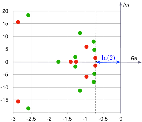
Conjecture 1 seems to be verified when looking at the spectrum numerically (see Figure 4). This would imply a loss of continuity in the sense that any decay rate is achievable when η=0𝜂0\eta=0. However there is a bound ln(2)2\ln(2) as soon as η>0𝜂0\eta>0, even if η𝜂\eta is arbitrarily small.

In order to prove Theorem 1, it is useful to define the complex variable

z=1+4ηs,𝑧14𝜂𝑠z=\sqrt{1+4\eta s}, (39)

where we recall that \sqrt{\cdot} is the principal value of the square root. The functions λ1subscript𝜆1\lambda_{1} and λ2subscript𝜆2\lambda_{2} become

λ1=(1+z)2ηandλ2=(1z)2η.formulae-sequencesubscript𝜆11𝑧2𝜂andsubscript𝜆21𝑧2𝜂\lambda_{1}=\dfrac{(1+z)}{2\eta}\hskip 14.22636pt\text{and}\hskip 14.22636pt\lambda_{2}=\dfrac{(1-z)}{2\eta}. (40)

Then, defining the function

Xη(z)=1+z2e(1z)/2η1z2e(1+z)/2η,subscript𝑋𝜂𝑧1𝑧2superscript𝑒1𝑧2𝜂1𝑧2superscript𝑒1𝑧2𝜂X_{\eta}(z)=\dfrac{1+z}{2}e^{-(1-z)/2\eta}-\dfrac{1-z}{2}e^{-(1+z)/2\eta}, (41)

we get, using (28), that the characteristic equation (34) is equivalent to

Xη2(z)+ze(z21)/4ηXη(z)z2=0.subscriptsuperscript𝑋2𝜂𝑧𝑧superscript𝑒superscript𝑧214𝜂subscript𝑋𝜂𝑧superscript𝑧20X^{2}_{\eta}(z)+ze^{-(z^{2}-1)/4\eta}X_{\eta}(z)-z^{2}=0. (42)

Let us now observe that Xη(0)=0subscript𝑋𝜂00X_{\eta}(0)=0. Consequently z=0𝑧0z=0 is a root of equation (42) for all η𝜂\eta. This implies obviously that s=1/4η𝒮η𝑠14𝜂subscript𝒮𝜂s=-1/4\eta\in\mathcal{S}_{\eta} is a pole of the system (i.e. a root of the characteristic equation (34)). Note that this pole tends to -\infty as η0+𝜂superscript0\eta\rightarrow 0^{+} so this is a very stable pole for small (positive) η𝜂\eta.

Let 𝒵ηsubscript𝒵𝜂\mathcal{Z}_{\eta} denote the set of non-zero roots of equation (42). Then, using definition (41) and solving equation (42) with respect to Xηsubscript𝑋𝜂X_{\eta}, we have that every z𝒵η𝑧subscript𝒵𝜂z\in\mathcal{Z}_{\eta} satisfies the equation

(1+z)ze(1z)/2η(1z)ze(1+z)/2η=e(z21)/4η±e(z21)/2η+4.1𝑧𝑧superscript𝑒1𝑧2𝜂1𝑧𝑧superscript𝑒1𝑧2𝜂plus-or-minussuperscript𝑒superscript𝑧214𝜂superscript𝑒superscript𝑧212𝜂4\dfrac{(1+z)}{z}e^{-(1-z)/2\eta}-\dfrac{(1-z)}{z}e^{-(1+z)/2\eta}=-e^{-(z^{2}-1)/4\eta}\pm\sqrt{e^{-(z^{2}-1)/2\eta}+4}. (43)

We now consider a sequence

(ηn)nwith0<ηn,nandlimn+ηn=0+,formulae-sequencesubscriptsubscript𝜂𝑛𝑛with0subscript𝜂𝑛formulae-sequencefor-all𝑛andsubscript𝑛subscript𝜂𝑛superscript0(\eta_{n})_{n\in\mathbb{N}}\hskip 14.22636pt\text{with}\hskip 14.22636pt0<\eta_{n}\in\mathbb{R},\;\forall n\in\mathbb{N}\hskip 14.22636pt\text{and}\hskip 14.22636pt\lim_{n\rightarrow+\infty}\eta_{n}=0^{+}, (44)

and an associated sequence

(sn)nsuch thatsn𝒮ηn,n.formulae-sequencesubscriptsubscript𝑠𝑛𝑛such thatsubscript𝑠𝑛subscript𝒮subscript𝜂𝑛for-all𝑛(s_{n})_{n\in\mathbb{N}}\hskip 14.22636pt\text{such that}\hskip 14.22636pts_{n}\in\mathcal{S}_{\eta_{n}},\forall n\in\mathbb{N}. (45)

In order to prove Theorem 1, we will look to the adherent points of the sequences (sn)nsubscriptsubscript𝑠𝑛𝑛(s_{n})_{n\in\mathbb{N}} when n+𝑛n\rightarrow+\infty (i.e. when ηn0+subscript𝜂𝑛superscript0\eta_{n}\rightarrow 0^{+}). By definition, we know that s¯¯𝑠\bar{s} is an adherent point of a sequence (sn)nsubscriptsubscript𝑠𝑛𝑛(s_{n})_{n\in\mathbb{N}} if and only if there exists a subsequence which converges to s¯¯𝑠\bar{s}. With a slight abuse of notation, we will write

sns¯orlimn+sn=s¯formulae-sequencesubscript𝑠𝑛¯𝑠orsubscript𝑛subscript𝑠𝑛¯𝑠s_{n}\longrightarrow\bar{s}\hskip 14.22636pt\text{or}\hskip 14.22636pt\lim_{n\rightarrow+\infty}s_{n}=\bar{s} (46)

to signify that s¯¯𝑠\bar{s} is an adherent point of a sequence (sn)nsubscriptsubscript𝑠𝑛𝑛(s_{n})_{n\in\mathbb{N}} but it is implied that the convergence in fact only relies on the adequate subsequence. This holds also for all other sequences that are introduced later in this article.

The proof of Theorem 1 is built from the two following lemmas.

Lemma 1.

Let (ηn)nsubscriptsubscript𝜂𝑛𝑛(\eta_{n})_{n\in\mathbb{N}} be a sequence of the form (44) and (zn)nsubscriptsubscript𝑧𝑛𝑛(z_{n})_{n\in\mathbb{N}} be any associated sequence of elements of 𝒵ηsubscript𝒵𝜂\mathcal{Z}_{\eta}. Let z¯¯𝑧\bar{z} be an adherent point of the sequence (zn)nsubscriptsubscript𝑧𝑛𝑛(z_{n})_{n\in\mathbb{N}}. Then

a)Re(z¯2)1(precisely: Re(z¯2)[,1]);a)Resuperscript¯𝑧21precisely: Resuperscript¯𝑧21\displaystyle\text{a)}\;\;\text{Re}(\bar{z}^{2})\leqslant 1\hskip 14.22636pt\big{(}\text{precisely: }\text{Re}(\bar{z}^{2})\in[-\infty,1]\;\big{)}; (47)
b)if Re(z¯2)=1 then (Re(z¯))2=1 and Im(z¯)=0.b)if Resuperscript¯𝑧21 then superscriptRe¯𝑧21 and Im¯𝑧0\displaystyle\text{b)}\;\;\text{if }\text{Re}(\bar{z}^{2})=1\text{ then }\left(\text{Re}(\bar{z})\right)^{\!2}=1\text{ and }\text{Im}(\bar{z})=0. (48)
Proof.

The proof of this lemma is given in Appendix B. ∎

Lemma 2.

Let (ηn)nsubscriptsubscript𝜂𝑛𝑛(\eta_{n})_{n\in\mathbb{N}} be a sequence of the form (44) and (sn)nsubscriptsubscript𝑠𝑛𝑛(s_{n})_{n\in\mathbb{N}} be any associated sequence of the form (45). Let s¯¯𝑠\bar{s} be an adherent point of (sn)nsubscriptsubscript𝑠𝑛𝑛(s_{n})_{n\in\mathbb{N}}. Then

Re(s¯)ln(2)(precisely: Re(s¯)[,ln(2)]).Re¯𝑠2precisely: Re¯𝑠2\text{Re}(\bar{s})\leqslant-\ln(2)\hskip 14.22636pt\big{(}\text{precisely: }\text{Re}(\bar{s})\in[-\infty,-\ln(2)]\;\big{)}. (49)
Proof.

Let s¯¯𝑠\bar{s} be an adherence point of the considered sequence (sn)nsubscriptsubscript𝑠𝑛𝑛(s_{n})_{n\in\mathbb{N}}. We restrict to a subsequence (still denoted (sn)nsubscriptsubscript𝑠𝑛𝑛(s_{n})_{n\in\mathbb{N}}) such that (sn)nsubscriptsubscript𝑠𝑛𝑛(s_{n})_{n\in\mathbb{N}} converges to s¯¯𝑠\bar{s}. Consider the sequence

(zn)nsuch thatzn=1+4ηsn,n.formulae-sequencesubscriptsubscript𝑧𝑛𝑛such thatsubscript𝑧𝑛14𝜂subscript𝑠𝑛for-all𝑛(z_{n})_{n\in\mathbb{N}}\hskip 14.22636pt\text{such that}\hskip 14.22636ptz_{n}=\sqrt{1+4\eta s_{n}},\forall n\in\mathbb{N}. (50)

By definition zn𝒵ηsubscript𝑧𝑛subscript𝒵𝜂z_{n}\in\mathcal{Z}_{\eta} for any n𝑛n\in\mathbb{N}. Let z¯¯𝑧\bar{z} be an adherence value of this sequence (zn)nsubscriptsubscript𝑧𝑛𝑛(z_{n})_{n\in\mathbb{N}} and let us again restrict to a subsequence (still denoted (zn)nsubscriptsubscript𝑧𝑛𝑛(z_{n})_{n\in\mathbb{N}}) that converges to z¯¯𝑧\bar{z}. Note that since it is a subsequence, we still have sns¯subscript𝑠𝑛¯𝑠s_{n}\rightarrow\bar{s}. From Lemma 1, we know that necessarily Re(z¯2)[,1]Resuperscript¯𝑧21\text{Re}(\bar{z}^{2})\in[-\infty,1].

Let us first assume that Re(z¯2)Resuperscript¯𝑧2\text{Re}(\bar{z}^{2}) is strictly smaller than 1, i.e. Re(z¯2)[,1)Resuperscript¯𝑧21\text{Re}(\bar{z}^{2})\in[-\infty,1). In that case, from the definition of snsubscript𝑠𝑛s_{n} in (45), we have

Re(s¯)=limn+Re(sn)=limn+Re(zn2)14ηn=limn+Re(zn2)1limn+4ηn=Re(z¯2)1limn+4ηn.Re¯𝑠subscript𝑛Resubscript𝑠𝑛subscript𝑛Resuperscriptsubscript𝑧𝑛214subscript𝜂𝑛subscript𝑛Resuperscriptsubscript𝑧𝑛21subscript𝑛4subscript𝜂𝑛Resuperscript¯𝑧21subscript𝑛4subscript𝜂𝑛\text{Re}(\bar{s})=\lim_{n\rightarrow+\infty}\text{Re}(s_{n})=\lim_{n\rightarrow+\infty}\dfrac{\text{Re}(z_{n}^{2})-1}{4\eta_{n}}=\dfrac{\lim_{n\rightarrow+\infty}\text{Re}(z_{n}^{2})-1}{\lim_{n\rightarrow+\infty}4\eta_{n}}=\dfrac{\text{Re}(\bar{z}^{2})-1}{\lim_{n\rightarrow+\infty}4\eta_{n}}. (51)

Since, by the definition (44), we know that limn+4ηn=0+subscript𝑛4subscript𝜂𝑛superscript0\lim_{n\rightarrow+\infty}4\eta_{n}=0^{+}, we can conclude

Re(s¯)=Re¯𝑠\text{Re}(\bar{s})=-\infty (52)

and the lemma is proved.

Let us now assume that Re(z¯2)=1Resuperscript¯𝑧21\text{Re}(\bar{z}^{2})=1. From Lemma 1 we know that, if Re(z¯2)=1Resuperscript¯𝑧21\text{Re}(\bar{z}^{2})=1, then necessarily Re(z¯)=±1Re¯𝑧plus-or-minus1\text{Re}(\bar{z})=\pm 1 and Im(z¯)=0Im¯𝑧0\text{Im}(\bar{z})=0; hence z¯=±1¯𝑧plus-or-minus1\bar{z}=\pm 1. We address the case where z¯=1¯𝑧1\bar{z}=1 (the reader can easily handle the case z¯=1¯𝑧1\bar{z}=-1 by symmetry) and we introduce the notations

yn=zn1,an=Re(yn),bn=Im(yn).formulae-sequencesubscript𝑦𝑛subscript𝑧𝑛1formulae-sequencesubscript𝑎𝑛Resubscript𝑦𝑛subscript𝑏𝑛Imsubscript𝑦𝑛y_{n}=z_{n}-1,\hskip 14.22636pta_{n}=\text{Re}(y_{n}),\hskip 14.22636ptb_{n}=\text{Im}(y_{n}). (53)

With these notations we have

Re(sn)=Re(zn2)14ηn=Re((yn+1)2)14ηn=an2bn24ηn+an2ηn.Resubscript𝑠𝑛Resuperscriptsubscript𝑧𝑛214subscript𝜂𝑛Resuperscriptsubscript𝑦𝑛1214subscript𝜂𝑛subscriptsuperscript𝑎2𝑛superscriptsubscript𝑏𝑛24subscript𝜂𝑛subscript𝑎𝑛2subscript𝜂𝑛\text{Re}(s_{n})=\dfrac{\text{Re}(z_{n}^{2})-1}{4\eta_{n}}=\dfrac{\text{Re}((y_{n}+1)^{2})-1}{4\eta_{n}}=\dfrac{a^{2}_{n}-b_{n}^{2}}{4\eta_{n}}+\dfrac{a_{n}}{2\eta_{n}}. (54)

Here the determination of adherent points of the sequence (Re(sn))nsubscriptResubscript𝑠𝑛𝑛(\text{Re}(s_{n}))_{n\in\mathbb{N}}, induced by the limit Re(zn)1Resubscript𝑧𝑛1\text{Re}(z_{n})\rightarrow 1 is clearly more delicate because it cannot be directly derived from formula (54) and requires a development which is detailed hereafter.

With the notation (53), the function Xηsubscript𝑋𝜂X_{\eta} defined in (41) becomes

Xη=(1+yn2)eyn/2ηn+yn2e1/ηnyn/2ηn,subscript𝑋𝜂1subscript𝑦𝑛2superscript𝑒subscript𝑦𝑛2subscript𝜂𝑛subscript𝑦𝑛2superscript𝑒1subscript𝜂𝑛subscript𝑦𝑛2subscript𝜂𝑛X_{\eta}=(1+\frac{y_{n}}{2})e^{y_{n}/2\eta_{n}}+\frac{y_{n}}{2}e^{-1/\eta_{n}-y_{n}/2\eta_{n}}, (55)

such that the characteristic equation (42) is written

((1+yn2)eyn/2ηn+yn2e1/ηnyn/2ηn)2superscript1subscript𝑦𝑛2superscript𝑒subscript𝑦𝑛2subscript𝜂𝑛subscript𝑦𝑛2superscript𝑒1subscript𝜂𝑛subscript𝑦𝑛2subscript𝜂𝑛2\displaystyle((1+\frac{y_{n}}{2})e^{y_{n}/2\eta_{n}}+\frac{y_{n}}{2}e^{-1/\eta_{n}-y_{n}/2\eta_{n}})^{2}
+(1+yn)eyn/2ηnyn2/4ηn[(1+yn2)eyn/2ηn+yn2e1/4ηnyn/2ηn]=(1+yn)2.1subscript𝑦𝑛superscript𝑒subscript𝑦𝑛2subscript𝜂𝑛superscriptsubscript𝑦𝑛24subscript𝜂𝑛delimited-[]1subscript𝑦𝑛2superscript𝑒subscript𝑦𝑛2subscript𝜂𝑛subscript𝑦𝑛2superscript𝑒14subscript𝜂𝑛subscript𝑦𝑛2subscript𝜂𝑛superscript1subscript𝑦𝑛2\displaystyle\hskip 28.45274pt\hskip 28.45274pt+(1+y_{n})e^{-y_{n}/2\eta_{n}-y_{n}^{2}/4\eta_{n}}[(1+\frac{y_{n}}{2})e^{y_{n}/2\eta_{n}}+\frac{y_{n}}{2}e^{-1/4\eta_{n}-y_{n}/2\eta_{n}}]=(1+y_{n})^{2}. (56)

Now, because ηn0+subscript𝜂𝑛superscript0\eta_{n}\rightarrow 0^{+} and yn0subscript𝑦𝑛0y_{n}\rightarrow 0 (since znz¯subscript𝑧𝑛¯𝑧z_{n}\rightarrow\bar{z}), we have

(1+yn2)2eyn/ηn+o(e1/ηn)superscript1subscript𝑦𝑛22superscript𝑒subscript𝑦𝑛subscript𝜂𝑛𝑜superscript𝑒1subscript𝜂𝑛\displaystyle(1+\frac{y_{n}}{2})^{2}e^{y_{n}/\eta_{n}}+o(e^{-1/\eta_{n}})
+(1+yn)(1+yn2)eyn2/4ηn+o(e1/4ηnyn/ηnyn2/4ηn)=(1+yn)2.1subscript𝑦𝑛1subscript𝑦𝑛2superscript𝑒superscriptsubscript𝑦𝑛24subscript𝜂𝑛𝑜superscript𝑒14subscript𝜂𝑛subscript𝑦𝑛subscript𝜂𝑛superscriptsubscript𝑦𝑛24subscript𝜂𝑛superscript1subscript𝑦𝑛2\displaystyle\hskip 28.45274pt\hskip 28.45274pt+(1+y_{n})(1+\frac{y_{n}}{2})e^{-y_{n}^{2}/4\eta_{n}}+o(e^{-1/4\eta_{n}-y_{n}/\eta_{n}-y_{n}^{2}/4\eta_{n}})=(1+y_{n})^{2}. (57)

This implies that, for n+𝑛n\rightarrow+\infty,

eyn/ηn+1+yn1+yn2eyn2/4ηn1.superscript𝑒subscript𝑦𝑛subscript𝜂𝑛1subscript𝑦𝑛1subscript𝑦𝑛2superscript𝑒superscriptsubscript𝑦𝑛24subscript𝜂𝑛1e^{y_{n}/\eta_{n}}+\frac{1+y_{n}}{1+\frac{y_{n}}{2}}e^{-y_{n}^{2}/4\eta_{n}}\longrightarrow 1. (58)

With (54), (58) becomes

ean/ηneibn/ηn+(1+an+ibn)(1+an/2ibn/2)|1+yn2|2ean2/4ηnebn2/4ηneianbn/2ηn1,superscript𝑒subscript𝑎𝑛subscript𝜂𝑛superscript𝑒𝑖subscript𝑏𝑛subscript𝜂𝑛1subscript𝑎𝑛𝑖subscript𝑏𝑛1subscript𝑎𝑛2𝑖subscript𝑏𝑛2superscript1subscript𝑦𝑛22superscript𝑒superscriptsubscript𝑎𝑛24subscript𝜂𝑛superscript𝑒superscriptsubscript𝑏𝑛24subscript𝜂𝑛superscript𝑒𝑖subscript𝑎𝑛subscript𝑏𝑛2subscript𝜂𝑛1e^{a_{n}/\eta_{n}}e^{ib_{n}/\eta_{n}}+\frac{(1+a_{n}+ib_{n})(1+a_{n}/2-ib_{n}/2)}{|1+\frac{y_{n}}{2}|^{2}}e^{-a_{n}^{2}/4\eta_{n}}e^{b_{n}^{2}/4\eta_{n}}e^{-ia_{n}b_{n}/2\eta_{n}}\rightarrow 1, (59)

or, separating the real and imaginary parts,

ean/ηncos(bnηn)+ean2/4ηnebn2/4ηn[(1+3an+an2+bn22)cos(anbn2ηn)+bn2sin(anbn2ηn)]1|1+yn2|21,superscript𝑒subscript𝑎𝑛subscript𝜂𝑛subscript𝑏𝑛subscript𝜂𝑛superscript𝑒superscriptsubscript𝑎𝑛24subscript𝜂𝑛superscript𝑒superscriptsubscript𝑏𝑛24subscript𝜂𝑛delimited-[]13subscript𝑎𝑛superscriptsubscript𝑎𝑛2superscriptsubscript𝑏𝑛22subscript𝑎𝑛subscript𝑏𝑛2subscript𝜂𝑛subscript𝑏𝑛2subscript𝑎𝑛subscript𝑏𝑛2subscript𝜂𝑛1superscript1subscript𝑦𝑛221\displaystyle e^{a_{n}/\eta_{n}}\cos({\textstyle\frac{b_{n}}{\eta_{n}}})+e^{-a_{n}^{2}/4\eta_{n}}e^{b_{n}^{2}/4\eta_{n}}\left[\left(1+{\textstyle\frac{3a_{n}+a_{n}^{2}+b_{n}^{2}}{2}}\right)\cos({\textstyle\frac{a_{n}b_{n}}{2\eta_{n}}})+{\textstyle\frac{b_{n}}{2}}\sin({\textstyle\frac{a_{n}b_{n}}{2\eta_{n}}})\right]\frac{1}{|1+\frac{y_{n}}{2}|^{2}}\rightarrow 1, (60)
ean/ηnsin(bnηn)+ean2/4ηnebn2/4ηn[(1+3an+an2+bn22)sin(anbn2ηn)+bn2cos(anbn2ηn)]1|1+yn2|20.superscript𝑒subscript𝑎𝑛subscript𝜂𝑛subscript𝑏𝑛subscript𝜂𝑛superscript𝑒superscriptsubscript𝑎𝑛24subscript𝜂𝑛superscript𝑒superscriptsubscript𝑏𝑛24subscript𝜂𝑛delimited-[]13subscript𝑎𝑛superscriptsubscript𝑎𝑛2superscriptsubscript𝑏𝑛22subscript𝑎𝑛subscript𝑏𝑛2subscript𝜂𝑛subscript𝑏𝑛2subscript𝑎𝑛subscript𝑏𝑛2subscript𝜂𝑛1superscript1subscript𝑦𝑛220\displaystyle e^{a_{n}/\eta_{n}}\sin({\textstyle\frac{b_{n}}{\eta_{n}}})+e^{-a_{n}^{2}/4\eta_{n}}e^{b_{n}^{2}/4\eta_{n}}\left[-\left(1+{\textstyle\frac{3a_{n}+a_{n}^{2}+b_{n}^{2}}{2}}\right)\sin({\textstyle\frac{a_{n}b_{n}}{2\eta_{n}}})+{\textstyle\frac{b_{n}}{2}}\cos({\textstyle\frac{a_{n}b_{n}}{2\eta_{n}}})\right]\frac{1}{|1+\frac{y_{n}}{2}|^{2}}\rightarrow 0. (61)

Let us now denote a¯¯𝑎\bar{a} an adherence point of the sequence (an/2ηn)nsubscriptsubscript𝑎𝑛2subscript𝜂𝑛𝑛(a_{n}/2\eta_{n})_{n\in\mathbb{N}}. We shall discuss successively the three cases : a¯=¯𝑎\bar{a}=-\infty, a¯(,+)¯𝑎\bar{a}\in(-\infty,+\infty) and a¯=+¯𝑎\bar{a}=+\infty.

The case 𝐚¯=.¯𝐚\mathbf{\bar{a}=-\infty.}
In this case the lemma is trivial because, since an0subscript𝑎𝑛0a_{n}\rightarrow 0 and an/2ηna¯=subscript𝑎𝑛2subscript𝜂𝑛¯𝑎a_{n}/2\eta_{n}\rightarrow\bar{a}=-\infty, then an2/4ηn+an/2ηnsuperscriptsubscript𝑎𝑛24subscript𝜂𝑛subscript𝑎𝑛2subscript𝜂𝑛a_{n}^{2}/4\eta_{n}+a_{n}/2\eta_{n}\rightarrow-\infty and therefore, from (54), Re(s¯)=Re¯𝑠\text{Re}(\bar{s})=-\infty.

The case 𝐚¯(,+).¯𝐚\mathbf{\bar{a}\in(-\infty,+\infty).}

In this case an2/2ηn0superscriptsubscript𝑎𝑛22subscript𝜂𝑛0a_{n}^{2}/2\eta_{n}\rightarrow 0 and anbn/2ηn0subscript𝑎𝑛subscript𝑏𝑛2subscript𝜂𝑛0a_{n}b_{n}/2\eta_{n}\rightarrow 0 because an+ibn=yn0subscript𝑎𝑛𝑖subscript𝑏𝑛subscript𝑦𝑛0a_{n}+ib_{n}=y_{n}\rightarrow 0 while an/2ηna¯subscript𝑎𝑛2subscript𝜂𝑛¯𝑎a_{n}/2\eta_{n}\rightarrow\bar{a}\in\mathbb{R}. Then from (60), we have

ean/ηncos(bnηn)+ebn2/4ηn(1+o(1))1.superscript𝑒subscript𝑎𝑛subscript𝜂𝑛subscript𝑏𝑛subscript𝜂𝑛superscript𝑒superscriptsubscript𝑏𝑛24subscript𝜂𝑛1𝑜11e^{a_{n}/\eta_{n}}\cos({\textstyle\frac{b_{n}}{\eta_{n}}})+e^{b_{n}^{2}/4\eta_{n}}(1+o(1))\longrightarrow 1. (62)

Let us now denote c¯[0,+]¯𝑐0\bar{c}\in[0,+\infty] an adherence point of the sequence (bn2/4ηn)nsubscriptsuperscriptsubscript𝑏𝑛24subscript𝜂𝑛𝑛(b_{n}^{2}/4\eta_{n})_{n\in\mathbb{N}} and κ¯[1,1]¯𝜅11\bar{\kappa}\in[-1,1] an adherent point of the sequence (cos(bnηn))nsubscriptsubscript𝑏𝑛subscript𝜂𝑛𝑛(\cos({\textstyle\frac{b_{n}}{\eta_{n}}}))_{n\in\mathbb{N}}. Then, taking the limit111This can be done by restricting to a subsequence where both (bn2/4ηn)nsubscriptsuperscriptsubscript𝑏𝑛24subscript𝜂𝑛𝑛(b_{n}^{2}/4\eta_{n})_{n\in\mathbb{N}} and (cos(bnηn))nsubscriptsubscript𝑏𝑛subscript𝜂𝑛𝑛(\cos({\textstyle\frac{b_{n}}{\eta_{n}}}))_{n\in\mathbb{N}} converge, using a diagonal argument., we have from (62)

e2a¯κ¯+ec¯=1.superscript𝑒2¯𝑎¯𝜅superscript𝑒¯𝑐1e^{2\bar{a}}\bar{\kappa}+e^{\bar{c}}=1. (63)

Because ea¯superscript𝑒¯𝑎e^{\bar{a}} is bounded and ea¯>0superscript𝑒¯𝑎0e^{\bar{a}}>0, and bn2/4ηn0superscriptsubscript𝑏𝑛24subscript𝜂𝑛0b_{n}^{2}/4\eta_{n}\geq 0 for any n𝑛n\in\mathbb{N}, this implies necessarily that

c¯[0,+)andec¯1andκ¯[1,0].formulae-sequence¯𝑐0andformulae-sequencesuperscript𝑒¯𝑐1and¯𝜅10\bar{c}\in[0,+\infty)\hskip 14.22636pt\text{and}\hskip 14.22636pte^{\bar{c}}\geqslant 1\hskip 14.22636pt\text{and}\hskip 14.22636pt\bar{\kappa}\in[-1,0]. (64)

Then it means in particular that bn2/ηnsuperscriptsubscript𝑏𝑛2subscript𝜂𝑛b_{n}^{2}/\eta_{n} is bounded when ηn0+subscript𝜂𝑛superscript0\eta_{n}\rightarrow 0^{+}, and from (61) we deduce that

ean/ηnsin(bnηn)+o(1)0superscript𝑒subscript𝑎𝑛subscript𝜂𝑛subscript𝑏𝑛subscript𝜂𝑛𝑜10e^{a_{n}/\eta_{n}}\sin({\textstyle\frac{b_{n}}{\eta_{n}}})+o(1)\longrightarrow 0 (65)

which implies that sin(bnηn)0subscript𝑏𝑛subscript𝜂𝑛0\sin({\textstyle\frac{b_{n}}{\eta_{n}}})\rightarrow 0 and therefore that the only possible adherence points for cos(bnηn)subscript𝑏𝑛subscript𝜂𝑛\cos({\textstyle\frac{b_{n}}{\eta_{n}}}) are κ¯=±1¯𝜅plus-or-minus1\bar{\kappa}=\pm 1. Since κ¯[1,0]¯𝜅10\bar{\kappa}\in[-1,0], we deduce that κ¯=1¯𝜅1\bar{\kappa}=-1. Therefore, from (63),

ec¯=1+e2a¯.superscript𝑒¯𝑐1superscript𝑒2¯𝑎e^{\bar{c}}=1+e^{2\bar{a}}. (66)

Let us now consider the function eRe(sn)superscript𝑒Resubscript𝑠𝑛e^{-\text{Re}(s_{n})} with Re(sn)Resubscript𝑠𝑛\text{Re}(s_{n}) given by (54):

eRe(sn)=e(bn2an2)/4ηnan/2ηnec¯ea¯=ea¯+ea¯=2cosh(a¯)2.superscript𝑒Resubscript𝑠𝑛superscript𝑒superscriptsubscript𝑏𝑛2superscriptsubscript𝑎𝑛24subscript𝜂𝑛subscript𝑎𝑛2subscript𝜂𝑛superscript𝑒¯𝑐superscript𝑒¯𝑎superscript𝑒¯𝑎superscript𝑒¯𝑎2¯𝑎2e^{-\text{Re}(s_{n})}=e^{(b_{n}^{2}-a_{n}^{2})/4\eta_{n}-a_{n}/2\eta_{n}}\longrightarrow e^{\bar{c}}e^{-\bar{a}}=e^{-\bar{a}}+e^{\bar{a}}=2\cosh(\bar{a})\geqslant 2. (67)

It follows directly that

Re(s¯)ln(2)Re¯𝑠2\text{Re}(\bar{s})\leqslant-\ln(2) (68)

and the lemma is proved.

The case 𝐚¯=+.¯𝐚\mathbf{\bar{a}=+\infty.}

In this case we first observe that e(an2bn2)/4ηnan/2ηn0superscript𝑒superscriptsubscript𝑎𝑛2superscriptsubscript𝑏𝑛24subscript𝜂𝑛subscript𝑎𝑛2subscript𝜂𝑛0e^{(a_{n}^{2}-b_{n}^{2})/4\eta_{n}-a_{n}/2\eta_{n}}\rightarrow 0. Then multiplying both sides of (60) by this quantity, we get:

e(an2bn2)/4ηn+an/2ηncos(bnηn)+ean/2ηn[(1+3an+an2+bn22)cos(anbn2ηn)+bn2sin(anbn2ηn)]1|1+yn2|2superscript𝑒superscriptsubscript𝑎𝑛2superscriptsubscript𝑏𝑛24subscript𝜂𝑛subscript𝑎𝑛2subscript𝜂𝑛subscript𝑏𝑛subscript𝜂𝑛superscript𝑒subscript𝑎𝑛2subscript𝜂𝑛delimited-[]13subscript𝑎𝑛superscriptsubscript𝑎𝑛2superscriptsubscript𝑏𝑛22subscript𝑎𝑛subscript𝑏𝑛2subscript𝜂𝑛subscript𝑏𝑛2subscript𝑎𝑛subscript𝑏𝑛2subscript𝜂𝑛1superscript1subscript𝑦𝑛22\displaystyle e^{(a_{n}^{2}-b_{n}^{2})/4\eta_{n}+a_{n}/2\eta_{n}}\cos({\textstyle\frac{b_{n}}{\eta_{n}}})+e^{-a_{n}/2\eta_{n}}\left[(1+{\textstyle\frac{3a_{n}+a_{n}^{2}+b_{n}^{2}}{2}})\cos({\textstyle\frac{a_{n}b_{n}}{2\eta_{n}}})+{\textstyle\frac{b_{n}}{2}}\sin({\textstyle\frac{a_{n}b_{n}}{2\eta_{n}}})\right]\frac{1}{|1+\frac{y_{n}}{2}|^{2}}
e(an2bn2)/4ηnan/2ηn0,superscript𝑒superscriptsubscript𝑎𝑛2superscriptsubscript𝑏𝑛24subscript𝜂𝑛subscript𝑎𝑛2subscript𝜂𝑛0\displaystyle\hskip 227.62204pt-e^{(a_{n}^{2}-b_{n}^{2})/4\eta_{n}-a_{n}/2\eta_{n}}\rightarrow 0, (69)

From this expression, we deduce that

e(an2bn2)/4ηn+an/2ηncos(bnηn)0.superscript𝑒superscriptsubscript𝑎𝑛2superscriptsubscript𝑏𝑛24subscript𝜂𝑛subscript𝑎𝑛2subscript𝜂𝑛subscript𝑏𝑛subscript𝜂𝑛0e^{(a_{n}^{2}-b_{n}^{2})/4\eta_{n}+a_{n}/2\eta_{n}}\cos({\textstyle\frac{b_{n}}{\eta_{n}}})\longrightarrow 0. (70)

A similar manipulation of (61) gives

e(an2bn2)/4ηn+an/2ηnsin(bnηn)0.superscript𝑒superscriptsubscript𝑎𝑛2superscriptsubscript𝑏𝑛24subscript𝜂𝑛subscript𝑎𝑛2subscript𝜂𝑛subscript𝑏𝑛subscript𝜂𝑛0e^{(a_{n}^{2}-b_{n}^{2})/4\eta_{n}+a_{n}/2\eta_{n}}\sin({\textstyle\frac{b_{n}}{\eta_{n}}})\longrightarrow 0. (71)

Combining (70) and (71) we obtain

e(an2bn2)/2ηn+an/ηn=e2Re(sn)0superscript𝑒superscriptsubscript𝑎𝑛2superscriptsubscript𝑏𝑛22subscript𝜂𝑛subscript𝑎𝑛subscript𝜂𝑛superscript𝑒2Resubscript𝑠𝑛0e^{(a_{n}^{2}-b_{n}^{2})/2\eta_{n}+a_{n}/\eta_{n}}=e^{2\text{Re}(s_{n})}\longrightarrow 0 (72)

which implies that Re(sn)Resubscript𝑠𝑛\text{Re}(s_{n})\rightarrow-\infty and the lemma is proved. ∎

Based on Lemma 2, we can now give the following proof of Theorem 1.

Proof of Theorem 1.
We assume by contradiction that the theorem does not hold:

For any δ>0,η1>0 such that σηln(2)+δη(0,η1).formulae-sequenceFor any 𝛿0not-existssubscript𝜂10 such that subscript𝜎𝜂2𝛿for-all𝜂0subscript𝜂1\text{For any }\delta>0,\nexists\,\eta_{1}>0\text{ such that }\sigma_{\eta}\leqslant-\ln(2)+\delta\;\;\forall\eta\in(0,\eta_{1}). (73)

This implies that

For all η>0,η1(0,η) and s𝒮η1 such that Re(s)>ln(2)+δ.formulae-sequenceFor all 𝜂0subscript𝜂10𝜂 and 𝑠subscript𝒮subscript𝜂1 such that Re𝑠2𝛿\text{For all }\eta>0,\;\exists\eta_{1}\in(0,\eta)\text{ and }\exists s\in\mathcal{S}_{\eta_{1}}\text{ such that }\text{Re}(s)>-\ln(2)+\delta. (74)

It follows that we can build a sequence (ηn)nsubscriptsubscript𝜂𝑛𝑛(\eta_{n})_{n\in\mathbb{N}} of the form (44) and an associated sequence (sn)nsubscriptsubscript𝑠𝑛𝑛(s_{n})_{n\in\mathbb{N}} with sn𝒮ηnsubscript𝑠𝑛subscript𝒮subscript𝜂𝑛s_{n}\in\mathcal{S}_{\eta_{n}}. For this sequence we deduce from (74) that necessarily Re(s¯)>ln(2)+δRe¯𝑠2𝛿\text{Re}(\bar{s})>-\ln(2)+\delta, which is in contradiction with Lemma 2. ∎
Refer to caption
Figure 4: The spectrum 𝒮ηsubscript𝒮𝜂\mathcal{S}_{\eta} of the closed loop system for η=0.02𝜂0.02\eta=0.02 and η=0.2𝜂0.2\eta=0.2 .

The theorem is illustrated in Figure 4 where the spectrum is represented for the values η𝜂\eta = 0.02 and 0.2, and where the effectiveness of the stability margin ln(2)2-\ln(2) can be appreciated.

5 Robustness analysis

We consider again the control problem of the previous section. However, because we want to explicitly account for the sensitivity to delay uncertainties, we introduce an additional perturbation ε𝜀\varepsilon to the nominal transport velocity υ=1𝜐1\upsilon=1. The open loop system is therefore written in the time domain as follows:

ty1(t,x)+(1+ε)xy1(t,x)ηxx2y1(t,x)=0,subscript𝑡subscript𝑦1𝑡𝑥1𝜀subscript𝑥subscript𝑦1𝑡𝑥𝜂subscriptsuperscript2𝑥𝑥subscript𝑦1𝑡𝑥0\displaystyle\partial_{t}y_{1}(t,x)+(1+\varepsilon)\partial_{x}y_{1}(t,x)-\eta\partial^{2}_{xx}y_{1}(t,x)=0, (75a)
ty2(t,x)+(1+ε)xy2(t,x)ηxx2y2(t,x)=0,subscript𝑡subscript𝑦2𝑡𝑥1𝜀subscript𝑥subscript𝑦2𝑡𝑥𝜂subscriptsuperscript2𝑥𝑥subscript𝑦2𝑡𝑥0\displaystyle\partial_{t}y_{2}(t,x)+(1+\varepsilon)\partial_{x}y_{2}(t,x)-\eta\partial^{2}_{xx}y_{2}(t,x)=0, (75b)
y1(t,0)=y2(t,1)+U(t),subscript𝑦1𝑡0subscript𝑦2𝑡1𝑈𝑡\displaystyle y_{1}(t,0)=y_{2}(t,1)+U(t), (75c)
y2(t,0)=y1(t,1),subscript𝑦2𝑡0subscript𝑦1𝑡1\displaystyle y_{2}(t,0)=y_{1}(t,1), (75d)
xy1(t,1)=xy2(t,1)=0subscript𝑥subscript𝑦1𝑡1subscript𝑥subscript𝑦2𝑡10\displaystyle\partial_{x}y_{1}(t,1)=\partial_{x}y_{2}(t,1)=0 (75e)
Y(t)=y1(t,1),𝑌𝑡subscript𝑦1𝑡1\displaystyle Y(t)=y_{1}(t,1), (75f)

We suppose, as before, that the system is closed with the dead beat output feedback controller

U(t)=Y(t1).𝑈𝑡𝑌𝑡1U(t)=-Y(t-1). (76)

Remark that this control law depends on the theoretical delay (τ=1𝜏1\tau=1), ignoring the uncertainty represented by ε𝜀\varepsilon.

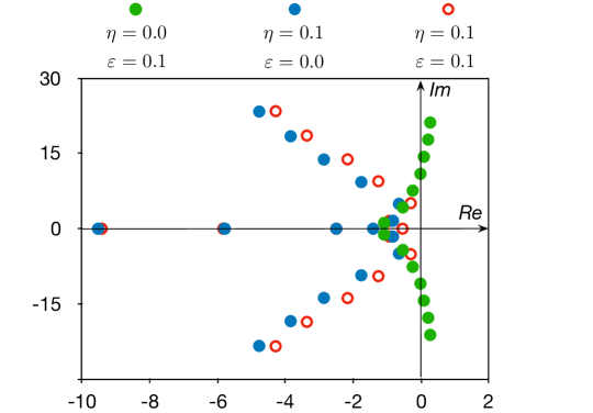
Remark also that for simplicity we assume here that we have the same uncertainty ε𝜀\varepsilon on both physical subsystems represented by transport equations (75a) and (75b). This may seem like a simplification but, actually, it can be shown that this single perturbation, even if it is arbitrarily small, is sufficient to destroy the closed loop stability when η=0𝜂0\eta=0 (see Figure 5 hereafter).

In this case the transfer functions of the two transport subsystems become

fη,ε(s)=λ1(s)λ2(s)λ1(s)eλ2(s)λ2(s)eλ1(s).subscript𝑓𝜂𝜀𝑠subscript𝜆1𝑠subscript𝜆2𝑠subscript𝜆1𝑠superscript𝑒subscript𝜆2𝑠subscript𝜆2𝑠superscript𝑒subscript𝜆1𝑠f_{\eta,\varepsilon}(s)=\dfrac{\lambda_{1}(s)-\lambda_{2}(s)}{\lambda_{1}(s)e^{-\lambda_{2}(s)}-\lambda_{2}(s)e^{-\lambda_{1}(s)}}. (77)

with the function fη,εsubscript𝑓𝜂𝜀f_{\eta,\varepsilon} now depending on both η𝜂\eta and ε𝜀\varepsilon because the functions λ1subscript𝜆1\lambda_{1} and λ2subscript𝜆2\lambda_{2} are modified as follows:

λ1(s)=(1+ε)+(1+ε)2+4ηs2η,λ2(s)=(1+ε)(1+ε)2+4ηs2η.formulae-sequencesubscript𝜆1𝑠1𝜀superscript1𝜀24𝜂𝑠2𝜂subscript𝜆2𝑠1𝜀superscript1𝜀24𝜂𝑠2𝜂\lambda_{1}(s)=\dfrac{(1+\varepsilon)+\sqrt{(1+\varepsilon)^{2}+4\eta s}}{2\eta},\hskip 14.22636pt\lambda_{2}(s)=\dfrac{(1+\varepsilon)-\sqrt{(1+\varepsilon)^{2}+4\eta s}}{2\eta}. (78)

With this definition, the characteristic equation of the closed loop system is now

fη,ε2(s)fη,ε(s)es1=0.superscriptsubscript𝑓𝜂𝜀2𝑠subscript𝑓𝜂𝜀𝑠superscript𝑒𝑠10f_{\eta,\varepsilon}^{2}(s)-f_{\eta,\varepsilon}(s)e^{-s}-1=0. (79)

As in the previous section, we introduce the spectrum 𝒮η,εsubscript𝒮𝜂𝜀\mathcal{S}_{\eta,\varepsilon} and the maximal abscissa ση,εsubscript𝜎𝜂𝜀\sigma_{\eta,\varepsilon} defined by

𝒮η,ε={s:s is solution of (79)},subscript𝒮𝜂𝜀conditional-set𝑠𝑠 is solution of italic-(79italic-)\displaystyle\mathcal{S}_{\eta,\varepsilon}=\{s\in\mathbb{C}:s\text{ is solution of }\eqref{charac4}\}, (80)
ση,ε=sup{Re(s):s𝒮η,ε}.subscript𝜎𝜂𝜀supremumconditional-setRe𝑠𝑠subscript𝒮𝜂𝜀\displaystyle\sigma_{\eta,\varepsilon}=\sup\{\text{Re}(s):s\in\mathcal{S}_{\eta,\varepsilon}\}. (81)

We remark that, by definition, we have

𝒮η,0=𝒮η and ση,0=ση.formulae-sequencesubscript𝒮𝜂0subscript𝒮𝜂 and subscript𝜎𝜂0subscript𝜎𝜂\mathcal{S}_{\eta,0}=\mathcal{S}_{\eta}\hskip 14.22636pt\text{ and }\hskip 14.22636pt\sigma_{\eta,0}=\sigma_{\eta}. (82)

We then have the following robustness theorem.

Theorem 2.

Let δ>0𝛿0\delta>0 and η>0𝜂0\eta>0 be such that Theorem 1 holds, i.e.

ση,0ln(2)+δ.subscript𝜎𝜂0ln2𝛿\sigma_{\eta,0}\leqslant-\text{ln}(2)+\delta. (83)

Then there exists ε1>0subscript𝜀10\varepsilon_{1}>0 such that for any ε(ε1,ε1)𝜀subscript𝜀1subscript𝜀1\varepsilon\in(-\varepsilon_{1},\varepsilon_{1}) the maximal spectral abscissa ση,εsubscript𝜎𝜂𝜀\sigma_{\eta,\varepsilon} satisfies

ση,εln(2)+2δsubscript𝜎𝜂𝜀ln22𝛿\sigma_{\eta,\varepsilon}\leqslant-\text{ln}(2)+2\delta (84)
Proof.

We proceed by contradiction and we assume that Theorem 2 does not hold. This implies that for any ε1>0subscript𝜀10\varepsilon_{1}>0 there exists ε(ε1,ε1)𝜀subscript𝜀1subscript𝜀1\varepsilon\in(-\varepsilon_{1},\varepsilon_{1}) such that

ση,ε>ln(2)+2δ,subscript𝜎𝜂𝜀ln22𝛿\sigma_{\eta,\varepsilon}>-\text{ln}(2)+2\delta, (85)

and therefore that there exists s𝒮η,ε𝑠subscript𝒮𝜂𝜀s\in\mathcal{S}_{\eta,\varepsilon} such that

Re(s)>ln(2)+2δ.Re𝑠ln22𝛿\text{Re}(s)>-\text{ln}(2)+2\delta. (86)

Hence we can define a sequence

(εn)nwithlimn+εn=0,subscriptsubscript𝜀𝑛𝑛withsubscript𝑛subscript𝜀𝑛0(\varepsilon_{n})_{n\in\mathbb{N}}\hskip 14.22636pt\text{with}\hskip 14.22636pt\lim_{n\rightarrow+\infty}\varepsilon_{n}=0, (87)

and an associated sequence (sn)nsubscriptsubscript𝑠𝑛𝑛(s_{n})_{n\in\mathbb{N}} such that

Re(sn)>ln(2)+2δ,withsn𝒮η,εnn.formulae-sequenceResubscript𝑠𝑛ln22𝛿withsubscript𝑠𝑛subscript𝒮𝜂subscript𝜀𝑛for-all𝑛\text{Re}(s_{n})>-\text{ln}(2)+2\delta,\;\;\text{with}\;\;s_{n}\in\mathcal{S}_{\eta,\varepsilon_{n}}\;\forall n\in\mathbb{N}. (88)
  • If the sequence (sn)nsubscriptsubscript𝑠𝑛𝑛(s_{n})_{n\in\mathbb{N}} is bounded, then we can extract a subsequence that converges to a limit s¯¯𝑠\bar{s}\in\mathbb{C}. We still denote this subsequence by (sn)nsubscriptsubscript𝑠𝑛𝑛(s_{n})_{n\in\mathbb{N}}. As εn0subscript𝜀𝑛0\varepsilon_{n}\rightarrow 0 we can pass to the limit in (79) and deduce that s¯𝒮η,0=𝒮η¯𝑠subscript𝒮𝜂0subscript𝒮𝜂\bar{s}\in\mathcal{S}_{\eta,0}=\mathcal{S}_{\eta} and therefore, from the assumption on δ𝛿\delta and η𝜂\eta, that

    Re(s¯)ln(2)+δ.Re¯𝑠ln2𝛿\text{Re}(\bar{s})\leqslant-\text{ln}(2)+\delta. (89)

    On the other hand, again passing to the limit, we deduce from (88) that

    Re(s¯)ln(2)+2δ>ln(2)+δ,Re¯𝑠ln22𝛿ln2𝛿\text{Re}(\bar{s})\geqslant-\text{ln}(2)+2\delta>-\text{ln}(2)+\delta, (90)

    which is in contradiction with (89).

  • If the sequence (sn)nsubscriptsubscript𝑠𝑛𝑛(s_{n})_{n\in\mathbb{N}} is unbounded, then we can extract a subsequence such that |sn|+subscript𝑠𝑛|s_{n}|\rightarrow+\infty. We still denote this subsequence by (sn)nsubscriptsubscript𝑠𝑛𝑛(s_{n})_{n\in\mathbb{N}}. We denote sn=rneiθnsubscript𝑠𝑛subscript𝑟𝑛superscript𝑒𝑖subscript𝜃𝑛s_{n}=r_{n}e^{i\theta_{n}}, with rn+subscript𝑟𝑛subscriptr_{n}\in\mathbb{R}_{+} and θn[π,π)subscript𝜃𝑛𝜋𝜋\theta_{n}\in[-\pi,\pi), for n𝑛n\in\mathbb{N}. Since rn=|sn|+subscript𝑟𝑛subscript𝑠𝑛r_{n}=|s_{n}|\rightarrow+\infty and (88) holds, we deduce that for n𝑛n sufficiently large θn(5π/8,5π/8)subscript𝜃𝑛5𝜋85𝜋8\theta_{n}\in(-5\pi/8,5\pi/8). Denoting (1+εn)+4ηsn=rn1eiθn11subscript𝜀𝑛4𝜂subscript𝑠𝑛superscriptsubscript𝑟𝑛1superscript𝑒𝑖superscriptsubscript𝜃𝑛1(1+\varepsilon_{n})+4\eta s_{n}=r_{n}^{1}e^{i\theta_{n}^{1}} with rn1+superscriptsubscript𝑟𝑛1subscriptr_{n}^{1}\in\mathbb{R}_{+} and θn1[π,π)subscriptsuperscript𝜃1𝑛𝜋𝜋\theta^{1}_{n}\in[-\pi,\pi) we deduce that for n𝑛n sufficiently large (depending on η𝜂\eta), rn1+superscriptsubscript𝑟𝑛1r_{n}^{1}\rightarrow+\infty and θn1(3π/4,3π/4)superscriptsubscript𝜃𝑛13𝜋43𝜋4\theta_{n}^{1}\in(-3\pi/4,3\pi/4). Thus

    (1+εn)+4ηsn=rn1eiθn1/2,1subscript𝜀𝑛4𝜂subscript𝑠𝑛superscriptsubscript𝑟𝑛1superscript𝑒𝑖superscriptsubscript𝜃𝑛12\sqrt{(1+\varepsilon_{n})+4\eta s_{n}}=\sqrt{r_{n}^{1}}e^{i\theta_{n}^{1}/2}, (91)

    where θn1/2(3π/8,3π/8)superscriptsubscript𝜃𝑛123𝜋83𝜋8\theta_{n}^{1}/2\in(-3\pi/8,3\pi/8), which implies that Re(1+4ηsn)+Re14𝜂subscript𝑠𝑛\text{Re}(\sqrt{1+4\eta s_{n}})\rightarrow+\infty. From the definition of λ1subscript𝜆1\lambda_{1} and λ2subscript𝜆2\lambda_{2}, we deduce that

    Re(λ1(sn))+,Re(λ2(sn)),formulae-sequenceResubscript𝜆1subscript𝑠𝑛Resubscript𝜆2subscript𝑠𝑛\text{Re}(\lambda_{1}(s_{n}))\rightarrow+\infty,\;\;\text{Re}(\lambda_{2}(s_{n}))\rightarrow-\infty, (92)

    and

    fη,εn=2[((1+εn)(1+εn)+4ηsn+1)eλ2(sn)+((1+εn)(1+εn)+4ηsn1)eλ1(sn)]1.subscript𝑓𝜂subscript𝜀𝑛2superscriptdelimited-[]1subscript𝜀𝑛1subscript𝜀𝑛4𝜂subscript𝑠𝑛1superscript𝑒subscript𝜆2subscript𝑠𝑛1subscript𝜀𝑛1subscript𝜀𝑛4𝜂subscript𝑠𝑛1superscript𝑒subscript𝜆1subscript𝑠𝑛1f_{\eta,\varepsilon_{n}}=2\left[(\frac{(1+\varepsilon_{n})}{\sqrt{(1+\varepsilon_{n})+4\eta s_{n}}}+1)e^{-\lambda_{2}(s_{n})}+(\frac{(1+\varepsilon_{n})}{\sqrt{(1+\varepsilon_{n})+4\eta s_{n}}}-1)e^{-\lambda_{1}(s_{n})}\right]^{-1}. (93)

    Using (92) and observing that ((1+εn)(1+εn)+4ηsn+1)11subscript𝜀𝑛1subscript𝜀𝑛4𝜂subscript𝑠𝑛11(\frac{(1+\varepsilon_{n})}{\sqrt{(1+\varepsilon_{n})+4\eta s_{n}}}+1)\rightarrow 1, we obtain that fη,εn0subscript𝑓𝜂subscript𝜀𝑛0f_{\eta,\varepsilon_{n}}\rightarrow 0. Moreover, from (88), esnsuperscript𝑒subscript𝑠𝑛e^{-s_{n}} is bounded. Hence, we deduce that

    fη,εn2(sn)fη,εn(sn)esn11superscriptsubscript𝑓𝜂subscript𝜀𝑛2subscript𝑠𝑛subscript𝑓𝜂subscript𝜀𝑛subscript𝑠𝑛superscript𝑒subscript𝑠𝑛11f_{\eta,\varepsilon_{n}}^{2}(s_{n})-f_{\eta,\varepsilon_{n}}(s_{n})e^{-s_{n}}-1\longrightarrow-1 (94)

    and, from (79), we obtain again a contradiction.

In both cases we obtain a contradiction, which means that there exists ε1>0subscript𝜀10\varepsilon_{1}>0 such that (84) holds for any ε(ε1,ε1)𝜀subscript𝜀1subscript𝜀1\varepsilon\in(-\varepsilon_{1},\varepsilon_{1}). This concludes the proof of Theorem 2. ∎
Refer to caption
Figure 5: The spectrum 𝒮η,εsubscript𝒮𝜂𝜀\mathcal{S}_{\eta,\varepsilon} of the closed loop system: influence of viscosity on stability in case of delay uncertainty.

The theorem is illustrated in Figure 5. In this figure, we can see what happens in the situation where there is no diffusion (η=0𝜂0\eta=0) but a slight uncertainty (ε=0.1𝜀0.1\varepsilon=0.1) of the transport velocity: υ=1+ε=1.1𝜐1𝜀1.1\upsilon=1+\varepsilon=1.1 instead of υ=1𝜐1\upsilon=1. Although the ideal system (without modelling uncertainty) should be exponentially stable, it appears that it becomes unstable with poles (represented by green dots in Figure 5) moving to the right-half complex plane.

In contrast, when there is some diffusion (η=0.1𝜂0.1\eta=0.1) and no uncertainty (ε=0𝜀0\varepsilon=0), we know from Theorem 1 that the closed loop system must be stable as it can be seen with the spectrum of blue dots (actually reprinted from Figure 3) which is entirely strictly located in the left half plane.

Then, illustrating Theorem 2, the robustness of the control in presence of diffusion is clearly evidenced by the spectrum made up of red dots which results from a small shift of the initial blue spectrum but remains entirely in the left half plane.

6 Comparison with a simpler system

In this section, we consider the case of a system which is very close to the previous one but slightly simpler. Somewhat surprisingly, we will see that in this case the addition of a diffusion term does not seem to strengthen the system stability but instead destroys the stability.

We start with an ideal system without diffusion nor modelling uncertainty which is clearly a simplified form of the physical system (15) that we have considered in Section 2 and is written as follows:

ty(t,x)+xy(t,x)=0,subscript𝑡𝑦𝑡𝑥subscript𝑥𝑦𝑡𝑥0\displaystyle\partial_{t}y(t,x)+\partial_{x}y(t,x)=0, (95a)
ty^(t,x)+xy^(t,x)=0,subscript𝑡^𝑦𝑡𝑥subscript𝑥^𝑦𝑡𝑥0\displaystyle\partial_{t}\hat{y}(t,x)+\partial_{x}\hat{y}(t,x)=0, (95b)
(y(t,0)y^(t,0))=(1111)𝐊(y(t,1)y^(t,1)).matrix𝑦𝑡0^𝑦𝑡0subscriptmatrix1111𝐊matrix𝑦𝑡1^𝑦𝑡1\displaystyle\begin{pmatrix}y(t,0)\\[5.0pt] \hat{y}(t,0)\end{pmatrix}=\underbrace{\begin{pmatrix}1&-1\\[5.0pt] 1&-1\end{pmatrix}}_{\displaystyle\mathbf{K}}\begin{pmatrix}y(t,1)\\[5.0pt] \hat{y}(t,1)\end{pmatrix}. (95c)

In the frequency domain, the characteristic equation reduces to e2s=0superscript𝑒2𝑠0e^{2s}=0, meaning that the system is exponentially stable (for any decay rate). In fact one can observe easily that the system is finite time stable: for any time t1𝑡1t\geq 1, y^(t,)=y(t,)^𝑦𝑡𝑦𝑡\hat{y}(t,\cdot)=y(t,\cdot) on [0,1]01[0,1], thus from the boundary condition at x=0𝑥0x=0, y(t,0)=0𝑦𝑡00y(t,0)=0, which means that y(t,)0𝑦𝑡0y(t,\cdot)\equiv 0 for t2𝑡2t\geq 2. However, in this case also, the exponential stability is not robust w.r.t. to delay inaccuracy because ρ¯(𝐊)=2¯𝜌𝐊2\bar{\rho}(\mathbf{K})=\sqrt{2}.

On the basis of our previous results in this paper, it seems natural to conjecture that the addition of a diffusion term in equation (95a) should allow to strengthen the system stability. To address this issue, the system dynamics (95) are modified with an additional diffusion parameter η𝜂\eta as follows:

ty(t,x)+xy(t,x)ηxxy(t,x)=0,subscript𝑡𝑦𝑡𝑥subscript𝑥𝑦𝑡𝑥𝜂subscript𝑥𝑥𝑦𝑡𝑥0\displaystyle\partial_{t}y(t,x)+\partial_{x}y(t,x)-\eta\partial_{xx}y(t,x)=0, (96a)
ty^(t,x)+xy^(t,x)=0,subscript𝑡^𝑦𝑡𝑥subscript𝑥^𝑦𝑡𝑥0\displaystyle\partial_{t}\hat{y}(t,x)+\partial_{x}\hat{y}(t,x)=0, (96b)
y(t,0)=y(t,1)y^(t,1),𝑦𝑡0𝑦𝑡1^𝑦𝑡1\displaystyle y(t,0)=y(t,1)-\hat{y}(t,1), (96c)
y^(t,0)=y(t,0),^𝑦𝑡0𝑦𝑡0\displaystyle\hat{y}(t,0)=y(t,0), (96d)
xy(t,1)=0.subscript𝑥𝑦𝑡10\displaystyle\partial_{x}y(t,1)=0. (96e)

For this system in the frequency domain, after calculations similar to those in Sections 3 and 4, it can be shown that the characteristic equation is

Fη(s)1=0withFη(s)=(λ1(s)eλ1(s)λ2(s)eλ2(s))(1+es)(λ1(s)λ2(s))eλ1(s)+λ2(s),formulae-sequencesubscript𝐹𝜂𝑠10withsubscript𝐹𝜂𝑠subscript𝜆1𝑠superscript𝑒subscript𝜆1𝑠subscript𝜆2𝑠superscript𝑒subscript𝜆2𝑠1superscript𝑒𝑠subscript𝜆1𝑠subscript𝜆2𝑠superscript𝑒subscript𝜆1𝑠subscript𝜆2𝑠F_{\eta}(s)-1=0\hskip 14.22636pt\text{with}\hskip 14.22636ptF_{\eta}(s)=\dfrac{\left(\lambda_{1}(s)e^{\lambda_{1}(s)}-\lambda_{2}(s)e^{\lambda_{2}(s)}\right)(1+e^{-s})}{(\lambda_{1}(s)-\lambda_{2}(s))e^{\lambda_{1}(s)+\lambda_{2}(s)}}, (97)

where λ1(s)subscript𝜆1𝑠\lambda_{1}(s) and λ2(s)subscript𝜆2𝑠\lambda_{2}(s) are given by (24) and repeated here for convenience:

λ1(s)=1+1+4ηs2η,λ2(s)=11+4ηs2η.formulae-sequencesubscript𝜆1𝑠114𝜂𝑠2𝜂subscript𝜆2𝑠114𝜂𝑠2𝜂\lambda_{1}(s)=\dfrac{1+\sqrt{1+4\eta s}}{2\eta},\hskip 14.22636pt\lambda_{2}(s)=\dfrac{1-\sqrt{1+4\eta s}}{2\eta}. (98)

For a given value of η𝜂\eta, as in Section 4, we use the following notations for the spectrum and the maximal spectral abscissa:

𝒮η={s:Fη(s)1=0},subscript𝒮𝜂conditional-set𝑠subscript𝐹𝜂𝑠10\displaystyle\mathcal{S}_{\eta}=\{s\in\mathbb{C}:F_{\eta}(s)-1=0\}, (99)
ση=sup{Re(s):s𝒮η}.subscript𝜎𝜂supremumconditional-setRe𝑠𝑠subscript𝒮𝜂\displaystyle\sigma_{\eta}=\sup\{\text{Re}(s):s\in\mathcal{S}_{\eta}\}. (100)

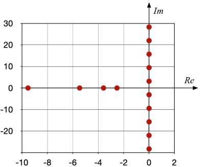
We then have the surprising observation that a slight diffusion in the system has, in this case, a clear destabilizing effect. This is graphically illustrated in Figure 6 and leads to the following conjecture.

Conjecture 2.

For all ϵ>0italic-ϵ0\epsilon>0, there exists η1>0subscript𝜂10\eta_{1}>0 such that for all η(0,η1)𝜂0subscript𝜂1\eta\in(0,\eta_{1}) the maximal spectral abscissa satisfies the inequality ση>ϵsubscript𝜎𝜂italic-ϵ\sigma_{\eta}>-\epsilon. ∎

Refer to caption
Figure 6: The spectrum 𝒮ηsubscript𝒮𝜂\mathcal{S}_{\eta} of the system (96) with η=0.1𝜂0.1\eta=0.1.

7 Conclusion

We have discussed the output feedback stabilization of an unstable open loop system which is made up of two interconnected transport equations and provided with anti-located boundary sensing and actuation. We have shown that the system can be stabilized by a dynamic controller that involves a delayed output feedback which turns out to be non-robust with respect to delay uncertainties. Then we have shown that the designed control law can however stabilize the system in a robust way when there is a small unknown diffusion in the plant.

Our work in progress on this topic [6] will be focused on the output feedback stabilization of the motion of a viscous fluid represented by 2×2222\times 2 hyperbolic PDEs when the control input is the flow rate at one boundary while the measurable output is the fluid density at the other boundary. There is, in this case, an important difference which lies in how viscosity affects the model, inducing a distributed internal coupling between the two partial differential equations. This implies that the system can no longer be considered as a feedback interconnection of two independent scalar transport equations which may lead to additional difficulties for the stability analysis.

Acknowledgement

The authors would like to thank the Bernoulli center for fundamental studies (CIB) and Joachim Krieger for their hospitality and their support, as well as the projet PEPS JCJC 2022 of CNRS - INSMI.

References

  • [1] O-M. Aamo. Disturbance rejection in 2 ×\times 2 linear hyperbolic systems. IEEE Transactions on Automatic Control, 58(5):1095–1106, May 2013.
  • [2] H. Anfinsen and O-M. Aamo. Adaptive output-feedback stabilization of linear 2 ×\times 2 hyperbolic systems using anti-collocated sensing and control. Systems and Control Letters, 104:86–94, 2017.
  • [3] H. Anfinsen and O-M. Aamo. Disturbance rejection in general heterodirectional 1-d linear hyperbolic systems using collocated sensing and control. Automatica, 76:230–242, 2017.
  • [4] J. Auriol and F. Di Meglio. Minimum time control of heterodirectional linear coupled hyperbolic PDEs. Automatica, 71:300–307, 2016.
  • [5] G. Bastin and J-M. Coron. Stability and Boundary Stabilisation of 1-D Hyperbolic Systems. Number 88 in Progress in Nonlinear Differential Equations and Their Applications. Springer International, 2016.
  • [6] G. Bastin, J-M. Coron, and A. Hayat. The usefulness of diffusion for the robustness of boundary output feedback control of an unstable fluid system. Work in progress, 2022.
  • [7] P. Bernard and M. Krstic. Adaptive output-feedback stabilization of non-local hyperbolic PDEs. Automatica, 50:2692–2699, 2014.
  • [8] Y. Chitour, G. Mazanti, and M. Sigalotti. Stability of non-autonomous difference equations with applications to transport and wave propagation on networks. Netw. Heterog. Media, 11(4):563–601, 2016.
  • [9] J-M. Coron, G. Bastin, and B. d’Andréa-Novel. Dissipative boundary conditions for one dimensional nonlinear hyperbolic systems. SIAM Journal of Control and Optimization, 47(3):1460–1498, 2008.
  • [10] V. Dos Santos Martins and C. Prieur. Boundary control of open channels with numerical and experimental validations. IEEE Transactions on Control Systems Technology, 16(6):1252–1264, 2008.
  • [11] C. Franco and J. Collado. Ziegler paradox and periodic coefficient differential equations. In Proceedings 12th International Conference on Electrical Engineering, Computing Science and Automatic Control (CCE), pages 1–5, 2015.
  • [12] E. Fridman. Introduction to time-delay systems: Analysis and control. Springer, 2014.
  • [13] M. Gugat. Optimal Boundary Control and Boundary Stabilization of Hyperbolic Systems. SpringerBriefs in Electrical and Computer Engineering. Springer, 2015.
  • [14] M. Gugat, G. Leugering, S. Tamasoiu, and K. Wang. H2superscript𝐻2{H}^{2}-stabilization of the isothermal euler equations: a Lyapunov function approach. Chinese Annals of Mathematics. Series B, 33(4):479–500, 2012.
  • [15] J.K. Hale and S.M. Verduyn-Lunel. Introduction to Functional-Differential Equations. Number 99 in Appl. Math. Sci. Springer-Verlag, New York, 1993.
  • [16] A. Hayat and P. Shang. A quadratic Lyapunov function for Saint-Venant equations with arbitrary friction and space-varying slope. Automatica, 100:52–60, 2019.
  • [17] L. Hu, F. Di Meglio, R. Vazquez, and M. Krstic. Control of homodirectional and general heterodirectional linear coupled hyperbolic PDEs. IEEE Transactions on Automatic Control, 61(11):3301–3314, 2016.
  • [18] M. Krstic, B-Z. Guo, A. Balogh, and A. Smyshlyaev. Output-feedback stabilization of an unstable wave equation. Automatica, 44:63–74, 2008.
  • [19] M. Lichtner. Spectral mapping theorem for linear hyperbolic systems. Proceedings of the American Mathematical Society, 136(6):2091–2101, 2008.
  • [20] W. Michiels and S-I. Niculescu. Stability and Stabilization of Time-Delay Systems. Advances in Design and Control 12. SIAM, Philadelphia, 2007.
  • [21] R.A. Silkowski. Star Shaped Regions of Stability in Hereditary Systems. PhD thesis, Brown University, Providence, R.I., June 1976.
  • [22] A.M. Turing. The chemical basis of morphogenesis. Philosophical Transactions of the Royal Society B, 237(641):37–72, 1952.
  • [23] J. Wurm, L. Mayer, and F. Woittenek. Feedback control of water waves in a tube with moving boundary. European Journal of Control, 62:151–157, 2021.

Appendix A Computation of ρ¯(𝐊)1¯𝜌𝐊1\bar{\rho}(\mathbf{K})\geqslant 1.

In this appendix we consider the matrix 𝐊𝐊\mathbf{K} defined in equation (15d) as follows:

𝐊=(2k11k2100 100).𝐊matrix2subscript𝑘11subscript𝑘2100100\mathbf{K}=\begin{pmatrix}-2k_{1}&1&-k_{2}\\[5.0pt] 1&0&0\\[5.0pt] \ 1&0&0\end{pmatrix}. (101)

From [9, Proposition 3.7] and [5, Theorem 3.12], we have

ρ¯(K)=ρ2(K)¯𝜌𝐾subscript𝜌2𝐾\bar{\rho}(K)=\rho_{2}(K) (102)

with

ρ2(𝐊)subscript𝜌2𝐊\displaystyle\rho_{2}(\mathbf{K}) :=inf{D𝐊D12;D is a positive diagonal matrix}assignabsentinfimumsubscriptnorm𝐷𝐊superscript𝐷12𝐷 is a positive diagonal matrix\displaystyle:=\inf\{\|D\mathbf{K}D^{-1}\|_{2};D\text{ is a positive diagonal matrix}\} (103)
=inf{λmax[(D𝐊D1)T(D𝐊D1)];D is a positive diagonal matrix}.absentinfimumsubscript𝜆delimited-[]superscript𝐷𝐊superscript𝐷1𝑇𝐷𝐊superscript𝐷1𝐷 is a positive diagonal matrix\displaystyle=\inf\left\{\sqrt{\lambda_{\max}\big{[}\big{(}D\mathbf{K}D^{-1}\big{)}^{T}\big{(}D\mathbf{K}D^{-1}\big{)}\big{]}};D\text{ is a positive diagonal matrix}\right\}. (104)

With the (normalized) matrix

D=(1000θ2000θ3),θ2>0,θ3>0,formulae-sequence𝐷matrix1000subscript𝜃2000subscript𝜃3formulae-sequencesubscript𝜃20subscript𝜃30D=\begin{pmatrix}1&0&0\\ 0&\theta_{2}&0\\ 0&0&\theta_{3}\end{pmatrix},\hskip 14.22636pt\theta_{2}>0,\;\theta_{3}>0, (105)

we have

=(D𝐊D1)T(D𝐊D1)=(4k12+θ22+θ322k1θ212k1k2θ312k1θ21θ22k2θ21θ312k1k2θ31k2θ21θ31k22θ32).superscript𝐷𝐊superscript𝐷1𝑇𝐷𝐊superscript𝐷1matrix4superscriptsubscript𝑘12superscriptsubscript𝜃22superscriptsubscript𝜃322subscript𝑘1superscriptsubscript𝜃212subscript𝑘1subscript𝑘2superscriptsubscript𝜃312subscript𝑘1superscriptsubscript𝜃21superscriptsubscript𝜃22subscript𝑘2superscriptsubscript𝜃21superscriptsubscript𝜃312subscript𝑘1subscript𝑘2superscriptsubscript𝜃31subscript𝑘2superscriptsubscript𝜃21superscriptsubscript𝜃31superscriptsubscript𝑘22superscriptsubscript𝜃32\mathcal{M}=\big{(}D\mathbf{K}D^{-1}\big{)}^{T}\big{(}D\mathbf{K}D^{-1}\big{)}=\begin{pmatrix}4k_{1}^{2}+\theta_{2}^{2}+\theta_{3}^{2}&-2k_{1}\theta_{2}^{-1}&2k_{1}k_{2}\theta_{3}^{-1}\\[5.0pt] -2k_{1}\theta_{2}^{-1}&\theta_{2}^{-2}&-k_{2}\theta_{2}^{-1}\theta_{3}^{-1}\\[5.0pt] 2k_{1}k_{2}\theta_{3}^{-1}&-k_{2}\theta_{2}^{-1}\theta_{3}^{-1}&k_{2}^{2}\theta_{3}^{-2}\end{pmatrix}. (106)

Then we have

det(λ𝐈3)=λ(λ2βλ+γ)𝜆subscript𝐈3𝜆superscript𝜆2𝛽𝜆𝛾\det\big{(}\lambda\mathbf{I}_{3}-\mathcal{M}\big{)}=\lambda(\lambda^{2}-\beta\lambda+\gamma) (107)

with

β=4k12+(θ22+θ22)+(θ32+k22θ32),𝛽4superscriptsubscript𝑘12superscriptsubscript𝜃22superscriptsubscript𝜃22superscriptsubscript𝜃32superscriptsubscript𝑘22superscriptsubscript𝜃32\displaystyle\beta=4k_{1}^{2}+(\theta_{2}^{2}+\theta_{2}^{-2})+(\theta_{3}^{2}+k_{2}^{2}\theta_{3}^{-2}), (108)
γ=1+θ22θ32+k22+k22θ22θ32.𝛾1superscriptsubscript𝜃22superscriptsubscript𝜃32superscriptsubscript𝑘22superscriptsubscript𝑘22superscriptsubscript𝜃22superscriptsubscript𝜃32\displaystyle\gamma=1+\theta_{2}^{-2}\theta_{3}^{2}+k_{2}^{2}+k_{2}^{2}\theta_{2}^{2}\theta_{3}^{-2}. (109)

From (107) we see that the eigenvalues of the matrix \mathcal{M} are

λ=0andλ=β±β24γ2.formulae-sequence𝜆0and𝜆plus-or-minus𝛽superscript𝛽24𝛾2\lambda=0\hskip 14.22636pt\text{and}\hskip 14.22636pt\lambda=\dfrac{\beta\pm\sqrt{\beta^{2}-4\gamma}}{2}. (110)

From (108) we know that β0𝛽0\beta\geqslant 0. Moreover, β24γ0superscript𝛽24𝛾0\beta^{2}-4\gamma\geqslant 0 because the matrix \mathcal{M} is symmetric. It follows that

ρ2(𝐊)=infθ2,θ3β+β24γ2.subscript𝜌2𝐊subscriptinfimumsubscript𝜃2subscript𝜃3𝛽superscript𝛽24𝛾2\displaystyle\rho_{2}(\mathbf{K})=\inf_{\theta_{2},\theta_{3}}\sqrt{\dfrac{\beta+\sqrt{\beta^{2}-4\gamma}}{2}}. (111)

From (108) and (109), after some computations, we get

β24γ=16k14+8k12(θ22+θ22)+8k12(θ32+k22θ32)+(θ24+θ24)+(θ34+k24θ34)+2(θ22θ32+k22θ22θ32)22k222(θ22θ32+k22θ22θ32).superscript𝛽24𝛾16superscriptsubscript𝑘148superscriptsubscript𝑘12superscriptsubscript𝜃22superscriptsubscript𝜃228superscriptsubscript𝑘12superscriptsubscript𝜃32superscriptsubscript𝑘22superscriptsubscript𝜃32superscriptsubscript𝜃24superscriptsubscript𝜃24superscriptsubscript𝜃34superscriptsubscript𝑘24superscriptsubscript𝜃342superscriptsubscript𝜃22superscriptsubscript𝜃32superscriptsubscript𝑘22superscriptsubscript𝜃22superscriptsubscript𝜃3222superscriptsubscript𝑘222superscriptsubscript𝜃22superscriptsubscript𝜃32superscriptsubscript𝑘22superscriptsubscript𝜃22superscriptsubscript𝜃32\beta^{2}-4\gamma=16\,k_{1}^{4}+8k_{1}^{2}(\theta_{2}^{2}+\theta_{2}^{-2})+8k_{1}^{2}(\theta_{3}^{2}+k_{2}^{2}\theta_{3}^{-2})+(\theta_{2}^{4}+\theta_{2}^{-4})+(\theta_{3}^{4}+k_{2}^{4}\theta_{3}^{-4})\\[5.0pt] +2(\theta_{2}^{2}\theta_{3}^{2}+k_{2}^{2}\theta_{2}^{-2}\theta_{3}^{-2})-2-2k_{2}^{2}-2(\theta_{2}^{-2}\theta_{3}^{2}+k_{2}^{2}\theta_{2}^{2}\theta_{3}^{-2}). (112)

From (108) and this latter expression it can be verified that β+β24γ𝛽superscript𝛽24𝛾\beta+\sqrt{\beta^{2}-4\gamma} is minimal if and only if

θ22=1andθ32=|k2|.formulae-sequencesuperscriptsubscript𝜃221andsuperscriptsubscript𝜃32subscript𝑘2\theta_{2}^{2}=1\hskip 14.22636pt\text{and}\hskip 14.22636pt\theta_{3}^{2}=|k_{2}|. (113)

With these values we then have

ρ2(𝐊)subscript𝜌2𝐊\displaystyle\rho_{2}(\mathbf{K}) =infθ2,θ3β+β24γ2absentsubscriptinfimumsubscript𝜃2subscript𝜃3𝛽superscript𝛽24𝛾2\displaystyle=\inf_{\theta_{2},\theta_{3}}\sqrt{\dfrac{\beta+\sqrt{\beta^{2}-4\gamma}}{2}} (114)
=|k1|+1+k12+|k2|1for all(k1,k2).formulae-sequenceabsentsubscript𝑘11superscriptsubscript𝑘12subscript𝑘21for allsubscript𝑘1subscript𝑘2\displaystyle=|k_{1}|+\sqrt{1+k_{1}^{2}+|k_{2}|}\;\;\geqslant 1\hskip 14.22636pt\text{for all}\;(k_{1},k_{2}). (115)

Appendix B Proof of Lemma 1.

Part a)

Assume by contradiction that Re(z¯2)(1,+]Resuperscript¯𝑧21\text{Re}(\bar{z}^{2})\in(1,+\infty]. Then

e(Re(zn2)1)/4ηn0superscript𝑒Resuperscriptsubscript𝑧𝑛214subscript𝜂𝑛0e^{-(\text{Re}(z_{n}^{2})-1)/4\eta_{n}}\longrightarrow 0 (116)

and it follows that the right-hand side of (43) converges to ±2plus-or-minus2\pm 2. Then, denoting an=Re(zn)subscript𝑎𝑛Resubscript𝑧𝑛a_{n}=\text{Re}(z_{n}) and bn=Im(zn)subscript𝑏𝑛Imsubscript𝑧𝑛b_{n}=\text{Im}(z_{n}), (43) implies

12((anibnan2+bn2+1)e(1anibn)/2ηn(anibnan2+bn21)e(1+an+ibn)/2ηn)±1.12subscript𝑎𝑛𝑖subscript𝑏𝑛superscriptsubscript𝑎𝑛2superscriptsubscript𝑏𝑛21superscript𝑒1subscript𝑎𝑛𝑖subscript𝑏𝑛2subscript𝜂𝑛subscript𝑎𝑛𝑖subscript𝑏𝑛superscriptsubscript𝑎𝑛2superscriptsubscript𝑏𝑛21superscript𝑒1subscript𝑎𝑛𝑖subscript𝑏𝑛2subscript𝜂𝑛plus-or-minus1\frac{1}{2}\left(\left(\frac{a_{n}-ib_{n}}{a_{n}^{2}+b_{n}^{2}}+1\right)e^{-(1-a_{n}-ib_{n})/2\eta_{n}}-\left(\frac{a_{n}-ib_{n}}{a_{n}^{2}+b_{n}^{2}}-1\right)e^{-(1+a_{n}+ib_{n})/2\eta_{n}}\right)\rightarrow\pm 1. (117)

Since Re(z¯2)(1,+]Resuperscript¯𝑧21\text{Re}(\bar{z}^{2})\in(1,+\infty] by assumption, it follows that there exists a positive constant c𝑐c such that an2>c+1+bn2superscriptsubscript𝑎𝑛2𝑐1superscriptsubscript𝑏𝑛2a_{n}^{2}>c+1+b_{n}^{2} for n𝑛n sufficiently large, and in particular that |Re(z¯)|>1Re¯𝑧1|\text{Re}(\bar{z})|>1. Let us consider successively the two possibilities Re(z¯)>1Re¯𝑧1\text{Re}(\bar{z})>1 and Re(z¯)<1Re¯𝑧1\text{Re}(\bar{z})<-1.

The case Re(𝐳¯)>𝟏.Re¯𝐳1\mathbf{\text{Re}(\bar{z})>1.}

In this case, if n𝑛n is sufficiently large, we have

Re(anibnan2+bn2+1)1ande(an1)/2ηn+.formulae-sequenceResubscript𝑎𝑛𝑖subscript𝑏𝑛superscriptsubscript𝑎𝑛2superscriptsubscript𝑏𝑛211andsuperscript𝑒subscript𝑎𝑛12subscript𝜂𝑛\text{Re}\left(\frac{a_{n}-ib_{n}}{a_{n}^{2}+b_{n}^{2}}+1\right)\geq 1\hskip 14.22636pt\text{and}\hskip 14.22636pte^{(a_{n}-1)/2\eta_{n}}\longrightarrow+\infty. (118)

Thus

|12(anibnan2+bn2+1)e(an1)/2ηn|+,12subscript𝑎𝑛𝑖subscript𝑏𝑛superscriptsubscript𝑎𝑛2superscriptsubscript𝑏𝑛21superscript𝑒subscript𝑎𝑛12subscript𝜂𝑛\left|\frac{1}{2}\left(\frac{a_{n}-ib_{n}}{a_{n}^{2}+b_{n}^{2}}+1\right)e^{(a_{n}-1)/2\eta_{n}}\right|\longrightarrow+\infty, (119)

while

12(anibnan2+bn21)e(an1)/2ηneibn/2ηn0.12subscript𝑎𝑛𝑖subscript𝑏𝑛superscriptsubscript𝑎𝑛2superscriptsubscript𝑏𝑛21superscript𝑒subscript𝑎𝑛12subscript𝜂𝑛superscript𝑒𝑖subscript𝑏𝑛2subscript𝜂𝑛0\frac{1}{2}\left(\frac{a_{n}-ib_{n}}{a_{n}^{2}+b_{n}^{2}}-1\right)e^{(-a_{n}-1)/2\eta_{n}}e^{-ib_{n}/2\eta_{n}}\longrightarrow 0. (120)

This implies

|12(anibnan2+bn2+1)e(an1)/2ηneibn/2ηn12(anibnan2+bn21)e(1+an+ibn)/2ηn|+,12subscript𝑎𝑛𝑖subscript𝑏𝑛superscriptsubscript𝑎𝑛2superscriptsubscript𝑏𝑛21superscript𝑒subscript𝑎𝑛12subscript𝜂𝑛superscript𝑒𝑖subscript𝑏𝑛2subscript𝜂𝑛12subscript𝑎𝑛𝑖subscript𝑏𝑛superscriptsubscript𝑎𝑛2superscriptsubscript𝑏𝑛21superscript𝑒1subscript𝑎𝑛𝑖subscript𝑏𝑛2subscript𝜂𝑛\left|\frac{1}{2}\left(\frac{a_{n}-ib_{n}}{a_{n}^{2}+b_{n}^{2}}+1\right)e^{(a_{n}-1)/2\eta_{n}}e^{ib_{n}/2\eta_{n}}-\frac{1}{2}\left(\frac{a_{n}-ib_{n}}{a_{n}^{2}+b_{n}^{2}}-1\right)e^{-(1+a_{n}+ib_{n})/2\eta_{n}}\right|\longrightarrow+\infty, (121)

which is in contradiction with (117).

The case Re(𝐳¯)<𝟏.Re¯𝐳1\mathbf{\text{Re}(\bar{z})<-1.}

Similarly in this case we have

e(an1)/2ηn+and|(anibnan2+bn21)e(an1)/2ηneibn/2ηn|+,formulae-sequencesuperscript𝑒subscript𝑎𝑛12subscript𝜂𝑛andsubscript𝑎𝑛𝑖subscript𝑏𝑛superscriptsubscript𝑎𝑛2superscriptsubscript𝑏𝑛21superscript𝑒subscript𝑎𝑛12subscript𝜂𝑛superscript𝑒𝑖subscript𝑏𝑛2subscript𝜂𝑛e^{(-a_{n}-1)/2\eta_{n}}\longrightarrow+\infty\hskip 14.22636pt\text{and}\hskip 14.22636pt\left|\left(\frac{a_{n}-ib_{n}}{a_{n}^{2}+b_{n}^{2}}-1\right)e^{(-a_{n}-1)/2\eta_{n}}e^{-ib_{n}/2\eta_{n}}\right|\longrightarrow+\infty, (122)

while

|12(anibnan2+bn2+1)e(an1)/2ηneibn/2ηn|0.12subscript𝑎𝑛𝑖subscript𝑏𝑛superscriptsubscript𝑎𝑛2superscriptsubscript𝑏𝑛21superscript𝑒subscript𝑎𝑛12subscript𝜂𝑛superscript𝑒𝑖subscript𝑏𝑛2subscript𝜂𝑛0\left|\frac{1}{2}\left(\frac{a_{n}-ib_{n}}{a_{n}^{2}+b_{n}^{2}}+1\right)e^{(a_{n}-1)/2\eta_{n}}e^{ib_{n}/2\eta_{n}}\right|\longrightarrow 0. (123)

So we get again (121) and a contradiction with (117). This concludes the proof of Lemma 1, Part a).

Part b)

We assume that

Re(z¯2)=1.Resuperscript¯𝑧21\text{Re}(\bar{z}^{2})=1. (124)

We have

Re(z¯2)=(Re(z¯))2(Im(z¯))2.Resuperscript¯𝑧2superscriptRe¯𝑧2superscriptIm¯𝑧2\text{Re}(\bar{z}^{2})=\big{(}\text{Re}(\bar{z})\big{)}^{\!2}-\big{(}\text{Im}(\bar{z})\big{)}^{\!2}. (125)

From this expression and (124), either |Re(z¯)|=1Re¯𝑧1|\text{Re}(\bar{z})|=1 and Im(z¯)=0Im¯𝑧0\text{Im}(\bar{z})=0, or |Re(z¯)|>1Re¯𝑧1|\text{Re}(\bar{z})|>1.

We shall show by contradiction that |Re(z¯)|>1Re¯𝑧1|\text{Re}(\bar{z})|>1 is actually not possible. Let us thus assume that Re(z¯)>1Re¯𝑧1\text{Re}(\bar{z})>1 (the case Re(z¯)<1Re¯𝑧1\text{Re}(\bar{z})<-1 can be easily handled by symmetry). In that case, using again the notations an=Re(zn)subscript𝑎𝑛Resubscript𝑧𝑛a_{n}=\text{Re}(z_{n}) and bn=Im(zn)subscript𝑏𝑛Imsubscript𝑧𝑛b_{n}=\text{Im}(z_{n}) and multiplying both sides of (43) by e(1an)/4ηnsuperscript𝑒1subscript𝑎𝑛4subscript𝜂𝑛e^{(1-a_{n})/4\eta_{n}}, we obtain:

(anibnan2+bn2+1)e(an1)/4ηn+ibn/2ηn(anibnan2+bn21)e(1+3an+2ibn)/4ηn=e(2an2+bn2an2ianbn)/4ηn±e(2an2+bn2an2ianbn)/2ηn+4e(1an)/2ηn.subscript𝑎𝑛𝑖subscript𝑏𝑛superscriptsubscript𝑎𝑛2superscriptsubscript𝑏𝑛21superscript𝑒subscript𝑎𝑛14subscript𝜂𝑛𝑖subscript𝑏𝑛2subscript𝜂𝑛subscript𝑎𝑛𝑖subscript𝑏𝑛superscriptsubscript𝑎𝑛2superscriptsubscript𝑏𝑛21superscript𝑒13subscript𝑎𝑛2𝑖subscript𝑏𝑛4subscript𝜂𝑛plus-or-minussuperscript𝑒2superscriptsubscript𝑎𝑛2superscriptsubscript𝑏𝑛2subscript𝑎𝑛2𝑖subscript𝑎𝑛subscript𝑏𝑛4subscript𝜂𝑛superscript𝑒2superscriptsubscript𝑎𝑛2superscriptsubscript𝑏𝑛2subscript𝑎𝑛2𝑖subscript𝑎𝑛subscript𝑏𝑛2subscript𝜂𝑛4superscript𝑒1subscript𝑎𝑛2subscript𝜂𝑛\begin{split}&\left(\frac{a_{n}-ib_{n}}{a_{n}^{2}+b_{n}^{2}}+1\right)e^{(a_{n}-1)/4\eta_{n}+ib_{n}/2\eta_{n}}-\left(\frac{a_{n}-ib_{n}}{a_{n}^{2}+b_{n}^{2}}-1\right)e^{-(1+3a_{n}+2ib_{n})/4\eta_{n}}\\[5.0pt] &=-e^{(2-a_{n}^{2}+b_{n}^{2}-a_{n}-2ia_{n}b_{n})/4\eta_{n}}\pm\sqrt{e^{(2-a_{n}^{2}+b_{n}^{2}-a_{n}-2ia_{n}b_{n})/2\eta_{n}}+4e^{(1-a_{n})/2\eta_{n}}}.\end{split} (126)

Since

1an1Re(z¯)<01subscript𝑎𝑛1Re¯𝑧01-a_{n}\rightarrow 1-\text{Re}(\bar{z})<0 (127)

and, by (124), 2an2+bn2an1Re(z¯)<02superscriptsubscript𝑎𝑛2superscriptsubscript𝑏𝑛2subscript𝑎𝑛1Re¯𝑧02-a_{n}^{2}+b_{n}^{2}-a_{n}\rightarrow 1-\text{Re}(\bar{z})<0, the right-hand side of (126) converges to 0 when ηn0+subscript𝜂𝑛superscript0\eta_{n}\rightarrow 0^{+}. This implies that the left-hand side of (126) also converges to 0, namely

(anibnan2+bn2+1)e(an1)/4ηn+ibn/2ηn(anibnan2+bn21)e(1+3an+2ibn)/4ηn0.subscript𝑎𝑛𝑖subscript𝑏𝑛superscriptsubscript𝑎𝑛2superscriptsubscript𝑏𝑛21superscript𝑒subscript𝑎𝑛14subscript𝜂𝑛𝑖subscript𝑏𝑛2subscript𝜂𝑛subscript𝑎𝑛𝑖subscript𝑏𝑛superscriptsubscript𝑎𝑛2superscriptsubscript𝑏𝑛21superscript𝑒13subscript𝑎𝑛2𝑖subscript𝑏𝑛4subscript𝜂𝑛0\left(\frac{a_{n}-ib_{n}}{a_{n}^{2}+b_{n}^{2}}+1\right)e^{(a_{n}-1)/4\eta_{n}+ib_{n}/2\eta_{n}}-\left(\frac{a_{n}-ib_{n}}{a_{n}^{2}+b_{n}^{2}}-1\right)e^{-(1+3a_{n}+2ib_{n})/4\eta_{n}}\rightarrow 0. (128)

Then, since the e(1+3an+ibn)/2ηn0superscript𝑒13subscript𝑎𝑛𝑖subscript𝑏𝑛2subscript𝜂𝑛0e^{-(1+3a_{n}+ib_{n})/2\eta_{n}}\rightarrow 0, we should have

|(anibnan2+bn2+1)|e(an1)/4ηn0,subscript𝑎𝑛𝑖subscript𝑏𝑛superscriptsubscript𝑎𝑛2superscriptsubscript𝑏𝑛21superscript𝑒subscript𝑎𝑛14subscript𝜂𝑛0\left|\left(\frac{a_{n}-ib_{n}}{a_{n}^{2}+b_{n}^{2}}+1\right)\right|e^{(a_{n}-1)/4\eta_{n}}\rightarrow 0, (129)

but it can be shown that this is impossible. Indeed, by (127), we know that an>0subscript𝑎𝑛0a_{n}>0 if n𝑛n is large enough, which implies that

|(anibnan2+bn2+1)|e(an1)/4ηne(an1)/4ηn.subscript𝑎𝑛𝑖subscript𝑏𝑛superscriptsubscript𝑎𝑛2superscriptsubscript𝑏𝑛21superscript𝑒subscript𝑎𝑛14subscript𝜂𝑛superscript𝑒subscript𝑎𝑛14subscript𝜂𝑛\left|\left(\frac{a_{n}-ib_{n}}{a_{n}^{2}+b_{n}^{2}}+1\right)\right|e^{(a_{n}-1)/4\eta_{n}}\geqslant e^{(a_{n}-1)/4\eta_{n}}. (130)

From (127), e(an1)4η+superscript𝑒subscript𝑎𝑛14𝜂e^{\frac{(a_{n}-1)}{4\eta}}\rightarrow+\infty which leads to a contradiction with (129) and (130).

This concludes the proof of Lemma 1. ∎