AUC Maximization for Low-Resource Named Entity Recognition

Abstract

Current work in named entity recognition (NER) uses either cross entropy (CE) or conditional random fields (CRF) as the objective/loss functions to optimize the underlying NER model. Both of these traditional objective functions for the NER problem generally produce adequate performance when the data distribution is balanced and there are sufficient annotated training examples. But since NER is inherently an imbalanced tagging problem, the model performance under the low-resource settings could suffer using these standard objective functions. Based on recent advances in area under the ROC curve (AUC) maximization, we propose to optimize the NER model by maximizing the AUC score. We give evidence that by simply combining two binary-classifiers that maximize the AUC score, significant performance improvement over traditional loss functions is achieved under low-resource NER settings. We also conduct extensive experiments to demonstrate the advantages of our method under the low-resource and highly-imbalanced data distribution settings. To the best of our knowledge, this is the first work that brings AUC maximization to the NER setting. Furthermore, we show that our method is agnostic to different types of NER embeddings, models and domains. The code of this work is available at https://github.com/dngu0061/NER-AUC-2T.

Introduction

Named Entity Recognition (NER) is a fundamental NLP task which aims to locate named entity (NE) mentions and classify them into predefined categories such as location, organization, or person. NER usually serves as an important sub-task for information extraction (Ritter, Etzioni, and Clark 2012), information retrieval (Banerjee et al. 2019), task oriented dialogues (Peng et al. 2021), knowledge base construction (Etzioni et al. 2005) and other language applications. Recently, NER has gained significant performance improvements with the advances of pre-trained language models (PLMs) (Devlin et al. 2019). Unfortunately, a large amount of training data is often essential for these PLMs to excel and except for a few high-resource domains, the majority of domains (e.g., biomedical domain) are scarce and have limited amount of labeled data (Giorgi and Bader 2019).

Figure 1: Reformulating the traditional multi-class NER-tagging problem as a two-task learning problem. The first task is to detect if a word is inside an NE, while the second task is to detect if a word is at the beginning of an NE.

Since manually annotating a large amount of data in each domain or language is expensive, time-consuming, and often infeasible without domain expertise (e.g., biomedical NER) (Tan, Du, and Buntine 2021; Nguyen et al. 2022), machine learning practitioners have focused on other alternative approaches to produce effective solution to overcome this data scarcity issue. These approaches include data augmentation (Etzioni et al. 2005; Chen et al. 2021; Zhou et al. 2022), domain adaptation (Li, Shang, and Shao 2020), and multilingual transfers (Rahimi, Li, and Cohn 2019). Although these approaches have shown promising results, they ignore the highly imbalanced data distribution that is inherent to NER corpora. Table 1 summarizes this issue. While the imbalanced data distribution issue exists in both CoNLL 2003 (Tjong Kim Sang and De Meulder 2003) and OntoNotes5 (Weischedel et al. 2014) where the majority of tag is “O”, this imbalance issue amplifies given the context of biomedical NER (bioNER). For instance, LINNAEUS (Gerner, Nenadic, and Bergman 2010), one of the hardest bioNER tasks, has nearly 99 percent of its tokens tagged as “O”. Given adequate annotated training examples, the NER model could overcome this issue and learn to classify the tokens correctly. Nonetheless, many corpora, especially those from the biomedical domain, can be scarcely labeled.

Since NER corpora can be both scarcely labeled and highly imbalanced, we argue that the standard cross entropy objective function, though capable of producing the optimal token classifier asymptotically under the maximum likelihood principle, would fail to achieve the desirable performance under the low-resource and imbalanced settings.

Dataset # sentences # tokens % label (B/I/O) Train Dev Test Train Dev Test Train Dev Test CoNLL 2003 (2003) 14,987 3,466 3,684 203,621 51,362 46,435 11.5 5.2 83.3 11.5 5.2 83.3 12.2 5.3 82.5 OntoNotes5 (2014) 20,000 3,000 3,000 364,611 54,423 55,827 6.2 4.9 89.1 6.2 4.9 89.1 6.1 4.9 89.0 LINNAEUS (2010) 11,934 4,077 7,141 281,273 93,877 165,095 0.7 0.4 98.9 0.8 0.4 98.8 0.9 0.5 98.6 NCBI (2014) 5,423 922 939 135,701 23,969 24,497 3.8 4.5 91.7 3.3 4.5 92.2 3.9 4.4 91.7 s800 (2013) 5,732 829 1,629 147,291 22,217 42,298 1.7 2.2 96.1 1.7 2.2 96.1 1.8 2.5 95.7

Table 1: The size of the benchmark NER/bioNER corpora as well as the label distribution for each corpus. In this work, we use the well-defined BIO tagging scheme, i.e., B-Begin, I-Inside, and O-Outside of NEs.

With the above desiderata, this paper considers optimizing the NER model under a different objective/loss function. Instead of optimizing the NER model using the standard cross entropy loss, we propose to optimize the model using the area under ROC curve (AUC) score. Direct optimization of the AUC score has been shown to greatly benefit the performance of highly imbalanced tasks since maximizing AUC aims to rank the prediction score of any positive data higher than that of any negative data (Ying, Wen, and Lyu 2016; Yuan et al. 2021b). However, most recent robust/practical AUC maximization techniques are solely designed to solve for the binary classification task. Thus, this makes direct AUC optimization implementation infeasible for NER. Consequently, we propose to turn the standard BIO tagging problem into a two-task problem. Figure 1 shows how the standard BIO tagging scheme can be converted into two separate tasks, each of which can be optimized with AUC score. At prediction time, the predictions of the two tasks can be combined to generate the final prediction that matches the output normally expected by the BIO tagging scheme.

To demonstrate the effectiveness of our proposed method, we conduct extensive empirical studies on the corpora listed in Table 1. The corpora are from both generic domains, e.g., CoNLL 2003 and OntoNotes5, and specialized domains, e.g., LINNAEUS, NCBI and s800. Using corpora from different domains would substantiate that our method is domain agnostic. Additionally, employing different model architecture such as transformers BERT (Devlin et al. 2019) and seq2seq BART (Lewis et al. 2020) would indicate that our method is model agnostic. Lastly, by experimenting with different pre-trained embeddings, we give evidence that our method is embedding agnostic. Our studies reveals that our method exhibits significant performance improvement over the standard objective/loss functions by a large margin.

We summarize our contributions as follows:

• Two-task NER reformulation: We reformulate the standard NER multi-class approach as a two-task learning problem. Under this new setting, two binary classifiers are used to predict respectively if a word is inside an NE and if a word is at the start of an NE. This simple reformulation makes the AUC optimization feasible for NER.

• A new AUC loss for NER: Instead of optimising the standard loss functions, we adapt the idea of AUC maximization to tackle the lower-resource and imbalanced NER.

• Comprehensive experiments: We conduct extensive empirical studies of our method on a broad range of settings, and demonstrate its consistently strong performance compared with the standard objective functions.

Backgrounds

Named Entity Recognition

NER is a key task in NLP systems such as question-answering, information-retrieval, co-reference resolution, and topic modelling (Yadav and Bethard 2018). Although there are many variations regarding the definition of named entity (NE), the following types remain prevalent 1) generic NEs (e.g., person, organization, and location), and 2) domain-specific NEs (e.g., virus, protein, and genome) (Li et al. 2020; Kripke 1980). For instance, the NER task includes but is not limited to the identification of person, location, or organization in either short or long unstructured texts. In biomedical domains, bioNER is to properly classify virus/disease names into predefined categories. Given a set of tokens $\mathbf{x}=\{x_{1},\ldots,x_{l}\}$, the algorithm would output a list of appropriate tags $\mathbf{y}=\{y_{1},\ldots,y_{l}\}$ (Li et al. 2020). NER is considered a challenging task for two reasons (Lample et al. 2016): 1) in most languages and domains, the amount of manually labeled training data for NER is limited; and 2) it is difficult to generalize from a small sample of training data due to the inherent imbalance nature of NER.

AUC Maximization

AUC (Area Under ROC Curve) has been used in various machine learning works as an important measuring criterion (Freund et al. 2003; Kotlowski, Dembczynski, and Huellermeier 2011; Zuva and Zuva 2012). Since AUC is non-convex, discontinuous and sensitive to model change, direct optimization of AUC score often leads to an NP-hard problem (Yuan et al. 2021b). Thus, many works have tried to alleviate the computational difficulties by providing solutions through a pairwise surrogate loss (Freund et al. 2003), a hinge loss (Zhao et al. 2011), and a least square loss (Gao et al. 2013). Yuan et al. (2021b) pointed out that although the proposed least-square surrogate loss (Gao et al. 2013; Liu et al. 2020) makes AUC maximization scalable, it has two largely ignored issues which are 1) it has an adverse effect when trained with well-classified data (i.e., easy data), and 2) it is sensitive to noisily labeled data (i.e., noisy data). Thus, they proposed to decompose this surrogate least-square loss by what they call AUC margin loss and achieved the 1st place on Stanford CheXpert competition. Further improvements to AUC optimization have been observed via compositional training (Yuan et al. 2021a), i.e., alternating between the cross entropy loss and the AUC surrogate loss during training. AUC maximization works well when 1) there exists an imbalanced data distribution, e.g., classification of chest x-ray images to identify rare threatening diseases, or classification of mammogram for breast cancer study (Yuan et al. 2021b); or 2) the AUC score is the default metric for evaluating and comparing different methods, i.e., directly maximizing AUC score can lead to large improvement in the model performance (Yuan et al. 2021b).

AUX Maximization for NER

Notation

We will use common notation found in the AUC maximization literature (Zhao et al. 2011; Yuan et al. 2021a, b; Yang et al. 2021) to present the problem of AUC maximization in the context of the NER task. Let $\mathbb{I}(\cdot)$ be an indicator function of a predicate, $[s]_{+}=\max(s,0)$. We denote $\mathcal{S}=\left\{\left(\mathbf{x}_{1},\mathbf{y}_{1}\right),\ldots,\left(\mathbf{x}_{n},\mathbf{y}_{n}\right)\right\}$ as a set of training data, where $\mathbf{x}_{i}={x}_{i}^{1},\ldots,{x}_{i}^{l}$ represents the $i$-th training example (i.e., a sentence of length $l$), while $\mathbf{y}_{i}\in\{\text{B},\text{I},\text{O}\}^{l}$ denotes its corresponding sequence of labels. Additionally, $\mathbf{z}=({x},{y})$ will also be used for ease of reference. Following standard machine learning convention, we use $\mathbf{w}\in\mathbb{R}^{d}$ to represent the parameters of the deep neural network to be learned, and $h_{\mathbf{w}}(\mathbf{x})=h(\mathbf{w},\mathbf{x})$ to denote the objective mapping function $h:\mathcal{X}\rightarrow\mathcal{Y}$. Lastly, the standard approach of deep learning is to define a loss/objective function on individual data by $L(\mathbf{w};\mathbf{x},y)=\ell\left(h_{\mathbf{w}}(\mathbf{x}),\mathbf{y}\right)$, where $\ell(\hat{\mathbf{y}},\mathbf{y})$ is a surrogate loss function of the mis-classification error (e.g., cross-entropy loss, conditional random fields), and to minimize the empirical loss $\min_{\mathbf{w}\in\mathbb{R}^{d}}\frac{1}{n}\sum_{i=1}^{n}L\left(\mathbf{w};\mathbf{x}_{i},\mathbf{y}_{i}\right)$. However, as we previously discussed, this standard surrogate loss function is not suitable for situations where there exists an imbalanced data distribution. This imbalanced data distribution issue is the inherent problem for the NER/bioNER task as most corpora have the majority of labels tagged as “O” (see Table 1).

Reformulation of NER

Existing work on AUC maximization typically follows the Wilcoxon-Mann-Whitney statistic (Hanley and McNeil 1982; Clémençon, Lugosi, and Vayatis 2008; Yuan et al. 2021b) and interprets the $\mathrm{AUC}$ score as the probability of a positive sample ranking higher than a negative sample:

$$\hbox to0.0pt{$\displaystyle\operatorname{AUC}(\mathbf{w})$\hss}\\ &=\;\operatorname{Pr}\left(h_{\mathbf{w}}({x})\geq h_{\mathbf{w}}\left({x}^{\prime}\right)\mid y=1,y^{\prime}=-1\right)\\ =\;\mathbb{E}\left[\mathbb{I}\left(h_{\mathbf{w}}({x})-h_{\mathbf{w}}\left({x}^{\prime}\right)\geq 0\right)\mid y=1,y^{\prime}=-1\right].$$ (1)

With $N_{+}$, and $N_{-}$ denoting the size of positive and negative training data set respectively, many existing works formulate the AUC maximization on training data $\mathcal{S}\equiv\{\mathcal{S}_{-},\mathcal{S}_{+}\}$ as

$$\hbox to0.0pt{$\displaystyle\operatorname*{arg\,max}_{\mathbf{w}\in\mathbb{R}^{d}}\operatorname{AUC}(\mathbf{w})$\hss}\\ &=\operatorname*{arg\,min}_{\mathbf{w}\in\mathbb{R}^{d}}\operatorname{Pr}\left(h_{\mathbf{w}}({x})<h_{\mathbf{w}}\left({x}^{\prime}\right)\mid y=1,y^{\prime}=-1\right)\\ =\operatorname*{arg\,min}_{\mathbf{w}\in\mathbb{R}^{d}}\mathbb{E}\left[\mathbb{I}\left(h_{\mathbf{w}}({x})-h_{\mathbf{w}}\left({x}^{\prime}\right)<0\right)\mid y=1,y^{\prime}=-1\right]\\ \equiv\operatorname*{arg\,min}_{\mathbf{w}\in\mathbb{R}^{d}}\frac{1}{N_{+}N_{-}}\sum_{{x}\in\mathcal{S}_{+}}\sum_{{x}^{\prime}\in\mathcal{S}_{-}}\mathbb{I}\left(h_{\mathbf{w}}({x})-h_{\mathbf{w}}\left({x}^{\prime}\right)<0\right).$$ (2)

While the definition from Eqs (1) and (2) subsequently leads to the development of many prominent works in AUC maximization, it is not directly applicable to the NER problem.

To make direct AUC maximization applicable to NER, we propose to reformulate the standard NER multi-class setting into a two-task setting as shown in Figure 2. In this setting, the standard BIO-tagging scheme is broken into two parallel tasks. One of the tasks is to detect if the token $x_{i}^{l}$ belongs to a named entity, we name the label of this task $\mathbf{y}_{\textbf{en}_{i}}\in\{-1,1\}^{l}$. The other task is to detect if the token $x_{i}^{l}$ is the beginning token of the named entity, we name the label of this task $\mathbf{y}_{\textbf{be}_{i}}\in\{-1,1\}^{l}$, i.e., $\mathbf{y}_{i}=\{\mathbf{y}_{\textbf{en}_{i}},\mathbf{y}_{\textbf{be}_{i}}\}$. Based on this two-task setting, the parameters set $\mathbf{w}$ can be separated into two sets, $\mathbf{w}_{\textbf{en}}=\{\theta,\omega_{\textbf{en}}\}$ and $\mathbf{w}_{\textbf{be}}=\{\theta,\omega_{\textbf{be}}\}$. $\theta$ denotes the shared embedding and language model parameters, while $\omega_{\textbf{en}}$ and $\omega_{\textbf{be}}$ denote the parameters for the entity-token classifier and the beginning-token classifier respectively. By reformulating the standard NER setting into two separate tasks, we can maximize the AUC score of each task. Since the two tasks inherit the imbalanced data distribution problem from the NER multi-class setting, we expect maximizing the AUC score will lead to a better classifier for each task, and eventually improve the NER performance.

Figure 2: Reformulating the traditional multi-class NER-tagging problem as a two-task problem to be optimized with AUC. The embedding and model parameters are shared while the linear classifiers have their own parameter set.

AUC Maximization for NER Two-Task Setting

Although there are many AUC maximization techniques that can be applied to this NER two-task setting, we choose the deep AUC margin loss (DAM) (Yuan et al. 2021b) due to its 1) robustness/scalability of implementation to deep neural networks, and 2) ability to overcome the critics from which previous AUC maximization approaches such as the least-squared surrogate loss might suffer (Ying, Wen, and Lyu 2016; Natole, Ying, and Lyu 2018; Liu et al. 2018, 2020; Yuan et al. 2021b). Under DAM, we define the objective/loss function to the entity-token prediction task as follows:

$$\hbox to0.0pt{$\displaystyle\text{AUC}_{\mathrm{M}}(\mathbf{w}_{\textbf{en}})$\hss}\allowdisplaybreaks\\ &=\mathbb{E}\left[\left(m-h_{\mathbf{w}_{\textbf{en}}}({x})+h_{\mathbf{w}_{\textbf{en}}}\left({x}^{\prime}\right)\right)^{2}\mid y=1,y^{\prime}=-1\right]\allowdisplaybreaks\\ =\min_{a,b}{A_{1}(\mathbf{w}_{\textbf{en}})}+{A_{2}(\mathbf{w}_{\textbf{en}})}+(m-a+b)^{2}\allowdisplaybreaks\\ =\min_{a,b}A_{1}(\mathbf{w}_{\textbf{en}})+A_{2}(\mathbf{w}_{\textbf{en}})+\max_{\alpha\geq 0}\left\{2\alpha(m-a+b)-\alpha^{2}\right\},\allowdisplaybreaks$$ (3)

where $A_{1}(\mathbf{w}_{\textbf{en}})=\mathbb{E}[h^{2}_{\mathbf{w}_{\textbf{en}}}({x})\mid y=1]-a^{2}$, and $A_{2}(\mathbf{w}_{\textbf{en}})=\mathbb{E}[h^{2}_{\mathbf{w}_{\textbf{en}}}({x})\mid y=-1]-b^{2}$. Using the definition for the variance, the minimization problem of $a$ and $b$ is achieved when $a=a(\mathbf{w}_{\textbf{en}})=\mathbb{E}[h_{\mathbf{w}_{\textbf{en}}}({x})\mid y=1]$, and $b=b(\mathbf{w}_{\textbf{en}})=\mathbb{E}[h_{\mathbf{w}_{\textbf{en}}}({x}^{\prime})\mid y=-1]$ respectively. Examining Eq (3) reveals that maximizing AUC requires the predictor 1) to have low variance on both negative and positive words, and 2) to push the mean prediction scores of positive and negative words to be far away based on the value of the margin $m$. We expect that minimizing Eq (3) with respect to $\mathbf{w}_{\textbf{en}}$ can lead to a reliable predictor for the imbalanced entity-token prediction task. Following the same steps, we can define a similar loss function for the beginning-token prediction task. Since this is similar, we will skip this definition in the paper. Lastly, we adhere to the standard multi-task setting and optimize for both tasks by minimizing for the following loss:

$$\text{AUC}_{\mathrm{M}}(\mathbf{w}_{\textbf{en}})+\lambda\text{AUC}_{\mathrm{M}}(\mathbf{w}_{\textbf{be}}),$$ (4)

with $\lambda$ controlling the trade-off between the two losses.

Algorithm 1 NER two-task prediction

Input: $\mathcal{S}_{\text{test}}$, $\mathbf{w}^{*}_{\textbf{en}}$, $\mathbf{w}^{*}_{\textbf{be}}$
Output: $\hat{\mathbf{y}}_{1},\ldots,\hat{\mathbf{y}}_{\text{n-test}}$, s.t., $\hat{\mathbf{y}}_{i}\in\{\text{B, I, O}\}^{l}$

1:  for $\mathbf{x}_{i}\in\mathcal{S}_{\text{test}}$ do

2:     $\hat{\mathbf{y}}_{\textbf{en}_{i}}=h_{\mathbf{w}^{*}_{\textbf{en}}}(\mathbf{x}_{i})$

3:     $\hat{\mathbf{y}}_{\textbf{be}_{i}}=h_{\mathbf{w}^{*}_{\textbf{be}}}(\mathbf{x}_{i})$

4:     for $j$ in range(l) do

5:        if $\hat{{y}}_{\text{en}_{i}}^{j}\equiv 1$ and $\hat{{y}}_{\text{be}_{i}}^{j}\equiv 1$ then

6:           $\hat{{y}}_{i}^{j}:=$ “B”

7:        else if $\hat{{y}}_{\text{en}_{i}}^{j}\equiv 1$ and $\hat{{y}}_{\text{be}_{i}}^{j}\equiv-1$ then

8:           $\hat{{y}}_{i}^{j}:=$ “I”

9:        else

10:           $\hat{{y}}_{i}^{j}:=$ “O”

11:        end if

12:     end for

13:  end for

14:  return $\hat{\mathbf{y}}_{1},\ldots,\hat{\mathbf{y}}_{\text{n-test}}$, s.t., $\hat{\mathbf{y}}_{i}\in\{\text{B, I, O}\}^{l}$

NER Two-Task Prediction

At prediction time, we follow Algorithm 1 to generate the prediction tags expected by the standard BIO-tagging scheme. $\mathbf{w}^{*}_{\textbf{en}}$, and $\mathbf{w}^{*}_{\textbf{be}}$ represent the optimal parameters learnt by minimizing Eq (4) during training. After receiving the predictions from the entity-token and the beginning-token prediction tasks, we linearly combine both sets of predictions to generate the final BIO tags as demonstrated in Algorithm 1. We acknowledge that this linear combination of predictions might raise a certain inconsistency during prediction time when $\hat{{y}}_{\text{en}_{i}}^{j}\equiv-1$ and $\hat{{y}}_{\text{be}_{i}}^{j}\equiv 1$. Currently, we treat the prediction when this happens as “O”. Our justification includes 1) “O” is the major tag for most of the NER corpora (Table 1); thus, predicting “O” would align with the data statistics, and 2) all of the current standard evaluation metrics for NER do not take the true negative prediction into the calculation for the performance score; thus, predicting “O” would lead to no improvement in the evaluation score.

Experimental Settings

We verify the performance of our AUC NER two-task reformulation on both the imbalanced and the low-resource NER settings. All of the experiments were set up as follows.

Domains and Corpora

We used corpora from both the general domain and the biomedical domain. Table 1 summarizes the statistics for these corpora. Both CoNLL 2003 (Tjong Kim Sang and De Meulder 2003) and OntoNotes5 (Weischedel et al. 2014) are standard corpora from the general domain to evaluate and benchmark the NER performance. Whereas NCBI (Doğan, Leaman, and Lu 2014), LINNAEUS (Gerner, Nenadic, and Bergman 2010), and s800 (Pafilis et al. 2013) are standard NER corpora used for biomedical named entity recognition. While NCBI is often used to train the NER model to identify the disease-NEs, both LINNAEUS and s800 are trained to detect species-NEs. Thus, they exhibit different linguistic characteristics. We chose these biomedical corpora to verify the performance of our method since:

• The data distribution of biomedical corpora is often heavily imbalanced, which make them the perfect candidates for AUC maximization in NER. All included biomedical corpora have higher percentage of “O” tag compared to those corpora from the general domain (see Table 1).

• Standard approaches of transferring PLMs from high-resource domains to low-resource ones often fail to achieve satisfactory performance for biomedical corpora (Giorgi and Bader 2019). This happens as clinical narratives can contain challenging linguistic characteristics which do not overlap with those in other domains (Patel et al. 2005), as also observed in our medical NLP project.

By demonstrating the significance of our method over the baselines for both general and specialized domains, it substantiates that our method is both domain and data agnostic.

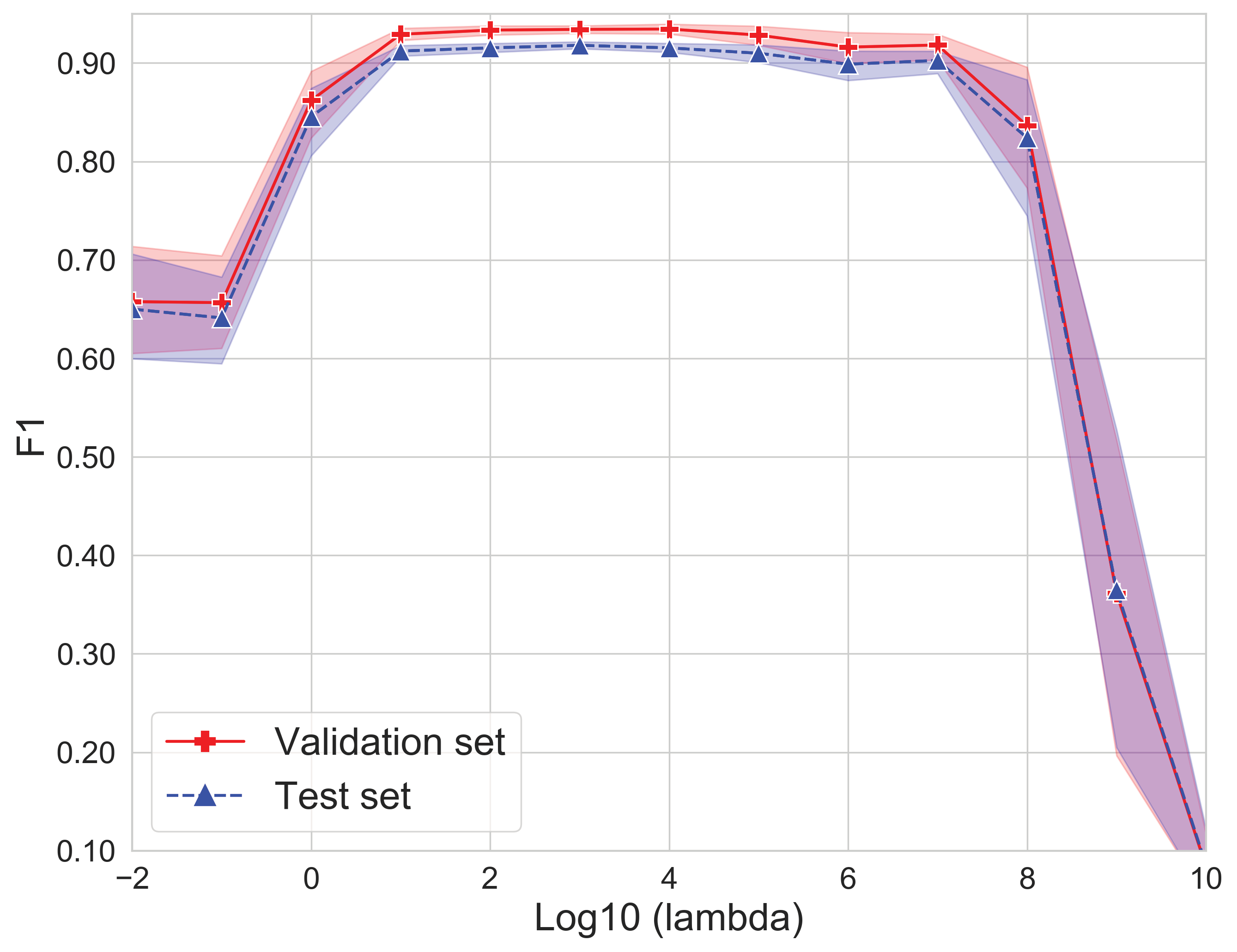
(a) AUC-2T performance

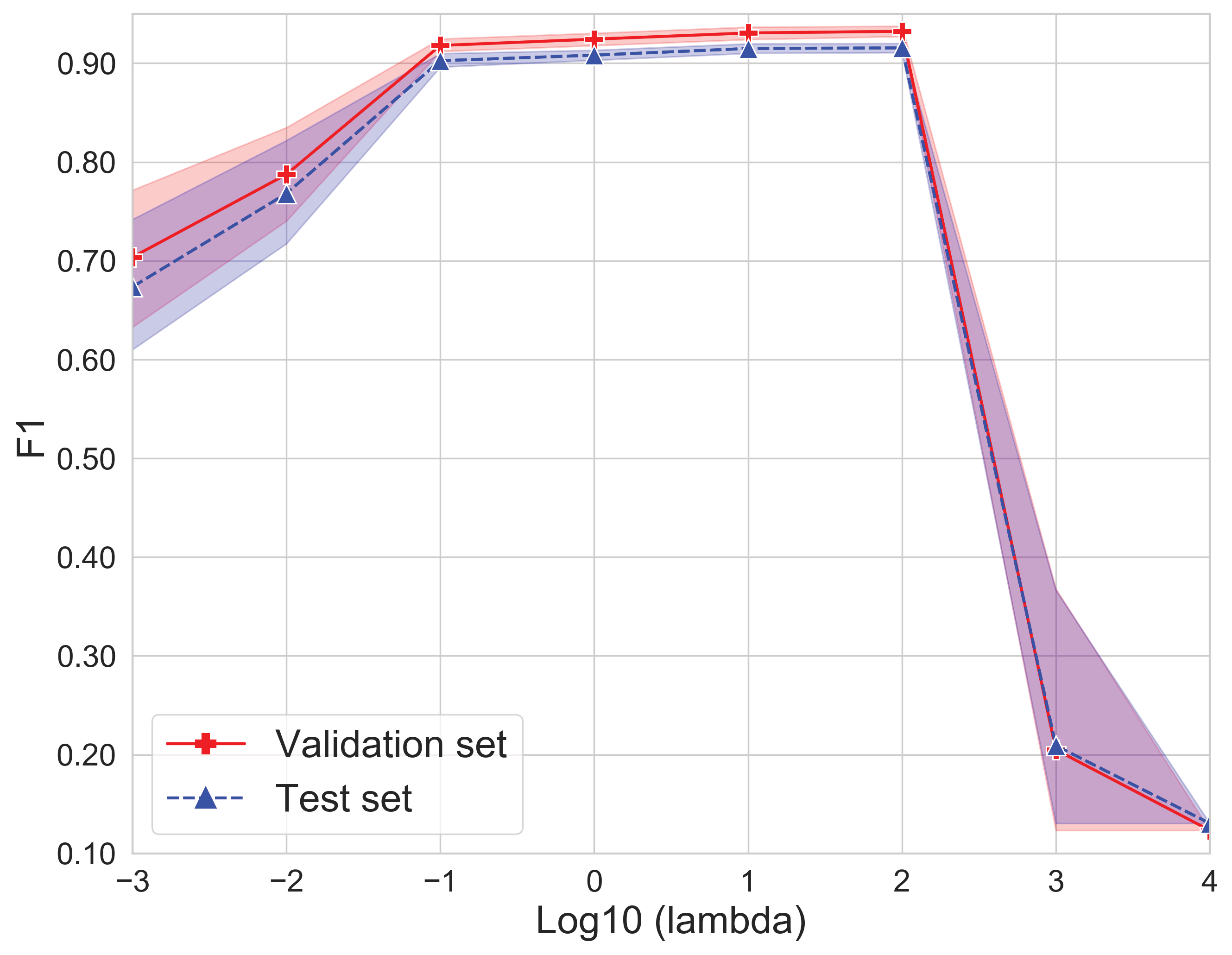
(b) COMAUC-2T performance

Figure 3: Average model performance taken from 10 random partitions of 200 CoNLL 2003 sentences. We plot F1-scores as a function of the logarithm of $\lambda$ values. In both plots, the red line represents the F1-scores based on the validation set and the blue dash line represents the F1-scores based on the test set. The error bands indicate the 95% confidence level of the F1-scores.

Model Architecture and Embedding

For embeddings and model architectures, we used both “bert-base-cased” (Devlin et al. 2019) and “facebook/bart-base” (Lewis et al. 2020) on CoNLL 2003 and OntoNotes5. “bert-base-cased” uses the transformers model architecture, while “facebook/bart-base” uses the seq2seq model architecture. By testing our AUC NER two-task method on different embeddings and model architectures, we give evidence that our method is also embedding and model agnostic. Due to their distinct linguistic characteristics which often lead to the out-of-vocabulary (OOV) issue when training with the standard language model embeddings, all biomedical corpora will be trained with “biobert-base-cased-v1.1” (Lee et al. 2019). The implementation of BioBERT, which achieved the state-of-the-art performance for many benchmark biomedical corpora, is publicly available at BioBERT github website (see https://github.com/dmis-lab/biobert (Lee et al. 2019)).

Low-Resource and Imbalanced Settings

To analyze the performance of our AUC NER two-task method under the low-resource and imbalanced distribution scenarios, we consider the following experimental settings:

• The size of training set $\mathcal{S}$: We used $\mathcal{S}$ with size $\in\{20,$ $50,100,150,200,250,300,350,400,450,500,1000\}$ to simulate the data scarcity issue in low-resource scenarios. Given the size of $\mathcal{S}$, we trained our method and all the baselines on multiple training partitions of the same size and report/investigate their average performance.

• We developed an imbalanced data generator for the NER task. This generator samples $\mathcal{S}$ that contains $\{1,2,5,10,20\}$ percentage of entity-tokens. By evaluating the performance of our method on different data distributions, we can indicate the robustness of our method under different imbalanced data distribution setups.

Baselines & AUC NER Two-Task Method

For our baselines, we chose the following methods:

• CE: The standard cross entropy loss, commonly used in NER, was used as one of the major baselines to verify the significance/impact of our method. We used all standard hyperparameter settings to record its performance.

• CRF: CRF represents our second major baseline as it has been traditionally used in many NER works, such as those of Huang, Xu, and Yu (2015); Lample et al. (2016); Xu et al. (2018, 2019). It should be noted that as CRF uses the transition matrix to generate the predictions, we cannot use the WordPiece tokenization for this baseline.

• CE-2T: This is our last baseline. For this baseline, we broke the standard multi-class NER setting into the two-task NER setting as shown in both Figure 1 and Figure 2. However, instead of optimizing both tasks under the AUC maximization approach, we used the binary cross entropy loss. This baseline serves to demonstrate that the significance of our work is related not only to the NER two-task setting but also to the AUC objective function.

For our AUC NER two-task method, we considered:

• AUC-2T: AUC-2T, one of the two implementations to verify the significance/impact of our work, learns the optimal $\mathbf{w}^{*}_{\textbf{en}}$, and $\mathbf{w}^{*}_{\textbf{be}}$ by minimizing Eq (4) during training.

• COMAUC-2T: COMAUC-2T also minimizes Eq (4) at training time. However, different from AUC-2T, COMAUC-2T learns $\mathbf{w}^{*}_{\textbf{en}}$ and $\mathbf{w}^{*}_{\textbf{be}}$ by following the idea proposed by Yuan et al. (2021a) and alternates between the standard multi-class cross entropy loss function and the AUC two-task loss function during training.

Both our AUC-2T and COMAUC-2T were set up for the NER task by modifying the code from libauc (Yuan et al. 2022). At prediction time, both AUC-2T and COMAUC-2T use Algorithm 1 to generate the BIO-tag for evaluation.

Evaluation Metrics

Since there is no agreed upon AUC evaluation metric for the NER task, we used the standard F1, precision and recall score to evaluate for all our setups (Nakayama 2018).

Experimental Results & Discussions

Training Size 20 50 100 Precision Recall F1 Precision Recall F1 Precision Recall F1 CE ${0.2889}_{0.0286}$ ${0.2425}_{0.0282}$ ${0.2189}_{0.0214}$ ${0.4451}_{0.0243}$ ${0.4011}_{0.0377}$ ${0.3921}_{0.0285}$ ${0.5953}_{0.0210}$ ${0.6683}_{0.0225}$ ${0.6253}_{0.0206}$ CRF ${0.5120}_{0.0156}$ ${0.5910}_{0.0228}$ ${0.5437}_{0.0177}$ ${0.6120}_{0.0125}$ ${0.6592}_{0.0129}$ ${0.6318}_{0.0108}$ ${0.6731}_{0.0150}$ ${0.6944}_{0.0122}$ ${0.6817}_{0.0124}$ CE-2T ${0.0783}_{0.0001}$ ${0.3915}_{0.0001}$ ${0.1304}_{0.0001}$ ${0.0783}_{0.0001}$ ${0.3915}_{0.0001}$ ${0.1304}_{0.0001}$ ${0.0783}_{0.0001}$ ${0.3915}_{0.0001}$ ${0.1304}_{0.0001}$ AUC-2T $\underline{0.5794}_{0.0264}$ $\underline{0.7000}_{0.0224}$ $\underline{0.6289}_{0.0241}$ $\underline{0.7976}_{0.0174}$ $\underline{0.8693}_{0.0076}$ $\underline{0.8300}_{0.0131}$ $\underline{0.8589}_{0.0139}$ $\underline{0.8973}_{0.0122}$ $\underline{0.8774}_{0.0131}$ COMAUC-2T ${\bf 0.6647}_{0.0257}$ ${\bf 0.7399}_{0.0225}$ ${\bf 0.6927}_{0.0220}$ ${\bf 0.8243}_{0.0191}$ ${\bf 0.8715}_{0.0106}$ ${\bf 0.8448}_{0.0149}$ ${\bf 0.8730}_{0.0108}$ ${\bf 0.9019}_{0.0103}$ ${\bf 0.8869}_{0.0102}$ Training Size 150 200 250 Precision Recall F1 Precision Recall F1 Precision Recall F1 CE ${0.7761}_{0.0188}$ ${0.8500}_{0.0110}$ ${0.8094}_{0.0159}$ ${0.8167}_{0.0149}$ ${0.8916}_{0.0043}$ ${0.8508}_{0.0103}$ ${0.8317}_{0.0168}$ ${0.9001}_{0.0037}$ ${0.8616}_{0.0117}$ CRF ${0.7056}_{0.0108}$ ${0.7187}_{0.0124}$ ${0.7099}_{0.0094}$ ${0.7165}_{0.0076}$ ${0.7254}_{0.0078}$ ${0.7196}_{0.0053}$ ${0.7293}_{0.0089}$ ${0.7437}_{0.0081}$ ${0.7351}_{0.0063}$ CE-2T ${0.0951}_{0.0167}$ ${0.3831}_{0.0082}$ ${0.1336}_{0.0031}$ ${0.3626}_{0.0565}$ ${0.4334}_{0.0186}$ ${0.3291}_{0.0411}$ ${0.3229}_{0.0553}$ ${0.4139}_{0.0179}$ ${0.2884}_{0.0384}$ AUC-2T $\underline{0.8718}_{0.0144}$ ${\bf 0.9150}_{0.0069}$ $\underline{0.8921}_{0.0110}$ $\underline{0.8827}_{0.0066}$ ${\bf 0.9180}_{0.0037}$ $\underline{0.8998}_{0.0048}$ $\underline{0.8875}_{0.0056}$ $\underline{0.9175}_{0.0058}$ $\underline{0.9020}_{0.0051}$ COMAUC-2T ${\bf 0.8814}_{0.0091}$ $\underline{0.9110}_{0.0094}$ ${\bf 0.8958}_{0.0091}$ ${\bf 0.8867}_{0.0062}$ $\underline{0.9170}_{0.0035}$ ${\bf 0.9014}_{0.0045}$ ${\bf 0.8943}_{0.0039}$ ${\bf 0.9198}_{0.0032}$ ${\bf 0.9068}_{0.0034}$ Training Size 300 350 400 Precision Recall F1 Precision Recall F1 Precision Recall F1 CE ${0.8503}_{0.0140}$ ${0.9110}_{0.0040}$ ${0.8778}_{0.0092}$ ${0.8763}_{0.0069}$ ${0.9192}_{0.0025}$ ${0.8969}_{0.0043}$ ${0.8880}_{0.0056}$ ${0.9229}_{0.0022}$ ${0.9049}_{0.0035}$ CRF ${0.7460}_{0.0093}$ ${0.7545}_{0.0070}$ ${0.7489}_{0.0061}$ ${0.7585}_{0.0073}$ ${0.7696}_{0.0056}$ ${0.7634}_{0.0053}$ ${0.7698}_{0.0058}$ ${0.7719}_{0.0063}$ ${0.7700}_{0.0040}$ CE-2T ${0.5172}_{0.0456}$ ${0.5512}_{0.0322}$ ${0.4990}_{0.0432}$ ${0.6043}_{0.0332}$ ${0.6695}_{0.0198}$ ${0.6250}_{0.0315}$ ${0.6298}_{0.0282}$ ${0.6937}_{0.0192}$ ${0.6529}_{0.0271}$ AUC-2T $\underline{0.8929}_{0.0084}$ $\underline{0.9185}_{0.0078}$ $\underline{0.9054}_{0.0081}$ ${\bf 0.9091}_{0.0024}$ $\underline{0.9283}_{0.0024}$ $\underline{0.9185}_{0.0020}$ $\underline{0.9081}_{0.0032}$ ${\bf 0.9324}_{0.0018}$ $\underline{0.9200}_{0.0019}$ COMAUC-2T ${\bf 0.9021}_{0.0032}$ ${\bf 0.9284}_{0.0027}$ ${\bf 0.9150}_{0.0026}$ $\underline{0.9081}_{0.0023}$ ${\bf 0.9298}_{0.0024}$ ${\bf 0.9188}_{0.0020}$ ${\bf 0.9092}_{0.0020}$ $\underline{0.9313}_{0.0024}$ ${\bf 0.9200}_{0.0018}$ Training Size 450 500 1000 Precision Recall F1 Precision Recall F1 Precision Recall F1 CE ${0.8926}_{0.0052}$ ${0.9268}_{0.0022}$ ${0.9092}_{0.0033}$ ${0.9009}_{0.0046}$ ${0.9292}_{0.0022}$ ${0.9147}_{0.0031}$ $\underline{0.9294}_{0.0015}$ ${\bf 0.9480}_{0.0013}$ ${\bf 0.9386}_{0.0011}$ CRF ${0.7673}_{0.0050}$ ${0.7759}_{0.0084}$ ${0.7705}_{0.0046}$ ${0.7880}_{0.0048}$ ${0.7834}_{0.0081}$ ${0.7849}_{0.0050}$ ${0.8336}_{0.0053}$ ${0.8402}_{0.0052}$ ${0.8365}_{0.0042}$ CE-2T ${0.6633}_{0.0093}$ ${0.7275}_{0.0107}$ ${0.6928}_{0.0090}$ ${0.6685}_{0.0077}$ ${0.7386}_{0.0089}$ ${0.7007}_{0.0070}$ ${0.7552}_{0.0071}$ ${0.8648}_{0.0066}$ ${0.8060}_{0.0066}$ AUC-2T ${\bf 0.9087}_{0.0033}$ $\underline{0.9311}_{0.0026}$ $\underline{0.9197}_{0.0023}$ ${\bf 0.9141}_{0.0023}$ $\underline{0.9333}_{0.0024}$ ${\bf 0.9235}_{0.0018}$ ${0.9254}_{0.0014}$ ${0.9450}_{0.0010}$ ${0.9351}_{0.0009}$ COMAUC-2T $\underline{0.9086}_{0.0023}$ ${\bf 0.9318}_{0.0020}$ ${\bf 0.9200}_{0.0017}$ $\underline{0.9122}_{0.0025}$ ${\bf 0.9343}_{0.0023}$ $\underline{0.9231}_{0.0019}$ ${\bf 0.9303}_{0.0015}$ $\underline{0.9458}_{0.0010}$ $\underline{0.9379}_{0.0009}$

Table 2: Average performance taken from 30 random partitions of different training set sizes. The non-parametric bootstrapped standard errors from these experiments are under-scripted. The best performance for each setting is bold while the second best is underlined. The model architecture is “transformers” and the token embeddings is “bert-base-cased” (Devlin et al. 2019).

Ablation Studies

Under our AUC NER two-task setups, the hyperparameter $\lambda$ controls the trade-off between the two tasks (see Eq (4)). Our intuitions tell us that $\lambda\gg 1$ since being in an NE is the dominant factor and unless 2 NEs run together, it is all that is needed. We admit that choosing a good $\lambda$ for both AUC-2T and COMAUC-2T could be adhoc. Thus, we greedily searched for the optimal $\lambda$ by training both setups multiple times with different partitions of 200 sentences and record their performance for different $\lambda$ values. The results are presented in Figure 3 and the optimums are wide and flat. Both Figure 3(a) and Figure 3(b) suggest that AUC-2T and COMAUC-2T reach their optimal performance at $\lambda=100$. Since the beginning-token prediction task is more imbalanced than the entity-token prediction task, we believe that $\lambda=100$ is large enough so that the gradients from $\text{AUC}_{\mathrm{M}}(\mathbf{w}_{\textbf{be}})$ is sufficiently represented when Eq (4) is optimized. For the rest of the paper, we present the results for AUC-2T and COMAUC-2T with $\lambda=100$ during training.

Low-Resource Studies

Figure 4: Learning curves of the average performance taken from 10 random data partitions, each partition with the size of 100 sentences (i.e., $\approx$ 1,211 tokens). The original BIO label distribution for CoNLL 2003 is $11.5\%$, $5.2\%$, and $83.3\%$ respectively (see Table 1), i.e., original entity label size $=16.7\%$. The entity label size in this graph represents the percentage of entity-tokens over the number of tokens for the training set $\mathcal{S}$. The error bands indicate the $95\%$ confidence level of the scores.

Using the results from both Table 2 in this section and Figure 5 in the appendix, we have the following observations:

• CE vs. AUC-2T: Under the extreme low-resource settings (i.e., size of $\{20,50\}$), AUC-2T outperforms CE with a noticeable margin, with the average difference in the F1-performance getting as big as $40\%$. When the training set size gets bigger, AUC-2T still shows improvements compared to CE, most of the times with significant improvements at the 95% level of confidence. When the training set size is $1000$, CE outperforms AUC-2T on average; however, we argue that this is not significant and the difference is negligible. Furthermore, except for the training set size of $20$, AUC-2T outputs more stable results compared to CE as indicated by their standard errors. This comparison gives evidence that AUC-2T is a better objective function for the low-resource NER settings compared to the standard CE objective function.

• CRF vs. AUC-2T: Albeit losing significantly across the performance metrics to AUC-2T under all settings, CRF still produces quite stable results in some cases. Nonetheless, given the results, we believe that AUC-2T is a better alternative to CRF under the low-resource NER settings.

• CE-2T vs. AUC-2T: CE-2T is our last and weakest baseline; thus, it is not surprising that it performs the worst. This happens since while AUC-2T puts equal focus on both positive and negative-class tokens, CE, due to its nature of following the maximum likelihood principle, tends to favor the class with the majority presence during training. Although they should give similar results asymptotically, it is clear that all CE objective/loss functions suffer when the data is inherently imbalanced, as is the case of the NER task. Since we reformulate the original multi-class setting into the two-task setting, this amplifies the imbalanced data distribution issue, at least for the beginning-token prediction task. Thus, it is unsurprising that CE-2T gives poor performance and only recovers/improves when the size of $\mathcal{S}$ gets bigger. Comparing CE-2T with AUC-2T reveals that maximizing AUC scores contributes substantially to the NER performance.

• COMAUC-2T vs. AUC-2T: Although the F1-score of COMAUC-2T is higher on average than that of AUC-2T under almost all settings, the difference between the two approaches is not significant, particularly when the size of $\mathcal{S}$ is large. Since COMAUC-2T alternates between the standard multi-class cross entropy loss function and the AUC two-task loss function during training, we surmise the difference is due to 1) better learned feature representations (i.e., embeddings, transformers) from minimizing the standard CE loss function as theoretically proven by Yuan et al. (2021a), and 2) higher training time complexity as COMAUC-2T time complexity $=$ AUC-2T time complexity $+$ CE time complexity. Since COMAUC-2T performs on par with AUC-2T, it consequently outperforms all baselines in most low-resource NER settings.

We can observe similar result patterns to those mentioned above in the sub-section “low-resource studies” found in the supplementary material. These results are collected from different data domains (general, disease, species), embeddings (bert-base-cased, facebook/bart-base, biobert-base-cased-v1.1), and model architectures (transformers, seq2seq). Consequently, they strengthen the evidence that our method is domain, embedding, and model agnostic.

Predicting PER (5.4% of tokens) as the entity type

Training Size 50 100 200 Precision Recall F1 Precision Recall F1 Precision Recall F1 DL ${0.0177}_{0.0021}$ ${0.0062}_{0.0006}$ ${0.0089}_{0.0008}$ ${0.0188}_{0.0014}$ ${0.0070}_{0.0005}$ ${0.0101}_{0.0007}$ ${0.0219}_{0.0022}$ ${0.0068}_{0.0010}$ ${0.0102}_{0.0012}$ AUC-2T ${\bf 0.8102}_{0.0161}$ ${\bf 0.8199}_{0.0274}$ ${\bf 0.8131}_{0.0188}$ $\underline{0.8640}_{0.0086}$ ${\bf 0.8975}_{0.0112}$ ${\bf 0.8796}_{0.0058}$ ${\bf 0.8824}_{0.0109}$ $\underline{0.8955}_{0.0090}$ $\underline{0.8884}_{0.0076}$ COMAUC-2T $\underline{0.8037}_{0.0153}$ $\underline{0.8134}_{0.0253}$ $\underline{0.8068}_{0.0175}$ ${\bf 0.8786}_{0.0117}$ $\underline{0.8461}_{0.0170}$ $\underline{0.8606}_{0.0095}$ $\underline{0.8727}_{0.0059}$ ${\bf 0.9067}_{0.0104}$ ${\bf 0.8890}_{0.0060}$ Training Size 400 500 1000 Precision Recall F1 Precision Recall F1 Precision Recall F1 DL ${0.0636}_{0.0062}$ ${0.0154}_{0.0012}$ ${0.0246}_{0.0019}$ ${0.1859}_{0.0101}$ ${0.0421}_{0.0025}$ ${0.0677}_{0.0033}$ ${0.7893}_{0.0105}$ ${0.5505}_{0.0082}$ ${0.6486}_{0.0090}$ AUC-2T $\underline{0.9021}_{0.0054}$ ${\bf 0.9144}_{0.0086}$ $\underline{0.9078}_{0.0043}$ ${\bf 0.9140}_{0.0074}$ ${\bf 0.9249}_{0.0073}$ ${\bf 0.9191}_{0.0054}$ $\underline{0.9181}_{0.0057}$ ${\bf 0.9354}_{0.0032}$ $\underline{0.9266}_{0.0039}$ COMAUC-2T ${\bf 0.9094}_{0.0044}$ $\underline{0.9116}_{0.0045}$ ${\bf 0.9105}_{0.0038}$ $\underline{0.9115}_{0.0064}$ $\underline{0.9213}_{0.0081}$ $\underline{0.9162}_{0.0061}$ ${\bf 0.9296}_{0.0064}$ $\underline{0.9341}_{0.0046}$ ${\bf 0.9317}_{0.0039}$

Predicting LOC (4.1% of tokens) as the entity type

Training Size 50 100 200 Precision Recall F1 Precision Recall F1 Precision Recall F1 DL ${0.0460}_{0.0041}$ ${0.0229}_{0.0018}$ ${0.0297}_{0.0021}$ ${0.0332}_{0.0030}$ ${0.0178}_{0.0012}$ ${0.0226}_{0.0013}$ ${0.0349}_{0.0035}$ ${0.0176}_{0.0008}$ ${0.0230}_{0.0013}$ AUC-2T $\underline{0.5225}_{0.0195}$ $\underline{0.6674}_{0.0436}$ $\underline{0.5779}_{0.0241}$ $\underline{0.6203}_{0.0273}$ ${\bf 0.6959}_{0.0232}$ $\underline{0.6512}_{0.0182}$ $\underline{0.6547}_{0.0293}$ ${\bf 0.8153}_{0.0149}$ $\underline{0.7205}_{0.0148}$ COMAUC-2T ${\bf 0.5828}_{0.0311}$ ${\bf 0.6766}_{0.0334}$ ${\bf 0.6180}_{0.0218}$ ${\bf 0.6468}_{0.0262}$ $\underline{0.6886}_{0.0300}$ $\underline{0.6629}_{0.0218}$ ${\bf 0.7044}_{0.0273}$ $\underline{0.7784}_{0.0159}$ ${\bf 0.7341}_{0.0125}$ Training Size 400 500 1000 Precision Recall F1 Precision Recall F1 Precision Recall F1 DL ${0.0469}_{0.0068}$ ${0.0224}_{0.0017}$ ${0.0288}_{0.0024}$ ${0.1209}_{0.0204}$ ${0.0282}_{0.0025}$ ${0.0451}_{0.0045}$ ${0.5953}_{0.0142}$ ${0.5656}_{0.0162}$ ${0.5766}_{0.0064}$ AUC-2T ${\bf 0.7594}_{0.0180}$ ${\bf 0.8306}_{0.0467}$ ${\bf 0.7908}_{0.0084}$ ${\bf 0.7737}_{0.0163}$ ${\bf 0.8269}_{0.0132}$ ${\bf 0.7979}_{0.0108}$ $\underline{0.8291}_{0.0172}$ ${\bf 0.8818}_{0.0169}$ $\underline{0.8538}_{0.0103}$ COMAUC-2T $\underline{0.7492}_{0.0224}$ $\underline{0.8267}_{0.0076}$ $\underline{0.7835}_{0.0114}$ $\underline{0.7641}_{0.0178}$ $\underline{0.8220}_{0.0082}$ $\underline{0.7910}_{0.0118}$ ${\bf 0.8467}_{0.0180}$ $\underline{0.8706}_{0.0059}$ ${\bf 0.8573}_{0.0100}$

Predicting ORG (4.9% of tokens) as the entity type

Training Size 50 100 200 Precision Recall F1 Precision Recall F1 Precision Recall F1 DL ${0.0394}_{0.0108}$ ${0.0056}_{0.0011}$ ${0.0093}_{0.0020}$ ${0.0113}_{0.0025}$ ${0.0047}_{0.0004}$ ${0.0061}_{0.0005}$ ${0.0103}_{0.0044}$ ${0.0064}_{0.0020}$ ${0.0056}_{0.0018}$ AUC-2T ${\bf 0.4536}_{0.0377}$ ${\bf 0.3155}_{0.0471}$ ${\bf 0.3401}_{0.0320}$ ${\bf 0.4720}_{0.0288}$ ${\bf 0.4250}_{0.0572}$ ${\bf 0.4288}_{0.0401}$ ${\bf 0.6147}_{0.0262}$ ${\bf 0.5128}_{0.0248}$ ${\bf 0.5566}_{0.0227}$ COMAUC-2T $\underline{0.3921}_{0.0253}$ $\underline{0.2906}_{0.0459}$ $\underline{0.3113}_{0.0336}$ $\underline{0.4509}_{0.0334}$ $\underline{0.3764}_{0.0514}$ $\underline{0.3907}_{0.0385}$ $\underline{0.5982}_{0.0181}$ $\underline{0.4845}_{0.0249}$ $\underline{0.5312}_{0.0190}$ Training Size 400 500 1000 Precision Recall F1 Precision Recall F1 Precision Recall F1 DL ${0.0031}_{0.0005}$ ${0.0034}_{0.0008}$ ${0.0026}_{0.0002}$ ${0.0117}_{0.0038}$ ${0.0033}_{0.0009}$ ${0.0044}_{0.0012}$ ${0.3212}_{0.0381}$ ${0.2059}_{0.0265}$ ${0.2236}_{0.0242}$ AUC-2T $\underline{0.6799}_{0.0255}$ ${\bf 0.6265}_{0.0386}$ ${\bf 0.6469}_{0.0292}$ $\underline{0.6959}_{0.0134}$ ${\bf 0.6518}_{0.0344}$ ${\bf 0.6671}_{0.0208}$ $\underline{0.7608}_{0.0160}$ $\underline{0.7498}_{0.0322}$ $\underline{0.7533}_{0.0240}$ COMAUC-2T ${\bf 0.6906}_{0.0186}$ $\underline{0.6105}_{0.0368}$ $\underline{0.6442}_{0.0259}$ ${\bf 0.7129}_{0.0135}$ $\underline{0.6217}_{0.0358}$ $\underline{0.6552}_{0.0223}$ ${\bf 0.7669}_{0.0185}$ ${\bf 0.7601}_{0.0303}$ ${\bf 0.7612}_{0.0220}$

Predicting MISC (2.3% of tokens) as the entity type

Training Size 50 100 200 Precision Recall F1 Precision Recall F1 Precision Recall F1 DL ${0.0021}_{0.0010}$ ${0.0013}_{0.0005}$ ${0.0010}_{0.0003}$ ${0.0018}_{0.0004}$ ${0.0038}_{0.0013}$ ${0.0017}_{0.0002}$ ${0.0033}_{0.0011}$ ${0.0031}_{0.0007}$ ${0.0027}_{0.0006}$ AUC-2T $\underline{0.4257}_{0.0776}$ $\underline{0.2969}_{0.0503}$ $\underline{0.3292}_{0.0572}$ $\underline{0.4234}_{0.0746}$ $\underline{0.3718}_{0.0439}$ $\underline{0.3816}_{0.0527}$ $\underline{0.5638}_{0.0436}$ ${\bf 0.5456}_{0.0319}$ ${\bf 0.5486}_{0.0318}$ COMAUC-2T ${\bf 0.4710}_{0.0771}$ ${\bf 0.3311}_{0.0438}$ ${\bf 0.3805}_{0.0550}$ ${\bf 0.4351}_{0.0714}$ ${\bf 0.3772}_{0.0437}$ ${\bf 0.3941}_{0.0522}$ ${\bf 0.5707}_{0.0499}$ $\underline{0.5395}_{0.0271}$ $\underline{0.5462}_{0.0355}$ Training Size 400 500 1000 Precision Recall F1 Precision Recall F1 Precision Recall F1 DL ${0.0007}_{0.0001}$ ${0.0059}_{0.0016}$ ${0.0011}_{0.0001}$ ${0.0009}_{0.0001}$ ${0.0064}_{0.0015}$ ${0.0014}_{0.0001}$ ${0.0007}_{0.0001}$ ${0.0118}_{0.0001}$ ${0.0014}_{0.0001}$ AUC-2T $\underline{0.6341}_{0.0304}$ ${\bf 0.6060}_{0.027}$ $\underline{0.6184}_{0.0269}$ $\underline{0.6468}_{0.0294}$ $\underline{0.6091}_{0.0306}$ $\underline{0.6260}_{0.0289}$ ${\bf 0.7385}_{0.0110}$ $\underline{0.6830}_{0.0088}$ ${\bf 0.7091}_{0.0075}$ COMAUC-2T ${\bf 0.6525}_{0.0268}$ $\underline{0.6047}_{0.0177}$ ${\bf 0.6264}_{0.0203}$ ${\bf 0.6744}_{0.0316}$ ${\bf 0.6155}_{0.0232}$ ${\bf 0.6426}_{0.0264}$ $\underline{0.7308}_{0.0118}$ ${\bf 0.6869}_{0.0082}$ $\underline{0.7073}_{0.0064}$

Table 3: Average performance taken from 10 random partitions of different training set sizes. The non-parametric bootstrapped standard errors from these experiments are under-scripted. The best performance for each setting is bold while the second best is underlined. The model architecture is “transformers” and the token embeddings is “bert-base-cased” (Devlin et al. 2019).

Imbalanced Data Distribution Studies

As previously mentioned, we developed an imbalanced data generator for the NER task. This generator serves to simulate the scenarios where the data distribution for $\mathcal{S}$ is different from that of $\mathcal{S}_{\text{test}}$, testing the robustness of both the baselines and our method. We present the main result in Figure 4. From this result, we have the following observations:

• CE vs. AUC-2T: We found that with the extreme imbalanced training sets (i.e., entity label size of $1$ and $2\%$), CE performs extremely poorly even when the training size is reasonably adequate. The F1-score drops even lower than training with 20 sentences as indicated in Table 2. Although the F1-score for AUC-2T also dropped given these settings, the drop is not as significant as CE. Additionally, we observe that the performance of AUC-2T under these extreme settings is still on par with that of CE when training with the normal training set $\mathcal{S}$ (Table 2).

• CRF vs. AUC-2T: Although CRF performance drops under the extreme imbalanced settings, the decline is not as severe as that of CE, showing the robustness of CRF loss function. Additionally, both AUC-2T and CRF improve with more entities in $\mathcal{S}$ at a similar rate. However, as AUC excels under the imbalanced settings, the performance gap between AUC-2T and CRF is still significant.

• COMAUC-2T vs. AUC-2T: Both approaches show similar F1-performance across different entity label size. As AUC-2T has shown its robustness compared to other loss/objective functions, COMAUC-2T consequently can be considered as a better alternative to its baselines.

• Lastly, the results also indicate that having more NEs in $\mathcal{S}$ will lead to higher F1-scores on $\mathcal{S}_{\text{test}}$ for all approaches, regardless of the data distribution differences between $\mathcal{S}$ and $\mathcal{S}_{\text{test}}$. We surmise this happens as more NEs means more information for training the model parameters. This is consistent with the results from Nguyen et al. (2022).

Note that we excluded CE-2T from our results and discussions as it already exhibits poor performance under the standard imbalance setting. We also provide experimental results for different training-set sizes, domains, embeddings, and model architectures in sub-section “imbalanced data distribution studies” in the supplementary material. From these results, we can observe similar result patterns with those in Figure 4, indicating the robustness of our approach.

Comparison with Other NER Imbalanced Losses

Lastly, we compare our low-resource NER solutions to Dice Loss (Li et al. 2020), which is based on the Sørensen–Dice coefficient (Sorensen 1948) to alleviate the influences of negative examples in the NER problem. The corpus we used for our experiments is CoNLL 2003 as it is the corpus used by Li et al. (2020) in their paper to present the findings. As Dice Loss (DL) attempts to find both the entity tokens and their entity type, we modify the original codes  so that both our methods and Dice Loss only focus on a specific entity type, say LOC, i.e., we train the model to predict the BIO tag for only the LOC tokens. Please note that since we only predict for the a single type of entities (e.g., LOC), the percentage of entity tokens is drastically lower than 16.7% (see Table 1) , making the distribution more imbalanced and the problem harder to solve. We present the experimental results in Table 3 and provide the following observations:

• AUC-2T vs. COMAUC-2T: Our two methods still exhibit consistently strong performance under this new experimental setting. The difference in term of performance (precision, recall and f1) between the two methods, with a 95% confident level, are not significant under all cases, which aligns with our findings from previous sections.

• AUC-2T vs. DL: Under the low-resource settings, our AUC-2T outperforms Dice Loss significantly. We presume this happens since while Dice Loss shows great performance when all training data are available (Li et al. 2020), the low-resource settings exacerbate the challenge of the NER tasks. For entity type that appears sparingly in the corpus (e.g., MISC), Dice Loss struggles even with 1000 training sentences as there is little learning signals for its algorithm to work with. Although Dice Loss demonstrates great improvement for some entity types once the training pool is large enough, we believe that both of our methods should be the preferred alternative under the low-resource NER settings. As AUC-2T outperforms Dice Loss significantly, our COMAUC-2T also displays a strong performance against Dice Loss.

Conclusions

In this paper, we studied an effective solution to the low-resource and the data imbalance issues that widely exist in many NER/BioNER tasks. To tackle these two issues, we have first reformulated the conventional NER task as a two-task learning problem, which consists of two binary classifiers predicting if a word is a part of an NE and if the word is the start of an NE respectively. We then adapted the idea of AUC maximization to develop a new NER loss based on the reformulation. Extensive experiments on different datasets with different scenarios, which mimic the low-resource and the data imbalance issues, demonstrated that the new AUC-based loss function performs substantially better than the commonly used CE and CRF, regardless of the underlying NER models, embeddings or domains that we used. Although the proposed AUC optimization approach works quite well for NER, there still exist some limitations, including the inconsistency in the prediction that arises from the two-task reformulation of NER. We believe that the AUC optimization for the multi-class problem (Yang et al. 2021) could be an alternative, which is subject to future work.

References

- Banerjee et al. (2019) Banerjee, P. S.; Chakraborty, B.; Tripathi, D.; Gupta, H.; and Kumar, S. S. 2019. A information retrieval based on question and answering and NER for unstructured information without using SQL. Wireless Personal Communications, 108(3): 1909–1931.
- Chen et al. (2021) Chen, S.; Aguilar, G.; Neves, L.; and Solorio, T. 2021. Data Augmentation for Cross-Domain Named Entity Recognition. In Proceedings of the 2021 Conference on Empirical Methods in Natural Language Processing, 5346–5356. Online and Punta Cana, Dominican Republic: Association for Computational Linguistics.
- Clémençon, Lugosi, and Vayatis (2008) Clémençon, S.; Lugosi, G.; and Vayatis, N. 2008. Ranking and empirical minimization of U-statistics. The Annals of Statistics, 36(2): 844–874.
- Devlin et al. (2019) Devlin, J.; Chang, M.-W.; Lee, K.; and Toutanova, K. 2019. BERT: Pre-training of Deep Bidirectional Transformers for Language Understanding. In Proceedings of the 2019 Conference of the North American Chapter of the Association for Computational Linguistics: Human Language Technologies, Volume 1 (Long and Short Papers), 4171–4186. Minneapolis, Minnesota: Association for Computational Linguistics.
- Doğan, Leaman, and Lu (2014) Doğan, R. I.; Leaman, R.; and Lu, Z. 2014. Special Report: NCBI Disease Corpus: A Resource for Disease Name Recognition and Concept Normalization. J. of Biomedical Informatics, 47: 1–10.
- Etzioni et al. (2005) Etzioni, O.; Cafarella, M.; Downey, D.; Popescu, A.-M.; Shaked, T.; Soderland, S.; Weld, D. S.; and Yates, A. 2005. Unsupervised named-entity extraction from the web: An experimental study. Artificial intelligence, 165(1): 91–134.
- Freund et al. (2003) Freund, Y.; Iyer, R.; Schapire, R. E.; and Singer, Y. 2003. An efficient boosting algorithm for combining preferences. Journal of machine learning research, 4(Nov): 933–969.
- Gao et al. (2013) Gao, W.; Jin, R.; Zhu, S.; and Zhou, Z.-H. 2013. One-pass AUC optimization. In International conference on machine learning, 906–914. PMLR.
- Gerner, Nenadic, and Bergman (2010) Gerner, M.; Nenadic, G.; and Bergman, C. 2010. LINNAEUS: A species name identification system for biomedical literature. BMC bioinformatics, 11: 85.
- Giorgi and Bader (2019) Giorgi, J. M.; and Bader, G. D. 2019. Towards reliable named entity recognition in the biomedical domain. Bioinformatics, 36(1): 280–286.
- Hanley and McNeil (1982) Hanley, J. A.; and McNeil, B. J. 1982. The meaning and use of the area under a receiver operating characteristic (ROC) curve. Radiology, 143(1): 29–36.
- Huang, Xu, and Yu (2015) Huang, Z.; Xu, W.; and Yu, K. 2015. Bidirectional LSTM-CRF Models for Sequence Tagging. arXiv:1508.01991.
- Kotlowski, Dembczynski, and Huellermeier (2011) Kotlowski, W.; Dembczynski, K.; and Huellermeier, E. 2011. Bipartite ranking through minimization of univariate loss. In ICML.
- Kripke (1980) Kripke, S. 1980. Naming and Necessity. Harvard University Press.
- Lample et al. (2016) Lample, G.; Ballesteros, M.; Subramanian, S.; Kawakami, K.; and Dyer, C. 2016. Neural Architectures for Named Entity Recognition. In Proceedings of the 2016 Conference of the North American Chapter of the Association for Computational Linguistics: Human Language Technologies, 260–270. San Diego, California: Association for Computational Linguistics.
- Lee et al. (2019) Lee, J.; Yoon, W.; Kim, S.; Kim, D.; Kim, S.; So, C. H.; and Kang, J. 2019. BioBERT: a pre-trained biomedical language representation model for biomedical text mining. Bioinformatics, 36(4): 1234–1240.
- Lewis et al. (2020) Lewis, M.; Liu, Y.; Goyal, N.; Ghazvininejad, M.; Mohamed, A.; Levy, O.; Stoyanov, V.; and Zettlemoyer, L. 2020. BART: Denoising Sequence-to-Sequence Pre-training for Natural Language Generation, Translation, and Comprehension. In Proceedings of the 58th Annual Meeting of the Association for Computational Linguistics, 7871–7880. Online: Association for Computational Linguistics.
- Li, Shang, and Shao (2020) Li, J.; Shang, S.; and Shao, L. 2020. MetaNER: Named Entity Recognition with Meta-Learning. In Proceedings of The Web Conference 2020, WWW ’20, 429–440. New York, NY, USA: Association for Computing Machinery. ISBN 9781450370233.
- Li et al. (2020) Li, J.; Sun, A.; Han, J.; and Li, C. 2020. A Survey on Deep Learning for Named Entity Recognition. IEEE Transactions on Knowledge and Data Engineering, 1–1.
- Li et al. (2020) Li, X.; Sun, X.; Meng, Y.; Liang, J.; Wu, F.; and Li, J. 2020. Dice Loss for Data-imbalanced NLP Tasks. In Proceedings of the 58th Annual Meeting of the Association for Computational Linguistics, 465–476. Online: Association for Computational Linguistics.
- Liu et al. (2020) Liu, M.; Yuan, Z.; Ying, Y.; and Yang, T. 2020. Stochastic AUC Maximization with Deep Neural Networks. In International Conference on Learning Representations.
- Liu et al. (2018) Liu, M.; Zhang, X.; Chen, Z.; Wang, X.; and Yang, T. 2018. Fast stochastic AUC maximization with -convergence rate. In International Conference on Machine Learning, 3189–3197. PMLR.
- Nakayama (2018) Nakayama, H. 2018. seqeval: A Python framework for sequence labeling evaluation. https://github.com/chakki-works/seqeval. Accessed: 2022-07-15.
- Natole, Ying, and Lyu (2018) Natole, M.; Ying, Y.; and Lyu, S. 2018. Stochastic proximal algorithms for AUC maximization. In International Conference on Machine Learning, 3710–3719. PMLR.
- Nguyen et al. (2022) Nguyen, N. D.; Du, L.; Buntine, W.; Chen, C.; and Beare, R. 2022. Hardness-guided domain adaptation to recognise biomedical named entities under low-resource scenarios. In Proceedings of the 2022 Conference on Empirical Methods in Natural Language Processing, 4063–4071. Abu Dhabi, United Arab Emirates: Association for Computational Linguistics.
- Pafilis et al. (2013) Pafilis, E.; Frankild, S. P.; Fanini, L.; Faulwetter, S.; Pavloudi, C.; Vasileiadou, A.; Arvanitidis, C.; and Jensen, L. J. 2013. The SPECIES and ORGANISMS Resources for Fast and Accurate Identification of Taxonomic Names in Text. PLOS ONE, 8(6): 1–6.
- Patel et al. (2005) Patel, V. L.; Patel, N.; Arocha, J. F.; and Zhang, J. 2005. Thinking and Reasoning in Medicine. The Cambridge handbook of thinking and reasoning, 14: 727–750.
- Peng et al. (2021) Peng, B.; Li, C.; Li, J.; Shayandeh, S.; Liden, L.; and Gao, J. 2021. Soloist: Building Task Bots at Scale with Transfer Learning and Machine Teaching. Transactions of the Association for Computational Linguistics, 9: 807–824.
- Rahimi, Li, and Cohn (2019) Rahimi, A.; Li, Y.; and Cohn, T. 2019. Massively Multilingual Transfer for NER. In Proceedings of the 57th Annual Meeting of the Association for Computational Linguistics, 151–164. Florence, Italy: Association for Computational Linguistics.
- Ritter, Etzioni, and Clark (2012) Ritter, A.; Etzioni, O.; and Clark, S. 2012. Open domain event extraction from Twitter. In Proceedings of the 18th ACM SIGKDD international conference on Knowledge discovery and data mining, 1104–1112.
- Sorensen (1948) Sorensen, T. A. 1948. A method of establishing groups of equal amplitude in plant sociology based on similarity of species content and its application to analyses of the vegetation on Danish commons. Biol. Skar., 5: 1–34.
- Tan, Du, and Buntine (2021) Tan, W.; Du, L.; and Buntine, W. 2021. Diversity Enhanced Active Learning with Strictly Proper Scoring Rules. In Ranzato, M.; Beygelzimer, A.; Dauphin, Y.; Liang, P.; and Vaughan, J. W., eds., Advances in Neural Information Processing Systems, volume 34, 10906–10918. Curran Associates, Inc.
- Tjong Kim Sang and De Meulder (2003) Tjong Kim Sang, E. F.; and De Meulder, F. 2003. Introduction to the CoNLL-2003 Shared Task: Language-Independent Named Entity Recognition. In Proceedings of the Seventh Conference on Natural Language Learning at HLT-NAACL 2003, 142–147.
- Weischedel et al. (2014) Weischedel, R.; Pradhan, S.; Ramshaw, L.; Palmer, M.; Xue, N.; Marcus, M.; Taylor, A.; Greenberg, C.; Hovy, E.; Belvin, R.; et al. 2014. Ontonotes release 5.0. LDC2011T03, Philadelphia, Penn.: Linguistic Data Consortium.
- Xu et al. (2019) Xu, K.; Yang, Z.; Kang, P.; Wang, Q.; and Liu, W. 2019. Document-level attention-based BiLSTM-CRF incorporating disease dictionary for disease named entity recognition. Computers in Biology and Medicine, 108: 122 – 132.
- Xu et al. (2018) Xu, K.; Zhou, Z.; Hao, T.; and Liu, W. 2018. A Bidirectional LSTM and Conditional Random Fields Approach to Medical Named Entity Recognition. In Hassanien, A. E.; Shaalan, K.; Gaber, T.; and Tolba, M. F., eds., Proceedings of the International Conference on Advanced Intelligent Systems and Informatics 2017, 355–365. Cham: Springer International Publishing. ISBN 978-3-319-64861-3.
- Yadav and Bethard (2018) Yadav, V.; and Bethard, S. 2018. A Survey on Recent Advances in Named Entity Recognition from Deep Learning models. In Proceedings of the 27th International Conference on Computational Linguistics, 2145–2158. Santa Fe, New Mexico, USA: Association for Computational Linguistics.
- Yang et al. (2021) Yang, Z.; Xu, Q.; Bao, S.; Cao, X.; and Huang, Q. 2021. Learning with Multiclass AUC: Theory and Algorithms. IEEE Transactions on Pattern Analysis and Machine Intelligence.
- Ying, Wen, and Lyu (2016) Ying, Y.; Wen, L.; and Lyu, S. 2016. Stochastic online auc maximization. Advances in neural information processing systems, 29.
- Yuan et al. (2021a) Yuan, Z.; Guo, Z.; Chawla, N.; and Yang, T. 2021a. Compositional Training for End-to-End Deep AUC Maximization. In International Conference on Learning Representations.
- Yuan et al. (2022) Yuan, Z.; Qiu, Z.-H.; Li, G.; Zhu, D.; Guo, Z.; Hu, Q.; Wang, B.; Qi, Q.; Zhong, Y.; and Yang, T. 2022. LibAUC: A Deep Learning Library for X-risk Optimization. https://https://libauc.org/. Accessed: 2022-07-11.
- Yuan et al. (2021b) Yuan, Z.; Yan, Y.; Sonka, M.; and Yang, T. 2021b. Large-scale Robust Deep AUC Maximization: A New Surrogate Loss and Empirical Studies on Medical Image Classification. In 2021 IEEE/CVF International Conference on Computer Vision (ICCV), 3020–3029. Los Alamitos, CA, USA: IEEE Computer Society.
- Zhao et al. (2011) Zhao, P.; Hoi, S. C. H.; Jin, R.; and Yang, T. 2011. Online AUC Maximization. In Proceedings of the 28th International Conference on International Conference on Machine Learning, ICML’11, 233–240. Madison, WI, USA: Omnipress. ISBN 9781450306195.
- Zhou et al. (2022) Zhou, R.; Li, X.; He, R.; Bing, L.; Cambria, E.; Si, L.; and Miao, C. 2022. MELM: Data Augmentation with Masked Entity Language Modeling for Low-Resource NER. In Proceedings of the 60th Annual Meeting of the Association for Computational Linguistics (Volume 1: Long Papers), 2251–2262.
- Zuva and Zuva (2012) Zuva, K.; and Zuva, T. 2012. Evaluation of information retrieval systems. AIRCC’s International Journal of Computer Science and Information Technology, 4(3): 35–43.