Machine Learning-based Test Selection for Simulation-based Testing of Self-driving Cars Software

Abstract

Simulation platforms facilitate the development of emerging Cyber-Physical Systems (CPS) like self-driving cars (SDC) because they are more efficient and less dangerous than field operational test cases. Despite this, thoroughly testing SDCs in simulated environments remains challenging because SDCs must be tested in a sheer amount of long-running test cases. Past results on software testing optimization have shown that not all the test cases contribute equally to establishing confidence in test subjects’ quality and reliability, and the execution of “safe and uninformative” test cases can be skipped to reduce testing effort. However, this problem is only partially addressed in the context of SDC simulation platforms. In this paper, we investigate test selection strategies to increase the cost-effectiveness of simulation-based testing in the context of SDCs. We propose an approach called SDC-Scissor (SDC coSt-effeCtIve teSt SelectOR) that leverages Machine Learning (ML) strategies to identify and skip test cases that are unlikely to detect faults in SDCs before executing them.

Our evaluation shows that SDC-Scissor outperforms the baselines. With the Logistic model, we achieve an accuracy of 70%, a precision of 65%, and a recall of 80% in selecting tests leading to a fault and improved testing cost-effectiveness. Specifically, SDC-Scissor avoided the execution of 50% of unnecessary tests as well as outperformed two baseline strategies. Complementary to existing work, we also integrated SDC-Scissor into the context of an industrial organization in the automotive domain to demonstrate how it can be used in industrial settings.

1 Introduction

Cyber-Physical Systems (CPSs) leverage physical capabilities from hardware components as well as computational and artificial intelligence from software components to operate in complex and dynamic environments, potentially involving humans baheti2011cyber . Specifically, CPSs continuously collect sensor data from the surrounding environment and analyze them to control physical actuators at run-time baheti2011cyber ; national201721st .

CPSs find application in many domains ranging from Robotics and Transportation to Healthcare and are expected to drastically improve the quality of life of citizens and the economy S2424862217500129 . For instance, self-driving cars (SDCs), an emerging application of CPS in transportation, are expected to impact our society profoundly by drastically reducing human errors that currently cause more than 90% of driving accidents, improving passenger comfort, and limiting pollution KalraPaddock:2016 . Currently, one of the main factors limiting the widespread usage of SDCs is the lack of adequate testing. Releasing SDCs equipped with defective software poses the risk that they might become erratic, which has already led to some fatal crashes baheti2011cyber TheGuardian-2018 .

Testing automation is crucial for ensuring the safety and reliability of software, including the one controlling SDCs KalraPaddock:2016 ; Kim2019 . However, most developers rely on human-written test cases to assess SDCs’ behavior. This practice has several limitations and drawbacks: (i) difficulty in testing SDCs in representative and safety-critical scenarios TheGuardian-2018 ; washingtonpost:2019 ; Ingrand19 ; (ii) difficulty in assessing SDC’s behavior in different environments and execution conditions KalraPaddock:2016 . As a consequence, SDC practitioners in the field are facing a fundamental development challenge: observability, testability, and predictability of the behavior of SDCs are highly limited TheGuardian-2018 ; washingtonpost:2019 ; Ingrand19 . Thus, new testing practices and tools are needed to find SDC faults earlier during development and, eventually, support the widespread usage of autonomous driving.

Simulation environments can potentially address several of the challenges mentioned above beamNG ; BondiDKPSFDHIJT18 ; DosovitskiyRCLK17 ; nvidia_drive since simulation-based testing is more efficient than and can be as effective as traditional field operational testing afzal2020study ; DosovitskiyRCLK17 . Additionally, simulation-based testing results are easier to replicate and can support established model-in-the-loop (MiL), software-in-the-loop (SiL), and hardware-in-the-loop (HiL) development strategies. Consequently, an increasingly large number of commercial and open-source simulation environments have been delivered to the market to conduct testing in the autonomous driving domain DosovitskiyRCLK17 ; beamNG as well as other CPS domains Shin2018 . For such reasons, our work focuses on simulation-based testing in the context of SDCs.

1.1 Problem Statement and Research Questions

Simulation environments enable automated test generation and execution Gambi2019 . However, the potential size of the testing space of simulation environments is, in principle, infinite, which poses several challenges and questions (What SDC test cases to select to identify faults efficiently? Is it possible to characterize safety-critical SDC tests?) in exercising the SDC behaviors adequately 3533818 ; Birchler2022Cost ; Gambi2019 ; abdessalem2018testing . The time budget and computational resources devoted to testing activities are usually limited, making the identification of faults particularly challenging in the SDC domain since the execution of simulation-based tests is considerably slower compared to other forms of tests (e.g., unit and system tests of traditional software systems).

For instance, testing how an ego-car handles a driving scenario can easily take several minutes SBST:2021 ; 3533818 ; Birchler2022Cost ; in contrast, running a unit or system test of a traditional software system takes some (milli)seconds. It is important to point out that simulation-based testing tests the subject on the system level, which involves all components and not just a unit, and simulates the environment from which the test subject takes its inputs. Therefore, it is paramount that developers test SDCs cost-effectively, for example, by using test suites optimized to reduce testing effort or by improving existing automated test generators’ efficiency without affecting their ability to identify faults Yoo:2010 ; DBLP:journals/tse/NucciPZL20 ; abdessalem2018testing .

In this paper, we investigate techniques to improve the cost-effectiveness of simulation-based testing in the context of SDCs. Specifically, we focus on techniques that employ Machine Learning (ML) models for supporting test case selection (TCS), addressing the following main challenges: (i) to leverage test case characteristics as well as ad-hoc SDC test case metrics to characterize best unsafe (fault revealing) and safe (not fault revealing) SDC test cases; (ii) to identify suitable ML models that can reliably predict the SDCs’ behavior before executing those test cases; (iii) to experiment with the usage of such ML strategies to effectively distinguish unsafe test cases from safe ones; (iv) to integrate the proposed ML-based approach into the context of an industrial organization in the automotive domain, thus demonstrating its applicability in industrial settings.

We are interested in testing the safety of SDCs; therefore, we deem as relevant those scenarios that expose a fault (e.g., an SDC drives out off the road). We call those scenarios unsafe. Consequently, our TCS techniques exploit ML models to classify SDC test cases that are unsafe (i.e., likely to expose a fault) or safe.

To address the aforementioned challenges, in this paper, we seek to answer the following research questions:

• RQ₁: To what extent is it possible to identify safe and unsafe SDC test cases before executing them?
  Answering RQ₁ is important to understand whether, and to what extent, it is possible to classify test cases for SDCs before executing them and by only considering static input features (i.e., referred to as Road Characteristics). We investigate the use of ML models for classifying test cases and study their application in the context of Lane Keeping, the fundamental requirement in autonomous driving. Specifically, in testing lane-keeping systems, unsafe scenarios cause self-driving cars to depart their lane Gambi2019 ; 3533818 ; Birchler2022Cost , and input features describe the geometry of a road as a whole (i.e., Road Features).

• RQ₂: Does SDC-Scissor improve the cost-effectiveness of simulation-based testing of SDCs?
  RQ₂ investigates whether SDC-Scissor improves the cost-effectiveness of simulation-based testing of SDCs, compared to baseline approaches. Hence, in the context of RQ₂, we investigated whether SDC-Scissor reduces the time dedicated to executing irrelevant (safe) tests without affecting testing effectiveness.

• RQ₃: What is the actual upper bound on the precision and recall of ML techniques in identifying SDC safe and unsafe test cases when using static SDC features? In RQ₁ and RQ₂, we focused on investigating the feasibility and cost-effectiveness of using SDC Road Characteristics as features for the problem of classifying SDC test cases before executing them. In RQ₃, we explore a complementary aspect, which is investigating whether there is an actual upper bound on precision and recall of ML techniques in identifying SDC safe and unsafe test cases when using static SDC features (available before executing the tests). Hence, once we identified the best ML models for classifying safe and unsafe test cases when compared to baseline approaches (in RQ₁ and RQ₂), we focus on answering RQ₃ by (i) designing additional SDC test case features, called Diversity Metrics (compared to the previous features used in RQ₁ and RQ₂ for training the ML models, these metrics are more complex than just computing simple road characteristics of SDC test cases); and (ii) leveraging hyperparameter tuning strategies to find the optimal configurations of the most promising ML models (as observed in RQ₁ and RQ₂).

We conducted our investigation using the freely available SDCs simulator BeamNG.tech beamNG (elaborated in Section 2). We selected BeamNG.tech because it can execute procedurally generated driving scenarios, and it was recently adopted as the reference simulator in the ninth and tenth editions of the Search-Based Software Testing tool competitionSBST:2021 .

Complementary to the investigation of the aforementioned research questions, we investigate the extent to which SDC-Scissor can be integrated into the context of industrial organizations in the automotive domain. Specifically, to perform such an investigation, we generate SDC test cases and assess the ability of SDC-Scissor to generate signals compatible with the CAN Bus protocol canbus-history ; 8923315 ; GunduM22 used in the AICAS organization (details about the AICAS company, their protocol, as well as the design and results of our integration study, are provided in Section 6).

1.2 Summary of Results & Paper contributions

SDC-Scissor avoided the execution of 50% of unnecessary tests as well as identified more failure triggering test cases compared to two baseline strategies.

SDC-Scissor outperformed the baseline across all test pools; with the Logistic model, we achieved an accuracy of 70%, a precision of 65%, and a recall of 80% (Table 12) in selecting unsafe tests.

Our assessment of SDC-Scissor shows that SDC-Scissor successfully selects test cases independently from the AI engine used or different driving styles, with the Logistic model providing the more stable results. Our results also show that the knowledge is not transferable from one AI engine to another one, i.e., SDC-Scissor performed worse when training ML models on data from a specific AI engine and testing on data from a different AI engine. However, from the discussion of our results (in RQ₃), we also observed that there is an upper bound for the extent to which static SDC features can be used to predict SDC testing outcomes. Finally, the integration of SDC-Scissor into the AICAS use case allowed us to demonstrate that the proposed approach can automate the testing process of such a large automotive company, coping with the need to complement their hardware-based simulation (based on the Can Bus protocol) with simulation-based testing automation.

The contributions of this paper can be summarized as follows:

• Selection of SDCs test cases (RQ₁): We investigated new methods in the area of SDCs for test case selection. We first compute SDC features that can be used to characterize safe and unsafe test cases before executing them. Hence, we introduced SDC-Scissor that leverages ML models to support test case selection for SDCs, to enhance testing cost-effectiveness.

• SDC-Scissor’s Cost-effectiveness (RQ₂): We compared the proposed approach against two distinct baseline approaches to demonstrate the testing cost-effectiveness of SDC-Scissor. The first one is a random baseline approach that selects tests randomly. The second baseline selects tests based on their road length, which means that test cases with long roads are preferred based on the intuitive assumption that long roads have a higher probability of being unsafe.

• Offline v.s. Real-time Training (RQ₂): We investigated two opposite setups for SDC test case selection that leverage ML models trained on offline data (i.e., trained on a large static dataset) and real-time data (i.e., dynamically generated tests).

• Upper-bound of SDC static features (RQ₃): We empirically investigated whether there is an actual upper-bound on the precision and recall of ML techniques in identifying SDC safe and unsafe test cases when using static SDC features (available before executing the tests).

• Integration of SDC-Scissor in an Industrial Use Case (analysis detailed Section 6): We integrated SDC-Scissor into the development context of the AICAS use case, demonstrating that the proposed tool can automate the testing process of such a large automotive company.

To foster the replicability of our study, we built a large dataset of labeled test cases RP2021 that can be used for replicating our results and promoting further research. Furthermore, SDC-Scissor is publicly available on GitHub , which can be used with the data to replicate our results.

Paper structure. The paper proceeds as follows: Section 2 provides some background about CPS simulation technologies, regression testing, a discussion of the simulation-based testing (of Lane Keeping) systems used in the context of our study, a discussion on automated test generation in the context of SDCs, and a summary of the main terminology used in our study. Section 3 presents the approach proposed in this paper. Section 4 describes the empirical study design, while Section 5 presents its main results. Section 6 provides a brief background on AICAS, the industrial organization involved in our study, details on the Can Bus (i.e., their signal-based protocol), and elaborates on the design and results of SDC-Scissor’s integration within the AICAS organization. Section 7 reflects on the results reported in Section 5 and Section 6, providing complementary insights and providing a discussion on future work for researchers and SDC developers. Section 8 discusses related work, while Section 9 discusses the threats that could affect the validity of our results. Finally, Section 10 concludes the paper and outlines future research directions.

2 Background

This section introduces background elements to make this paper self-contained. It presents the main approaches to SDC simulation (2.1) and discusses automated testing of Lane Keeping systems (2.2). Finally, it concludes with a recap of the terminology used in the rest of this paper (2.3).

2.1 CPS Simulation Technologies

Several simulation technologies have been developed to support developers in various stages of the design and validation of CPSs. Those technologies provide various levels of accuracy and realism at different execution costs, i.e., more accurate simulations generally require larger computational power. In the domain of self-driving cars, developers resort to abstract simulation models 10.1145/3239372.3239409 ; DBLP:journals/tits/SontgesA18 ; DBLP:conf/ivs/AlthoffKM17 , rigid-body simulations 8877728 ; 10.1007/978-3-030-60508-7_9 , and soft-body simulations Gambi2019Police ; RiccioTonella_FSE_2020 among others.

Basic simulation models, like MATLAB and Simulink models as well as abstract driving scenarios DBLP:conf/ivs/AlthoffKM17 , have been mainly utilized for model-in-the-loop simulations, benchmarking of trajectory planners, and Hardware/Software co-design. They implement fundamental abstractions (e.g., signals, motion primitives) but target mostly non-real-time executions and lack photo-realism, which limits their applicability for testing SDC systems.

Rigid-body simulations approximate the physics of bodies by modeling entities as undeformable bodies abdessalem2018testing . Rigid-body simulations implement a very coarse approximation of reality and can simulate only basic object motions and rotations. Consequently, rigid-body simulations cannot simulate realistic and critical scenarios (e.g., car crashes, inertia) accurately, even when they are combined with rendering engines to achieve photo-realistic simulations DosovitskiyRCLK17 ; BondiDKPSFDHIJT18 ; XuLXXYHMW19 .

Soft-body simulations improve over rigid-body simulations and can simulate a wide range of simulation cases in addition to primitive body motions and rotations. As stated by Dalboni and Soldati Dalboni , soft-body simulations can simulate body deformations, anisotropic mass distributions, and inertia, which are essential in many CPS domains. For SDCs, soft-body simulations are a better fit for simulating safety-critical driving scenarios Gambi2019Police and, like rigid-body simulations, they can be coupled with powerful rendering engines to achieve photo-realism (e.g., beamNG ). Consequently, in our work, we leverage soft-body simulations for simulation-based testing of SDCs.

2.2 Simulation-based Testing of Lane Keeping Systems

In this paper, we study how SDC-Scissor can optimize the testing of the software that controls self-driving cars using physically accurate driving simulations. Specifically, we focus on testing Lane Keeping systems (LKS) that implement one of the fundamental features of autonomous driving.

Simulation-based testing requires creating relevant testing scenarios and reifying them into concrete executions intelligence:testing . In accordance with current research on automated testing of LKS SBST:2021 SBST2022 , we consider scenarios that take place on a sunny day on single, flat roads surrounded by plain green grass. Consequently, tests take the form of the following driving task: driving without going off the lane from a given starting position, i.e., the beginning of a road, to a target position, i.e., the end of that road.

The roads defining these driving tasks are obtained by interpolating road points using cubic-splines to obtain a smooth road spine, i.e., the road’s center line (see Figure 1). Driving simulators use the road spines to implement the actual driving tasks to execute.

Figure 1: Virtual roads for testing Lane Keeping systems. The white dots represent the road points, the (central) yellow lines represent the interpolated road spine, the triangles represent the starting locations, and the squares represent the target locations

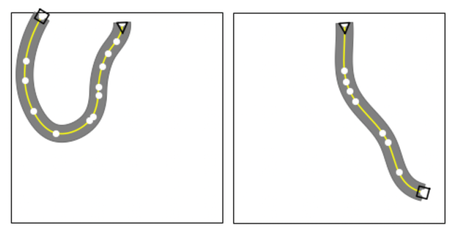
In this context, unsafe tests correspond to virtual roads that expose problems in the ego-vehicle while driving autonomously on them, for instance, causing it to drive off-road or invade the opposite lane. As discussed in the next Section, SDC-Scissor extracts a set of features from the road spine and road points that enable it to predict whether the corresponding virtual road will expose a problem in the ego-vehicle before the test execution.

SDC-Scissor relies on the open-source testing infrastructure developed for the CPS testing competition of the SBST (Search-Based Software Testing) workshop SBST:2021 . This infrastructure can automatically implement executable simulations from the road spines, execute them, and collect their results (e.g., pass/fail). We opted for this infrastructure for two main reasons: (1) It utilizes BeamNG.tech beamNG simulator; hence, it can execute physically accurate and photo-realistic driving simulations. (2) It has already been used to benchmark several automatic test generators (see SBST:2021 SBST2022 ); hence, it enables us to study the generality of SDC-Scissor. SDC-Scissor uses Frenetic DBLP:conf/sbst/CastellanoCTKZA21 as the main test generator, which uses a genetic algorithm for defining road points on a cartesian plane.

The open-source testing infrastructure developed for the CPS testing competition SBST:2021 enables driving agents to drive simulated vehicles and get programmatic control over running simulations (e.g., pause/resume simulations, move objects around). We consider two different driving agents as test subjects for our evaluation: The first is the driving agent shipped with the BeamNG.tech, which we refer to as BeamNG.AI, and the second, is an open-source trajectory planner, which we refer to as Driver.AI Gambi2019 . As explained by BeamNG.tech developers, a parameter called the “risk factor” (RF) controls the driving style of BeamNG.AI: low RF values (e.g., 0.7) result in smooth driving, whereas high RF values (e.g., 1.2 and above) result in an edgy driving that may lead the ego-car to “cut corners”. Driver.AI instead analyzes the road geometry and plans the car trajectory by computing for each turn the maximum safe driving speed ($v$) using the standard formula for centripetal force on flat roads with static friction ($\mu$) misc:safe-speed :

$$v=\sqrt{\mu\times r\times g}$$ (1)

where $r$ is the turn radius and $g$ is the free-fall acceleration.

Driver.AI relies on the user to provide the value of the friction coefficient, as well as information about the maximum acceleration and deceleration of the ego-car. In our evaluation, we estimated those values empirically following a trial-and-error approach. It is important to mention that, at the moment, both BeamNG.tech and Driver.AI do not have previous versions of their driving agents. This means that their behavior can only be altered or investigated by experimenting with the parameters already discussed in the context of our study. As a consequence, the target of our regression testing strategy is primarily focused on enabling SDC test selection, with the main goal of reducing the effort required to detect faults. For future work, assuming new versions of both BeamNG.tech and Driver.AI are delivered, we plan to experiment with consecutive versions of these AI agents so that it is possible to investigate the potential fault-detection capability of both of them.

2.3 Article Terminology

To avoid any confusion in terminology, it is important to note that in the rest of the paper, we will refer to simulation-based test cases generated by SDC-Scissor as test cases. Test cases are composed of virtual roads composed of a sequence of multiple road segments, as exemplified in Figure 1. Formally, road segments refers to (parametric) portions of roads of test cases; hence, they can be straight segments (no curvature), left turns (positive curvature), or right turns (negative curvature).

We refer to test cases that have been executed and evaluated in simulation as executed test cases. Then, if a test is passed successfully, we refer to it as a passing test, and if it failed, potentially revealing some issues with the system under test, we refer to it as a failing test.

On the other hand, as we elaborate more in the next sections, SDC-Scissor automatically assigns labels to the test cases regarding them being likely to fail or pass without executing them. In this context, we refer to the test cases which are considered by SDC-Scissor to be likely to pass as safe test cases and the ones that are considered likely to fail as unsafe test cases.

Regarding the features used in SDC-Scissor, static (road) features refer to any test case features that can be calculated without running any simulations, i.e., they are suitable for predicting test results (simulation results) before running simulation. As discussed in detail in the next section, we propose to use two different sets of road features: road characteristics and diversity metrics.

Regarding the experiments to answer RQ₂, we will discuss offline experiments that involves test selection from a previously generated (offline) pool of test cases in Section 4.2.2. We conducted the offline experiment in two experimental setups that mimic the issues of having a limited testing budget in the context of SDCs: 1) FIX, in which the amount of total test cases that can be executed in the simulation environment is fixed to a certain number. 2) REACH in which we continue executing the test cases until we reach a certain number of failing tests.

As discussed later in Section 5.3, we complement RQ₂ evaluations with real-time experiments, in which we study the application of SDC-Scissor to automated test generation, i.e., the test pool is being generated in real-time, and only the unsafe tests are being kept and executed. There, we have two experimental setups: 1) with a pre-trained ML model. 2) with an adaptive ML model that could be retrained with the correct labels of the generated test cases.

3 The SDC-Scissor Approach

In this section, we first overview SDC-Scissor’s software architecture and its main usage scenarios (Section 3.1); next, we describe the selected features used as inputs to SDC-Scissor (Section 3.2); finally, we explain how SDC-Scissor uses these features to classify test cases before executing them (Section 3.3).

3.1 SDC-Scissor Architecture Overview

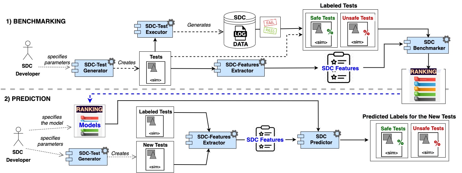
SDC-Scissor supports two main usage scenarios: Benchmarking and Prediction. In the Benchmarking scenario, SDC developers (or testers) leverage SDC-Scissor to determine the best ML model(s) to classify SDC simulation-based tests as safe or unsafe. In the Prediction scenario, instead, SDC-Scissor uses the most promising ML model(s) to classify newly generated test cases.

SDC-Scissor Software Architecture (Figure 2) implements these scenarios by means of five main software components, which have the main following responsibilities and relations:

1. SDC-Test Generator generates SDC simulation-based test cases.

2. SDC-Test Executor executes the tests and stores the test results, i.e., safe or unsafe labels, to allow training of the ML models.

3. SDC-Features Extractor extracts the input features from the SDC simulation-based test cases.

4. SDC-Benchmarker uses these features and collected labels to train the selected ML models and determines which ML model best predicts the tests that are more likely to detect faults.

5. SDC-Predictor uses the trained ML models to classify newly generated test cases, thus achieving cost-effective SDC simulation-based testing via test selection.

Figure 2: Overview of SDC-Scissor’s Software Architecture

3.2 SDC Test Case Features

SDC Test Case Road Characteristics - Features Set 1 (Used in RQ1, RQ2, and RQ3). To predict whether test cases are likely to result in safe or unsafe test cases before their execution, we use a set of simple static features extracted from the global characteristics (we refer to Road Characteristics) of the virtual roads used as test cases. We extract two types of Road Characteristics describing the main road attributes (see Table 1) and descriptive statistics about the road composition (see Table 2). Exemplary road attributes we consider are the total length of the virtual road, its starting and target positions on the map, and the count of left and right turns. To calculate road statistics, instead, we adopt the following procedure: (1) We extract the driving path that the ego-car must follow during the test execution; this path defines the test case and contains the road segments that the ego-car must traverse to reach the target position from the starting position. (2) We extract the metrics such as segment length, road angle, and pivot radius from the road segments. (3) We compute descriptive statistics by applying standard aggregation functions (e.g., minimum, maximum, average) on the collected road segment metrics.

Table 1: Road Attributes extracted by the SDC-Features Extractor. In the table, we report for each feature their name, description, and range (based on the tests in the generated datasets)

. Feature Description Range Direct Distance Euclidean distance between start and finish (Meters) [0 – 489.9] Length Total length of the driving path (Meters) [50.6 – 3317.9] Num L Turns Number of left turns on the driving path [0 – 18] Num R Turns Number of right turns on the driving path [0 – 17] Num Straight Number of straight segments on the driving path [0 – 11] Total Angle Cumulative turn angle on the driving path [105 – 6420]

Table 2: Road Statistics extracted by the SDC-Features Extractor. In the table, we report for each feature their name, description, and range (based on the tests in the generated datasets).

Feature	Description	Range
Median Angle	Median turn angle on the driving path	[30 – 330]
Std Angle	Standard deviation of turn angles on the driving path	[0 – 150]
Max Angle	Maximum turn angle on the driving path	[60 – 345]
Min Angle	Minimum turn angle on the driving path	[15 – 285]
Mean Angle	Average turn angle on the driving path	[52.5 – 307.5]
Median Radius	Median turn radius on the driving path	[7 – 47]
Std Radius	Standard deviation of turn radius on the driving path	[0 – 22.5]
Max Radius	Maximum turn radius on the driving path	[7 – 47]
Min Radius	Minimum turn radius on the driving path	[2 – 47]
Mean Radius	Average turn radius on the driving path	[5.3 – 47]

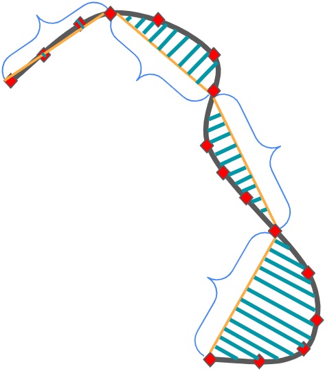
SDC Test Case: Diversity Metrics - Features Set 2 (Used in RQ3). To predict whether test cases are likely to result in safe or unsafe test cases before their execution, we also designed a new set of road features called Diversity Metrics. Specifically, we calculate per road segment the area that is spawned between the direct line of a segment (start and end of the segment) and the actual road. The concept of the diversity feature is also explained in Figure 3, where the green area represents the diversity of a single road segment. The curly braces indicate the segments of the road. A segment consists of road points marked as red diamonds. Furthermore, the yellow lines represent the direct paths between the start and end points of each segment. Concretely, we used for the calculation of the area Shapely Shapely , an open-source library for Python to perform geometric calculations. For each identified segment, we define a Shapely Polygon object that includes the road points and the line representing the direct segment line. All classes of Shapely provide a similar interface as well for calculating the area of a Shapely object. The previously constructed Polygon has a property called area. With this approach, we retrieve the area (also known as diversity in our context) of the segments. On this basis, we calculate two additional features; (i) Full Road Diversity, and (ii) Mean Road Diversity. As described in Table 3, the Full Road Diversity is computed by summing up all areas spawned by each segment of a road, whereas the Mean Road Diversity feature is the mean value of all areas of a single road. The main assumption for using these new features is that the road is more diverse if the spawned area is greater and, therefore, unsafer.

Table 3: Diversity features extracted by the SDC-Features Extractor. In the table, we report for each feature their name, description, and range (based on the tests in the generated datasets).

Feature	Description	Range
Full Road Diversity	The cumulative diversity of the full road composed of all segments.	[0 – $\infty$]
Mean Road Diversity	The mean diversity of the segments of a road.	[0 – $\infty$]

Figure 3: Road diversity as area (green) between the road (black) and direct segment line (yellow).

5

3.3 The SDC-Scissor’s Workflow

As described in Section 2, SDC-Scissor’s leverages an existing, open-source, and extensible SDC testing infrastructure to execute the test cases (SDC-Test Executor). Likewise, it relies on existing test generation algorithms integrated with that infrastructure to automatically generate the test cases to optimize (SDC-Test Generator). Hence, SDC-Scissor can already be used to improve the cost-effectiveness of several test generators.

During Benchmarking, SDC-Scissor utilizes SDC-Test Generator and SDC-Test Executor to collect the necessary data for training the ML Models, i.e., labeled test cases; next, it relies on SDC-Benchmarker to determine the ML models that best classify the SDC test cases as safe or unsafe as described below. Given a set of labeled test cases and the corresponding input features extracted by SDC-Features Extractor, SDC-Benchmarker trains and evaluates an ensemble of standard ML models using the well-established sklearn library. Next, it assesses each ML model’s quality using K-fold cross-validation and the whole dataset. Finally, it identifies the best-performing ML models according to Precision, Recall, and F-score metrics Birchler2022Cost and outputs the best (trained) models as well as the features needed to operate them.

SDC-Scissor can work with various ML models. In this study, we consider ML models that have been successfully used for defect prediction or other classification problems in Software Engineering  Bezerra ; Kaur ; PanichellaSGVCG15 ; SorboPASVCG16 ; RANI2021111047 ; PanichellaR20 . Specifically, we consider Naive Bayes (that applies Bayes’ theorem to train a probabilistic classifier) Caruana06anempirical , Logistic Regression (that uses a logistic function to model the probability of observing a certain class) ref1 , J48 (that creates a decision tree following the well-known C4.5 algorithm) Weka ; UAV:2022 , and Random Forests (that uses an ensemble of decision trees) TinKamHo1998 .

During Prediction, SDC-Scissor takes as input the (trained) ML Models and the definition of the features needed to use them. Next, it generates new test cases using SDC-Test Generator and utilizes SDC-Features Extractor to extract the necessary features. Finally, it invokes SDC-Predictor for classifying safe or unsafe test cases before executing them.

In the next section, we describe the studies we conducted to evaluate the benefits of using SDC-Scissor for test selection in the context of SDCs. After that, we present and discuss the achieved results.

4 Study Design

In this paper, we investigate Machine Learning-based test selection techniques for improving the cost-effectiveness of simulation-based testing of SDCs.

The first challenge (RQ₁) we focus on is to investigate whether, and to what extent, it is possible to classify test cases for SDCs as safe or unsafe before executing them, i.e., only considering input features, such as the one discussed in Section 3 by conducting offline and real-time experiments. Specifically, we investigate the use of ML models for classifying test cases in the context of Lane Keeping systems (see Section 2).

The second challenge we focus on is devising techniques that effectively leverage features extracted from SDC test cases to reduce testing costs while keeping testing effectiveness high. Hence, we investigate whether SDC-Scissor improves the cost-effectiveness of simulation-based testing of SDCs, compared to baseline approaches (RQ₂).

A further aspect we investigate is whether there is an upper bound on the precision and recall achieved by ML techniques in identifying SDC safe and unsafe test cases when using static SDC features (available before executing the tests). Hence, we focus on investigating whether fine-tuning the ML algorithms (e.g., calculating derived features and performing hyper-parameter tuning) improves SDC-Scissor’s ability to discern safe test cases from unsafe ones (RQ₃).

Finally, to investigate the practical usefulness of SDC-Scissor, we integrated our tool into the context of an industrial organization in the automotive domain (details of such an investigation are reported in Section 6).

In the following sections, we describe the dataset used in our study and the steps we followed to address these challenges.

4.1 SDC Test Cases Dataset Preparation

To enable the prediction of safe and unsafe SDC test cases, we used SDC-Scissor for executing the generated test cases and collected labels (safe/unsafe) from the test results (pass/fail). As reported in Table 4, we generated a dataset with $14,175$ data rows with full road features that are obtained from simulations of 8,500 tests using two driving agents and four configurations. What can be observed from the table is that SDC-Scissor takes AI engines’ inputs to generate the test cases, this lead to test cases having different configurations of roads and, as a consequence, different sets of road segments composing them. The test cases, their labels, and the SDC features characterizing them are the main data used for conducting our experiments. An overview of the data is reported in Table 4.

Table 4: Dataset Summary of SDC test cases on segment level and full road level (composed by segments).

Test Subject	Feature Set	Data Points
		Unsafe	Safe	Total
BeamNG.AI cautious	Full Road	312 (26%)	866 (74%)	1’178
BeamNG.AI moderate	Full Road	2’543 (45%)	3’095 (55%)	5’638
BeamNG.AI reckless	Full Road	1’655 (96%)	74 (4%)	1’729
Driver.AI	Full Road	1’045 (19%)	4’585 (81%)	5’630
				14’175
BeamNG.AI moderate	Road Segment	2’543 (3%)	72’433 (97%)	74’976
Driver.AI	Road Segment	2’494 (3%)	71’145 (97%)	73’639
				148’615

4.2 Research Method

We designed a set of experiments to answer our research questions:

• Machine Learning-based Experiments (RQ₁): The first set of experiments investigates whether ML models trained with the selected SDC test case features can identify safe and unsafe test cases before their execution.

• Offline Experiments (RQ₂): The second set of experiments investigates if and how much SDC-Scissor improves the cost-effectiveness of SDC simulation-based testing compared to baseline approaches.

• Real-Time Experiments (RQ₂): In these experiments, we train an adaptive model based on data observed while executing the tests and compare it with a pre-trained model.

• Optimization Experiments (RQ₃): The third set of experiments investigates how SDC-Scissor performance improves by adding new SDC features and tuning ML Models hyperparameters. Specifically, in RQ₃, we focus on investigating whether there is an actual upper bound on the precision and recall achieved by the ML techniques in identifying SDC safe and unsafe test cases when using static SDC features (available before executing the tests).

4.2.1 Machine Learning-based Experiments (RQ₁)

In the context of RQ₁, we study whether ML models can be used to predict safe or unsafe test cases and which combinations of features allow us to achieve more accurate predictions. As discussed in Section 3, we integrated into SDC-Scissor several ML models, and in the context of our work, we experimented with Logistic Regression Tolles2016 , the J48 Weka , the Random Forest TinKamHo1998 , and the Naive Bayes Caruana06anempirical as ML models.

We trained the ML models mentioned above using a training and test sets split strategy for each of the configurations listed in Table 4 separately. We evaluated the performance of each ML model by computing the standard metrics of precision, recall, and F-score Baeza-YatesR2011 ; Bezerra ; Ceylan ; Kaur ; CanforaLPOPP13 ; PanichellaSGVCG15 .

Rebalancing of training data. Since unsafe scenarios are an exception –not the norm– when generating random tests, the raw data we collected with SDC-Scissor is unbalanced toward safe cases. Therefore, we re-balanced the training data (in the case of the training and test sets split strategy) to avoid skewed distributions that would otherwise bias the ML models towards one specific class. Specifically, we adopted random oversampling, a re-balancing technique proven to be robust 10.5555/3000292.3000304 , to supplement the training data with multiple copies of some of the minority classes.

Size of the training dataset. To study how the training set size affects the ML models’ performance, we created balanced training datasets of increasing size (Table 5). However, we generated the test datasets to evaluate the ML models by randomly sampling the data point not included in the training datasets. Notably, we did not re-balance the test datasets to preserve the underlying distribution classes in the data.

Table 5: Model Training Dimensions

Dimension	Description	Dimension Configurations
Dataset	Using different datasets to train the model	BeamNG.AI (RF 1,1.5,2), Driver.AI, and Combined Datasets
Training Set	Changing training set size by using different percentage split for training and test sets	40% training set & 60% test set; 50% training set & 50% test set; 60% training set & 40% test set; 80% training set & 20% test set.

We also study the effects of different training strategies on each ML model’s performance. To do so, we evaluated the ML models using standard K-fold cross-validation Refaeilzadeh2009 . In particular, we set $K=10$ (i.e., 10-fold cross-validation) and utilize all the available data in each configuration.

4.2.2 Offline Experiments (RQ₂)

To answer RQ₂, we investigate whether SDC-Scissor improves the cost-effectiveness of simulation-based testing of SDCs, compared to baseline approaches. The quality focus is to understand whether SDC-Scissor reduces the time dedicated to executing safe (irrelevant) tests without affecting testing effectiveness (i.e., its ability to identify unsafe tests) compared to such baselines.

SDC-Scissor can use pre-trained models to classify safe and unsafe test cases. Therefore, we designed experiments to analyze how using pre-trained ML models for selecting (existing) test cases improves regression testing. For those experiments, we consider the combinations of ML models and features that achieve the best results in the context of RQ₁ (see Section 5.1). In addition, we contextualize the results achieved by SDC-Scissor using a baseline approach that performs a random selection of test cases. Notably, random selection is considered one of the standard baselines for evaluating test selection strategies Shin2018 ; Yoo:2010 . Finally, we also compare SDC-Scissor against a slightly more intelligent baseline approach that selects test cases by ordering the test to be executed considering their road length (in decreasing order). The conjecture of this second baseline is that the longer the road, the higher the probability of observing a fault.

Table 6: Offline Experiment Dataset

Dataset	Number of Safe Tests	Number of Unsafe Tests
Complete Set	3095	2543
Training Set	2034	2034
Test Pool (95/5)	1061	55
Test Pool (80/20)	1061	265
Test Pool (60/40)	763	509
Test Pool (30/70)	218	509

Studying the effectiveness of SDC-Scissor offline requires test cases and executions; therefore, we used a dataset with known test execution times. Due to the lack of backward compatibility of BeamNG.tech, we generated a new dataset for complementing our evaluation (see Table 10) involving the usage of the most recent version of BeamNG.tech. For all other evaluations, we used the data as reported in Table 6. In summary, the separated new dataset consists of $3^{\prime}559$ with $2^{\prime}225$ safe and $1^{\prime}334$ failing tests labeled with the BeamNG.AI (RF 1.5). As reported in Table 6, we created a Training Set, accounting for 80% of the whole data set, and we used the remaining 20% of data for testing. We created a balanced Training Set, but we purposely created four unbalanced Test Pools with different distributions of unsafe cases, ranging from few (5% of the testing data) to many (70% of the testing data). In creating our test pools, we under-sampled safe test cases (e.g., Test Pool (30/70)) since the number of unsafe test cases was inferior to the total amount of test cases in our complete dataset. Our conjecture is that using different Test Pool compositions allows us to assess SDC-Scissor’s performance in various settings.

Figure 4: FIX Experiment Overview.

Experimental setups of offline experiments. We conducted the offline experiment in two experimental setups, referred to as FIX and REACH. Since they mimic the issues of having a limited testing budget in the context of SDCs, We believe they are representative. We repeated the experiments in both setups $30$ times to increase the confidence in the achieved results.

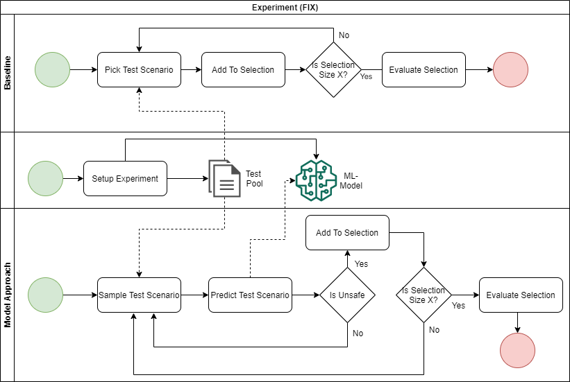
The FIX setup investigates the benefits of using SDC-Scissor when the resources allocated for testing are limited, i.e., the amount of test cases that can be executed in the simulation environment is fixed to a value $S$ (e.g., $S=5,6,etc.$). The process we followed to experiment with the FIX setup is illustrated in Figure 4 alongside the baseline processes. The baseline approach draws tests from the test pool (randomly or by considering their road length) and adds them to the test suite until the test suite reaches the target size $S$. SDC-Scissor, instead, samples the tests from the test pool but adds them to the test suite only if the ML model predicts that they are unsafe; as before, the process ends when the test suite reaches the target size $S$. In this setup, more effective techniques select larger portions of unsafe tests; therefore, we evaluate the performance of SDC-Scissor using the ratio of unsafe to safe test cases in the final test suites compared to the baseline approaches.

Figure 5: REACH Experiment Overview.

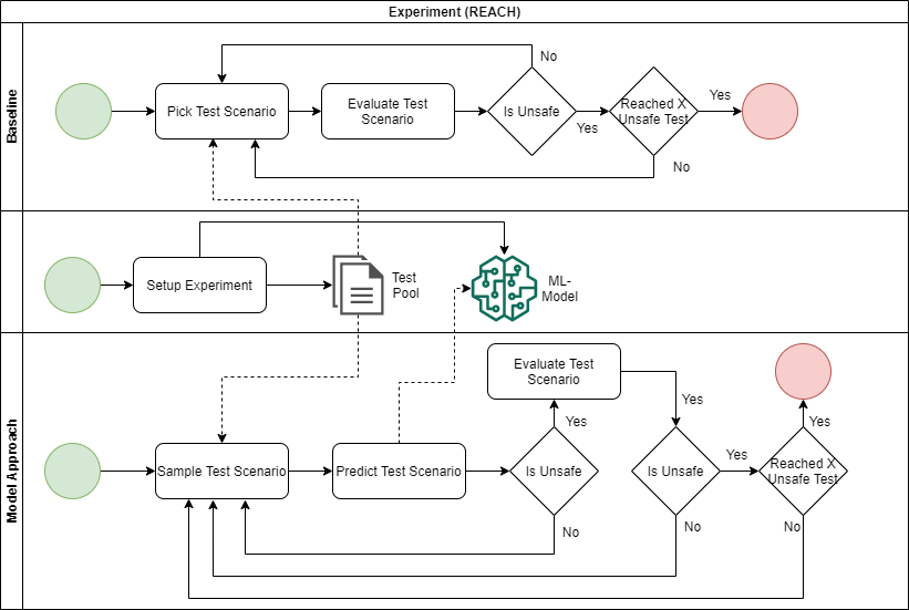
The REACH experiment, instead, investigates the ability of SDC-Scissor to reduce the time to identify at least $N$ unsafe test scenarios. In our experiment, we set $N=10$ since the time to identify that many unsafe test cases potentially requires the execution of many more (safe) test cases. The process we followed to experiment with the REACH setup is illustrated in Figure 5 alongside the random baseline approach. As before, the baseline randomly samples tests from the test pool and executes them until $N$ unsafe tests have been identified. REACH, instead, executes only those tests that are predicted to be unsafe by the ML models. In this setup, more effective techniques identify $N$ unsafe tests sooner; therefore, we consider the number of true positives (TP), true negatives (TN), false positives (FP), and false negatives (FN) predicted by the ML models. Having information about TP, TN, FP, and FN enables us to count how many tests were needed to reach the goal, how long it took to do so, and how much time was wasted in evaluating safe test cases.

4.2.3 Real-Time Experiments (RQ₂)

We complement the previous Offline Experiments to answer RQ₂, which focuses on applying SDC-Scissor to regression test case selection, with Real-Time Experiments in which we study the application of SDC-Scissor to automated test generation.

We conducted the Real-Time Experiments according to the following procedure: (i) SDC-Scissor to generate random test cases; (ii) for each newly generated test case, SDC-Scissor classifies it as safe/unsafe; and, (iii) we filter out test cases classified as safe before generating the next test case, whereas we executed the test cases classified as unsafe. As the test subject, we used BeamNG.AI in the moderate configuration (RF equal to 1.5) as this configuration is a compromise between overly conservative and overly aggressive driving styles.

A cost-effective test generator devotes more time to executing (likely) unsafe tests that can expose defects rather than executing safe test cases, which might not contribute any additional insight into the behavior of the SDC under test. Correctly identifying unsafe test cases, therefore, is paramount and depends on the quality of the ML model used as a classifier which, in turn, depends on the technique employed by the ML models and the data used to train them. Particularly relevant in this context is whether the ML model is predefined and fixed or allowed to be updated online as new data become available. The trade-off between these two configurations is that ML models have little operational costs once trained but may miss relevant behaviors; on the contrary, dynamically retrained ML models can cope with missing training data but at the cost of additional time spent in retraining them. Therefore, we compare the following two approaches:

• Pre-trained Model in which we used the best performing model identified during the Machine Learning-based Experiments (Section 5.1). We trained this model using the re-balanced dataset for the case of BeamNG.AI RF 1.5, as this is the configuration of the test subject used for this experiment.

• Adaptive Model in which we also used the best performing model identified during the Machine Learning-based Experiments (Section 5.1 but trained with only $60$ randomly generated test cases. After this initial training, we retrain the ML model after executing the predicted unsafe test cases using the newly collected ground truth labels for those test cases. Figure 6 illustrates this process. Notably, since the ML model may be inaccurate, this process collects both positive and negative labels.

Figure 6: Overview of the Adaptive Model configuration for the Real-Time Experiments.

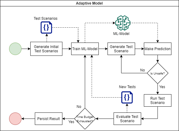
As before, we contextualize the results achieved by SDC-Scissor using a baseline approach that implements plain vanilla random generation, i.e., it does not filter the test cases.

We ran each configuration on a dedicated machine equipped with an Intel Core i5-6600K (3.5 GHz), 16 GB RAM, and an NVIDIA GeForce GTX 1070 GPU and set the test generation time budget to six hours.

During each execution of the experiment, we stored all the tests generated by SDC-Scissor so we could execute the test cases filtered out by SDC-Scissor post-mortem to calculate metrics such as accuracy, precision, and recall.

Table 7 provides an overview of the metrics used for the evaluation of SDC-Scissor across the various configurations. Those metrics include the count of unsafe tests found during each experiment (true positives), true negatives, false positives, and false negatives. Additionally, we consider how SDC-Scissor allocated the time budget to run safe and unsafe test cases, generate test cases, and rebuild the ML models.

Table 7: Evaluation metrics for the Real-Time Experiments.

Metric	Description	Range
Number of Unsafe Test Execution	The number of unsafe tests the approach simulated during the experiment	0-N
Number of Safe Tests Execution	The number of safe tests the approach simulated during the experiment	0-N
Time Allocation	How much time relative to the total time was spent with an action	0-1
True Positives/Negatives	Number of correct predictions for categories safe and unsafe	0-Number of Predictions
False Positives/Negatives	Number of incorrect predictions for categories safe and unsafe	0-Number of Predictions

In the second study, SDC-Scissor leverages real-time data (i.e., dynamically generated tests) and continuously (re-)trained ML models; this setup lets us evaluate the application of the proposed technique for automated test generation. As described before, in both setups, we compared the time-saving ability of SDC-Scissor with respect to the random selection strategy as well as its ability to detect more faults while allocating lower test execution costs.

4.2.4 Optimization Experiments (RQ₃)

RQ₃ investigates whether there is an upper bound on the precision and recall of ML techniques in identifying SDC safe and unsafe test cases when using SDC test case features available before executing the tests. A range of different optimization algorithms can be used to achieve potentially better results with respect to the default configuration of parameters of the ML models. Two of the most common hyperparameter tuning methods are Random Search and Grid Search 2986459.2986743 ; BergstraB12 ; AdnanAUR22 . Grid search performs better for spot-checking combinations that are known to perform well. Therefore, we experiment with Grid search as a hyperparameter optimization approach and investigate how SDC-Scissor’s performance improves when it employs fine-tuned ML models. Specifically, with Grid Search, we experimented with several parameter combinations for the best ML models using a 10-fold validation setting, as summarized below.

For the Decision Tree (J48) we covered all possible combinations of the following parameters:

• C (confidenceFactor): Is the confidence factor, and we experimented with values $[0.001,0.01,0.05,0.1,0.5]$

• M (minNumObj): Is the minimum number of instances in a leaf, and we experimented with values $[1,10,20,50,100]$

• R (reducedErrorPruning): Reduced error pruning is an alternative algorithm for pruning that focuses on minimizing the statistical error of the tree. We experimented with the following values $[yes,no]$

• S (subtreeRaising): This is a specific method of pruning whereby a whole set of branches further down the tree are moved up to replace branches that were grown above it. We experimented with the following values of it $[yes,no]$

For the Random Forest, we covered all possible combinations of the following parameters:

• I (numIterations): Is the number of trees in the forest, and we experimented with values $[5,10,100,1000,2000]$

• K (numFeatures): Is the max number of features considered for splitting a node, and we experimented with values $[0,10,100,500,1000]$

• depth: Is the maximum depth of the tree (0 unlimited), and we experimented with values $[0,5,10,20]$

• M (minNumObj): Is the minimum number of instances in a leaf , and we experimented with values $[1,10,20,50,100]$

For the Gradient Boosting, we covered all possible combinations of the following parameters:

• ’loss’ = [’log_loss’, ’deviance’, ’exponential’]

• ’learning_rate’ = [0.01, 0.1, 0.2, 0.4]

• n_estimators’ = [10, 100, 1000]

• ’criterion’ = [’friedman_mse’, ’squared_error’, ’mse’]

For the Logistic Regression, we covered all possible combinations of the following parameters:

• ’penalty’ = [’l1’, ’l2’, ’elasticnet’, ’none’]

• ’dual’ = [True, False]

• ’max_iter’ = [10, 100, 1000]

• ’solver’ = [’newton-cg’, ’lbfgs’, ’liblinear’, ’sag’, ’saga’]

For the Support Vector Machine, we covered all possible combinations of the following parameters:

• ’penalty’ = [’l1’, ’l2’]

• ’loss’ = [’hinge’, ’squared_hinge’]

• ’dual’ = [True, False]

It is important to note that we perform Grid Search (with a 10-fold cross-validation strategy) over all experiments (for a total of over 700 experimented combinations of parameters) and use the best combination of features and ML model from Section 4.2.1.

Section 5 elaborates on the achieved experimental results for all research questions, while Section 7 reflects on the results reported in such section, providing complementary insights, findings, and implications.

5 Results

This section presents the achieved results organized by research questions, while Section 7 discusses them in depth.

5.1 Machine Learning-based Experiments (RQ₁)

In this section, we discuss the results of RQ₁. Specifically, we describe the results achieved using the Road Characteristics listed in Section 3.2 as input features to build the ML models.

5.1.1 Machine Learning-based Experiments with Road Characteristics

We evaluated the ML models trained using Road Characteristics as the main SDC features with four splits of training and test data, as summarized in Table 5. However, for the sake of readability, we report here only the results achieved by the best-performing configuration, i.e., 80% training and 20% for testing. The full results can be found in our replication package RP2021 . Table 8 reports Precision, Recall, and F-score for both unsafe and safe labels separately to study how the ML models can classify each case (i.e., the experiments summarized in Table 5). It is important to note that in all experiments reported in Table 5, we rebalanced the training data (as discussed in Section 4.2.1).

Table 8: Performance of the ML models trained using road features. The results refer to the split of 80/20 between training and test data. The best results are shown in boldface.

Model	Unsafe Test Cases			Safe Test Cases
	Prec.	Recall	F1	Prec.	Recall	F1
BeamNG RF 1.5
J48	69.2%	67.4%	68.2%	61.5%	63.5%	62.5%
Naïve Bayes	79.3%	53.2%	63.6%	59.3%	83.1%	69.2%
Logistic	78.1%	65.3%	71.1%	64.8%	77.8%	70.7%
Random Forest	75.8%	62.7%	68.6%	62.5%	75.6%	68.4%
Driver.AI
J48	19.5%	64.1%	29.9%	82.9%	39.6%	53.6%
Naïve Bayes	20.3%	78.5%	32.3%	85.8%	29.8%	44.2%
Logistic	22.7%	56.5%	32.4%	85.0%	56.3%	67.7%
Random Forest	22.3%	52.6%	31.3%	84.4%	58.2%	68.9%

Regarding the BeamNG.AI dataset, with Risk Factor 1.5, the ML model performing the best in terms of F-score is Logistic (with 71% for both labels), followed by Random Forest (between 68%-69% for both labels). The other models, instead, achieved lower F-score values.

Regarding the Driving.AI dataset, we observe that the ML models achieved lower accuracy (49.1%) than the BeamNG.AI dataset. This result can be explained by looking at how unbalanced the Driver.AI dataset is since Driver.AI drives carefully, its dataset comprises mainly safe scenarios, and the predictions of the ML models tested on it are biased toward safe predictions.

Comparing the F-score achieved by the ML models against the Driver.AI and BeamNG.AI datasets shows this problem more evidently: the ML models performed comparably well for safe and unsafe classes against the BeamNG.AI dataset, whereas they performed well only for the safe test class in the case of Driver.AI. However, we can observe some similarities between all ML models in terms of F-score values when trained on the Driving.AI dataset and the BeamNG.AI dataset. For instance, for both datasets, Logistic and Random Forest tend to achieve better results. In both cases, and especially in the case of Driver.AI, most ML models struggle to classify safe test cases when compared to unsafe test cases.

Finding 1. SDC-Scissor is able to classify safe and unsafe test cases in both the BeamNG.AI and the Driving.AI datasets, with the Logistic and Random Forest models achieving the most reliable results in terms of F-score. However, all ML models achieved very poor results on the Driving.AI dataset (49.1%) when compared to the BeamNG.AI dataset. A result that we can justify by looking at the unbalance set of test cases in the Driver.AI dataset.

5.1.2 Analysis of Relevant Features.

Although the ML models trained using the road features can effectively classify the test cases as safe or unsafe, it is crucial to know the level of contribution of each of these features. We analyzed the road features for the BeamNG dataset discussed in Table 8 using two popular feature evaluation methods: information gain and correlation. While the detailed analysis results are reported in Appendix A, we summarise the main findings here.

Finding 2. The Road Characteristics extracted by SDC-Scissor contribute differently to identifying the safe and unsafe test cases. The Road Characteristics concerning the pivot radius (min, mean, std, median), the sum of the turn angles, the number of left and right turns, and the total length of the road are among the most important features, which are all belonging to the set of road features.

5.1.3 Impact of Risk Factor (RF)

To make it more clear how SDC-Scissor’s performance is affected by varying RF values, we compared its performance on BeamNG datasets with RF 1, 1.5, and 2 separately. While we report the details in Appendix B, here we summarise the main findings.

Finding 3. The accuracy of SDC-Scissor is influenced by their driving style and the diversity of datasets. For example, for more aggressive driving agents, the accuracy achieved by the ML models was higher than for cautious driving agents. Hence, predicting unsafe test cases is harder for cautious drivers than for reckless ones. Consequently, improving the testing of SDCs is more challenging for less aggressive driving agents.

5.1.4 Knowledge Transfer Between Different Driving Agents

We also studied the ability of the ML models to transfer knowledge from a driving agent to another one by training ML models with one AI’s dataset (BeamNG RF 1.5) and testing it with another AI’s dataset (Driver.AI) and vice versa. While we report the details in Appendix C, here we summarise the main findings.

Finding 4. Our results show that the knowledge is not transferable from one driving agent to another, i.e., SDC-Scissor performed worse when training ML models on data from a specific driving agent and testing them on data from a different one. However, ML models trained on the BeamNG data performed only slightly worse when evaluated on the Driver.AI data.

5.2 Offline Experiments (RQ₂)

In this section, we discuss the results of RQ2. Specifically, we focus on devising techniques that effectively leverage features extracted from SDC test cases to minimize testing costs while keeping testing effectiveness high. For this reason, we investigate whether SDC-Scissor improves the cost-effectiveness of simulation-based testing of SDCs, compared to baseline approaches (RQ2). Hence, we report the results of the FIX and REACH experiments (detailed in Section 4.2.2). Additionally, we report the results of the comparison between various ML models against the baseline approaches (described in Section 4.2.2) by considering different test pool compositions.

5.2.1 FIX Experiment results

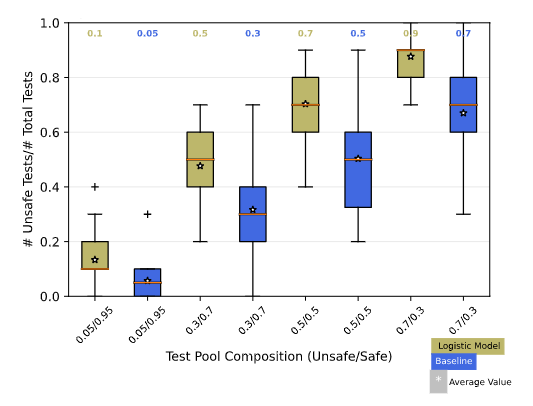
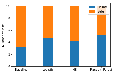
The goal of this experiment is to optimize the usage of the available resource in terms of testing execution time and effectiveness. Figure 7 compares the ratio of unsafe tests selected for execution using different ML models against the first baseline approach (random selection) across different test pool compositions. As can be observed from the figure, the Logistic model outperformed the baseline in all different test pool compositions (described in Section 4). Figure 8 illustrates that with fewer unsafe test cases in the pool, we observe improvements in the number of selected unsafe tests using ML models over the baseline. In the pool with the least unsafe tests, the Logistic model finds 133% more unsafe tests compared to the baseline approach. In the more balanced testing pool, Logistic finds 50% more unsafe tests, while with the pool with more unsafe than safe tests, it identifies 30% more unsafe tests. The Logistic model performs slightly better than the other models in all compositions except one (0.3/0.7), where Random Forest performed the best.

The confusion matrices in Table 9 further illustrate the concrete results in terms of effectiveness with the various pool compositions. In the pool with only 0.05 unsafe tests (Table 9-a), the Logistic model achieved 10 false negatives and 260 true negatives; this means that the model avoided the execution of 549 safe tests (considering that safe test cases take around 24 seconds in average to be executed), thus potentially reducing cost by more than 200 minutes in total on the less critical scenarios. However, the false-positive number is still high, with a cumulative 263 false-positives identified. As can be observed in Table 9)-b, for the Test Pool 0.7/0.3, the Logistic model achieved over 260 true positives and only 37 false positives. We observe that the precision correlates with the dataset composition; indeed, for datasets having more unsafe tests, the precision for unsafe tests is higher. For datasets having fewer unsafe tests, we obtain the opposite effect in the results. Figure 7 shows that the ML model performance and the baseline depend on the test compositions. The baseline and ML models perform better in test pools with more unsafe tests. Thus, according to our results, designing an appropriate test pool composition is of critical importance to achieving accurate prediction results.

Figure 7: Comparison Logistic Model and Baseline across different Test Pool Compositions.

Figure 8: Number of executed unsafe scenarios during the experiments on a)Test Pool(0.05/0.95) b) Test Pool(0.3/0.7) c)Test Pool(0.7/0.3)

a

b

c

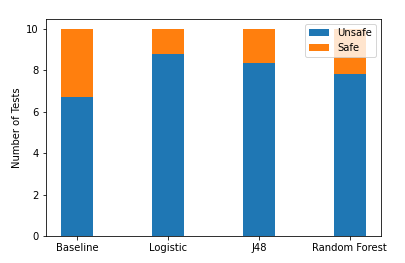
Finding 5. SDC-Scissor outperforms the random baseline approach in selecting unsafe tests across all test pool compositions, which is critical for more effective testing practices. In the test pool composition 0.3/0.7 (safe to unsafe), SDC-Scissor found 30% more unsafe tests; in the test pool composition 0.95/0.05 (safe to unsafe), instead, it found 133% more unsafe tests.

Table 9: Confusion Matrix for Logistic Model, cumulative over 30 rounds for a) Test Pool (0.05/0.95), b) Test Pool (0.7/0.3)

a Predicted class Unsafe Safe Actual Class Unsafe 40 10 Safe 260 549

b Predicted class Unsafe Safe Actual Class Unsafe 263 48 Safe 37 81

We assessed the cost-effectiveness of SDC-Scissor also against a second baseline whose selection strategy is based on the road length. The assumption is that the longer the road is the more likely it will be unsafe. In contrast to the random baseline, which selects the tests randomly from the test set, the second baseline orders the tests according to the road length and selects the longest ones. In Table 10, the cost-effectiveness of SDC-Scissor is compared to both baselines. The Random Forest and Logistic models have the best cost-effectiveness compared to both baselines with a selection of $80\%$ unsafe tests. On the other hand, the SVM and Naive Bayes have a worse selection than both baselines selecting only $40\%$ unsafe tests each, whereas the random and RL baselines select an average $42.6\%$ and $60\%$ unsafe tests, respectively.

Table 10: Cost-effectiveness ($\frac{\#failing}{\#passing}$) of SDC-Scissor against a random baseline and a road length-dependent baseline.

Model	Cost-effectiveness (Percentage of failing tests)
	SDC-Scissor	Random Baseline	RL Baseline
Random Forest	$4.0$ ($80\%$)	$0.7419$ ($42.6\%$)	$1.5$ ($60\%$)
Gradient Boosting	$1.5$ ($60\%$)	$0.7419$ ($42.6\%$)	$1.5$ ($60\%$)
SVM	$0.6667$ ($40\%$)	$0.7419$ ($42.6\%$)	$1.5$ ($60\%$)
Naive Bayes	$0.6667$ ($40\%$)	$0.7419$ ($42.6\%$)	$1.5$ ($60\%$)
Logistic Regression	$4.0$ ($80\%$)	$0.7419$ ($42.6\%$)	$1.5$ ($60\%$)
Decision Tree	$0.4286$ ($30\%$)	$0.7419$ ($42.6\%$)	$1.5$ ($60\%$)

Finding 6. SDC-Scissor outperforms a baseline approach that selects test cases based on their road length. The baseline has a cost-effetiveness of $1.5$ whereas the Random Forest and Logistic provide a cost-effectiveness of $4.0$ each.

5.2.2 REACH Experiment

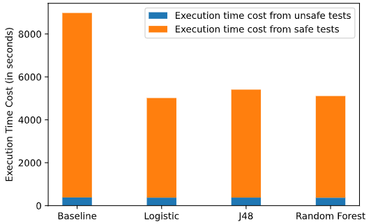
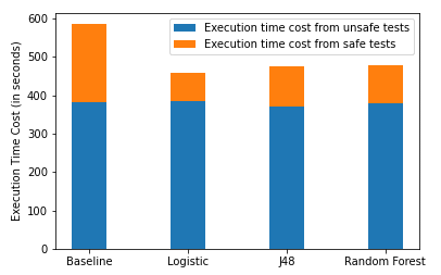
The goal of this experiment is to investigate whether the usage of ML models allows for reducing the total test execution time. By reducing the total test execution costs, a testing pipeline would be able to spend more testing time on more safety-critical test cases. The task in this experiment was to identify, as early as possible, ten unsafe tests while minimizing the number of total executed test cases. To perform the various comparisons, for each experimented strategy, we collected information about the number of test cases required to reach ten unsafe cases as well as the cumulative cost (i.e., the execution time) to run all the test cases (i.e., till the final unsafe scenario was identified). Further, we collected information concerning the execution time for both safe and unsafe test cases. The conjecture behind this analysis is that the testing cost concerning safe cases should as limited much as possible, whereas the test cost dedicated to unsafe cases is beneficial to identify flaws of SDC in virtual environments.

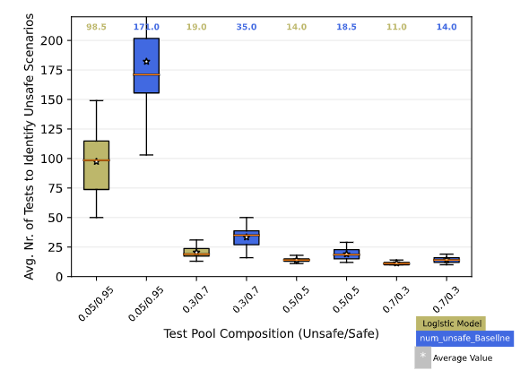
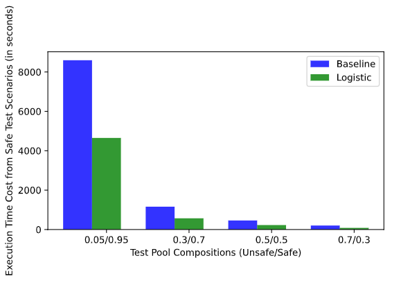
Figure 9 and Figure 10 provide an overview of the performance of the baseline compared to the Logistic model (the best-performing model in previous experiments) across different test pool compositions. Table 11 summarizes the results of the REACH experiment. We observed that the Logistic model performed better across all test pool compositions. The test costs strictly depend on the required numbered of tests to be executed before identifying the minimum set of 10 unsafe tests. Although the difference in the number of required tests tends to be higher in the pool with fewer unsafe tests (in the 0.05/0.95 pool between 171 to 98.5 tests, in the 0.7/0.3 between 14 to 11 tests), SDC-Scissor allows for reducing test execution time dedicated to less critical tests when the test pool presents more unsafe tests. Figures 11 show that in the smaller unsafe pool it is higher the test execution time dedicated to less critical tests. The test execution time for these less critical tests is 85% higher in the baseline than in the Logistic model. In the larger pool, the Logistic model selects 80% unsafe tests, whereas the baselines only have 42.6% and 60%, respectively.

Finding 7. We investigate whether SDC-Scissor can reduce the number of executed tests required to find at least N unsafe tests. Our results show that SDC-Scissor outperformed the baselines across all test pools, with the Logistic model reducing the unnecessary execution time dedicated to safe tests by selecting 80% unsafe tests, whereas the baselines select 42.6% and 60% unsafe tests, respectively. SDC-Scissor performed better compared to the baseline when test pools are characterized by fewer unsafe tests.

Figure 9: Comparing the Logistic model with the baseline across the different test pools.

Table 11: Results of the REACH experiments comparing the Logistic model and the baseline in various test pool compositions (safe/unsafe test ratio). Execution time is reported in seconds, and the values are averaged across the experiment repetitions.

Model/Pool	Tests #	Execution Time
		Safe	Unsafe
Smart Selector
Test Pool (0.05/0.95)	98.5	4664	375
Test Pool (0.3/0.7)	19	475	376
Test Pool (0.5/0.5)	14	214	389
Test Pool (0.7/0.3)	11	54	379
Baseline
Test Pool (0.05/0.95)	171	8079	382
Test Pool (0.3/0.7)	35	1243	383
Test Pool (0.5/0.5)	18.5	439	391
Test Pool (0.7/0.3)	14	193	387

Figure 10: Time spent for the execution of safe tests, Logistics vs. Baseline across different test pools

a

b

Figure 11: Time spent on executing each safe and unsafe test case for different models in a) test pool (0.7/0.3) b) test pool (0.05/0.95)

In Section 7, we discuss further results of RQ2, providing additional insights on this research question.

5.3 Real-Time Experiments (RQ₂)

In this section, we present the results of the real-time experiments, where we compare the results of a pre-trained model and a real-time model with the baseline approach.

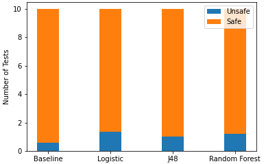
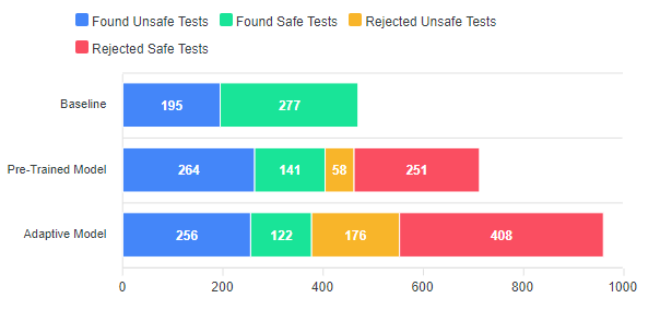
Baseline vs. Pre-trained and Adaptive Models. Figure 12 gives an overview of the results achieved by the experimented models. We observe that the baseline executed a higher number of test cases (472). The pre-trained model runs more test cases (405) than the real-time approach (378). Figure 12 summarizes our main observations, as elaborated in the next paragraphs.

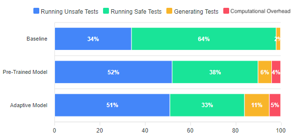
The pre-trained and real-time models apply a machine learning-based test selection, which leads to numerous rejected (i.e., non-executed) test cases: real-time and pre-trained experienced 588 and 309 rejected tests, respectively. The baseline uses 98% of the time to execute test cases; only 2% is dedicated to generating test cases. The pre-trained and real-time approaches use more time for test generation (6% pre-trained, 11% real-time approach). In addition to the longer test generation process, these two approaches allocate time for predictions and evaluation of tests (pre-trained 4%, real-time 5%), which the baseline does not need to perform. Compared to the pre-trained approach, the real-time approach continuously trains the machine learning model with new tests.

Interestingly, although the baseline executes more test cases, both pre-trained and real-time approaches found more unsafe test cases (baseline 195, pre-trained 265, real-time 256). The pre-trained model was able to find 35% more unsafe test cases, executing only 49% of safe tests. In Figure 12, we can observe that the baseline only spends 34% of the time running unsafe tests, while 64% of the test time was spent on executing safe test tests. In contrast, our proposed approaches dedicated more than 50% of the time to unsafe tests, which is positive since, in a testing environment, the goal is to find more errors in less time (in our case, it corresponds to exposing more weakness in SDC).

Finding 8. Our results show that even though the baseline approach executes more test cases, both the real-time and the pre-trained (i.e., offline) models integrated into SDC-Scissor are able to find more unsafe tests than the baseline. The time investment of predicting the outcome of test cases and generating more tests is beneficial for testing purposes. The pre-trained model was able to find 35% more unsafe tests than the baseline, with the baseline only dedicating 34% of the time budget to assessing unsafe tests. The offline model spends 52% running unsafe and only 38% on safe test cases.

a

b

Figure 12: Comparison of the metrics for different real-time approaches in a 6-hour run a) generated test cases distribution. b) spent time distribution across different tasks.

Table 12: Comparison between pre-trained and real-time models.

Model	Acc.	Unsafe		Safe
		Prec.	Recall	Prec.	Recall
Pre-trained Model	72.1%	65.2%	82%	81.2%	64%
Real-time Model	69%	67.7%	59.3%	69.9%	77%

Adaptive vs. Pre-trained Model. Figure 12 shows that the testing time allocation for the pre-trained and real-time models is similar, but the real-time model spends more time on test generation (11%) than the pre-trained one (6%). The pre-trained model is based on the previously generated dataset with 5,643 (consisting of 3,559 valid test descriptions as described in Section 4) test cases, whereas the real-time model started with generating an initial dataset of 60 test cases as described in Section 4. Table 12 shows that the pre-trained model achieved a higher accuracy (72.1%) than the real-time model (69%). The lower accuracy explains the higher number of test cases generated by the pre-trained model (tests generated; real-time 962, pre-trained 714). Although the pre-trained model has higher accuracy in general and higher unsafe recall, it only found 3.13% more unsafe tests than the real-time model.

Finding 9. The offline model achieved an accuracy of 72.1%, which is higher than the real-time model (69%). A real-time approach can achieve similar results compared to an offline model, with the real-time model finding only 3.13% fewer unsafe tests than the offline model. In achieving such results, the real-time model only used an initial set of 60 test cases, whereas the offline model leveraged 5,643 tests.

Training costs: Pre-trained and Adaptive Models v.s. Random Baseline. From a qualitative point of view, the cost of the training dataset is about 0 for the random baseline, while it is $>0$ for the pre-trained and adaptive Models. It is important to mention that, for all results discussed in Section 5.3 and for the adaptive and pre-trained models, we did not include the cost required for training the ML models on the training data. This choice was made since the cost of training the best ML model can be considered negligible compared to the cumulative cost of generating all tests and executing them. Indeed, the average cost to train the Logistic Regression model (i.e., the best ML model) on 60 test cases is of about 0.139 seconds, whereas the cost to train the same ML model on 5,643 tests (for the offline model) is of about 0.685 seconds. However, since for other ML models or particular settings of the same ML model (e.g., different from its standard configuration), we could achieve rather higher training costs, we discuss this topic in the threat to validity.

Training dataset preparation: Pre-trained and Adaptive Models v.s. Random Baseline. It is important to report that the comparison of SDC-Scissor and the random baseline does not take into account the time (i.e., the cost) required for the training dataset preparation in the real-time experiments. From a qualitative point of view, the cost of the preparation of the training data is about 0 for the random baseline (since no training is needed), while for the pre-trained and adaptive models, this has a non-negligible cost. The preparation of the training data includes: (i) the time required for the design, implementation, and testing of the road characteristics (i.e., one week of full-time work) into SDC-Scissor; (ii) and the cost for the automated extraction of such features from all test cases (158 seconds). In total, this required us (i.e., to the first author of this work around one week of work). Hence, while both the pre-trained and adaptive models are more cost-effective than a random baseline when selecting test cases, the training data preparation cost represents a very high cost to be sustained upfront, which becomes beneficial only over a long period of test execution time.

Table 13: Pre-trained Model, Confusion Matrix

		Predicted class
		Unsafe	Safe
Actual Class	Unsafe	264	58
	Safe	141	251

Table 14: real-time Model, Confusion Matrix

		Predicted class
		Unsafe	Safe
Actual Class	Unsafe	256	176
	Safe	122	403

5.4 Optimization Experiments (RQ₃)

In RQ3, we focus on investigating whether there is an actual upper bound of ML techniques in identifying SDC safe and unsafe test cases when using static SDC features (available before executing the tests). We performed Grid Search for the Random Forest, J48, Gradient Boosting, Logistic, Naive-Bayes, and Support Vector Classifier to identify the best hyper-parameters for each model. Table 16 summarizes the results of Grid Search by showing the F-score (F₁) for safe and unsafe test cases as well as the averaged F-score.

The best two models regarding the averaged F-score are the Gaussian Naive Bayes (F${}_{1}=60.0\%$) and the J48 Decision Tree classifiers (F${}_{1}=59.5\%$). Although these two models have similar averaged F-scores, they are distinct among the classes. Among the unsafe tests, the J48 Decision Tree achieved an F-score of $70.3\%$, but for the safe tests, it achieved $42.6\%$. In the case of the Naive Bayes model, we have among the unsafe tests an F-score of $41.0\%$ and $71.0\%$ for the safe tests.

Table 15: Best ML models with recall, precision, and F-score.

ML Technique	Precision		Recall		F1
	Safe	Unsafe	Safe	Unsafe	Safe	Unsafe
J48	$49.8\%$	$65.4\%$	$76.0\%$	$37.1\%$	$42.6\%$	$70.3\%$
Naive Bayes	$66.0\%$	$47.0\%$	$75.0\%$	$37.0\%$	$71.0\%$	$41.0\%$

For the best two models according to their averaged F-score, we show their corresponding confusion matrices in Figure 14 and Figure 14. Furthermore, a detailed overview of their precision, recall, and F-scores among the classes are reported in Table 15.

Both confusion matrices show a similar distribution. The models identify most of the true unsafe test scenarios with 1’677 and 1’650 cases, but in predicting the safe tests, the models have a low true positive rate with 409 and 516 correct predicted safe tests.

Finding 10. The Naive Bayes and J48 models reach a weighted average F₁ of 60%. Their confusion matrices show that they are able to predict unsafe tests, whereas their performance on detecting safe tests is less accurate.

Table 16: Best ML model configurations after a Grid search

ML Technique	Param. Config.	F1		Weighted avg. F1
		Safe	Unsafe
Random Forest	I=5,	35.1%	72.4%	57.8%
	K=10,
	depth=10,
	M=50
J48	C=0.5,	42.6%	70.3%	59.5%
	M=20
Gradient Boosting	criterion=friedman_mse,	77.0%	0.0%	48.0%
	learning_rate=0.01,
	loss=log_loss,
	n_estimators=10
Logistic	dual=False,	76.0%	12.0%	52.0%
	max_iter=10,
	penalty=none,
	solver=saga
Naive-Bayes	No parameters	71.0%	41.0%	60.0%
SVC	dual=False,	76.0%	28.0%	58.0%
	loss=squared_hinge,
	penalty=l2

Figure 13: Confusion matrix for the Gaussian Naive Bayes model.

Figure 14: Confusion matrix for the J48 Decision Tree model.

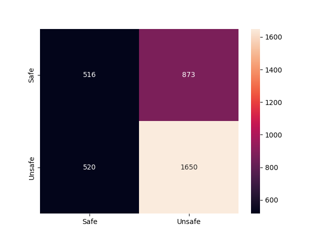
6 Integration of SDC-Scissor in the Industrial Use Case

6.1 Experiments involving an Industrial use Case (AICAS)

We investigate the extent to which SDC-Scissor can be integrated into the context of industrial organizations in the automotive domain, addressing one of the open questions in simulation-based testing 3533818 ; Birchler2022Cost ; Gambi2019 ; abdessalem2018testing for SDCs. We identified the AICAS company as an ideal use case for this investigation. AICAS develops JamaicaCAR, an OSGi-based technology for the automotive sector, currently running in more than five million cars worldwide. A pressing challenge for AICAS concerns the need to combine simulations and HiL testing protocols to optimize the testing costs. Specifically, AICAS aims to reduce testing costs by automatically generating inputs, i.e., signals, compatible with the Controller Area Network (CAN) Bus protocolcanbus-history in simulated environments.

Figure 15: AICAS’s Jamaica EDP validation setup.

Figure 16: Can Bus in the context of an SDC.

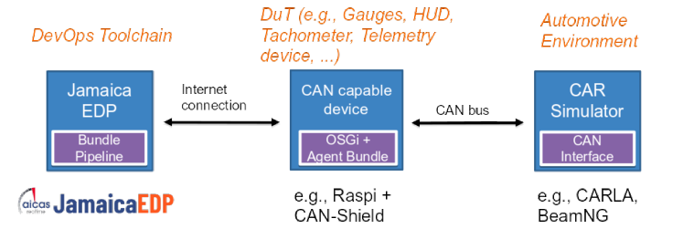
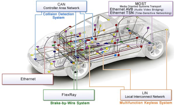
Based on the trajectories planned by the planning module of SDC, the control module of SDC typically takes charge of the longitudinal and lateral control of the vehicle and generates appropriate control commands (e.g., steering, acceleration, brake) that it sends to the related hardware component of the SDC via the CAN Bus (see Figure 16).

Figure 17: CAN Bus code pipeline integrated into SDC-Scissor

Figure 18: SDC-Scissor’s CAN Bus code pipeline: SDC Test Case Generation and Storage.

Figure 19: SDC-Scissor’s CAN Bus code pipeline: SDC Test Data Conversion & Generation of CAN Playback Data.

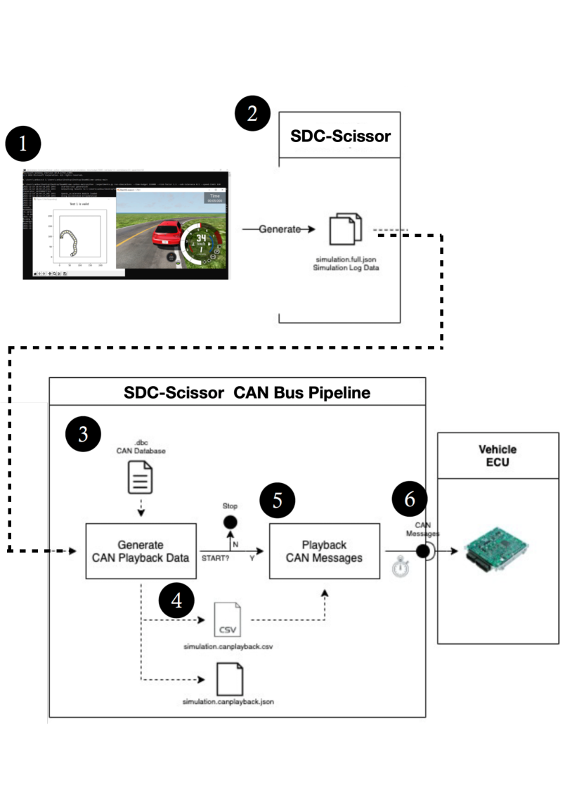
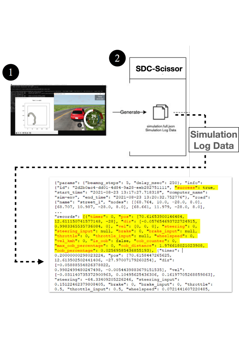
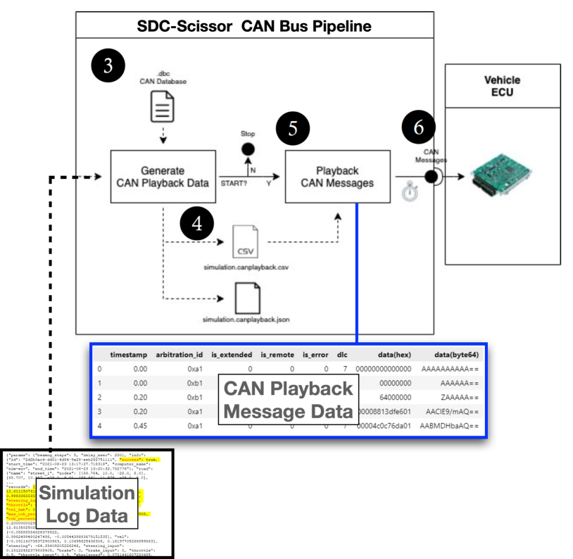
To allow validation of the described scenarios, AICAS provided us with devices under test (DuT) equipped to communicate via the CAN Bus. We connected the devices to the CAN bus and the CAN bus to a driving simulator that allowed us to generate the appropriate signals (see Figure 15). The devices act as a validation context for the described automotive scenarios.

There are several main advantages of integrating test cases generated by SDC-Scissor in the testing workflow of AICAS:

• Increased level of test automation: Currently, AICAS inputs are manually generated or designed by testers and developers in its organization. The usage of an integrated framework such as SDC-Scissor can enable the generation of test cases automatically, increasing automation and diversity of generated SDC scenarios.

• Increased level of realism: Most of the manually entered signals inserted in the Can Bus protocol by the testers and developers of the AICAS organization do not reflect a real driving set of signals (e.g., the provided acceleration and steering angle of the vehicle are not reflecting a real driving test scenario, which makes the used inputs in most cases too random or unrealistic).

Integration steps. To investigate the extent to which SDC-Scissor can be integrated into the context of AICAS, we extended SDC-Scissor with a CAN Bus code pipeline (see the full pipeline in Figure 17), which automates the following steps:

• SDC Test Case Generation and Storage (Steps 1-2): As visualized in Figure 18, we first use SDC-Scissor to generate 3,559 SDC test cases (with BeamNG, with RF 1.5 - moderate driving), execute them, and store the corresponding execution log in a JSON file (i.e., the actual simulation.full.json containing all information concerning the generated and executed tests by SDC-Scissor, see Figure 18), which constitutes the dataset of our experiments.

• SDC Test Data Conversion & Generation of CAN Playback Data (Steps 3-5): In this stage, we convert (and visualized in Figure 19) the execution log from the JSON file (i.e., simulation.full.json generated by SDC-Scissor to CAN Playback Data (i.e., the file simulation.canplayback.*).

• Transmission of CAN-based Signals (Steps 6): The messages (i.e., the CAN Playback Data) generated in the previous step are then transmitted to the CAN Device according to defined timestamps, consistent with the one generated by SDC-Scissor while executing SDC test cases. Specifically, referring to the specified used CAN database (i.e., ¡.dbc¿), we converted SDC-Scissor test case data (i.e., ¡simulation.file.json¿) to CAN messages (i.e., ¡simulation.canplayback.csv¿). Using a specified CAN interface device, logged CAN frames are played back to external CAN bus devices. These final steps allow us to finally send realistic SDC signals concerning the driving scenarios to the CAN Device (i.e., SDC test cases generated by SDC-Scissor) in an automated fashion).

From a technological point of view, the definition and implementation of the pipeline in Figure 17 required us to leverage the following libraries: (i) Python-CAN, which allows controlling various CAN interface devices in the Python environment; (ii) the cantools, which support CAN database encoding and decoding actions (from the device to the Simulator, and vice versa).

6.2 Industrial Use Case (AICAS): Integration results

To investigate the extent to which SDC-Scissor can be integrated into the context of AICAS, we extended SDC-Scissor with a CAN Bus code pipeline described in Section 6.1 and shown in Figure 17. The development and integration of this pipeline in the AICAS context required around five months of work: considering the time to design the pipeline till its implementation and integration, including the time for running all the required experiments reported in this article (this includes the generations of test cases by SDC-Scissor, their execution, the analysis of the data, etc.).

Table 17 reports the details of the test cases generated by SDC-Scissor. Specifically, we generated around 3,600 test cases, which required a total execution time of 12h, 17m, and 11s, with an average simulation time of 12.428 seconds for each test case and a max. observed simulation time of 21.4 seconds.

Table 17: Dataset Summary

Property	Value
Nr. SDC test cases Generated by SDC-Scissor (BeamNG RF 1.5)	3,559
Total Simulation Time	12h 17m and 11s
Average Simulation Time	12.428 s
Max. Simulation Time	21.4 s

The most challenging steps of the integration of SDC-Scissor into the context of AICAS are represented by the SDC Test Data Conversion & Generation of CAN Playback Data (Steps 3-5, shown in Figure 17) and the Transmission of CAN-based Signals (Steps 6, shown in Figure 17). The main aspect that made this task challenging was the need for signal conversions and mapping between SDC-Scissor’s signals and CAN Playback Data. As shown in Figure 20, for each signal generated by SDC-Scissor, we had to generate a corresponding value mapped with the CAN Playback module.

Based on the simulation-based signals generated by the implemented SDC-Scissor pipeline, we were able to generate appropriate control commands (e.g., steering, acceleration, brake), and send them to the related hardware component of the SDC via the CAN Bus. Table 18 reports the details of SDC-Scissor’s integration process. Specifically, for all 3,600 generated test cases, which required a total execution time of 12h, 17m, and 11s, it required a total of 52.391 seconds to SDC-Scissor for enabling the automated signal conversions, mapping, and transmission of CAN messages.

As visualized in Figure 21, it requires 14.721 ms on average to SDC-Scissor to translate simulation-based signals into CAN-compatible signals. In comparison with the current manual signal generation process, it requires on average 1-2 days for AICAS developers and testers to design and then generate a sequence of CAN signals corresponding to 10-15 test cases generated by SDC-Scissor (according to the qualitative assessment of our main contact people within AICAS). In addition to the test automation enabled by SDC-Scissor in the context of AICAS, the generation of a more realistic sequence of SDC signals (corresponding to signals of a realistic SDC car driving in a virtual test case) is vital for the identification of safety-critical scenarios to be executed and tested via the CAN Bus protocol.

Finding 11. The main challenging aspect of integrating SDC-Scissor into the context of AICAS was the need to systematically automate the mapping between SDC-Scissor’s signals and CAN Playback Data. Considering 3,600 generated test cases as input, it required a total of 52.391 seconds to SDC-Scissor for enabling the automated signal conversions, consisting of about 14.7 ms on average to SDC-Scissor to translate simulation-based signals in CAN-compatible signals of a single test case. The corresponding process of manually designing and generating the sequence of CAN signals corresponding to 10-15 test cases generated by SDC-Scissor takes between 1-2 days for AICAS developers and testers.

Figure 20: Mapping between SDC-Scissor’s signals and CAN Playback Data

Table 18: Results of the Integration Process

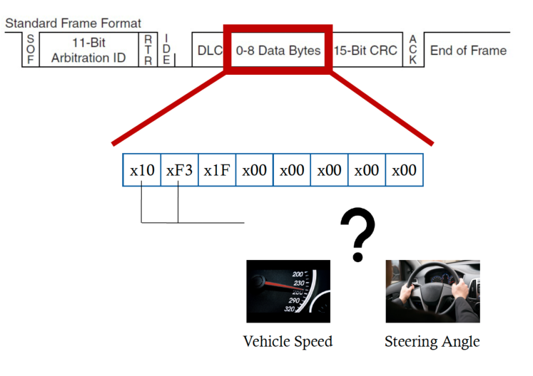
Property	Value
Nr. SDC test cases Generated by SDC-Scissor (BeamNG RF 1.5)	3,559
Total Conversion of Messages + Transmission of CAN signals	52.391 s
Mean Time for Conversion of Messages + Transmission of CAN signals (per each SDC test case)	14.721 ms
Min Time for Conversion of Messages + Transmission of CAN signals (per each SDC test case)	7.892 ms
Min Time for Conversion of Messages + Transmission of CAN signals (per each SDC test case)	30.006 ms

Figure 21: Performance of Conversion and Transmission time.

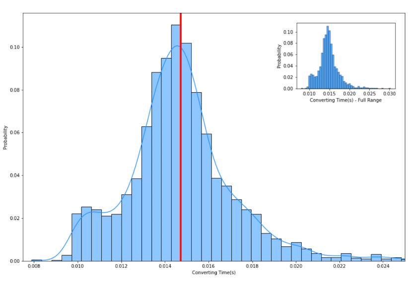
7 Discussion

This section discusses additional factors that can influence the results of the various research questions, providing more insights and findings about them. Moreover, it also provides a concrete discussion on directions for future research in the field.

7.1 Discussion of Experiments Using Road Characteristics as Input Features to the ML Models

As we have observed from the conducted experiments in RQ₁, SDC-Scissor is able to classify safe and unsafe test cases in both the Driving.AI dataset and the BeamNG.AI dataset, with the Logistic and Random Forest models achieving the most reliable results in terms of F-score values for labels. Moreover, we also observed that the Road Characteristics extracted by SDC-Scissor contribute differently to identifying the safe and unsafe test cases. The Road Characteristics concerning the pivot radius (min, mean, std, median), the sum of the turn angles, the number of left and right turns, and the total length of the road are among the most important features, which are all belonging to the set of road features.

In the context of RQ₁, there are other factors that can impact the results of SDC-Scissor, such as (i) the risk factor (RF) of the SDCs; (ii) the ability of the ML models to transfer knowledge from a driving agent to another one (i.e., between BeamNG RF 1.5 dataset and the Driver.AI dataset); finally, (iii) we complement the previous Offline Experiments, which focus on applying SDC-Scissor to regression test case selection, with Real-Time Experiments in which we study the application of SDC-Scissor to automated test generation.

7.2 Further Remarks and Future Directions

This work can have relevant implications for developers and researchers. Hence, this final discussion reflects further remarks on the results of all questions, with a specific focus on future directions of RQ₃ and RQ₄ for developers and researchers.

For what concerns developers, the designed tool allows identifying specific problems that need to be carefully monitored in simulation environments at the time of testing. These include, for instance, the need for coping with testing multiple hardware versions and diversified test inputs to verify correctness with realistic test inputs. Also, it is of paramount importance to be able to generate inputs that lead to a different safety-critical situation in a safe manner (i.e., without harming humans). SDC-Scissor allows to generate and identify test cases that can cause the SDC to fail by using different safety criteria (in the context of this work, we focus on the line-keeping feature as the main safety criterion, but further criteria can be easily integrated and tested).

The integration of SDC-Scissor into the AICAS use case allows us to demonstrate that the proposed approach can automate the testing process of such a large automotive company, coping with the need to complement their hardware-based simulation (based on the Can Bus protocol) with simulation-based testing automation. Specifically, SDC-Scissor allows addressing two pressing challenges of AICAS such as the need for (i) an Increased level of test automation (e.g., AICAS inputs are manually generated or designed by testers and developers in its organization) with test cases automatically generated to increase the diversity of generated SDC scenarios; (ii) and the need of Increase level of realism, since most of the manually entered signals inserted in the Can Bus protocol by the testers and developers of the AICAS organization do not reflect a real driving set of signals (e.g., the provided acceleration and steering angle of the vehicle are not reflecting a real driving test scenario, which makes the used inputs in most cases too random or unrealistic).

To enable the detection and fixing of SDC bugs during the evolution of SDCs, developers can focus on configuring SDC-Scissor to test different combinations of simulators, and AI agents in diversified testing cases, to identify faults in the AI engine and the connected hardware of the system. Of course, we expect that test cases for assessing and detecting SDC bugs can vary between different organizations. To perform such new experiments, SDC-Scissor can be used to generate new test cases by increasing the level of realism of the generated simulation by including obstacles in the generated tests. This is to observe the behavior of the SDCs as well as the ability of SDC-Scissor to identify safe and unsafe test cases in the context of more articulated test cases.

From the discussion of the results of RQ₃, we identified that there is an upper bound of the extent to which static SDC features (i.e., features available before executing the tests) can be used to predict SDC testing outcomes. This represents a relevant topic for both developers and researchers for future investigation. From one side, we may argue that novel static SDC features need to be designed to achieve better results (in terms of precision, recall, and F-score). On the other side, we also observed in RQ₃ how the usage of different SDC features and hyperparameter optimization strategies do not lead to drastically better results. Given the complexity of the simulation environment and its simulated physics, we argue that to cope with the upper bound of static SDC features, better results can be achieved by combining static metrics and runtime SDC metrics (i.e., metrics available during the execution of SDC test). The rationale of such implication is that there is limited information that can be used to derive if SDC test cases will fail or not before their execution, and achieving better results requires designing metrics that are available during the execution of test cases. For instance, one could consider using the average distance, speed, and steering angle in the proximity of an SDC failure (namely, a crash or a violation of the safety criterion, such as the lane-keeping feature).

For what concerns researchers, this work triggers activities towards better testing and analysis of SDCs. First and foremost, given the identified safe and unsafe test cases, it can be used to derive higher-order JiaH09 SDC-specific mutation operators. For example, the integration of obstacles and different fault detection strategies related to other safety criteria (different from the lane-keeping feature) during the execution of test cases could lead to mutants that change the test case outcome towards more faulty SDC behaviors. More complicated would be dealing with runtime adjustments of SDC test cases, which may require to be instantiated by perturbing the SDC behavior during the testing process.

Also, the work could foster the development of specific static analysis tools for SDC, looking for SDC-specific recurring problems observed in failing test cases. Complementary empirical research could be directed to investigate the difficulty (e.g., duration) of fixing SDC-specific bugs and developing tools guiding developers in allocating the appropriate development effort to various types of SDC bugs. In the context of SDCs, the usage of SDC-Scissor can help researchers (and developers) have a deep knowledge of SDC bugs and their root causes, which is potentially facilitated by their high reproducibility. Specifically, being able to reproduce a bug is crucial during bug triaging and debugging tasks but not always possible in field testing BettenburgJSWPZ07 ; HuangZD13 ; ZimmermannPBJSW10 ; 7332519 .

Fixing or addressing SDC-specific bugs and automatically assessing the correctness of the SDC behavior represent a critical challenge for developers and researchers. Hence, future studies should look at further safety-related bugs due to the uncertainty of SDC behavior, concerning, for instance, the effect of different SDC initializations in the SDC test case outcomes. During our experiments, we also noticed a non-deterministic behavior of the test outcomes, also known as flaky tests. Concretely, depending on the definition of a failing test for SDC-Scissor, we observed 1% to 5% flaky test cases, which we discarded when creating our dataset. Future research should address the concern of having flaky tests in virtual environments since they lower the reliability of simulation-based tests of safety-critical systems such as SDCs.

Finally, SDC developers heavily rely on different experts (they need to have both software and hardware knowledge) to assess the correctness of SDC test outcomes. As the judgment of the experts highly depends on their experience and domain knowledge, such human oracles may not be reliable or can be considered subjective. This human-based assessment can be supported by reproducible SDC test regression frameworks, such as SDC-Scissor, to mitigate the effect of subjective assessments of the correctness of SDC test outcomes.

8 Related Work

SDC-Scissor improves CPS testing cost-effectiveness by identifying and discarding likely irrelevant (i.e., safe) tests. Therefore, SDC-Scissor’s main application areas are (automated) test generation and test regression selection. Specifically, SDC-Scissor employs Machine Learning models to classify tests as safe or unsafe before their execution. Research has yielded many approaches to reduce testing efforts DBLP:journals/infsof/ElberzhagerRME12 ; 9251094 . These approaches can be classified into the following categories: test case selection Chen:1996 , test suite reduction, test case minimization Rothermel:icsm1998 , and test case prioritization Rothermel:icsm1999 . Test case selection identifies subsets of available tests relevant (or necessary) for testing a given change in the code; test suite reduction removes redundant test cases from existing test suites, thus leading to smaller test suites that can execute faster; test case minimization removes irrelevant statements from the tests, reducing their size; finally, test case prioritization approaches rank test cases by the likelihood of detecting faults such that their execution can lead to finding faults soon.

Most of the available approaches focus on regression testing and do not employ Machine Learning Yoo:stvr2010 . Only recently DBLP:journals/ese/PanBGB22 , we observed a positive increment in the number of proposed approaches that rely on ML to select and prioritize test cases; however, those approaches focus mostly on traditional software systems (e.g., DBLP:conf/aitest/Roper19 ), and the problem of reducing testing effort for Cyber-Physical Systems remains open DBLP:journals/stvr/Sadri-Moshkenani22 . In particular, compared to traditional software systems, CPS face additional challenges due to their continuous interactions with the environment and the tight coupling between the hardware and software components comprising them. Hence, standard testing approaches are ineffective, inefficient, or inapplicable Briand2016 .

Testing of CPSs typically follows the X-in-the-loop paradigms matinnejad2013automated which involves a great deal of simulation and takes the form of the model in the loop (MiL), software in the loop (SiL), and hardware in the loop (HiL), depending on the level of abstraction adopted to represent the CPS’s software and hardware components and the relevant environmental elements. Considering the specific requirements of X-in-the-loop testing, researchers proposed various optimization techniques tailored for CPSs. We discuss the most relevant examples in the following and point interested readers to Sadri-Moshkenan’s survey for a more detailed discussion DBLP:journals/stvr/Sadri-Moshkenani22 .

Effective CPS testing requires the generation of test cases that effectively stress the system under tests to systematically find critical and challenging test cases Gambi2019 . However, many of the proposed approaches (e.g., SBST:2021 ; SBST2022 ; Gambi2019 ; li2020av ) rely on randomization to generate tests and require the execution of all the generated tests. As we showed in our evaluation, without proper support (e.g., SDC-Scissor), those approaches struggle to efficiently identify relevant scenarios. Abdessalem and co-authors, instead, augmented traditional evolutionary search algorithms commonly used for automated test generation with Machine Learning models to improve the cost-effectiveness of CPS testing. They evaluated their approaches on SDC collision avoidance. Specifically, Abdessalem et al. DBLP:conf/kbse/AbdessalemNBS16 used Artificial Neural Networks to predict test cases’ fitness without executing them. By doing so, They could avoid the lengthy execution of test cases that might not contribute much towards achieving testing goals (i.e., finding problems in the system under test). More recently, Abdessalem et al. Abdessalem2018 employed a Decision Tree to guide the test generation. In particular, during the test generation, Abdessalem et al.train a Decision Tree that can identify regions of the test input space that likely lead to generating critical test cases. Compared to Abdessalem et al.’s work, we adopt a similar approach but investigate the use of different Machine Learning models to classify tests as safe or unsafe. Additionally, we apply SDC-Scissor to a different problem, i.e., testing the SDC Lane Keeping system.

In traditional settings, test selection and prioritization are performed by computing test similarity or test adequacy (i.e., code coverage). However, given the complexity of test inputs for CPSs (e.g., simulated environments), computing those metrics is technically challenging. Consequently, new similarity metrics and procedures to compute them have been proposed. For instance, Arrieta et al. arrieta2018multi ; DBLP:conf/splc/ArrietaWSE16 proposed to measure the similarity between the test cases based on the so-called signal values of all the states for the simulation-based test cases. Traditional test adequacy metrics may not be adequate for CPSs that are based on Artificial Intelligence and Deep Learning. Because of this, current research efforts focus on identifying domain-specific heuristics to select test cases. For instance, Arrieta et al.DBLP:journals/tii/ArrietaWMSE18 and Shin et al.Shin2018 proposed to select the test cases based on high-level objectives such as requirement coverage, the risks of damaging CPS Hardware components, and test execution times.

Compared to those studies, we investigate a different CPS domain and different test selection objectives.

Regarding test selection objectives, we focus on improving the cost-effectiveness of simulation-based tests to assess safety requirements. In contrast, previous studies prioritized the execution of tests based on their fault-detection capability DBLP:journals/jss/ArrietaWSE19 , or selected tests based on signals diversity DBLP:journals/tii/ArrietaWMSE18 ; arrieta2018multi ; DBLP:conf/splc/ArrietaWSE16 , that require test execution. Since, in the SDC domain, executing simulation-based tests is prohibitive, we face the challenge of selecting test cases before their execution. Consequently, our techniques consider only the initial state of the car and the road features (e.g., geometry, lane markings), as those features are available without executing the tests in the simulator.

9 Threats to Validity

Threats to internal validity may concern, as for previous work DBLP:conf/issta/GambiMF19 ; 3533818 ; Birchler2022Cost , the cause-effect relationships between the technologies used to generate the scenarios and their elements and the corresponding results, which strictly depends on the realism of our scenarios. Indeed, we did not recreate all the elements that can be found on real roads (e.g., weather conditions, etc.). However, to increase our internal validity, we used both BeamNG.AI and Driver.AI as test subjects. They both leverage a good knowledge of the roads, which means that they do not suffer from the limitations of vision-based lane-keeping systems. For future work, we plan to leverage the new BeamNG features, which allow experimenting with test cases composed of traffic lights as well as other cars and static objects. Moreover, we plan to experiment with consecutive versions of BeamNG.AI and Driver.AI (when they are available), so that it is possible to investigate the potential fault-detection capability of both of them. Currently, this is not possible since both BeamNG.AI and Driver.AI do not have previous versions of their driving agents. Furthermore, since testing involves an underlying assumption that there will be no malicious attack on the system, future work should be conducted on more cautious driving AIs. The goal should also be to detect unsafe scenarios with a lower risk factor. A reckless driving style can be considered malicious behavior, which is, to a certain extent, provoked by the configuration RF2.

The current implementation of the diversity feature does not take into account the actual length of the road. Theoretically, it is possible that a short road can have a higher diversity than a longer one, which also contradicts an assumption that a long road is generally unsafer since there is more space to encounter an unsafe state of the vehicle.

Given the performances of the ML techniques used in our experiments may depend on the setting of their hyper-parameters. We initially leveraged their default settings, knowing that the obtained results could represent a lower bound for the classification performances. Then, we experimented with Grid search as a hyperparameter optimization approach (RQ₃) to investigate potential optimal combinations of parameters for the selected ML models.

Finally, threats to external validity concern the generalization of our findings. Although the (i) number of experimented test cases in our study is relatively larger DBLP:conf/issta/GambiMF19 ; and (ii) we experimented with different AI engines (i.e., BeamNG.AI and Driver.AI) and integrated SDC-Scissor into the development context of the AICAS use case (demonstrating that the proposed tool can automate the testing process of such a large automotive company) compared to previous studies; we cannot claim that our results can be generalized to the universe of general open-source CPS simulation environments in other domains. Therefore, further replications are desirable, and so are further studies considering more data as well as other CPS domains.

As discussed in Section 7, for all results in Section 5.3, for both the Adaptive and Pre-trained Models, we did not include the cost required for training the ML models on the training data. This choice was made since the cost of training the best ML model can be considered negligible compared to the cumulative cost of generating all tests and executing them. However, this could be a threat to the external validity of our results, since for other ML models or particular settings of the same ML model (e.g., different from its standard configuration), we could achieve rather higher training costs. Another threat could be related to the evaluation metrics used in our study, which could provide biased performance measures such as precision, recall, and F-score. Hence, for future work, we plan to leverage additional metrics such as the MCC (Matthews Correlation Coefficient), being reported as a well-known measure for unbiased performance measurements.

To minimize potential external validity, in conducting our experimental evaluation, we followed the guidelines by Arcuri et al. ArcuriB14 that suggest comparing results with randomized test generation algorithms (our baseline approach in RQ₂) and repeated the experiments several times. In addition, we considered an additional baseline approach that selects test cases by ordering the test to be executed considering their road length (in decreasing order).

10 Conclusions and Future Work

Regression testing for SDCs is particularly challenging due to the cost of running many driving scenarios in simulation. To improve the cost-effectiveness of regression testing, we introduced a test case selection approach, called SDC-Scissor, that relies on a set of SDC road features extracted from driving scenarios prior to running the tests in the context of the BeamNG SDC simulation environment. Then, SDC-Scissor uses ML approaches to select the test cases having a higher likelihood of experiencing unsafe situations.

We empirically investigated the performance of SDC-Scissor and compared it with baseline approaches (RQ₁). Our assessment of SDC-Scissor shows that SDC-Scissor successfully selects test cases independently from the AI engine used or different risk levels (i.e., different driving styles), with the Logistic model providing the most stable results. Interestingly, our results also show that the knowledge is not transferable from one AI engine to another one, i.e., SDC-Scissor performed worse when training ML models on data from a specific AI engine and testing on data from a different AI engine.

Our findings also suggest that SDC-Scissor can reduce the number of executed tests required to find at least 10 unsafe tests (RQ₂). Specifically, SDC-Scissor outperformed the baseline across all test pools. It selected unsafe cases using the Logistic model with an accuracy of 70%, a precision of 65%, and a recall of 80%. In terms of running time, we observed that SDC-Scissor is able to select test scenarios in a cost-effective manner compared to two random baseline approaches (RQ₂). We experimented with Grid search as a hyperparameter optimization approach (RQ₃) to investigate potential optimal combinations of parameters for the selected ML models (RQ₃). Our results show that there is an upper bound of an average F-score of 60% with the J48 and Naive Bayes classifiers. Complementary, compared to previous studies, we integrated SDC-Scissor into the development context of the AICAS use case, demonstrating that the proposed tool can automate the testing process of such a large automotive company.

As future work, we plan to replicate our study on further SDC datasets, AI engines, and SDC features. Moreover, we plan to perform new empirical studies on further CPS domains to investigate how SDC-Scissor performs when safety criteria concern new types of safety-critical faults different from those investigated in this study. Finally, we want to investigate different meta-heuristics and multi-objective approaches canfora2013multi ; canfora2015defect to enable test case generation based on the designed feature sets.

Data Availability

The datasets generated during and/or analysed during the current study are available in the Zenodo repository RP2021 . To foster the replicability of our study, we built a large dataset of labeled test cases RP2021 that can be used for replicating our results and promoting further research. Furthermore, SDC-Scissor is publicly available on GitHub , which can be used with the data to replicate our results.

Conflict of Interest

The authors declared that they have no conflict of interest.

Appendix A Analysis of Relevant Features (RQ₁)

Although the ML models trained using the road features can effectively classify the test cases as safe or unsafe, it is crucial to know the contribution of each of these features. For instance, more profound knowledge of the features may help to define better-suited feature sets. Hence, we analyzed in detail the road features for the BeamNG dataset discussed in Table 8. Table 19 reports the results of using two popular feature evaluation methods: information gain and correlation. We order the features based on their evaluation scores and set a threshold (0.01 for information gain and 0.1 for correlation) for each evaluation method to select only the features with the highest contribution. It can be seen from Table 19-A and Table 19-B that the ordering and the relative score of the features are similar in most of the top cases among the two methods. Specifically, the top eight features are precisely the same in both methods, with a slight change in the order between ranks $2$ to $4$. Additionally, we note that the remaining features above the thresholds differ in just one feature, i.e., ”std angle”, which ranked in correlation score lower than the information gain (rank $14$ vs. $10$).

Overall, we observe that almost all road features contributed to distinguishing safe versus unsafe test cases. Also, among the statistical features that we reported in Table 2, features concerning the pivot radius tend to be more critical and relevant for the distinction of the classes. The minimum and average radius of the pivots are among the most contributing features, while the statistics concerning the turn angles start appearing only from rank $10$.

Table 19: Feature Selection Rankings according to A) Information Gain Analysis, B) Correlation Analysis

	A
Rank	Feature	Inf. Gain
1	min pivot off	0.140
2	mean pivot off	0.087
3	total angle	0.085
4	num l turns	0.084
5	num r turns	0.077
6	std pivot off	0.067
7	median pivot off	0.050
8	length	0.039
9	num straights	0.013
10	std angle	0.011
11	max angle	0.011
12	min angle	0.010
13	max pivot off	0.003
14	direct distance	0.003
15	median angle	0.002
16	mean angle	0.000

	B
Rank	Feature	Correlation
1	min pivot off	0.342
2	total angle	0.332
3	num l turns	0.330
4	mean pivot off	0.326
5	num r turns	0.316
6	std pivot off	0.270
7	median pivot off	0.257
8	length	0.222
9	num straights	0.138
10	max angle	0.109
11	min angle	0.104
12	max pivot off	0.063
13	direct distance	0.053
14	std angle	0.048
15	median angle	0.025
16	mean angle	0.017

Appendix B Impact of risk factor (RF) on Classification Performance (RQ₁)

In Table 20, we report the precision, recall, and F-score for unsafe and safe labels regarding the BeamNG.AI datasets (with different risk factors), to make it more clear how SDC-Scissor ability to classify tests is accurate on both labels, with varying RF. With different risk factors, we can observe that the ML models’ accuracy improved for increasing RF levels. For instance, with RF 2 SDC-Scissor reached a precision of 99.7% for unsafe predicated tests. The dataset composition seems to be the key factor explaining this result since setting the risk factor to higher values resulted in significantly more unsafe cases. Conversely, a small number of safe cases improved accuracy and precision for unsafe cases, counterbalanced by a decrease in the precision of safe predictions. Finally, we can observe a similarity between the ML models’ F-scores for safe and unsafe classes for the BeamNG.AI RF 1.5 case. This result can be explained by looking at how evenly distributed the safe and unsafe classes are, which illustrates the importance of having unbiased datasets for training and testing the models.

This result supports the observation that the more the SDC under test drives safely, the harder it becomes to predict unsafe test cases.

Table 20: Performance of the ML models trained using road features. The results refer to the split of 80/20 between training and test data. The best results are shown in boldface.

Model	Unsafe Test Cases			Safe Test Cases
	Prec.	Recall	F1	Prec.	Recall	F1
BeamNG RF 1
J48	37.6%	69.8%	48.9%	84.2%	58.0%	68.7%
Naïve Bayes	36.7%	92.1%	52.5%	93.7%	42.5%	58.5%
Logistic	43.3%	87.3%	57.9%	92.7%	58.6%	71.8%
Random Forest	40.7%	79.4%	53.8%	88.6%	58.0%	70.1%
BeamNG RF 1.5
J48	69.2%	67.4%	68.2%	61.5%	63.5%	62.5%
Naïve Bayes	79.3%	53.2%	63.6%	59.3%	83.1%	69.2%
Logistic	78.1%	65.3%	71.1%	64.8%	77.8%	70.7%
Random Forest	75.8%	62.7%	68.6%	62.5%	75.6%	68.4%
BeamNG RF 2
J48	98.7%	91.5%	95.0%	28.2%	73.3%	40.7%
Naïve Bayes	98.7%	94.3%	96.4%	36.7%	73.3%	48.9%
Logistic	99.6%	82.8%	90.4%	19.7%	93.3%	32.6%
Random Forest	99.7%	92.7%	96.1%	36.8%	93.3%	52.8%

Appendix C Transfer Knowledge of ML models when using different Driving Agents (RQ₁)

We also studied the ability of the ML models to transfer knowledge from a driving agent to another by training ML models with one AI’s dataset and testing it with another AI’s dataset. Specifically, we used BeamNG RF 1.5 dataset to train the ML models and used the Driver.AI test set, generated from the same set of virtual roads, to evaluate them, and vice versa.

We considered three RF values ranging from cautious (RF 1.0) to moderate (RF 1.5) to reckless (RF 2.0). Using different values for the risk factor enables us to study the effectiveness of SDC-Scissor concerning various SDCs’ driving styles. To study the generality of our techniques, instead, we consider a second test subject, Driver.AI. Specifically, we tested Driver.AI with the same test cases used for testing BeamNG.AI in the moderate configuration. This way, we can directly compare the results achieved by both test subjects.

As is possible to observe in Table 21 the knowledge from one driving agent is not transferable to another one. Table 21 shows that the ML models trained on Driver.AI and evaluated on BeamNG performed significantly worse than the same models trained on BeamNG exclusively (from 67.9% to 41% on average). However, when training the ML models on the BeamNG.AI dataset and evaluating them using the Driver.AI datasets, the ML models performed only slightly worse (between 49.1% and 47.8% on average). Interestingly, when using both datasets together, the results show a compromised solution between the accuracy achieved when training on the different AI engines separately: BeamNG 67.9%, Driver.AI 49.1%, and Combined datasets 55.5%.

Table 21: ML Models’ accuracy on mixed datasets.

Model	Training Acc.	Test Acc.
BeamNG (Training)/Driver.AI (Test)
J48	87%	46%
Naive Bayes	67%	56%
Logistic	72%	45%
Random Forest	100%	44%
Driver.AI (Training)/BeamNG (Test)
J48	84%	44%
Naive Bayes	66%	35%
Logistic	81%	45%
Random Forest	100%	43%
Driver.AI & BeamNG Combined
J48	71%	53%
Naive Bayes	61%	49%
Logistic	64%	60%
Random Forest	87%	56%

References

- (1) Abdessalem, R.B., Nejati, S., Briand, L.C., Stifter, T.: Testing advanced driver assistance systems using multi-objective search and neural networks. In: D. Lo, S. Apel, S. Khurshid (eds.) Proceedings of the 31st IEEE/ACM International Conference on Automated Software Engineering, ASE 2016, Singapore, September 3-7, 2016, pp. 63–74. ACM (2016). DOI 10.1145/2970276.2970311. URL https://doi.org/10.1145/2970276.2970311
- (2) Abdessalem, R.B., Nejati, S., Briand, L.C., Stifter, T.: Testing vision-based control systems using learnable evolutionary algorithms. In: Proceedings of the 40th International Conference on Software Engineering, pp. 1016–1026. ACM (2018). DOI 10.1145/3180155.3180160. URL https://doi.org/10.1145/3180155.3180160
- (3) Abdessalem, R.B., Panichella, A., Nejati, S., Briand, L.C., Stifter, T.: Testing autonomous cars for feature interaction failures using many-objective search. In: M. Huchard, C. Kästner, G. Fraser (eds.) Proceedings of the 33rd ACM/IEEE International Conference on Automated Software Engineering, ASE 2018, Montpellier, France, September 3-7, 2018, pp. 143–154. IEEE, ACM (2018). DOI 10.1145/3238147.3238192. URL https://doi.org/10.1145/3238147.3238192
- (4) Academies of Sciences: A 21st Century Cyber-Physical Systems Education. National Academies Press (2017)
- (5) Adnan, M., Alarood, A.A., Uddin, M.I., ur Rehman, I.: Utilizing grid search cross-validation with adaptive boosting for augmenting performance of machine learning models. PeerJ Comput. Sci. 8, e803 (2022). DOI 10.7717/peerj-cs.803. URL https://doi.org/10.7717/peerj-cs.803
- (6) Afzal, A., Katz, D.S., Goues, C.L., Timperley, C.S.: A study on the challenges of using robotics simulators for testing (2020)
- (7) Althoff, M., Koschi, M., Manzinger, S.: Commonroad: Composable benchmarks for motion planning on roads. In: IEEE Intelligent Vehicles Symposium, IV 2017, Los Angeles, CA, USA, June 11-14, 2017, pp. 719–726. IEEE (2017). DOI 10.1109/IVS.2017.7995802. URL https://doi.org/10.1109/IVS.2017.7995802
- (8) Arcuri, A., Briand, L.C.: A hitchhiker’s guide to statistical tests for assessing randomized algorithms in software engineering. Softw. Test. Verification Reliab. 24(3), 219–250 (2014). DOI 10.1002/stvr.1486. URL https://doi.org/10.1002/stvr.1486
- (9) Arrieta, A., Wang, S., Arruabarrena, A., Markiegi, U., Sagardui, G., Etxeberria, L.: Multi-objective black-box test case selection for cost-effectively testing simulation models. In: Proceedings of the Genetic and Evolutionary Computation Conference, pp. 1411–1418 (2018)
- (10) Arrieta, A., Wang, S., Markiegi, U., Sagardui, G., Etxeberria, L.: Employing multi-objective search to enhance reactive test case generation and prioritization for testing industrial cyber-physical systems. IEEE Trans. Ind. Informatics 14(3), 1055–1066 (2018). DOI 10.1109/TII.2017.2788019. URL https://doi.org/10.1109/TII.2017.2788019
- (11) Arrieta, A., Wang, S., Sagardui, G., Etxeberria, L.: Search-based test case selection of cyber-physical system product lines for simulation-based validation. In: H. Mei (ed.) Proceedings of the 20th International Systems and Software Product Line Conference, SPLC 2016, Beijing, China, September 16-23, 2016, pp. 297–306. ACM (2016). DOI 10.1145/2934466.2946046. URL https://doi.org/10.1145/2934466.2946046
- (12) Arrieta, A., Wang, S., Sagardui, G., Etxeberria, L.: Search-based test case prioritization for simulation-based testing of cyber-physical system product lines. J. Syst. Softw. 149, 1–34 (2019). DOI 10.1016/j.jss.2018.09.055. URL https://doi.org/10.1016/j.jss.2018.09.055
- (13) Baeza-Yates, R., Ribeiro-Neto, B.A.: Modern Information Retrieval - the concepts and technology behind search, Second edition. Pearson Education Ltd., Harlow, England (2011). URL http://www.mir2ed.org/
- (14) Baheti, R., Gill, H.: Cyber-physical systems. The impact of control technology 12(1), 161–166 (2011)
- (15) BeamNG GmbH: BeamNG.tech. https://www.beamng.gmbh/research. Accessed: 2018-10-11
- (16) Bergstra, J., Bardenet, R., Bengio, Y., Kégl, B.: Algorithms for hyper-parameter optimization. In: Proceedings of the 24th International Conference on Neural Information Processing Systems, NIPS’11, p. 2546–2554. Curran Associates Inc., Red Hook, NY, USA (2011)
- (17) Bergstra, J., Bengio, Y.: Random search for hyper-parameter optimization. J. Mach. Learn. Res. 13, 281–305 (2012). DOI 10.5555/2503308.2188395. URL https://dl.acm.org/doi/10.5555/2503308.2188395
- (18) Bettenburg, N., Just, S., Schröter, A., Weiß, C., Premraj, R., Zimmermann, T.: Quality of bug reports in eclipse. In: L. Cheng, A. Orso, M.P. Robillard (eds.) Proceedings of the 2007 OOPSLA workshop on Eclipse Technology eXchange, ETX 2007, Montreal, Quebec, Canada, October 21, 2007, pp. 21–25. ACM (2007). DOI 10.1145/1328279.1328284. URL https://doi.org/10.1145/1328279.1328284
- (19) Bezerra, M.E.R., Oliveira, A.L.I., Meira, S.R.L.: A constructive rbf neural network for estimating the probability of defects in software modules. In: 2007 International Joint Conference on Neural Networks, pp. 2869–2874 (2007)
- (20) Birchler, C., Ganz, N., Khatiri, S., Gambi, A., Panichella, S.: Cost-effective simulation-based test selection in self-driving cars software with sdc-scissor. In: 2022 IEEE International Conference on Software Analysis, Evolution and Reengineering (SANER), pp. 164–168 (2022). DOI 10.1109/SANER53432.2022.00030. URL https://doi.org/10.1109/SANER53432.2022.00030
- (21) Birchler, C., Khatiri, S., Derakhshanfar, P., Panichella, S., Panichella, A.: Single and multi-objective test cases prioritization for self-driving cars in virtual environments. ACM Trans. Softw. Eng. Methodol. abs/2107.09614 (2022). DOI 10.1145/3533818. URL https://doi.org/10.1145/3533818
- (22) Bondi, E., Dey, D., Kapoor, A., Piavis, J., Shah, S., Fang, F., Dilkina, B., Hannaford, R., Iyer, A., Joppa, L., Tambe, M.: AirSim-w: A simulation environment for wildlife conservation with uavs. In: E.W. Zegura (ed.) Proceedings of the 1st ACM SIGCAS Conference on Computing and Sustainable Societies, COMPASS, pp. 40:1–40:12. ACM (2018). DOI 10.1145/3209811.3209880. URL https://doi.org/10.1145/3209811.3209880
- (23) Boumiza, S., Braham, R.: An anomaly detector for can bus networks in autonomous cars based on neural networks. In: 2019 International Conference on Wireless and Mobile Computing, Networking and Communications (WiMob), pp. 1–6 (2019). DOI 10.1109/WiMOB.2019.8923315
- (24) Briand, L., Nejati, S., Sabetzadeh, M., Bianculli, D.: Testing the untestable: Model testing of complex software-intensive systems. In: L.K. Dillon, W. Visser, L.A. Williams (eds.) Proc. Int’l Conf on Software Engineering (ICSE – Companion), pp. 789–792. ACM (2016). DOI 10.1145/2889160.2889212. URL https://doi.org/10.1145/2889160.2889212
- (25) Canfora, G., De Lucia, A., Di Penta, M., Oliveto, R., Panichella, A., Panichella, S.: Multi-objective cross-project defect prediction. In: Software Testing, Verification and Validation (ICST), 2013 IEEE Sixth International Conference on, pp. 252–261. IEEE (2013)
- (26) Canfora, G., Lucia, A.D., Penta, M.D., Oliveto, R., Panichella, A., Panichella, S.: Multi-objective cross-project defect prediction. In: Sixth IEEE International Conference on Software Testing, Verification and Validation, ICST 2013, Luxembourg, Luxembourg, March 18-22, 2013, pp. 252–261. IEEE Computer Society (2013). DOI 10.1109/ICST.2013.38. URL https://doi.org/10.1109/ICST.2013.38
- (27) Canfora, G., Lucia, A.D., Penta, M.D., Oliveto, R., Panichella, A., Panichella, S.: Defect prediction as a multiobjective optimization problem. Software Testing, Verification and Reliability 25(4), 426–459 (2015)
- (28) Caruana, R., Niculescu-mizil, A.: An empirical comparison of supervised learning algorithms. In: In Proc. 23 rd Intl. Conf. Machine learning (ICML’06, pp. 161–168 (2006)
- (29) Castellano, E., Cetinkaya, A., Thanh, C.H., Klikovits, S., Zhang, X., Arcaini, P.: Frenetic at the SBST 2021 tool competition. In: 14th IEEE/ACM International Workshop on Search-Based Software Testing, SBST 2021, Madrid, Spain, May 31, 2021, pp. 36–37. IEEE (2021). DOI 10.1109/SBST52555.2021.00016. URL https://doi.org/10.1109/SBST52555.2021.00016
- (30) Ceylan, E., Kutlubay, F.O., Bener, A.B.: Software defect identification using machine learning techniques. In: 32nd EUROMICRO Conference on Software Engineering and Advanced Applications (EUROMICRO’06), pp. 240–247 (2006)
- (31) Chen, H.: Applications of cyber-physical system: A literature review. Journal of Industrial Integration and Management 02(03), 1750012 (2017)
- (32) Chen, T.Y., Lau, M.F.: Dividing strategies for the optimization of a test suite. Information Processing Letters 60(3), 135–141 (1996)
- (33) CIA: History of can technology (2017). URL https://www.can-cia.org/can-knowledge/can/can-history/
- (34) CNX, O.: Openstax university physics (2021). URL http://cnx.org/contents/d50f6e32-0fda-46ef-a362-9bd36ca7c97d@10.16
- (35) Dalboni, M., Soldati, A.: Soft-body modeling: A scalable and efficient formulation for control-oriented simulation of electric vehicles. In: IEEE Transportation Electrification Conference and Expo (ITEC), pp. 1–6 (2019)
- (36) Dosovitskiy, A., Ros, G., Codevilla, F., López, A.M., Koltun, V.: CARLA: an open urban driving simulator. In: 1st Annual Conference on Robot Learning, CoRL 2017, Proceedings of Machine Learning Research, vol. 78, pp. 1–16. PMLR (2017). URL http://proceedings.mlr.press/v78/dosovitskiy17a.html
- (37) Elberzhager, F., Rosbach, A., Münch, J., Eschbach, R.: Reducing test effort: A systematic mapping study on existing approaches. Inf. Softw. Technol. 54(10), 1092–1106 (2012). DOI 10.1016/j.infsof.2012.04.007. URL https://doi.org/10.1016/j.infsof.2012.04.007
- (38) Frank, E., Hall, M.A., Holmes, G., Kirkby, R., Pfahringer, B., Witten, I.H.: Weka: A machine learning workbench for data mining., pp. 1305–1314. Springer, Berlin (2005). URL http://researchcommons.waikato.ac.nz/handle/10289/1497
- (39) Gambi, A., Huynh, T., Fraser, G.: Generating effective test cases for self-driving cars from police reports. In: M. Dumas, D. Pfahl, S. Apel, A. Russo (eds.) Proceedings of the 2019 27th ACM Joint Meeting on European Software Engineering Conference and Symposium on the Foundations of Software Engineering - ESEC/FSE 2019, pp. 257–267. ACM Press (2019). DOI 10.1145/3338906.3338942. URL https://doi.org/10.1145/3338906.3338942
- (40) Gambi, A., Jahangirova, G., Riccio, V., Zampetti, F.: SBST tool competition 2022. In: 15th IEEE/ACM International Workshop on Search-Based Software Testing, SBST@ICSE 2022, Pittsburgh, PA, USA, May 9, 2022, pp. 25–32. IEEE (2022). DOI 10.1145/3526072.3527538. URL https://doi.org/10.1145/3526072.3527538
- (41) Gambi, A., Mueller, M., Fraser, G.: AsFault: Testing self-driving car software using search-based procedural content generation. In: J.M. Atlee, T. Bultan, J. Whittle (eds.) 2019 IEEE/ACM 41st International Conference on Software Engineering: Companion Proceedings (ICSE-Companion), pp. 27–30. IEEE (2019). DOI 10.1109/icse-companion.2019.00030. URL https://doi.org/10.1109/icse-companion.2019.00030
- (42) Gambi, A., Müller, M., Fraser, G.: Automatically testing self-driving cars with search-based procedural content generation. In: D. Zhang, A. Møller (eds.) Proceedings of the 28th ACM SIGSOFT International Symposium on Software Testing and Analysis, ISSTA 2019, Beijing, China, July 15-19, 2019, pp. 318–328. ACM (2019). DOI 10.1145/3293882.3330566. URL https://doi.org/10.1145/3293882.3330566
- (43) González, C.A., Varmazyar, M., Nejati, S., Briand, L.C., Isasi, Y.: Enabling model testing of cyber-physical systems. In: Proceedings of the 21th ACM/IEEE International Conference on Model Driven Engineering Languages and Systems, MODELS ’18, p. 176–186. Association for Computing Machinery, New York, NY, USA (2018). DOI 10.1145/3239372.3239409. URL https://doi.org/10.1145/3239372.3239409
- (44) Guardian, T.: Self-driving uber kills arizona woman in first fatal crash involving pedestrian (2018). URL https://www.theguardian.com/technology/2018/mar/19/uber-self-driving-car-kills-woman-arizona-tempe
- (45) Gundu, R., Maleki, M.: Securing CAN bus in connected and autonomous vehicles using supervised machine learning approaches. In: 2022 IEEE International Conference on Electro Information Technology, EIT 2022, Mankato, MN, USA, May 19-21, 2022, pp. 42–46. IEEE (2022). DOI 10.1109/eIT53891.2022.9813985. URL https://doi.org/10.1109/eIT53891.2022.9813985
- (46) Ho, T.K.: The random subspace method for constructing decision forests. IEEE Transactions on Pattern Analysis and Machine Intelligence 20(8), 832–844 (1998). DOI 10.1109/34.709601. URL https://doi.org/10.1109/34.709601
- (47) Huang, J., Zhang, C., Dolby, J.: CLAP: recording local executions to reproduce concurrency failures. In: H. Boehm, C. Flanagan (eds.) ACM SIGPLAN Conference on Programming Language Design and Implementation, PLDI ’13, Seattle, WA, USA, June 16-19, 2013, pp. 141–152. ACM (2013). DOI 10.1145/2491956.2462167. URL https://doi.org/10.1145/2491956.2462167
- (48) Ingrand, F.: Recent trends in formal validation and verification of autonomous robots software. In: 3rd IEEE International Conference on Robotic Computing, IRC 2019, Naples, Italy, February 25-27, 2019, pp. 321–328 (2019)
- (49) Jia, Y., Harman, M.: Higher order mutation testing. Information & Software Technology 51(10), 1379–1393 (2009)
- (50) Kalra, N., Paddock, S.: Driving to safety: How many miles of driving would it take to demonstrate autonomous vehicle reliability? Transportation Research Part A: Policy and Practice 94, 182–193 (2016). DOI 10.1016/j.tra.2016.09.010
- (51) Kaur, A., Malhotra, R.: Application of random forest in predicting fault-prone classes. In: 2008 International Conference on Advanced Computer Theory and Engineering, pp. 37–43 (2008)
- (52) Khatiri, S., Birchler, C., Bosshard, B., Gambi, A., Panichella, S.: Machine Learning-based Test Selection for Simulation-based Testing of Self-driving Cars Software” (2021). DOI 110.5281/zenodo.5085251. URL https://doi.org/10.5281/zenodo.5085251
- (53) Kim, J., Chon, S., Park, J.: Suggestion of testing method for industrial level cyber-physical system in complex environment. In: 2019 IEEE International Conference on Software Testing, Verification and Validation Workshops (ICSTW). IEEE (2019). DOI 10.1109/icstw.2019.00043. URL https://doi.org/10.1109/icstw.2019.00043
- (54) Li, G., Li, Y., Jha, S., Tsai, T., Sullivan, M., Hari, S.K.S., Kalbarczyk, Z., Iyer, R.: Av-fuzzer: Finding safety violations in autonomous driving systems. In: 2020 IEEE 31st International Symposium on Software Reliability Engineering (ISSRE), pp. 25–36. IEEE (2020)
- (55) Li, L., Huang, W., Liu, Y., Zheng, N., Wang, F.: Intelligence testing for autonomous vehicles: A new approach. IEEE Transactions on Intelligent Vehicles 1(2), 158–166 (2016)
- (56) Ling, C.X., Li, C.: Data mining for direct marketing: Problems and solutions. In: Proceedings of the Fourth International Conference on Knowledge Discovery and Data Mining, KDD’98, p. 73–79. AAAI Press (1998)
- (57) Loquercio, A., Kaufmann, E., Ranftl, R., Dosovitskiy, A., Koltun, V., Scaramuzza, D.: Deep drone racing: From simulation to reality with domain randomization. IEEE Transactions on Robotics 36(1), 1–14 (2020)
- (58) Matinnejad, R., Nejati, S., Briand, L., Bruckmann, T., Poull, C.: Automated model-in-the-loop testing of continuous controllers using search. In: International Symposium on Search Based Software Engineering, pp. 141–157. Springer (2013)
- (59) Nucci, D.D., Panichella, A., Zaidman, A., Lucia, A.D.: A test case prioritization genetic algorithm guided by the hypervolume indicator. IEEE Trans. Software Eng. 46(6), 674–696 (2020). DOI 10.1109/TSE.2018.2868082. URL https://doi.org/10.1109/TSE.2018.2868082
- (60) Nvidia drive constellation (2020). URL https://developer.nvidia.com/drive/drive-constellation
- (61) Pan, R., Bagherzadeh, M., Ghaleb, T.A., Briand, L.C.: Test case selection and prioritization using machine learning: a systematic literature review. Empir. Softw. Eng. 27(2), 29 (2022). DOI 10.1007/s10664-021-10066-6. URL https://doi.org/10.1007/s10664-021-10066-6
- (62) Panichella, S.: Supporting newcomers in software development projects. In: 2015 IEEE International Conference on Software Maintenance and Evolution (ICSME), pp. 586–589 (2015). DOI 10.1109/ICSM.2015.7332519
- (63) Panichella, S., Gambi, A., Zampetti, F., Riccio, V.: Sbst tool competition 2021. In: International Conference on Software Engineering, Workshops, Madrid, Spain, 2021. ACM (2021)
- (64) Panichella, S., Ruiz, M.: Requirements-collector: Automating requirements specification from elicitation sessions and user feedback. In: T.D. Breaux, A. Zisman, S. Fricker, M. Glinz (eds.) 28th IEEE International Requirements Engineering Conference, RE 2020, Zurich, Switzerland, August 31 - September 4, 2020, pp. 404–407. IEEE (2020). DOI 10.1109/RE48521.2020.00057. URL https://doi.org/10.1109/RE48521.2020.00057
- (65) Panichella, S., Sorbo, A.D., Guzman, E., Visaggio, C.A., Canfora, G., Gall, H.C.: How can i improve my app? classifying user reviews for software maintenance and evolution. In: R. Koschke, J. Krinke, M.P. Robillard (eds.) International Conference on Software Maintenance and Evolution, ICSME, pp. 281–290. IEEE Computer Society (2015). DOI 10.1109/ICSM.2015.7332474. URL https://doi.org/10.1109/ICSM.2015.7332474
- (66) Rani, P., Panichella, S., Leuenberger, M., Di Sorbo, A., Nierstrasz, O.: How to identify class comment types? a multi-language approach for class comment classification. Journal of Systems and Software 181, 111047 (2021). DOI https://doi.org/10.1016/j.jss.2021.111047. URL https://www.sciencedirect.com/science/article/pii/S0164121221001448
- (67) Refaeilzadeh, P., Tang, L., Liu, H.: Cross-Validation, pp. 532–538. Springer US, Boston, MA (2009). DOI 10.1007/978-0-387-39940-9˙565. URL https://doi.org/10.1007/978-0-387-39940-9_565
- (68) Riccio, V., Tonella, P.: Model-based exploration of the frontier of behaviours for deep learning system testing. In: Proceedings of the ACM Joint European Software Engineering Conference and Symposium on the Foundations of Software Engineering, ESEC/FSE ’20, p. 13 pages. Association for Computing Machinery (2020). DOI 10.1145/3368089.3409730
- (69) Roper, M.: Using machine learning to classify test outcomes. In: IEEE International Conference On Artificial Intelligence Testing, AITest 2019, Newark, CA, USA, April 4-9, 2019, pp. 99–100. IEEE (2019). DOI 10.1109/AITest.2019.00009. URL https://doi.org/10.1109/AITest.2019.00009
- (70) Rothermel, G., Harrold, M.J., Ostrin, J., Hong, C.: An empirical study of the effects of minimization on the fault detection capabilities of test suites. In: Proceedings of the International Conference on Software Maintenance, pp. 34–44. IEEE CS Press (1998)
- (71) Rothermel, G., Untch, R., Chu, C., Harrold, M.: Test case prioritization: an empirical study. In: Software Maintenance, 1999. (ICSM ’99) Proceedings. IEEE International Conference on, pp. 179–188. IEEE (1999). DOI 10.1109/ICSM.1999.792604
- (72) Sadri-Moshkenani, Z., Bradley, J.M., Rothermel, G.: Survey on test case generation, selection and prioritization for cyber-physical systems. Softw. Test. Verification Reliab. 32(1) (2022). DOI 10.1002/stvr.1794. URL https://doi.org/10.1002/stvr.1794
- (73) Sammut, C., Webb, G.I. (eds.): Logistic Regression, pp. 631–631. Springer US, Boston, MA (2010). DOI 10.1007/978-0-387-30164-8˙493. URL https://doi.org/10.1007/978-0-387-30164-8_493
- (74) Sean C. Gillies. Casper van der Wel. 2007-2022, S.C.: Shapely. https://github.com/shapely/shapely (2022)
- (75) Shin, S.Y., Nejati, S., Sabetzadeh, M., Briand, L.C., Zimmer, F.: Test case prioritization for acceptance testing of cyber physical systems: a multi-objective search-based approach. In: F. Tip, E. Bodden (eds.) Proceedings of the 27th ACM SIGSOFT International Symposium on Software Testing and Analysis, ISSTA 2018, Amsterdam, The Netherlands, July 16-21, 2018, pp. 49–60. ACM (2018). DOI 10.1145/3213846.3213852. URL https://doi.org/10.1145/3213846.3213852
- (76) Sontges, S., Althoff, M.: Computing the drivable area of autonomous road vehicles in dynamic road scenes. IEEE Trans. Intell. Transp. Syst. 19(6), 1855–1866 (2018). DOI 10.1109/TITS.2017.2742141. URL https://doi.org/10.1109/TITS.2017.2742141
- (77) Sorbo, A.D., Panichella, S., Alexandru, C.V., Shimagaki, J., Visaggio, C.A., Canfora, G., Gall, H.C.: What would users change in my app? summarizing app reviews for recommending software changes. In: T. Zimmermann, J. Cleland-Huang, Z. Su (eds.) International Symposium on Foundations of Software Engineering, pp. 499–510. ACM (2016). DOI 10.1145/2950290.2950299. URL https://doi.org/10.1145/2950290.2950299
- (78) Sorbo, A.D., Zampetti, F., Visaggio, C.A., Penta, M.D., Panichella, S.: Automated identification and qualitative characterization of safety concerns reported in uav software platforms. Transactions on Software Engineering and Methodology (2022)
- (79) The-Washington-Post: Uber’s radar detected elaine herzberg nearly 6 seconds before she was fatally struck, but “the system design did not include a consideration for jaywalking pedestrians” so it didn’t react as if she were a person. (2019). URL https://mobile.twitter.com/faizsays/status/1191885955088519168
- (80) Tolles, J., Meurer, W.J.: Logistic regression. JAMA 316(5), 533 (2016). DOI 10.1001/jama.2016.7653. URL https://doi.org/10.1001/jama.2016.7653
- (81) Xu, J., Luo, Q., Xu, K., Xiao, X., Yu, S., Hu, J., Miao, J., Wang, J.: An automated learning-based procedure for large-scale vehicle dynamics modeling on baidu apollo platform. In: 2019 IEEE/RSJ International Conference on Intelligent Robots and Systems, IROS, pp. 5049–5056. IEEE (2019). DOI 10.1109/IROS40897.2019.8968102. URL https://doi.org/10.1109/IROS40897.2019.8968102
- (82) Yoo, S., Harman, M.: Using hybrid algorithm for Pareto efficient multi-objective test suite minimisation. Journal of Systems and Software 83(4), 689–701 (2010)
- (83) Yoo, S., Harman, M.: Regression testing minimization, selection and prioritization: a survey. Software Testing, Verification and Reliability 22(2), 67–120 (2012)
- (84) Zapridou, E., Bartocci, E., Katsaros, P.: Runtime verification of autonomous driving systems in carla. In: J. Deshmukh, D. Ničković (eds.) Runtime Verification, pp. 172–183. Springer International Publishing, Cham (2020)
- (85) Zhang, X.Y., Arcaini, P., Ishikawa, F., Liu, K.: Investigating the configurations of an industrial path planner in terms of collision avoidance. In: 2020 IEEE 31st International Symposium on Software Reliability Engineering (ISSRE), pp. 301–312 (2020). DOI 10.1109/ISSRE5003.2020.00036
- (86) Zimmermann, T., Premraj, R., Bettenburg, N., Just, S., Schröter, A., Weiss, C.: What makes a good bug report? IEEE Trans. Software Eng. 36(5), 618–643 (2010). DOI 10.1109/TSE.2010.63. URL https://doi.org/10.1109/TSE.2010.63