SAMI-Hi: The Hi view of the $\rm H\alpha$ Tully-Fisher relation and data release

Abstract

We present SAMI-Hi, a survey of the atomic hydrogen content of 296 galaxies with integral field spectroscopy available from the SAMI Galaxy Survey. The sample spans nearly 4 dex in stellar mass ($M_{\star}=10^{7.4}-10^{11.1}~{}\rm M_{\odot}$), redshift $z<0.06$, and includes new Arecibo observations of 153 galaxies, for which we release catalogues and Hi spectra. We use these data to compare the rotational velocities obtained from optical and radio observations and to show how systematic differences affect the slope and scatter of the stellar-mass and baryonic Tully-Fisher relations. Specifically, we show that $\rm H\alpha$ rotational velocities measured in the inner parts of galaxies (1.3 effective radii in this work) systematically underestimate Hi global measurements, with Hi/$\rm H\alpha$ velocity ratios that increase at low stellar masses, where rotation curves are typically still rising and $\rm H\alpha$ measurements do not reach their plateau. As a result, the $\rm H\alpha$ stellar mass Tully-Fisher relation is steeper (when $M_{\star}$ is the independent variable) and has larger scatter than its Hi counterpart. Interestingly, we confirm the presence of a small fraction of low-mass outliers of the $\rm H\alpha$ relation that are not present when Hi velocity widths are used and are not explained by “aperture effects”. These appear to be highly disturbed systems for which $\rm H\alpha$ widths do not provide a reliable estimate of the rotational velocity. Our analysis reaffirms the importance of taking into account differences in velocity definitions as well as tracers used when interpreting offsets from the Tully-Fisher relation, at both low and high redshifts and when comparing with simulations.

1 Introduction

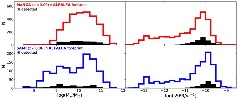
Figure 1: Top: Stellar mass and specific SFR distributions of galaxies that lie in the overlap sky region between MaNGA and ALFALFA surveys, restricted to the ALFALFA redshift interval ($z<0.06$). Filled histograms show the subsets with Hi detections from ALFALFA. Bottom: Same distributions for the SAMI Galaxy Survey, similarly restricted to ALFALFA footprint and redshift limits.

The past couple of decades have seen tremendous progress in our understanding of the physics of galaxies in the local Universe, thanks to the advent of 3D multiplexed large spectroscopic surveys in the optical and surveys of the cold interstellar medium at cm and mm wavelengths. The largest integral-field spectroscopy (IFS) surveys to date are the Sydney-AAO Multi-object Integral-field unit (SAMI, Bryant et al., 2015; Croom et al., 2021) Galaxy Survey and the Mapping Nearby Galaxies at Apache Point Observatory (MaNGA, Bundy et al., 2015) survey, which combined provided detailed stellar and emission line diagnostics for over 13,000 galaxies at redshift $z<0.15$. Radio surveys of the cold gas component have measured the global content of atomic (Hi) and molecular hydrogen (H₂, traced by carbon monoxide emission) for $\sim$50,000 and $\sim$1,000 galaxies at $z<0.06$ respectively, and mapped their kinematics and distributions down to the scales of giant molecular clouds, but only for small samples of very nearby galaxies (see Saintonge & Catinella 2022 and references therein).

The limited overlap currently present between cold gas and IFS samples prevents us from carrying out large statistical studies, which would allow us to characterize the physics of the gas-star formation cycle and quantify second-order trends that might drive the scatter of the main scaling relations. Even when we focus on untargeted Hi surveys, which provided the vast majority of global Hi measurements currently available, the overlap between Hi detections and IFS surveys is very limited (largely due to differences in sky footprints and median redshift distributions) and significantly biased towards the most gas-rich, star-forming systems. This is illustrated in Fig. 1, which shows the distributions of stellar mass and specific star-formation rate (SFR; specific $\rm SFR\equiv SFR/$$M_{\star}$) of MaNGA and SAMI, restricted to the sky footprint and redshift limit of the Arecibo Legacy Fast ALFA (ALFALFA; Giovanelli et al., 2005; Haynes et al., 2018) untargeted Hi survey. Even within the ALFALFA volume, only a small fraction of MaNGA and SAMI galaxies is detected in Hi by ALFALFA ($\sim$13% in both cases, filled histograms), and these are all star-forming systems (specific SFR $\gtrsim 10^{-11}$ $yr^{-1}$). This situation has motivated dedicated follow-up Hi observations of IFS samples, such as Hi-MaNGA (Masters et al., 2019; Stark et al., 2021) and SAMI-Hi, which is presented in this paper.

Increasing the number of galaxies with global Hi and IFS observations is a step in the right direction, but there remain important differences between these datasets in terms of spatial and spectral resolution, as well as field-of-views. Thus, these observations are highly complementary and can provide important insights into how galaxies form and evolve, by shedding light on the interplay between their cold gas reservoirs and their stellar and ionised gas components at different spatial scales. For instance, Hi rotation curves and $\rm H\alpha$ ones (obtained via Fabry-Perot, long-slit or IFS) have been combined to more accurately probe the galaxy gravitational potential for small samples (e.g., Noordermeer et al., 2007; Martinsson et al., 2013; Korsaga et al., 2019), but even the single velocity point provided by global Hi measurements can be useful to constrain the outer parts of rotation curves obtained from optical data (e.g., Cecil et al., 2016; Taranu et al., 2017). This synergy will become even more important when the next-generation Hi extragalactic surveys with the Square Kilometre Array (SKA; Carilli & Rawlings, 2004) and its pathfinder facilities (i.e., the Australian SKA Pathfinder, ASKAP: Johnston et al. 2008, Hotan et al. 2021; the Karoo Array Telescope, MeerKAT: Booth et al. 2009, Jonas & MeerKAT Team 2016, and the APERture Tile in Focus upgrade of the Westerbork Synthesis Radio Telescope, APERTIF: Verheijen et al. 2008) will deliver data for millions of galaxies, most of which will be spatially unresolved or marginally resolved. For instance, the Widefield ASKAP L-band Legacy All-sky Blind surveY (WALLABY; Koribalski et al. 2020) alone is expected to detect $\sim$210,000 galaxies out to $z\sim 0.1$ (Westmeier et al., 2022), whereas deeper Hi surveys such as DINGO (Deep Investigation of Neutral Gas Origins, Meyer 2009), MIGHTEE-HI (MeerKAT International GHz Tiered Extragalactic Exploration, Jarvis et al. 2016; Maddox et al. 2021) and especially LADUMA (Looking At the Distant Universe with the MeerKAT Array, Holwerda et al. 2012; Blyth et al. 2016), will detect (spatially unresolved) 21 cm emission from thousands of galaxies at higher redshifts.

With this in mind we carried out SAMI-Hi, a new Hi survey designed to increase the overlap between IFS and global Hi samples by targeting galaxies observed as part of the SAMI Galaxy Survey with the Arecibo radio telescope. Our goal is to provide the community with a sample that is representative of the star-forming main sequence population probed by SAMI to investigate how far we can push the combination of spatially unresolved Hi measurements and data from large IFS surveys. In this paper, we present the survey and Hi data release and compare dynamical scaling relations of local galaxies based on Hi velocity widths and $\rm H\alpha$ rotation curves. In a companion paper (Watts et al., 2022), we use SAMI-Hi to investigate how IFS data give us insights into the physical origin of kinematic asymmetries observed in Hi global spectra, and whether $\rm H\alpha$ and global Hi asymmetries are related.

One interesting area to explore with a sample with both IFS and Hi data available is that of kinematic scaling relations such as the Tully Fisher relation (TFR; Tully & Fisher, 1977). The TFR is a tight, empirical correlation between the luminosity or stellar mass and the rotational velocity of disk galaxies, reflecting the underlying link between the luminous and total (dynamical) mass of galaxies. The stellar TFR is known to break down at low stellar masses ($M_{\star}$$\lesssim 10^{9}$ M_⊙), as gas-rich dwarf galaxies scatter below the relation (i.e., they are under-massive for their rotational velocity; McGaugh et al. 2000). A more fundamental relation is the baryonic TFR, which is obtained by replacing the stellar mass with the total baryonic mass (i.e., the sum of stars and cold gas, Hi and molecular gas, H₂) and remains linear in the dwarf regime (e.g., McGaugh et al. 2000; Begum et al. 2008; but see Mancera Piña et al. 2019, 2020, who found a small number of Hi-rich, ultradiffuse galaxies that scatter at low circular velocities for their baryonic mass). As a result, this relation has received significant attention in the past two decades (e.g., Gurovich et al., 2004; McGaugh, 2005; Geha et al., 2006; Stark et al., 2009; Zaritsky et al., 2014; Bradford et al., 2016; Lelli et al., 2016b; Papastergis et al., 2016; Ponomareva et al., 2018; Lelli et al., 2019; Ponomareva et al., 2021). Naturally, the samples available for baryonic TFR studies are smaller, since these require both optical and Hi measurements, with the H₂ content being usually neglected (because the interstellar medium of nearby galaxies is typically dominated by the Hi component; e.g., Saintonge & Catinella 2022). Rotational velocities are measured from $\rm H\alpha$ or Hi emission using global spectra or rotation curves, or from stellar kinematics, and are often considered as proxies for circular velocities. While this is a good approximation for cold gas in most cases (as the contribution from asymmetric drift for Hi and CO is generally small compared to their rotational velocities, except at very small stellar masses), deriving circular velocities from stellar or $\rm H\alpha$ kinematics requires proper correction for asymmetric drift using velocity dispersion measurements (e.g., Cresci et al., 2009; Leung et al., 2018; Varidel et al., 2020).

The TFR has been studied for decades by the Hi and optical communities, initially for its value as a distance indicator and later for its importance for galaxy evolution studies (e.g., Aaronson et al., 1979; Bottinelli et al., 1983; Giovanelli et al., 1997b; Verheijen, 2001; Kannappan et al., 2002; Courteau et al., 2007; Pizagno et al., 2007; Reyes et al., 2011). More recently, IFS surveys (as well as molecular gas studies, e.g. Davis et al., 2011; Tiley et al., 2016; Topal et al., 2018) have contributed to the existing body of work (e.g., Cortese et al., 2014; Bloom et al., 2017; Aquino-Ortíz et al., 2018; Barat et al., 2019). Interestingly, optical studies based on both IFS and long-slit spectroscopy have found an increase of scatter of the stellar-mass TFR at low stellar masses (Simons et al., 2015; Bloom et al., 2017), which is not seen in the Hi relation (this scatter is in the opposite direction of the gas-rich dwarf galaxies that are outliers of the Hi stellar TFR, but not of the baryonic one). The scatter at low stellar mass of the optical TFR has been attributed to an increase of gas velocity dispersion (Simons et al., 2015), potentially associated with high $\rm H\alpha$ kinematic asymmetry (Bloom et al., 2017) in those systems.

Naturally, comparing Hi and optical and TFRs presents several challenges because, in addition to different sample selection, tensions could arise from the different kinematic tracers used (cold vs. ionised gas or stars), their radial extent, velocity definition (circular vs rotational) and the radius at which the velocity is measured (see, e.g., Courteau, 1997; Verheijen, 2001; Catinella et al., 2007; Lelli et al., 2019). Lelli et al. (2019) discussed some of these points in detail, and showed how these differences affect the baryonic TFR based on the Spitzer Photometry and Accurate Rotation Curve (SPARC; Lelli et al., 2016a) sample of galaxies with Hi and $\rm H\alpha$ rotation curves available. This is particularly important when comparing TFR samples based on local galaxies with higher redshift measurements (e.g., Fernández Lorenzo et al., 2009; Übler et al., 2017; Tiley et al., 2019) or predictions from theory and numerical simulations (e.g., Mo et al., 1998; Navarro & Steinmetz, 2000; Governato et al., 2007; Marinacci et al., 2014; Brook et al., 2016; Glowacki et al., 2020). In this context, here we compare the stellar and baryonic mass TFRs based on these tracers and discuss the origin of the tensions mentioned above for a sample with both $\rm H\alpha$ and Hi data available and uniformly measured.

This paper is organised as follows. In § 2 and § 3 we describe our sample selection and Arecibo observations. The kinematic measurements based on SAMI are summarised in § 4. In § 5, we characterise the SAMI-Hi sample and present our main results. We summarise and conclude in § 6, and present the Hi data release in Appendix. All the distance-dependent quantities in this work are computed assuming a cosmology with $H_{0}=70$ km s^-1 Mpc^-1, $\Omega_{m}=0.3$ and $\Omega_{\Lambda}=0.7$. We assume a Chabrier (2003) initial mass function. AB magnitudes are used throughout the paper.

2 Sample selection

Our sample is selected from the SAMI Galaxy Survey (Bryant et al., 2015; Croom et al., 2021), which includes 3068 galaxies with stellar masses greater than $\rm 10^{7}~{}M_{\odot}$ and redshifts $0.004<z<0.095$, observed with the Sydney-AAO Multi-object Integral field spectrograph (SAMI; Croom et al., 2012) on the 3.9-meter Anglo-Australian Telescope. The survey includes four volume-limited, stellar-mass selected galaxy samples extracted from the three equatorial fields of the Galaxy And Mass Assembly (GAMA; Driver et al., 2011) survey. Additional fields covering 8 clusters probe higher density environments. Each integral field unit (‘hexabundle’) covers a circular field of view of $\sim$14.9 arcsec in diameter. 13 hexabundles feed the SAMI spectrograph, which provides a spectral coverage of the 3650–5800 and 6240–7450 Å wavelength intervals with dispersions of 1.05 and 0.59 Å pixel^-1, respectively. Individual SAMI fibers have a diameter of $\sim$1.6 arcsec each.

SAMI-Hi is the combination of two dedicated Arecibo proposals (see § 3) and Hi detections from the ALFALFA survey. For our pilot proposal, we selected SAMI targets that had IFS data already available at the time of the observations (2015) and were easily observable from Arecibo (i.e. in the GAMA equatorial fields, with declinations $\delta\geq 1$^∘ and redshift $0.01<z<0.04$). For our second proposal, the sample selection was more clearly defined. Specifically, we started from the 1311 galaxies that had already been observed by SAMI in the GAMA regions in 2017. First, we imposed a declination ($0<\delta<37$^∘) and redshift ($z<0.04$) cut to make Arecibo observations more efficient and avoid radio frequency interference (RFI). Second, we added a low stellar mass cut of 10^8.6 M_⊙, to avoid objects whose $\rm H\alpha$ velocity dispersion may be below the SAMI resolution limit and focused on star-forming galaxies, defined as objects with specific SFR higher than 10^-11 $yr^{-1}$. Stellar masses are derived from the rest-frame $i$-band magnitude and $g-i$ colour as described in Bryant et al. (2015). Integrated SFRs are taken from Davies et al. (2016) and were obtained via spectral energy distribution fitting using the MAGPHYS code (da Cunha et al., 2008). Lastly, we removed galaxies with effective radius ($r_{e}$) smaller than 2.5 arcsec (i.e., for which the inner regions would not be resolved) or larger than 7.5 arcsec (i.e., for which the SAMI coverage does not reach more than 1 effective radius). Effective radii were estimated from single Sersic fit to the Sloan Digital Sky Survey (SDSS; York et al., 2000) $r$-band images as described in Kelvin et al. (2012). Excluding galaxies already detected by ALFALFA, this gave us a sample of 104 targets.

We obtained Hi emission-line spectra for 153 galaxies with these dedicated follow-up observations (78 from the first proposal and 75 from the second one). Together with 143 good-quality ALFALFA Hi detections (i.e., classified as “code 1”, with a typical signal-to-noise ratio SNR$\geq 6.5$), our sample includes 296 galaxies with IFS from SAMI and global Hi spectra from Arecibo.

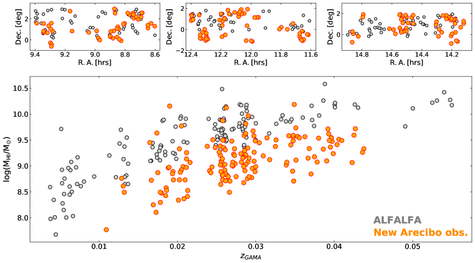
Figure 2: Sky distribution (top) and plot of the Hi mass as a function of optical spectroscopic redshift (bottom) for the galaxies in SAMI-Hi. Orange and gray circles indicate the new Arecibo observations and ALFALFA data, respectively (see text).

3 Arecibo observations and data reduction

SAMI-Hi observations were carried out with the Arecibo radio telescope between 2015 and 2017. These were scheduled in 125 observing runs under programs A2934 and A3116; the total telescope time allocation was 161 hours.

All the observations were carried out remotely except for one week in March 2017, when members of the Undergraduate ALFALFA Team observed on site. We used the standard position-switching mode, the L-band wide receiver and the interim correlator as a backend. Two correlator boards with 12.5 MHz bandwidth, one polarization, and 2048 channels per spectrum (yielding a velocity resolution of 1.4 km s^-1 at 1370 MHz before smoothing) were centered at or near the frequency corresponding to the GAMA redshift of the target. The Hi spectra were recorded every second with 9-level sampling. We observed each galaxy until detected, but moved to another target if there was no hint of Hi signal within the first 4-5 on-off pairs. On-source integration times ranged between 2 and 50 minutes per galaxy, with an average of 15 minutes. This is significantly deeper than ALFALFA, for which the integration time is $\sim$1 minute.

The data reduction, performed in the IDL environment, was the same as for the extended GALEX Arecibo SDSS Survey (xGASS; Catinella et al., 2018), and included Hanning smoothing, spectral bandpass subtraction, RFI excision, and flux calibration. Our RFI excision technique is illustrated in detail in Catinella & Cortese (2015). Briefly, the spectra obtained from each on/off pair are weighted by 1/$rms^{2}$, where $rms$ is the root mean square noise measured in the signal-free portion of the spectrum, and co-added. The two orthogonal linear polarizations (kept separated up to this point) are averaged to produce the final spectrum; polarization mismatch, if significant, is noted in Appendix B. The spectrum is then boxcar smoothed, spectral baseline subtracted and measured as explained in Catinella et al. (2010).

Observed velocity widths, $W_{50}$, are measured at the 50% level of each flux peak. We determine the peak flux density on both sides of the Hi profile and fit a straight line to each side (between the 15% and 85% levels of $f_{p}-rms$, where $f_{p}$ is the corresponding peak flux density). We identify the velocities $cz_{r}$, $cz_{a}$ corresponding to the 50% peak flux density (from the fits) on the receding and approaching sides, respectively, and define $W_{50}$ as the difference between these two velocities (and the Hi redshift as their average). This is the same algorithm used to measure Hi velocity widths for large Hi data sets such as Springob et al. 2005 (see their Section 3.2 for an illustration of this technique), ALFALFA (Haynes et al., 2018) and xGASS. The error on the observed velocity width is the sum in quadrature of the statistical and systematic uncertainties. Statistical errors depend primarily on the signal-to-noise of the Hi spectrum, and are obtained from the $rms$ noise of the linear fits to the edges of the Hi profile. Systematic errors depend on the subjective choice of the Hi signal boundaries (see Catinella et al., 2010), and are negligible for most of the galaxies in our sample (see also Appendix B).

Observed Hi widths are corrected for instrumental broadening and cosmological redshift as described in Catinella et al. (2012a). Hi rotational velocities are then computed by deprojecting the corrected half-widths to edge-on view:

$$V_{\rm HI}=\frac{W^{c}_{50}}{2\sin(i)},$$

where $i$ is the inclination to the line of sight. Inclinations are determined from the SDSS r-band axis ratio (b/a) as:

$$\cos(i)=\sqrt{\frac{(b/a)^{2}-q_{0}^{2}}{1-q_{0}^{2}}},$$

where $q_{0}$, the intrinsic axial ratio of a galaxy seen edge-on, is fixed at 0.2, appropriate for a thick disc (e.g., Guthrie, 1992; Giovanelli et al., 1997a; Weijmans et al., 2014; Tiley et al., 2019). We set the inclination to 90 degrees if $b/a<q_{0}$. The catalogues of Hi parameters and spectra for our SAMI-Hi observations are presented in Appendix A.

Lastly, we visually inspected the SDSS optical images of all the galaxies in our sample to determine which ones were affected by confusion within the Arecibo beam (full width half maximum size of $\sim$3.5 arcmin at 1.42 GHz). In these cases, two or more galaxies at very similar redshift lie within the radio beam, resulting in a blended signal from which we cannot reliably extract the Hi parameters of the target galaxy (in particular Hi flux and velocity width will be overestimated by an unknown amount). In total, we flagged 25 galaxies ($\sim$8% of the sample) for which confusion was certain, and identified these as systems with at least one late-type, similar size companion based on SDSS spectroscopy (i.e. with spectroscopic redshift available and within 0.002 of that of the target galaxy) within the beam. For our Arecibo observations, confusion is noted in Appendix B.

4 $\rm H\alpha$ velocity field measurements from SAMI

The extraction of $\rm H\alpha$ rotation curves from SAMI data and our procedure to measure $\rm H\alpha$ rotational velocities are described in detail in Tiley et al. (2019). Briefly, we start from the 2D line-of-sight emission line velocity maps obtained by fitting the LZIFU code (Ho et al., 2016) to the SAMI cubes (see Croom et al. 2021 for more details on the fitting procedure). Each SAMI velocity map is then centered on the peak of the continuum map, and the kinematic position angle is determined by using the maximum velocity gradient technique (i.e., by rotating the centred velocity map in 1-degree increments, and finding the value that maximizes the velocity gradient along a 3 pixel-wide horizontal slit). About 10% of these kinematic position angles were replaced after visual inspection. A rotation curve is then extracted from the velocity maps in a 3 pixel-wide slit along the major kinematic axis, by taking the weighted mean of the velocity values in pixel-wide steps within the slit.

We fit the SAMI $\rm H\alpha$ rotation curves with the commonly used arctangent model (Courteau, 1997), which is left free to shift along the radial and velocity axes within 1.5 arcsec and 200 km s^-1, respectively. $\rm H\alpha$ rotational velocities are measured from the best-fitting model at 1.3 $r_{\rm e}$ (sometimes requiring extrapolation, see § 5.2), where $r_{\rm e}$ is the effective (half-light) radius convolved to the seeing of the velocity map. This radius corresponds to 2.2 disk scale lengths, where the rotation curve of a pure exponential disk would peak (Freeman, 1970). Uncertainties on these velocities, which we refer to as $v_{2.2,obs}$, are obtained by bootstrap re-sampling the observed rotation curve and refitting 100 times. We also measured the maximum radial extent of the $\rm H\alpha$ emission along the kinematic axis, $R_{\rm max}$, and the corresponding observed and model velocity at this radius. Lastly, we correct the observed velocities for the effects of inclination and beam smearing using equation 6 in Tiley et al. (2019):

$$V^{\prime}_{\rm OPT}=\frac{\epsilon_{\rm R,PSF}}{\sin(i)}~{}v_{2.2,obs},$$

where $i$ is the inclination of the galaxy (see § 3) and $\epsilon_{\rm R,PSF}$ is a beam smearing correction factor that depends on the ratio of the galaxy size to the width of the seeing point spread function (PSF), and the rotation speed of the galaxy. To be consistent with Hi measurements, we also correct optical rotational velocities for cosmological redshift:

$$V_{\rm OPT}=V^{\prime}_{\rm OPT}/(1+z),$$

where $z$ is the redshift of the galaxy measured from its Hi spectrum.

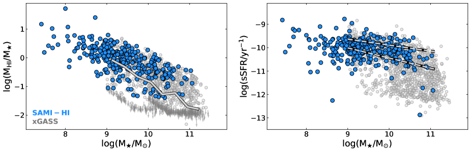
Figure 3: Left: Hi gas fraction versus stellar mass for SAMI-Hi (blue) and, for comparison, xGASS (gray circles: Hi detections; gray downward arrows: upper limits). The solid line indicates xGASS median gas fractions, computed including upper limits of non-detections. Right: specific SFR as a function of stellar mass for SAMI-Hi (blue) and xGASS (gray). Dashed lines enclose the xGASS star-forming sequence and correspond to $\pm 1\sigma$ deviation from the average.

5 Results

5.1 The SAMI-Hi sample

The sky distribution of the SAMI-Hi sample is shown on the top panels of Fig. 2, with orange and gray circles indicating the subsets with new Arecibo data and ALFALFA detections, respectively. The galaxies are roughly evenly distributed among the three equatorial GAMA fields centered at right ascensions of 9 hr (left), 12 hr (center) and 14.5 hr (right). The bottom panel shows the distribution of Hi mass as a function of optical spectroscopic redshift for the same subsets. As can be seen, our targeted Arecibo observations detected galaxies with Hi masses $\sim$1 dex smaller than ALFALFA at similar redshift. Unfortunately the $z>0.06$ redshift interval was not accessible due to RFI.

In order to better characterise the properties of SAMI-Hi, we compare it with xGASS, a reference sample of $\sim$1200 galaxies with homogeneously measured Hi and multi-wavelength parameters. Briefly, galaxies in xGASS were selected by redshift ($0.01\leq z\leq 0.05$) and stellar mass ($9\leq\log(M_{\star}/\rm M_{\odot})\leq 11.5$) only, forcing an approximately flat distribution in $M_{\star}$ (in each of the two volumes that make up the survey, i.e. $0.01\leq z\leq 0.02$ and $0.025\leq z\leq 0.05$) to increase statistics at the high $M_{\star}$ end. The targets were observed with Arecibo until detected, or until a gas fraction limit of a few per cent in gas mass fraction ($M_{\rm HI}$/$M_{\star}$) was reached, making these the most sensitive Hi observations of a large, representative sample to date. Fig. 3 compares SAMI-Hi (blue circles) and xGASS (gray symbols) on the gas fraction-stellar mass and specific SFR vs. stellar mass planes. On the left panel, small downward arrows are xGASS non-detections plotted at their 5$\sigma$ upper limits and the gray line shows the xGASS medians (computed including the upper limits; see Catinella et al. 2018). SAMI-Hi probes stellar masses almost 2 dex below xGASS, and does not reach quite the same high stellar masses as xGASS (this is because xGASS oversampled the high $M_{\star}$ regime), but where the two samples overlap, there is a clear offset. Specifically, SAMI-Hi galaxies have systematically higher gas fractions than xGASS at the same stellar mass, and are for the most part star-forming systems with specific SFRs above $\rm 10^{-11}~{}yr^{-1}$ (this is by selection, see § 2). For reference, the xGASS star-forming main sequence is indicated by the dashed lines on the right panel, which are at $\pm 1\sigma$ from the average relation (see Catinella et al. 2018 and Janowiecki et al. 2020 for details).

In what follows, we discard 27 galaxies from the SAMI-Hi sample: (a) 25 systems that are confused within the Arecibo beam (see § 3); (b) one galaxy with incorrect Hi parameters (SAMI 298862/AGC 243504, for which ALFALFA measured only one of the two Hi peaks, severely underestimating its velocity width); and (c) one galaxy with a measured $\rm H\alpha$ rotational velocity of 0 km s^-1 (SAMI 278684). Discarding these systems does not introduce significant biases (see Fig. 4). We refer to the resulting subset, which includes 269 galaxies, as the SAMI-Hi kinematic sample. As discussed in § 5.3, the pruned SAMI-Hi kinematic subset additionally excludes 56 galaxies with inclinations $i<40$^∘ and 12 systems with disturbed $\rm H\alpha$ kinematics (2 of which also have $i<40$^∘), thus including 203 galaxies.

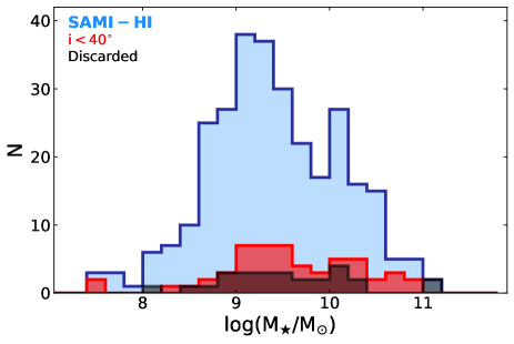
Figure 4: Stellar mass histograms showing the selection cuts applied to the sample. Blue: SAMI-Hi sample (N=296). Dark gray: galaxies that were discarded because of invalid $\rm H\alpha$ or Hi rotational velocities (N=27, see § 5.1). Red: low-inclination systems (N=56).

5.2 $\rm H\alpha$ and Hi rotational velocity comparison

Before presenting the TFRs for our sample in the next section, we compare the rotational velocities obtained from SAMI $\rm H\alpha$ rotation curves ($V_{\rm OPT}$, measured at 1.3 $r_{\rm e}$) and from Arecibo Hi global profiles ($V_{\rm HI}$, measured at 50% of the peaks). Fig. 5a shows the ratio between the two, $V_{\rm HI}$/$V_{\rm OPT}$, plotted as a function of stellar mass for the SAMI-Hi kinematic sample. While this velocity ratio does not depend on the galaxy’s inclination to the line-of-sight, we indicate low-inclination systems ($i<40$^∘) with empty symbols, as these are typically excluded in TFR studies. As expected from the fact that Hi measurements probe larger radii (and rotation curves are typically still rising at 1.3 $r_{\rm e}$), most galaxies have Hi rotational velocities that are larger than optical ones. The $V_{\rm HI}$/$V_{\rm OPT}$ ratio shows a clear dependence on stellar mass, in the sense that the lower $M_{\star}$ is, the more $V_{\rm OPT}$ underestimates $V_{\rm HI}$. This is quantified by the running medians (thick line); a linear fit to the gray points (not shown) has a correlation coefficient $r=-0.42$ and a scatter $\sigma=0.15$ dex. The reason for this trend with stellar mass is, again, due to a combination of rotation curve shapes and extent probed by the velocity tracers. When binned by galaxy luminosity and plotted as a function of normalised radius (e.g., galactocentric radius divided by scale length or optical radius), average rotation curve shapes vary smoothly, from slowly rising at low luminosity, to steeply rising in the central parts and then approximately flat in the brightest galaxies (e.g., Verheijen, 2001; Catinella et al., 2006). Thus, the ratio between rotational velocities measured in the outer parts and at 1.3 $r_{\rm e}$ increases at low stellar masses, where rotation curves are typically rising and have not reached the flat part. This implies systematic differences in the slopes of TFRs based on $\rm H\alpha$ and Hi measurements, as discussed in the next section.

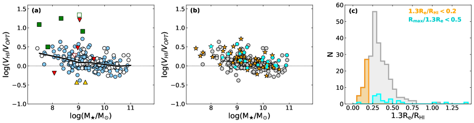
Figure 5: (a) Ratio of Hi-to-$\rm H\alpha$ rotational velocities (independent of inclination) versus stellar mass for the SAMI-Hi kinematic sample. Empty symbols indicate galaxies with low inclinations ($i<40$^∘), and colored symbols are problematic systems identified by visual inspection (green squares: mergers/messy; red downward triangles: outflows/counter-rotating; yellow triangles: wrong GAMA radii). The thick line shows the medians for the full sample. (b) Same as (a) but with problematic systems (squares and triangles) removed. Points here are colour-coded to highlight galaxies with $V_{\rm OPT}$ measured at a radius that is a small fraction of the Hi size (i.e., 1.3 $r_{\rm e}$/$R_{\rm HI}$$<0.2$; orange stars) and galaxies with the largest rotation curve extrapolations (i.e., $R_{\rm max}$/(1.3 $r_{\rm e}$) $<0.5$, where $R_{\rm max}$ is the extent of the rotation curve; cyan circles). (c) Distributions of 1.3 $r_{\rm e}$/$R_{\rm HI}$, i.e. the ratio of the radii where $V_{\rm OPT}$ and $V_{\rm HI}$ are measured (the size of the Hi disk is estimated from the Hi mass-size relation, see § 5.2) for the 3 subsets of galaxies shown in (b).

It is interesting to note that there are galaxies with Hi velocity widths that are smaller than optical ones. While at high stellar masses these galaxies are within the scatter of the relation, at lower masses ($\log(M_{\star}/\rm M_{\odot})\lesssim 9.5$) these are clearly outliers. We inspected the galaxies with $\log(V_{\rm HI}/V_{\rm OPT})<-0.1$ across the full $M_{\star}$ range, and concluded that these tend to be the low SNR tail of the Hi-detected population (about 80% are ALFALFA detections, half of which were detected with relatively low SNR of $6-8$). The strongest outliers, such as the two galaxies with $V_{\rm HI}$/$V_{\rm OPT}$$\sim$0.5 at $\log(M_{\star}/\rm M_{\odot})\sim 9$ (blue circles closest to the two yellow triangles), can be explained as having $V_{\rm HI}$ potentially underestimated. This illustrates some of the challenges involved in a detailed comparison between $\rm H\alpha$ and Hi velocity widths, even for reliable Hi detections. At the high stellar mass end, a few outliers can be explained by overestimated optical velocities, for instance due to large extrapolations in galaxies where the rotation curve traces a strong bar.

Fig. 5a also shows a few strong outliers above the relation. We visually inspected the SDSS images and SAMI velocity fields of several galaxies that were outliers of this relation and/or the TFRs presented below, and identified two systems with GAMA radii clearly wrong (yellow triangles in the figure) and nine with highly disturbed $\rm H\alpha$ velocity fields, due to mergers (green boxes) and presence of outflows or counter-rotation (downward red triangles). These galaxies are shown in Appendix C and should not be plotted on the TFR, as $V_{\rm OPT}$ is not a good measurement of rotational velocity.

The sample obtained after removing the systems marked with colored squares or triangles in Fig. 5a is shown in panel (b), without distinction by inclination. One might expect that the scatter of this relation could be in part related to the ratio of the radii where $V_{\rm OPT}$ and $V_{\rm HI}$ are measured, which could vary significantly from galaxy to galaxy. In order to test this hypothesis, we take advantage of the very tight Hi mass-size relation by Wang et al. (2016) to estimate the size of the Hi disk from the global Hi mass:

$$\log D_{\rm HI}=(0.506\pm 0.003)\log M_{\rm HI}-(3.293\pm 0.009),$$

where $D_{\rm HI}$ is the diameter in kpc of the Hi disk measured at a surface density $\Sigma_{\rm HI}=1~{}\rm M_{\odot}~{}pc^{-2}$. This relation holds over $\sim$5 dex in Hi mass and has a scatter of only $\sim$0.06 dex (see also Stevens et al., 2019).

The distribution of the 1.3 $r_{\rm e}$/$R_{\rm HI}$ ratio (where $R_{\rm HI}=0.5~{}D_{\rm HI}$) for this sample is presented in Fig. 5c, and indeed shows a significant variation, with four galaxies having estimated Hi radii that are shorter than 1.3 $r_{\rm e}$. Galaxies with 1.3 $r_{\rm e}$/$R_{\rm HI}$ ratio smaller than 0.2 (16% of the sample, orange histogram) do not appear to scatter more than the rest of the sample in panel (b), and are rather evenly distributed in stellar mass (orange stars).

Another factor that could contribute to the scatter of the velocity ratios is the extent of the $\rm H\alpha$ emission, $R_{\rm max}$, as rotation curves that do not reach 1.3 $r_{\rm e}$ require an extrapolation to estimate $V_{\rm OPT}$. Galaxies with the largest rotation curve extrapolations (i.e., for which $R_{\rm max}$/(1.3 $r_{\rm e}$) $<0.5$) are marked in cyan in panels (b) and (c). Comparing panels (a) and (b) it is interesting to note that, with the exception of a couple of galaxies, all the outliers above the relation in panel (b) are marked in cyan (largest rotation curve extrapolations) and/or orange (smallest 1.3 $r_{\rm e}$/$R_{\rm HI}$ ratios) and/or have low inclinations (empty circles in (a)).

As shown in Fig. 5, a small fraction of galaxies required significant extrapolation of their $\rm H\alpha$ rotation curves to measure $V_{\rm OPT}$ (9% of the sample, cyan symbols and histogram). For 49% of SAMI-Hi, rotation curves extend beyond 1.3 $r_{\rm e}$, therefore one might wonder if it would be preferable to measure $V_{\rm OPT}$ at $R_{\rm max}$ instead. While measuring rotational velocities at larger radii (where rotation curves are flatter) is better, it is equally important to determine these quantities in a consistent way (in this case, at the same relative position along the major axis of the disk) for the full sample, in order to avoid systematic effects that vary with rotation curve shape and extent (e.g., Catinella et al., 2007).

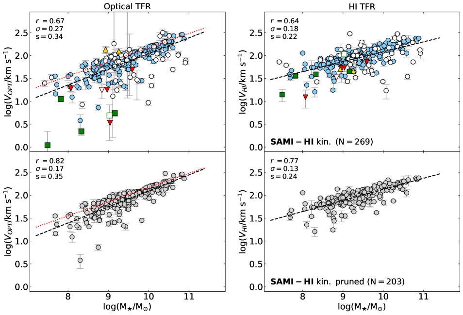
Figure 6: Top: optical (left) and Hi (right) stellar mass TFRs for the SAMI-Hi kinematic sample (same symbols as in Fig. 5a). Dashed lines are direct linear fits, with correlation coefficient, scatter and slope indicated on the top-left corners (see also Table 1). Bottom: TFRs for the kinematic, pruned sample, obtained by removing galaxies with inclination $i<40$^∘ and problematic systems (identified by squares and triangles in the top panels and in Fig. 5a). Red dotted lines on the left panels show the fit to a larger sample of SAMI galaxies from Bloom et al. (2017).

5.3 Stellar and baryonic mass Tully-Fisher relations

As typically done in optical studies, we present here TFRs by plotting rotational velocities as a function of stellar mass. This is in contrast to traditional TFR Hi studies, where luminosity or mass is treated as the dependent variable for distance indicator applications, and inverse fits are used to minimise the effect of Malmquist bias (e.g., Teerikorpi, 1984, 1997; Giovanelli et al., 1997b). Optical and Hi stellar mass TFRs based on the SAMI-Hi kinematic sample are compared in the top panels of Fig. 6, with the same symbols as in Fig. 5a. Error bars on the optical and Hi rotational velocities are computed as explained in § 4 and § 3, respectively, and do not include errors on the inclinations, which are dominated by the unknown uncertainty on the assumed intrinsic disc axial ratio. Dashed lines show direct fits to all the data (not including errors), with correlation coefficient, scatter and slope noted on the top-left corner of each panel (see also Table 1). In the top-left panel, a red dotted line indicates the fiducial fit to the TFR obtained by Bloom et al. (2017) for a sample of $\sim$700 SAMI galaxies, after excluding the low-mass (high kinematic asymmetry) outliers (their equation 4): $\log(V_{\rm rot}/$km s^-1) $=(0.31\pm 0.01)\log(M_{\star}/$M_⊙) $-0.93\pm 0.10$. If we excluded the low-mass outliers below the TFR from our fit as they did, we would obtain a result more consistent with Bloom et al. (2017). Unsurprisingly, both $\rm H\alpha$ and Hi TFRs have significant scatter ($\sim$0.3 and 0.2 dex, respectively), as our sample was not designed to obtain the tightest TFR, as done for example for distance indicator applications. Galaxies that are typically excluded from TFR studies include low-inclination systems (i.e., $i<40$^∘, indicated by empty symbols in the top panels), for which the deprojection to line-of-sight rotational velocity is particularly uncertain. Galaxies with complex $\rm H\alpha$ kinematics, for which $V_{\rm OPT}$ is not a reliable measure of rotational velocity (green and red symbols), are preferentially found at low stellar masses and are amongst the strongest outliers of the optical TFR, whereas they do not deviate significantly on the Hi TFR.

The bottom two panels of Fig. 6 show the pruned versions of the two TFRs, after removing galaxies with $i<40$^∘ (empty symbols) and/or with disturbed $\rm H\alpha$ kinematics (colored squares ans triangles). The subset of galaxies with low inclinations includes 13 galaxies with inclinations that were largely overestimated, typically due to the presence of a strong bar; these were identified by visually inspecting the SDSS images of all the remaining outliers after the first pruning, and are all galaxies with $M_{\star}$$>10^{9}$ M_⊙ that would have been excluded by our $i<40$^∘ cut (see Appendix C for more details).

Table 1: Fits to the stellar and baryonic TFRs presented in Fig. 6 (top four rows) and Fig. 8 (bottom two rows). We fit the linear relation $\log(V/$km s^-1) $=s\log(M/$M_⊙) + $q$, where $V$ is $V_{\rm OPT}$ or $V_{\rm HI}$ for the optical or Hi relations, and $M$ is $M_{\star}$ or $M_{\rm bar}$ for stellar or baryonic TFRs, respectively. The scatter $\sigma$ in $\log(V/$km s^-1) and the size of the sample are listed in the last two columns.

Relation	$s$	$q$	$\sigma$	N
OPT TFR	0.34 $\pm$ 0.03	$-$1.39 $\pm$ 0.27	0.27	269
Hi TFR	0.22 $\pm$ 0.02	$-$0.09 $\pm$ 0.17	0.18	269
OPT TFR, pruned	0.35 $\pm$ 0.02	$-$1.41 $\pm$ 0.18	0.17	203
Hi TFR, pruned	0.24 $\pm$ 0.01	$-$0.29 $\pm$ 0.14	0.13	203
OPT BTFR, pruned	0.44 $\pm$ 0.02	$-$2.43 $\pm$ 0.24	0.17	203
Hi BTFR, pruned	0.32 $\pm$ 0.02	$-$1.17 $\pm$ 0.17	0.13	203

While both $\rm H\alpha$ and Hi relations have tightened (by $\sim$0.1 and 0.05 dex, respectively) compared to the versions in the top panels, the $\rm H\alpha$ TFR (left) shows a number of outliers at low stellar mass ($M_{\star}$$\lesssim 10^{9.5}$ M_⊙) that are not seen in the Hi TFR (right). In Hi TFR studies it is well known that dwarf galaxies ($M_{\star}$$\lesssim 10^{9}$ M_⊙) systematically deviate from the main relation defined by larger systems, in the sense that, at fixed rotational velocity (i.e., dynamical mass), their stellar masses are smaller than expected. This is interpreted as due to the fact that a larger fraction of the baryonic mass (i.e., the sum of stellar and cold gas mass) in dwarf galaxies is in the form of cold gas, and indeed a tight and linear TFR is recovered when baryonic mass is plotted instead of stellar mass (McGaugh et al., 2000). Interestingly, the low $M_{\star}$ outliers of the $\rm H\alpha$ TFR scatter in the opposite direction: at fixed rotational velocity, stellar masses are higher than expected based on the fit to the larger systems.

As mentioned in the introduction, the increased scatter at low stellar mass of the optical TFR has been attributed to an increased importance of the velocity dispersion $\sigma$ in those systems (i.e., a decrease of $V_{\rm rot}/\sigma$; Simons et al. 2015; Bloom et al. 2017). In other words, a non-negligible part of the dynamical support in low-mass galaxies comes from random motions, not captured by $V_{\rm OPT}$. While this might be the case, other explanations are also possible. IFS samples such as SAMI cover only the inner parts of the galaxies, and velocities estimated at a fixed radius (generally within 2 effective radii) might systematically underestimate the rotational velocity of galaxies compared to global Hi measurements, which probe larger radii. This is especially true at low stellar masses, where rotation curves are typically rising and have not reached the flat part (e.g., Verheijen, 2001; Catinella et al., 2006). This is indeed demonstrated in Fig. 7, where we color-coded the SAMI-Hi (pruned) optical TFR by the ratio of Hi and $\rm H\alpha$ rotational velocities – the low-mass outliers of the relation are the galaxies for which $V_{\rm OPT}$ underestimates $V_{\rm HI}$ the most (although the opposite is not true – not all the systems with large $V_{\rm HI}$/$V_{\rm OPT}$ ratios are outliers).

Interestingly, while long-slit spectroscopy observations do not have the same aperture limitation as IFS, they too are likely to underestimate the rotational velocity, as a result of any alignment error between the photometric and the kinematic position angles (the latter being unknown a-priori). Either way, optical spectroscopy of faint galaxies is challenging and more prone to measurement errors. This is not necessarily the case with Hi observations – low mass galaxies are more gas rich (per unit of stellar mass, see Fig. 3) and have smaller velocity widths, making them easier to detect above the noise (compared to a galaxy with a the same Hi mass and larger stellar mass). We discuss below whether the low-mass outliers of the optical TFR have a physical explanation or are the result of measurements issues (errors or aperture effects).

Fig. 6 also shows that the slopes of the two TFRs are different, with the Hi relation being shallower (in this optical TFR representation, where $M_{\star}$ is the independent variable). This is caused by the combination of rotation curve shapes and rotational velocity definition, as discussed in the previous section.

For completeness, we show in Fig. 8 the $\rm H\alpha$ and Hi baryonic TFRs for the SAMI-Hi kinematic, pruned sample. Baryonic masses are estimated as $M_{\rm bar}=M_{\star}\ +1.36M_{\rm HI}$, where the factor 1.36 takes the contribution of Helium into account. Overlaid on both plots is the relation obtained by Lelli et al. (2019, see their Table 1) using optical rotational velocities measured at 2.2 disk scale lengths: $\log(M_{bar}/$M_⊙$)=(3.06\pm 0.08)\log(V_{2.2}/$km s^-1) $+3.75\pm 0.17$, which is indistinguishable from our own fit to the Hi relation. Compared to the stellar TFRs, the baryonic TFRs are steeper but the scatters are unchanged. The increased slopes are simply a consequence of the fact that Hi gas fractions are higher at lower stellar masses (e.g., Catinella et al., 2018; Saintonge & Catinella, 2022), thus lower $M_{\star}$ points shift rightwards by a larger amount. Most importantly, the optical baryonic TFR still has low $V_{\rm OPT}$ outliers that are not seen in the Hi relation.

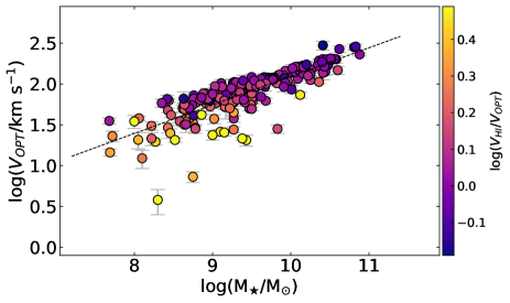
Figure 7: Optical stellar mass TFR of the SAMI-Hi kinematic, pruned sample and direct linear fit, reproduced from the bottom left panel of Fig. 6, with points color-coded by the logarithmic ratio of Hi-to-$\rm H\alpha$ rotational velocities.

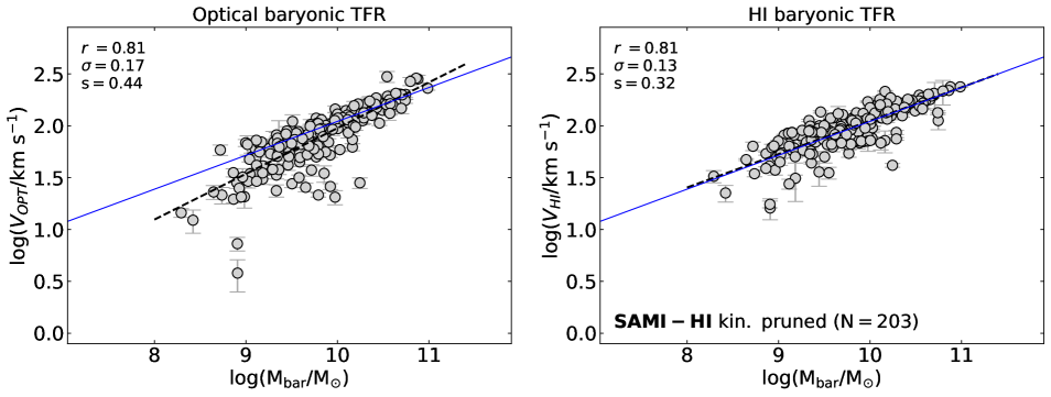
Figure 8: Optical (left) and Hi (right) baryonic mass TFRs for the SAMI-Hi kinematic, pruned sample. Dashed lines in each panel are direct linear fits, with correlation coefficient, scatter and slope indicated on the top-left corners (see also Table 1). Blue solid lines indicate the relation from Lelli et al. (2019).

6 Discussion and conclusions

In this paper we presented SAMI-Hi, an Arecibo program that measured global Hi parameters for 296 galaxies selected from the SAMI Galaxy Survey. In addition to releasing the new Hi data, we used this sample to illustrate the power, but also the challenges, of combining 3D optical data from large multiplexed IFS surveys with 21 cm single-dish observations to better understand dynamical scaling relations in the local Universe. While comparing IFS with spatially-resolved Hi data would be a more insightful exercise, the vast majority of the galaxies that will be detected by the next-generation Hi-line surveys with the SKA and its pathfinders will be spatially unresolved or only marginally resolved. (e.g., Saintonge & Catinella, 2022). Thus, our analysis is illustrative of what will be typically feasible once large Hi programs like WALLABY, DINGO and LADUMA enter full survey mode.

Our comparison of Hi and $\rm H\alpha$ rotational velocities builds on previous work (e.g., Courteau, 1997; Catinella et al., 2007; Lelli et al., 2019) and confirms how these estimates strongly depend on the tracer used and on the radial position at which the velocities are measured. Systematic differences between $V_{\rm OPT}$ measured at 1.3 effective radii from IFS observations and $V_{\rm HI}$ (which is closer to the maximum rotational velocity of galaxies) automatically lead to differences in slopes (and zero points) of dynamical scaling relations such as the TFR. While this has been noted in the past, for instance in comparisons between dynamical scaling relations obtained from Hi widths and optical long-slit spectroscopy, our analysis reframes the issue in the context of large IFS datasets and upcoming SKA-era Hi surveys and shows how a quantitative comparison of dynamic scaling relations obtained from these samples is far from trivial. Naturally, this applies not only to TFR analyses in the local Universe, but also to studies of the shape and cosmic evolution of other dynamical scaling relations (such as the mass-specific angular momentum relation; e.g., Fall, 1983; Romanowsky & Fall, 2012; Cortese et al., 2016; Tiley et al., 2021; Hardwick et al., 2022) and to comparisons with numerical simulations. Taking also into account how notoriously challenging it is to determine homogeneous velocity widths as a function of redshift even from the same data (Tiley et al., 2019), it is clear that extreme care must be taken in order to interpret offsets and differences in dynamical scaling relations based on different tracers and/or data sets. Therefore, when it comes to evolution of scaling relations with cosmic time, our results suggest that we should avoid using different tracers for different populations of galaxies, and primarily focus on homogenising observations of the same tracer (either Hi, $\rm H\alpha$ or other emission lines) across redshift, if possible.

On a more positive note, the analysis of our SAMI-Hi sample with both IFS and Hi data has provided us with some additional insights into the increase of scatter of the $\rm H\alpha$ TFR at low stellar masses claimed in previous works (Simons et al., 2015; Bloom et al., 2017). As shown in Fig. 6, when $\rm H\alpha$ rotational velocities are measured at 1.3 $r_{\rm e}$, the optical TFR has larger scatter than the Hi one, and this difference is more prominent at lower stellar masses (i.e., $M_{\star}$$\lesssim 10^{9.5}$ M_⊙), although this scatter increase seems less dramatic than what is reported by other groups. Most importantly, our inspection of the SAMI 2D velocity maps revealed that most of the significant low-mass outliers of the $\rm H\alpha$ TFR are not regular rotators but kinematically disturbed systems, either merger remnants or tidally perturbed (see Fig. A4). Interestingly, from optical imaging these galaxies appear to be unperturbed dwarf irregulars, and thus were not flagged as potentially confused within the radio beam (and excluded from the analysis).

Our findings support the conclusions of Simons et al. (2015) and Bloom et al. (2017), who pinned the increased scatter of the SAMI TFR at low stellar masses on the outliers with higher kinematic asymmetries compared to galaxies on the main relation. However, our view is that these systems should not be included in a TFR sample, because $\rm H\alpha$ widths measured from highly disturbed velocity fields should not be blindly interpreted as reliable estimates of rotational velocities. This becomes even more challenging with $\rm H\alpha$ velocity widths measured from long-slit spectroscopy, as the loss of spatial information compared to IFS data makes it harder to judge the degree of disturbance in the velocity field. This issue, combined with the fact that dwarf galaxies have intrinsically small rotational velocities at 1.3 $r_{\rm e}$ (comparable or even smaller than the $\rm H\alpha$ gas velocity dispersion), raises the question of how meaningful is to look at the stellar TFR at low stellar masses, where rotational velocity estimates are highly uncertain and encompass a tiny fraction of the total dynamical mass of the galaxies. As shown by various works (e.g., Kassin et al., 2007; Cortese et al., 2014; Barat et al., 2019; Barat et al., 2020; Aquino-Ortíz et al., 2018; Lelli et al., 2019), in this regime it is preferable to investigate dynamical scaling relations expressed in terms of circular velocity or S₀₅ parameter (which includes contributions from both rotational velocity and velocity dispersion), for which no increase in scatter at low masses has been confirmed so far.

In conclusion, below $M_{\star}$$\sim$10⁹ M_⊙ dynamical scaling relations are best investigated with Hi velocity widths. This is especially true for the TFR because, at those stellar masses, galaxies are Hi-dominated and the baryonic (rather than stellar) TFR is a more physical relation (McGaugh et al., 2000). Optical IFS observations are catching up but, in order to minimise limitations of current data sets, it is paramount to trace the rotation curves beyond 1.3 $r_{\rm e}$ and, ideally, with spectral resolutions significantly higher those of surveys like SAMI and closer to the typical values of Hi observations.

Data availability

The SAMI data cubes and value-added products used in this paper are available from Astronomical Optics’ Data Central service at https://datacentral.org.au/. Hi and optical parameters for the SAMI-Hi sample will also be available on Data Central, along with digital spectra of our Hi observations, once the paper is published on MNRAS.

Appendix A: Data Release

We present here SDSS postage stamp images, Hi-line spectra and catalog of Hi parameters for the 153 SAMI-Hi galaxies observed by our Arecibo programs. The content of the table is described below; notes on individual objects (marked with an asterisk in the second-last column of Table A1) are reported in Appendix B.

Hi source catalog.
This data release includes 153 detections. The measured Hi parameters for the detected galaxies are listed in Table A1, ordered by increasing right ascension:

Cols. 1 and 2: SAMI and SDSS identifiers.

Col. 3: GAMA spectroscopic redshift, $z_{\rm spec}$.

Col. 4: on-source integration time of the Arecibo observation, $T_{\rm on}$, in minutes. This number refers to on scans that were actually combined, and does not account for possible losses due to RFI excision (usually negligible).

Col. 5: velocity resolution of the final, smoothed spectrum in km s^-1. In general, lower signal-to-noise detections require more smoothing in order to better identify the edges and peaks of the Hi profiles, needed to measure the Hi parameters.

Col. 6: redshift, $z$, measured from the Hi spectrum. The error on the corresponding heliocentric velocity, $cz$, is half the error on the width, tabulated in the following column.

Col. 7: observed velocity width of the source line profile in km s^-1, $W_{50}$, measured at the 50% level of each peak (see § 3). The error on the width is the sum in quadrature of the statistical and systematic uncertainties in km s^-1. Systematic errors depend on the subjective choice of the Hi signal boundaries and are negligible for most of the galaxies in our sample (see also Appendix B).

Col. 8: velocity width corrected for instrumental broadening and cosmological redshift only, $W_{50}^{c}$, in km s^-1 (see Catinella et al. 2012b for details). No inclination or turbulent motion corrections are applied.

Col. 9: integrated Hi-line flux density in Jy km s^-1, $F_{\rm HI}\equiv\int S~{}dv$, measured on the smoothed and baseline-subtracted spectrum (observed velocity frame). The reported uncertainty is the sum in quadrature of the statistical and systematic errors (see col. 7). The statistical errors are calculated according to equation 2 of S05 (which includes the contribution from uncertainties in the baseline fit).

Col. 10: rms noise of the observation in mJy, measured on the signal- and RFI-free portion of the smoothed spectrum.

Col. 11: signal-to-noise ratio of the Hi spectrum, S/N, estimated following Saintonge (2007) and adapted to the velocity resolution of the spectrum. This is the definition of S/N adopted by ALFALFA, which accounts for the fact that for the same peak flux a broader spectrum has more signal.

Col. 12: base-10 logarithm of the Hi mass, $M_{\rm HI}$, in solar units, computed via:

$$\frac{M_{\rm HI}}{\rm M_{\odot}}=\frac{2.356\times 10^{5}}{(1+z)^{2}}\left[\frac{d_{\rm L}(z)}{\rm Mpc}\right]^{2}\left(\frac{\int S~{}dv}{\rm Jy~{}km~{}s^{-1}}\right)$$ (1)

where $d_{\rm L}(z)$ is the luminosity distance to the galaxy at redshift $z$ as measured from the Hi spectrum in the observed velocity frame.

Col. 13: base-10 logarithm of the Hi mass fraction, $M_{\rm HI}$/$M_{\star}$.

Col. 14: quality flag, Q (1=good, 2=marginal and 5=confused). An asterisk indicates the presence of a note for the source in Appendix B. Code 1 indicates reliable detections, with a S/N ratio of order of 6.5 or higher. Marginal detections have lower S/N magenta(between 5 and 6.5), thus more uncertain Hi parameters, but are still secure detections, with Hi redshift consistent with the SDSS one. We flag galaxies as “confused” when most of the Hi emission is believed to originate from another source within the Arecibo beam. For some of the galaxies, the presence of small companions within the beam might contaminate (but is unlikely to dominate) the Hi signal – this is just noted in Appendix B.

Col. 15: Arecibo project code.

SDSS postage stamps and Hi spectra.
Figure A1 shows SDSS images and Arecibo Hi spectra for a the first 10 galaxies included in this data release. The galaxies in each figure are ordered by increasing SAMI number, indicated on the top right corner of each spectrum. The SDSS images show a 1 arcmin square field, i.e. only the central part of the region sampled by the Arecibo beam (the half power full width of the beam is $\sim$3.5′ at the frequencies of our observations). Therefore, companions that might be detected in our spectra typically are not visible in the postage stamps, but they are noted in Appendix B. The Hi spectra are always displayed over a 3000 km s^-1 velocity interval, which includes the full 12.5 MHz bandwidth adopted for our observations. The Hi-line profiles are calibrated, smoothed (to a velocity resolution between 5 and 15 km s^-1, as listed in Table A1), and baseline-subtracted. A red, dotted line indicates the heliocentric velocity corresponding to the optical spectroscopic redshift from GAMA. The shaded area and two vertical dashes show the part of the profile that was integrated to measure the Hi flux and the peaks used for width measurement, respectively.

Table A1: Hi Properties of SAMI-HI detections

			$T_{\rm on}$	$\Delta v$		$W_{50}$	$W_{50}$c	$F$	rms		log $M_{\rm HI}$
SAMI	SDSS ID	$z_{\rm spec}$	(min)	(km s-1)	$z$	(km s-1)	(km s-1)	(Jy km s-1)	(mJy)	S/N	(M⊙)	log $M_{\rm HI}$/$M_{\star}$	Q	Proj
(1)	(2)	(3)	(4)	(5)	(6)	(7)	(8)	(9)	(10)	(11)	(12)	(13)	(14)	(15)
375402	J083606.39+011823.0	0.0129	10	12	0.013166	112$\pm$ 7	104	0.77$\pm$ 0.05	0.53	28.1	8.76	0.33	1*	a2934
322910	J083734.87+013426.0	0.0309	10	7	0.030971	51$\pm$ 2	46	0.38$\pm$ 0.03	0.73	19.1	9.19	-0.55	1	a2934
300477	J083849.62+010715.6	0.0291	15	13	0.029127	172$\pm$ 2	161	0.39$\pm$ 0.05	0.49	12.2	9.15	-0.10	1	a2934
375531	J083850.61+012418.0	0.0290	9	13	0.029117	148$\pm$ 18	137	2.57$\pm$ 0.07	0.73	58.2	9.97	0.52	5*	a3116
422289	J084106.54+023436.0	0.0318	30	13	0.031422	204$\pm$ 8	192	0.31$\pm$ 0.04	0.35	12.4	9.12	-0.44	5*	a3116
422320	J084114.60+023503.6	0.0314	8	13	0.031408	223$\pm$ 2	210	0.83$\pm$ 0.09	0.70	15.8	9.54	-0.02	1*	a2934
417392	J084134.33+021119.8	0.0287	18	13	0.028710	192$\pm$ 4	181	0.30$\pm$ 0.04	0.38	11.5	9.03	0.15	1	a2934
345682	J084242.49+015707.0	0.0255	10	12	0.025421	198$\pm$ 4	187	0.88$\pm$ 0.07	0.62	20.4	9.39	0.11	1*	a2934
417424	J084333.16+021239.7	0.0299	8	13	0.029897	242$\pm$ 5	228	0.80$\pm$ 0.08	0.62	16.7	9.48	0.18	1	a2934
345754	J084428.45+020350.2	0.0256	35	12	0.025518	261$\pm$ 17	248	0.28$\pm$ 0.05	0.37	9.5	8.89	-1.36	1	a3116
517167	J084438.72+022439.5	0.0299	19	13	0.029864	159$\pm$ 7	148	0.20$\pm$ 0.04	0.40	8.2	8.89	-0.35	1*	a3116
422486	J084443.28+023421.8	0.0261	20	10	0.026115	52$\pm$ 5	46	0.18$\pm$ 0.03	0.48	11.5	8.71	-0.07	1*	a3116
517249	J084612.24+022437.7	0.0281	8	13	0.028073	119$\pm$ 7	110	0.51$\pm$ 0.06	0.64	14.7	9.24	-0.16	1*	a3116
517302	J084654.29+023336.2	0.0287	10	13	0.028983	368$\pm$ 20	351	1.81$\pm$ 0.10	0.59	31.9	9.81	-0.37	5*	a2934
323507	J084808.41+013357.7	0.0399	25	13	0.039824	187$\pm$ 1	173	0.26$\pm$ 0.05	0.41	9.1	9.24	-0.20	1	a3116

Note. – The full version of this table is available online.

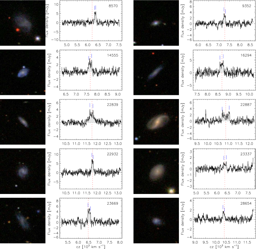
Figure A1: SDSS postage stamp images (1 arcmin square) and Hi-line profiles of SAMI-Hi galaxies, ordered by increasing SAMI number (indicated in each spectrum). The Hi spectra are calibrated, smoothed and baseline-subtracted. A dotted line and two dashes indicate the heliocentric velocity corresponding to the GAMA optical redshift and the two peaks used for width measurement, respectively. This is a sample of the complete figure, which is available in the online version of the article.

Appendix B: Notes on Individual Objects

We list here notes for galaxies marked with an asterisk in the second-last column of Table A1. The galaxies are ordered by increasing SAMI number. In what follows, AA2 is the abbreviation for ALFALFA detection code 2.

14555 – AA2; galaxy $\sim$3.5 arcmin SE has z=0.114.
22839 – blend emission from galaxy group, including large blue galaxy $\sim$2.5 arcmin SE (SDSS J115705.93+010732.1, $z=0.039517$), blue gal. $\sim$2 arcmin S (SDSS J115657.00+010657.0, $z=0.0393$) and small galaxy $\sim$3 arcmin S (SDSS J115654.22+010557.3, $z=0.039458$); edge-on disk $\sim$2.5 arcmin NE has $z=0.049$.
22887 – RFI spike at 1375 MHz ($\sim$9900 km s^-1); small galaxy $\sim$2 arcmin E has $z=0.079$.
22932 – AA2; disk galaxy $\sim$2.5 arcmin S has $z=0.064$.
23337 – galaxy $\sim$1 arcmin N has $z=0.078$; blue galaxy $\sim$3 arcmin SE has $z=0.066$.
23669 – RFI spike at 1392 MHz ($\sim$6150 km s^-1) visible in final spectrum; companion $\sim$2 arcmin S, SDSS J121035.31+010143.4 ($z=0.020115$, 6030 km s^-1) not detected. AA2.
28860 – blend with giant face-on spiral $\sim$3 arcmin SW, SDSS J142720.36+010133.1 (UGC 9254, $z=0.02569$, 7702 km s^-1).
30377 – high-frequency edge uncertain, systematic error.
31452 – small blue smudge $\sim$50 arcsec W without optical redshift, unlikely to significantly contaminate the signal; two blue galaxies within 4 arcmin in background ($z>0.06$).
31509 – RFI spike near 1382.5 MHz ($\sim$8300 km s^-1).
31620 – two background galaxies (small blue galaxy $\sim$30 arcsec S, SDSS J120155.54-010445.4, $z=0.117$ and small galaxy $\sim$3 arcmin NW, $z>0.11$); narrow RFI spike at 1392 MHz (within profile) not visible in spectrum.
40765 – low-frequency edge uncertain, systematic error.
41164 – RFI spike near 1392.5 MHz ($\sim$6100 km s^-1).
56064 – blue galaxy $\sim$2.5 arcmin NE has $z=0.071$.
69740 – AA2; galaxy $\sim$2.5 arcmin E has $z=0.058$.
69844 – blue fuzzy galaxy $\sim$10 arcsec W, no optical redshift.
69864 – galaxy $\sim$30 arcsec E has $z=0.095$.
71382 – RFI spike at 1388.8 MHz ($\sim$6800 km s^-1); small blue galaxy $\sim$1 arcmin SW has $z=0.073$.
77373 – two galaxies $\sim$2 arcmin N have $z=0.15$.
79771 – small face-on galaxy $\sim$30 arcsec NW, no optical redshift.
84048 – RFI spike near 1388.8 MHz ($\sim$6800 km s^-1).
91926 – polarization mismatch; two background galaxies (blue spiral $\sim$2 arcmin S, SDSS J141701.67+002837.4, $z=0.053$ and early-type $\sim$2.5 arcmin NE, SDSS J141712.85+003159.7, $z=0.077$).
92770 – galaxy $\sim$3 arcmin SW has $z=0.136$; galaxy $\sim$2.5 arcmin N has $z=0.118$.
93167 – AA2.
99393 – detected blue companion $\sim$2 arcmin N, SDSS J121037.24+010353.7 ($z=0.021841$, $cz=6548$ km s^-1).
99511 – blue galaxy $\sim$2.5 arcmin N has $z=0.083$.
100192 – high-frequency edge uncertain, systematic error.
105600 – confused/blend with edge-on disk $\sim$3 arcmin E, SDSS J141057.69+010208.6 ($z=0.025407$, 7617 km s^-1); large vel offset suggests that this might be just one side of the Hi profile of the large companion.
106049 – polarization mismatch.
209279 – AA2.
209708 – polarization mismatch.
209743 – blue cloud $\sim$40 arcsec NE without optical redshift, possibly contaminating signal.
220275 – polarization mismatch; AA2. Detected galaxy in OFF, SDSS J120842.76+012722.8 ($z=0.018547$, 5560 km s^-1).
220371 – AA2.
220578 – early-type galaxy $\sim$1 arcmin W has $z=0.129$ (NED); two other galaxies $\sim$1.5 arcmin NW, one has $z=0.130$, the other has no optical redshift, but likely in background.
220750 – blue galaxy $\sim$20 arcsec NE, no optical redshift, possibly confused.
227673 – AA2.
228432 – blue galaxy $\sim$1 arcmin S, SDSS J142933.33+010616.0, possibly contaminating signal (no redshift in SDSS, NED has z=0.029490 from FoF??)
230560 – galaxy $\sim$2.5 arcmin SW has $z=0.078$.
230714 – two large galaxies $\sim$4 arcmin SE and $\sim$4 SW in foreground ($z=0.016$ and 0.019, respectively).
239490 – AA2.
251297 – AA2.
251367 – blend with two blue galaxies: SDSS J143255.33+015209.0, $\sim$2 arcmin S ($z=0.030023$, 9001 km s^-1) and SDSS J143245.52+015238.8 $\sim$2.5 arcmin W ($z=0.029892$, 8961 km s^-1).
273951 – blend with large galaxy 1 arcmin NW, SDSS J122339.84+011925.5 ($z=0.026436$, 7925 km s^-1); RFI spike at 1388.8 MHz ($\sim$6800 km/s).
273952 – blue galaxy $\sim$4 arcmin SW, SDSS J122339.84+011925.5 ($z=0.026436$, 7925 km s^-1), partly detected?
278684 – polarization mismatch.
278741 – AA2; large spiral $\sim$3 arcmin S, SDSS J085339.27+004529.4 ($z=0.04116$, 12339 km s^-1), not detected.
289116 – 4 foreground galaxies within 4 arcmin ($z>0.022$).
289429 – galaxy $\sim$3 arcmin W and $\sim$3 arcmin E in background ($z>0.11$).
296685 – notice large edge-on disk $\sim$3 arcmin NW, SDSS J141110.08+012828.9, at the same redshift; however the Hi signal is so narrow that contamination is very unlikely.
296847 – blend with blue companion $\sim$1 arcmin S, SDSS J141411.10+013006.4 (GAMA 296848 below). AA2.
296848 – blend with blue companion $\sim$1 arcmin N, SDSS J141409.31+013111.2, $z=0.025927$ (GAMA 296847 above).
301201 – AA2.
302846 – blue disk $\sim$4 arcmin NE, SDSS J091843.59+012341.0, has $z=0.037$.
320068 – blue gal. $\sim$2 arcmin NE has $z=0.025$; early type $\sim$1.5 arcmin SE has $z=0.100$.
320281 – blend with large blue galaxy $\sim$2.5 arcsec NE, SDSS J143042.33+015253.2 ($z=0.033899$, 10163 km s^-1); small blue galaxy $\sim$1 arcmin N has $z=0.099$.
345682 – notice blue blob $\sim$1.5 arcmin SE, SDSS J084245.27+015550.6 (no optical redshift).
375531 – blend with blue galaxy $\sim$30 arcsec SE, SDSS J083852.35+012356.8 ($cz=8776$ km s^-1 from NED, CGCG 004-098).
375402 – large galaxy $\sim$1.5 arcmin NW, SDSS J083603.33+011947.1, no optical redshift.
422289 – confused/blend with large disk galaxy $\sim$2 arcmin E, SDSS J084114.59+023503.6 ($z=0.031423$, 9420 km s^-1).
422320 – AA2.
422486 – RFI spike at 1388.8 MHz ($\sim$6800 km s^-1).
517167 – galaxy $\sim$1 arcmin E has $z=0.077$.
517249 – AA2.
517302 – blend with blue companion $\sim$1 arcmin NW, SDSS J084651.22+023410.9 ($z=0.029603$, 8875 km s^-1); also notice large early-type galaxy $\sim$2.5 arcmin W, SDSS J084643.96+023214.7 ($z=0.028128$, 8433 km s^-1).
517594 – AA2. Possibly contaminated/blend with blue galaxy $\sim$40 arcsec NE, SDSS J085201.74+023256.6 (no optical redshift).
522166 – blend with small blue companion $\sim$20 arcsec W, SDSS J085210.96+025709.8 ($z=0.028986$, 8690 km s^-1).
534759 – galaxy merger 20 arcsec SW has $z=0.079$; few other galaxies within 3 arcmin in background.
537163 – blue galaxy $\sim$40 arcsec E has $z=0.081$; small blue galaxy $\sim$1 arcmin SE has no optical redshift; 2 red galaxies $\sim$2 arcmin NW and $\sim$2.5 arcmin W also in background ($z>0.1$).
537187 – superimposed on red galaxy, no optical redshift; blue companion $\sim$3 arcmin E, SDSS J121803.44-005447.0 ($z=0.021048$), some contamination possible.
537417 – blue galaxy 2 arcmin S has $z=0.040$.
543812 – disturbed morphology; small galaxy 3 arcmin E in foreground (SDSS J141224.85-004955.2, $z=0.026017$).
551202 – small reddish galaxy $\sim$2.5 arcmin NE, SDSS J091734.93-003457.5 ($z=0.016785$, 5032 km s^-1) very unlikely to significantly contaminate signal.
558887 – blend with larger, blue companion $\sim$2.5 arcmin S, SDSS J113733.94-003056.0 ($z=0.028865$, 8654 km s^-1).
567624 – small blue galaxy $\sim$3 arcmin E in background (SDSS J141026.38-003518.7, $z=0.053725$).
592466 – background blue galaxy $\sim$2 arcmin S (SDSS J141221.01-000927.6, $z=0.081$).
599839 – low-frequency edge uncertain, systematic error. Large early-type companion $\sim$1 arcmin SW not detected (SDSS J085109.79+001512.9, $z=0.040914$, 12266 km s^-1); disk galaxy $\sim$2.5 arcmin N has $z=0.052$.
600014 – AA2. Large companion $\sim$3 arcmin NE, SDSS J085358.68+002100.1 ($z=0.028157$, 8441 km s^-1); galaxy $\sim$10 arcsec S has $z=0.167$; two other gals $\sim$2 arcmin NW and 3 arcmin NW in background.
600030 – small blue companion $\sim$3 arcmin SW, SDSS J085353.63+001815.2 ($z=0.028331$, 8493 km s^-1), might contaminate the signal; small red galaxy S of companion and one $\sim$2.5 arcmin W in background ($z=0.167$ and 0.078 respectively).
610474 – high-frequency edge uncertain, systematic error; two gals within $\sim$2 arcmin in background ($z=0.104$ and 0.105).
610997 – AA2.
618071 – AA2.
618935 – 3 background galaxies within 4 arcmin ($z>0.09$).
619046 – early-type galaxy $\sim$2.5 arcmin S has $z=0.054$.
619094 – merger; blend with companion $\sim$1.5 arcmin NW, SDSS J143208.40+002440.1 ($z=0.034636$, 10384 km s^-1); galaxy $\sim$2.5 arcmin NW has $z=0.053$. AA2.
619098 – AA2. Blue galaxy $\sim$3 arcmin SE in background (SDSS J143221.79+001041.2, $z=0.054790$ from NED).
622858 – polarization mismatch.
623144 – AA2.

Appendix C: Galaxies with wrong inclination estimates or with highly disturbed $\rm H\alpha$ kinematics

We give here some more details on galaxies with incorrect inclinations or with kinematically disturbed $\rm H\alpha$ velocity fields that were identified by visual inspection. Fig. A2 shows the positions on the stellar TFRs of 13 galaxies with incorrect inclinations, which are for the most part outliers in these plots. As can be seen from their SDSS images in Fig. A3, several of these systems have strong bars, and their actual inclinations are smaller than 40^∘, hence are not included in the SAMI-Hi kinematic, pruned sample (see § 5.3).

Fig. A4 shows SDSS images and SAMI $\rm H\alpha$ velocity fields of 10 galaxies with complex/disturbed kinematics, as discussed in § 5.2 and § 5.3.

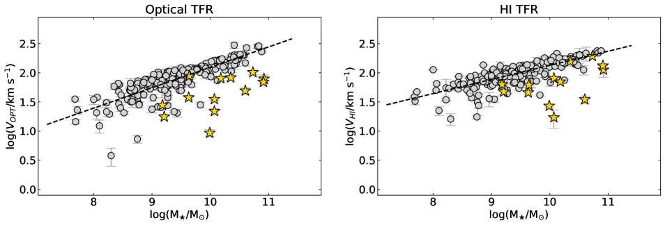
Figure A2: Optical (left) and Hi (right) stellar mass TFRs and linear fits for the kinematic, pruned SAMI-Hi sample, reproduced from the bottom panels of Fig. 6 (gray circles). Yellow stars indicate additional galaxies with incorrect inclination estimates that were discarded after visual inspection (see Fig. A3), consistently with our $i<40$^∘ selection cut.

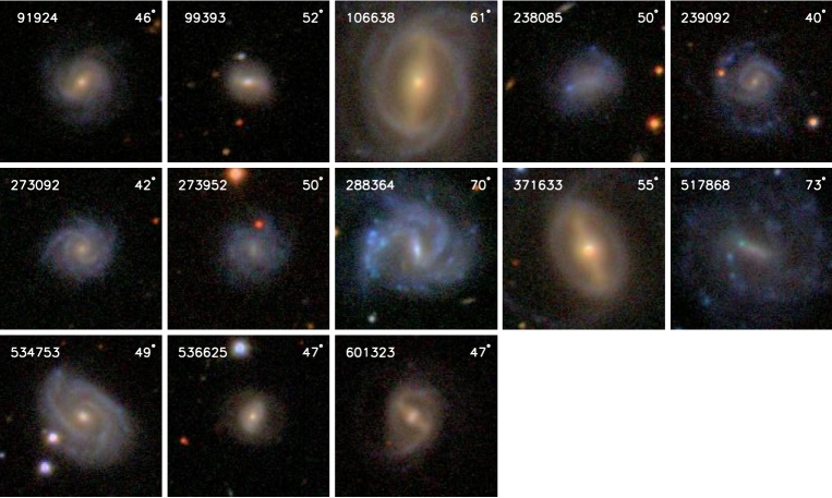
Figure A3: SDSS postage stamp images (1 arcmin square) of the galaxies marked as yellow stars in Fig. A2, with SAMI identifier and inclination noted on the top left and right corners, respectively.

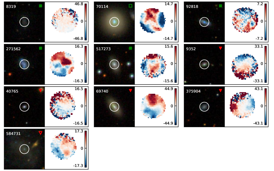
Figure A4: SDSS postage stamp images (1 arcmin square) and SAMI $\rm H\alpha$ velocity fields of kinematically disturbed systems marked with green and red symbols in Fig. 5a. On the SDSS images, SAMI identifiers and symbols used in Fig. 5a are noted on the top-left and top-right corners, respectively; white circles show the $\sim$15 arcsec field-of-view of SAMI. Color bars next to the maps are labelled by $\rm H\alpha$ line-of-sight velocity in km s^-1.

References

- Aaronson et al. (1979) Aaronson M., Huchra J., Mould J., 1979, ApJ, 229, 1
- Aquino-Ortíz et al. (2018) Aquino-Ortíz E., et al., 2018, MNRAS, 479, 2133
- Barat et al. (2019) Barat D., et al., 2019, MNRAS, 487, 2924
- Barat et al. (2020) Barat D., D’Eugenio F., Colless M., Sweet S. M., Groves B., Cortese L., 2020, MNRAS, 498, 5885
- Begum et al. (2008) Begum A., Chengalur J. N., Karachentsev I. D., Sharina M. E., 2008, MNRAS, 386, 138
- Bloom et al. (2017) Bloom J. V., et al., 2017, MNRAS, 472, 1809
- Blyth et al. (2016) Blyth S., et al., 2016, in MeerKAT Science: On the Pathway to the SKA. p. 4
- Booth et al. (2009) Booth R. S., de Blok W. J. G., Jonas J. L., Fanaroff B., 2009, preprint, (arXiv:0910.2935)
- Bottinelli et al. (1983) Bottinelli L., Gouguenheim L., Paturel G., de Vaucouleurs G., 1983, A&A, 118, 4
- Bradford et al. (2016) Bradford J. D., Geha M. C., van den Bosch F. C., 2016, ApJ, 832, 11
- Brook et al. (2016) Brook C. B., Santos-Santos I., Stinson G., 2016, MNRAS, 459, 638
- Bryant et al. (2015) Bryant J. J., et al., 2015, MNRAS, 447, 2857
- Bundy et al. (2015) Bundy K., et al., 2015, ApJ, 798, 7
- Carilli & Rawlings (2004) Carilli C. L., Rawlings S., 2004, New Astron. Rev., 48, 979
- Catinella & Cortese (2015) Catinella B., Cortese L., 2015, MNRAS, 446, 3526
- Catinella et al. (2006) Catinella B., Giovanelli R., Haynes M. P., 2006, ApJ, 640, 751
- Catinella et al. (2007) Catinella B., Haynes M. P., Giovanelli R., 2007, AJ, 134, 334
- Catinella et al. (2010) Catinella B., et al., 2010, MNRAS, 403, 683
- Catinella et al. (2012a) Catinella B., et al., 2012a, MNRAS, 420, 1959
- Catinella et al. (2012b) Catinella B., et al., 2012b, A&A, 544, A65
- Catinella et al. (2018) Catinella B., et al., 2018, MNRAS, 476, 875
- Cecil et al. (2016) Cecil G., et al., 2016, MNRAS, 456, 1299
- Chabrier (2003) Chabrier G., 2003, PASP, 115, 763
- Cortese et al. (2014) Cortese L., et al., 2014, ApJL, 795, L37
- Cortese et al. (2016) Cortese L., et al., 2016, MNRAS, 459, 3574
- Courteau (1997) Courteau S., 1997, AJ, 114, 2402
- Courteau et al. (2007) Courteau S., Dutton A. A., van den Bosch F. C., MacArthur L. A., Dekel A., McIntosh D. H., Dale D. A., 2007, ApJ, 671, 203
- Cresci et al. (2009) Cresci G., et al., 2009, ApJ, 697, 115
- Croom et al. (2012) Croom S. M., et al., 2012, MNRAS, 421, 872
- Croom et al. (2021) Croom S. M., et al., 2021, MNRAS,
- Davies et al. (2016) Davies L. J. M., et al., 2016, MNRAS, 461, 458
- Davis et al. (2011) Davis T. A., et al., 2011, MNRAS, 414, 968
- Driver et al. (2011) Driver S. P., et al., 2011, MNRAS, 413, 971
- Fall (1983) Fall S. M., 1983, in Athanassoula E., ed., Vol. 100, Internal Kinematics and Dynamics of Galaxies. pp 391–398
- Fernández Lorenzo et al. (2009) Fernández Lorenzo M., Cepa J., Bongiovanni A., Castañeda H., Pérez García A. M., Lara-López M. A., Pović M., Sánchez-Portal M., 2009, A&A, 496, 389
- Freeman (1970) Freeman K. C., 1970, ApJ, 160, 811
- Geha et al. (2006) Geha M., Blanton M. R., Masjedi M., West A. A., 2006, ApJ, 653, 240
- Giovanelli et al. (1997a) Giovanelli R., Haynes M. P., Herter T., Vogt N. P., Wegner G., Salzer J. J., da Costa L. N., Freudling W., 1997a, AJ, 113, 22
- Giovanelli et al. (1997b) Giovanelli R., Haynes M. P., Herter T., Vogt N. P., da Costa L. N., Freudling W., Salzer J. J., Wegner G., 1997b, AJ, 113, 53
- Giovanelli et al. (2005) Giovanelli R., et al., 2005, AJ, 130, 2598
- Glowacki et al. (2020) Glowacki M., Elson E., Davé R., 2020, MNRAS, 498, 3687
- Governato et al. (2007) Governato F., Willman B., Mayer L., Brooks A., Stinson G., Valenzuela O., Wadsley J., Quinn T., 2007, MNRAS, 374, 1479
- Gurovich et al. (2004) Gurovich S., McGaugh S. S., Freeman K. C., Jerjen H., Staveley-Smith L., De Blok W. J. G., 2004, PASA, 21, 412
- Guthrie (1992) Guthrie B. N. G., 1992, A&AS, 93, 255
- Hardwick et al. (2022) Hardwick J. A., Cortese L., Obreschkow D., Catinella B., Cook R. H. W., 2022, MNRAS, 509, 3751
- Haynes et al. (2018) Haynes M. P., et al., 2018, ApJ, 861, 49
- Ho et al. (2016) Ho I. T., et al., 2016, Ap&SS, 361, 280
- Holwerda et al. (2012) Holwerda B. W., Blyth S.-L., Baker A. J., 2012, in Tuffs R. J., Popescu C. C., eds, IAU Symposium Vol. 284, IAU Symposium. pp 496–499 (arXiv:1109.5605), doi:10.1017/S1743921312009702
- Hotan et al. (2021) Hotan A. W., et al., 2021, PASA, 38, e009
- Janowiecki et al. (2020) Janowiecki S., Catinella B., Cortese L., Saintonge A., Wang J., 2020, MNRAS, 493, 1982
- Jarvis et al. (2016) Jarvis M., et al., 2016, in MeerKAT Science: On the Pathway to the SKA. p. 6 (arXiv:1709.01901)
- Johnston et al. (2008) Johnston S., et al., 2008, Experimental Astronomy, 22, 151
- Jonas & MeerKAT Team (2016) Jonas J., MeerKAT Team 2016, in MeerKAT Science: On the Pathway to the SKA. p. 1
- Kannappan et al. (2002) Kannappan S. J., Fabricant D. G., Franx M., 2002, AJ, 123, 2358
- Kassin et al. (2007) Kassin S. A., et al., 2007, ApJL, 660, L35
- Kelvin et al. (2012) Kelvin L. S., et al., 2012, MNRAS, 421, 1007
- Koribalski et al. (2020) Koribalski B. S., et al., 2020, Ap&SS, 365, 118
- Korsaga et al. (2019) Korsaga M., Epinat B., Amram P., Carignan C., Adamczyk P., Sorgho A., 2019, MNRAS, 490, 2977
- Lelli et al. (2016a) Lelli F., McGaugh S. S., Schombert J. M., 2016a, AJ, 152, 157
- Lelli et al. (2016b) Lelli F., McGaugh S. S., Schombert J. M., 2016b, ApJL, 816, L14
- Lelli et al. (2019) Lelli F., McGaugh S. S., Schombert J. M., Desmond H., Katz H., 2019, MNRAS, 484, 3267
- Leung et al. (2018) Leung G. Y. C., et al., 2018, MNRAS, 477, 254
- Maddox et al. (2021) Maddox N., et al., 2021, A&A, 646, A35
- Mancera Piña et al. (2019) Mancera Piña P. E., et al., 2019, ApJL, 883, L33
- Mancera Piña et al. (2020) Mancera Piña P. E., et al., 2020, MNRAS, 495, 3636
- Marinacci et al. (2014) Marinacci F., Pakmor R., Springel V., 2014, MNRAS, 437, 1750
- Martinsson et al. (2013) Martinsson T. P. K., Verheijen M. A. W., Westfall K. B., Bershady M. A., Andersen D. R., Swaters R. A., 2013, A&A, 557, A131
- Masters et al. (2019) Masters K. L., et al., 2019, MNRAS, 488, 3396
- McGaugh (2005) McGaugh S. S., 2005, ApJ, 632, 859
- McGaugh et al. (2000) McGaugh S. S., Schombert J. M., Bothun G. D., de Blok W. J. G., 2000, ApJL, 533, L99
- Meyer (2009) Meyer M., 2009, in Panoramic Radio Astronomy: Wide-field 1-2 GHz Research on Galaxy Evolution. p. 15 (arXiv:0912.2167)
- Mo et al. (1998) Mo H. J., Mao S., White S. D. M., 1998, MNRAS, 295, 319
- Navarro & Steinmetz (2000) Navarro J. F., Steinmetz M., 2000, ApJ, 538, 477
- Noordermeer et al. (2007) Noordermeer E., van der Hulst J. M., Sancisi R., Swaters R. S., van Albada T. S., 2007, MNRAS, 376, 1513
- Papastergis et al. (2016) Papastergis E., Adams E. A. K., van der Hulst J. M., 2016, A&A, 593, A39
- Pizagno et al. (2007) Pizagno J., et al., 2007, AJ, 134, 945
- Ponomareva et al. (2018) Ponomareva A. A., Verheijen M. A. W., Papastergis E., Bosma A., Peletier R. F., 2018, MNRAS, 474, 4366
- Ponomareva et al. (2021) Ponomareva A. A., et al., 2021, MNRAS, 508, 1195
- Reyes et al. (2011) Reyes R., Mandelbaum R., Gunn J. E., Pizagno J., Lackner C. N., 2011, MNRAS, 417, 2347
- Romanowsky & Fall (2012) Romanowsky A. J., Fall S. M., 2012, ApJS, 203, 17
- Saintonge (2007) Saintonge A., 2007, AJ, 133, 2087
- Saintonge & Catinella (2022) Saintonge A., Catinella B., 2022, ARA&A, 60, 319
- Simons et al. (2015) Simons R. C., Kassin S. A., Weiner B. J., Heckman T. M., Lee J. C., Lotz J. M., Peth M., Tchernyshyov K., 2015, MNRAS, 452, 986
- Springob et al. (2005) Springob C. M., Haynes M. P., Giovanelli R., Kent B. R., 2005, ApJS, 160, 149
- Stark et al. (2009) Stark D. V., McGaugh S. S., Swaters R. A., 2009, AJ, 138, 392
- Stark et al. (2021) Stark D. V., et al., 2021, MNRAS, 503, 1345
- Stevens et al. (2019) Stevens A. R. H., Diemer B., Lagos C. d. P., Nelson D., Obreschkow D., Wang J., Marinacci F., 2019, MNRAS, 490, 96
- Taranu et al. (2017) Taranu D. S., et al., 2017, ApJ, 850, 70
- Teerikorpi (1984) Teerikorpi P., 1984, A&A, 141, 407
- Teerikorpi (1997) Teerikorpi P., 1997, ARA&A, 35, 101
- Tiley et al. (2016) Tiley A. L., Bureau M., Saintonge A., Topal S., Davis T. A., Torii K., 2016, MNRAS, 461, 3494
- Tiley et al. (2019) Tiley A. L., et al., 2019, MNRAS, 482, 2166
- Tiley et al. (2021) Tiley A. L., et al., 2021, MNRAS, 506, 323
- Topal et al. (2018) Topal S., Bureau M., Tiley A. L., Davis T. A., Torii K., 2018, MNRAS, 479, 3319
- Tully & Fisher (1977) Tully R. B., Fisher J. R., 1977, A&A, 54, 661
- Übler et al. (2017) Übler H., et al., 2017, ApJ, 842, 121
- Varidel et al. (2020) Varidel M. R., et al., 2020, MNRAS, 495, 2265
- Verheijen (2001) Verheijen M. A. W., 2001, ApJ, 563, 694
- Verheijen et al. (2008) Verheijen M. A. W., Oosterloo T. A., van Cappellen W. A., Bakker L., Ivashina M. V., van der Hulst J. M., 2008, in Minchin R., Momjian E., eds, American Institute of Physics Conference Series Vol. 1035, The Evolution of Galaxies Through the Neutral Hydrogen Window. pp 265–271 (arXiv:0806.0234), doi:10.1063/1.2973599
- Wang et al. (2016) Wang J., Koribalski B. S., Serra P., van der Hulst T., Roychowdhury S., Kamphuis P., Chengalur J. N., 2016, MNRAS, 460, 2143
- Watts et al. (2022) Watts A. B., et al., 2022, MNRAS
- Weijmans et al. (2014) Weijmans A.-M., et al., 2014, MNRAS, 444, 3340
- Westmeier et al. (2022) Westmeier T., et al., 2022, PASA, 39, e058
- York et al. (2000) York D. G., et al., 2000, AJ, 120, 1579
- Zaritsky et al. (2014) Zaritsky D., et al., 2014, AJ, 147, 134
- da Cunha et al. (2008) da Cunha E., Charlot S., Elbaz D., 2008, MNRAS, 388, 1595