Physics-based Indirect Illumination for Inverse Rendering

Abstract

We present a physics-based inverse rendering method that learns the illumination, geometry, and materials of a scene from posed multi-view RGB images. To model the illumination of a scene, existing inverse rendering works either completely ignore the indirect illumination or model it by coarse approximations, leading to sub-optimal illumination, geometry, and material prediction of the scene. In this work, we propose a physics-based illumination model that first locates surface points through an efficient refined sphere tracing algorithm, then explicitly traces the incoming indirect lights at each surface point based on reflection. Then, we estimate each identified indirect light through an efficient neural network. Moreover, we utilize the Leibniz’s integral rule to resolve non-differentiability in the proposed illumination model caused by boundary lights inspired by differentiable irradiance in computer graphics. As a result, the proposed differentiable illumination model can be learned end-to-end together with geometry and materials estimation. As a side product, our physics-based inverse rendering model also facilitates flexible and realistic material editing as well as relighting. Extensive experiments on synthetic and real-world datasets demonstrate that the proposed method performs favorably against existing inverse rendering methods on novel view synthesis and inverse rendering. The source code and trained models can be found at the project page: https://denghilbert.github.io/pii.

1 Introduction

Inverse rendering aims to recover the illumination, geometry, and material simultaneously of a scene from multiview images. Illumination plays an important role in inverse rendering by providing crucial lighting information for material and geometry estimation. However, it is challenging to accurately estimate illumination in a scene due to complex scene geometry and various materials that lead to light occlusion and reflection. Early inverse rendering works [21, 12] adopt a simple illumination model [1] and can only be applied to scenes with simple geometry (e.g., scenes that only include a single object). Some recent approaches [24, 46, 49, 41, 17, 45] simulate natural illumination and enable material editing and relighting by utilizing the rendering equation [14]. However, most of these methods [46, 17, 45] only model direct illumination and ignore indirect environment lights caused by occlusion and reflection, leading to poor performance on self-occluded scenes. Even when indirect lights are implicitly modeled as in [49, 41, 24, 33], they are approximated with multi-layer perceptrons (MLPs), ignoring natural occlusion and reflection in the scene. One example is shown in the top row of Fig. 1b and Fig. 1c where the baseline model [49] fails to capture reflection and produces noticeable artifacts in both inverse rendering and material editing.

We propose a physics-based inverse rendering framework to accurately model indirect illumination and simultaneously estimate the material and geometry of a scene. For indirect illumination modeling, our method first locates all surface points by a novel and efficient refined sphere tracing algorithm. It then explicitly traces the incoming indirect lights at each surface point based on reflection. Finally, we propose to estimate each traced indirect light by aggregating environment lights using weights predicted by an MLP. However, such a physics-based indirect illumination model is not inherently differentiable due to boundary lights [19, 44] – the environment lights that fall rightly onto the brim of an object (purple ray in Fig. 1a). Inspired by differentiable irradiance in graphics [4, 44], we derive the gradients of boundary lights theoretically by using the Leibniz’s integral rule. As a result, the proposed illumination module (green block of Fig. 2) can be learned end-to-end together with an SDF prediction MLP (blue block of Fig. 2) and a material estimation autoencoder (yellow block of Fig. 2). During inference, our method can be readily applied to novel view synthesis, material editing, and relighting, showing favorable performance compared to existing methods on both synthetic and real-world datasets.

The main contributions of this work are:

• We present a method for high-fidelity geometry, materials, and illumination estimation.

• We develop an efficient sphere tracing algorithm for fast surface point locating and an end-to-end differentiable method that models indirect illumination by explicitly tracing and estimating the incoming indirect lights at each surface point.

• The proposed method performs favorably against existing methods on inverse rendering, novel-view synthesis, and material editing.

2 Related Work

Implicit Neural Networks. Implicit neural networks encode the geometry of a scene by predicting either occupancy or a signed distance of each surface point. Early implicit neural networks [27, 30] are learned with ground truth occupancy or signed distances, while more recent models [28, 42] are trained with multi-view images by utilizing volume rendering [26]. However, by entangling geometry with appearance and illumination in neural networks, these methods do not perform well on tasks such as material editing and free-viewpoint relighting. In this paper, we disentangle the geometry, material, and illumination by learning an inverse rendering framework. The geometry is captured by an implicit neural network that predicts the signed distance value for each surface point.

Intrinsic Decomposition and Inverse Rendering. Intrinsic image decomposition [1] aims to model an image as the product of reflectance and shading. This is a highly ill-posed problem if ground truth annotation is not available. As a result, deep intrinsic decomposition models usually resort to synthetic dataset [2, 8, 9, 16, 29] or time-lapse sequences [20]. To better model image formulation and enable self-supervised decomposition from images, more recent methods further decompose shading into illumination and geometry, i.e., inverse rendering. One line of self-supervised inverse rendering work [35, 40] utilizes the prior of a specific object category (e.g., faces, cars, etc) to constrain illumination prediction. To apply inverse rendering on more general scenes, several methods use multi-view images as supervision [15, 43]. Recently, PhySG [45] and NeRFactor [48] merge implicit geometry with the rendering equation [14] to decompose material properties and illuminations from visual appearance. PhySG [45] resolves inverse rendering by modeling illumination as mixtures of spherical Gaussians [38], combined with an implicit function for geometry estimation. However, PhySG does not explicitly model indirect illumination, which plays an important role in capturing reflection in a scene. To resolve this issue, several approaches [49, 41, 33, 24, 48] approximate the indirect illumination and visibility in the scene through MLPs. Other methods use more physical-based modeling [39, 23]. Nonetheless, without explicitly tracing and estimating indirect environment lights, these methods do not accurately capture the reflections in the scene and produce artifacts in both inverse rendering and material editing. In contrast, we propose a self-supervised inverse rendering method that explicitly traces and estimates the indirect lights at each surface point, showing promising results in both inverse rendering and material editing.

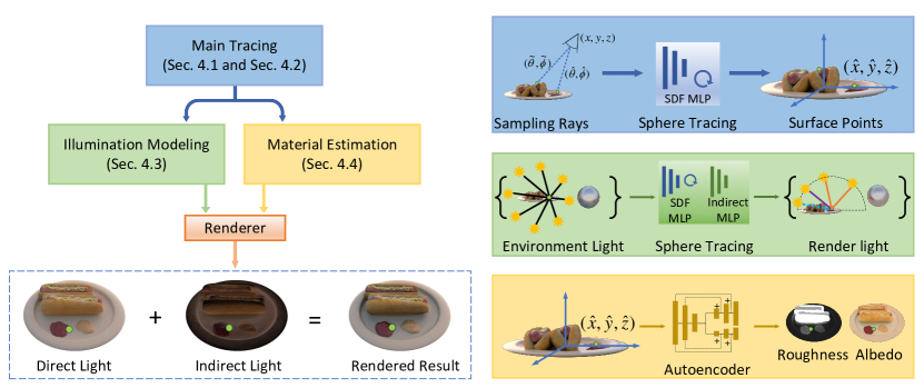
Figure 2: Forward Rendering of Our Framework. Given the camera parameters of a scene view, we sample a set of rays and trace the surface points hit by the rays by the refined sphere tracing module introduced in Sec. 4.2. We estimate each traced point’s illumination through the illumination module in Sec. 4.3 and materials by the material estimation module in Sec. 4.4. Finally, we feed the estimated materials and illuminations to a differentiable renderer and render a target view image.

3 Preliminaries

3.1 Rendering Equation

Before describing our method, we briefly review the Bidirectional Reflectance Distribution Function (BRDF) and the rendering equation that computes outgoing radiance at each surface point in the scene.

Given a surface point $\boldsymbol{x}$ and the outgoing light direction $\boldsymbol{\omega}_{o}$, the rendering equation [14] computes the outgoing light $L_{o}(\boldsymbol{\omega}_{o};\boldsymbol{x})$ as the integral over all environment lights $L_{i}(\boldsymbol{\omega}_{i})$ from the upper hemisphere $\Omega$:

$$L_{o}(\boldsymbol{\omega}_{o};\boldsymbol{x})=\int_{\Omega}L_{i}(\boldsymbol{\omega}_{i})f_{r}(\boldsymbol{\omega}_{o},\boldsymbol{\omega}_{i};\boldsymbol{x})(\boldsymbol{\omega}_{i}\cdot\boldsymbol{n}){\rm d}\boldsymbol{\omega}_{i},$$ (1)

where $f_{r}(\boldsymbol{\omega}_{o},\boldsymbol{\omega}_{i};\boldsymbol{x})$ is the simplified Disney BRDF [3] that models the reflectance property of the surface point $\boldsymbol{x}$ and $\boldsymbol{n}$ is the normal at this point. The specularity term in $f_{r}(\boldsymbol{\omega}_{o},\boldsymbol{\omega}_{i};\boldsymbol{x})$ is modeled with the microfacet model [6, 37]. More details can be found in the supplementary.

3.2 Spherical Gaussians Function

We model the environment light $L_{i}(\boldsymbol{\omega}_{i})$, BRDF $f_{r}(\boldsymbol{\omega}_{o},\boldsymbol{\omega}_{i};\boldsymbol{x})$, and multiplication term $\boldsymbol{\omega}_{i}\cdot\boldsymbol{n}$ in Eq. 1 by the Spherical Gaussian (SG) Distribution [38]. A Spherical Gaussian is defined as:

$$G(\boldsymbol{\omega}_{i};\boldsymbol{\xi},\lambda,\boldsymbol{\mu})=\boldsymbol{\mu}e^{\lambda(\boldsymbol{\omega}_{i}\cdot\boldsymbol{\xi}-1)},$$ (2)

where $\boldsymbol{\omega}_{i}\in\mathbb{S}^{2}$ is the input of the SG function, $\boldsymbol{\xi}\in\mathbb{S}^{2}$ is the lobe axis, $\lambda\in\mathbb{R}_{+}$ is the lobe sharpness, and $\boldsymbol{\mu}\in\mathbb{R}^{3}$ is the lobe amplitude.

When modeling the environment lights using the SG function, we assume the lights are uniformly cast from 128 infinitely faraway directions. We analyze the number of environment lights in Sec. 5.2. For computational efficiency, we further represent the BRDF $f_{r}$, and the multiplication term $\boldsymbol{\omega}_{i}\cdot\boldsymbol{n}$ in Eq. 1 with SG as in [45]. More details can be found in the supplementary material.

4 Proposed Method

Given multiple images of a scene, we learn a self-supervised inverse rendering framework that estimates the geometry, materials, and illumination of the scene. During inference, our model is readily available for novel view synthesis, relighting, and material editing. We show the overview of our pipeline in Fig. 2 and introduce details for geometry estimation (Sec. 4.1), surface point localization (Sec. 4.2), illumination modeling (Sec. 4.3) and materials prediction (Sec. 4.4) below.

4.1 Geometry Estimation

We encode the geometry of a given scene by learning an MLP $F_{SDF}$ that takes a query point $\boldsymbol{p}=(x,y,z)$ as input and predicts its SDF value (i.e., the closest distance between $\boldsymbol{p}$ and the object surface). We first initialize this geometry MLP using multi-view images as in [46, 49, 41]. We then fine-tune the MLP with the illumination and material estimation modules in the following sections.

4.2 Sphere Tracing with Refinement

We discuss locating all surface points using the learned geometry MLP discussed in Sec. 4.1 and a novel refined sphere tracing module.

Given camera parameters, classical sphere tracing algorithms [10, 22] trace all surface points by marching along sampled rays iteratively until reaching a point with an SDF value smaller than a given threshold $\tau$. We demonstrate this tracing process in Fig. 3(a) and show the traced surface point $\boldsymbol{p}_{1}$ as well as the “true” surface point $\boldsymbol{p}_{2}$ in Fig. 3(b). As shown in Fig. 3, a larger threshold $\tau$ leads to a more inaccurate surface point location (i.e., $\boldsymbol{p}_{1}$ is farther from the object surface), while a smaller threshold requires more tracing iterations. To efficiently and accurately locate a surface point, we propose a refinement process that directly steps from $\boldsymbol{p}_{1}$ to $\boldsymbol{p}_{2}$. Our main observation is that as $\boldsymbol{p}_{1}$ moves closer to $\boldsymbol{p}_{2}$, the surface curve $\boldsymbol{s}\boldsymbol{p}_{2}$ approximates to a straight line. Thus we can find the length of $\overline{\boldsymbol{p}_{1}\boldsymbol{p}_{2}}$ by:

$$\overline{\boldsymbol{p}_{1}\boldsymbol{p}_{2}}=\frac{-F_{SDF}(\boldsymbol{p}_{1})}{\boldsymbol{v}\cdot\boldsymbol{n}},\ \ \boldsymbol{n}=\frac{\nabla_{\boldsymbol{p}}F_{SDF}(\boldsymbol{p})}{||\nabla_{\boldsymbol{p}}F_{SDF}(\boldsymbol{p})||_{2}},$$ (3)

where $\boldsymbol{v}$ is the normalized view direction, and the normal $\boldsymbol{n}$ at point $\boldsymbol{s}$ can be derived from the learned geometry MLP $F_{SDF}$ discussed in Sec. 4.1.

Compared to classic sphere tracing methods [10, 22], the proposed refinement step uses a relatively large threshold and requires fewer tracing iterations and less time. We demonstrate its effectiveness in Sec. 5.2.

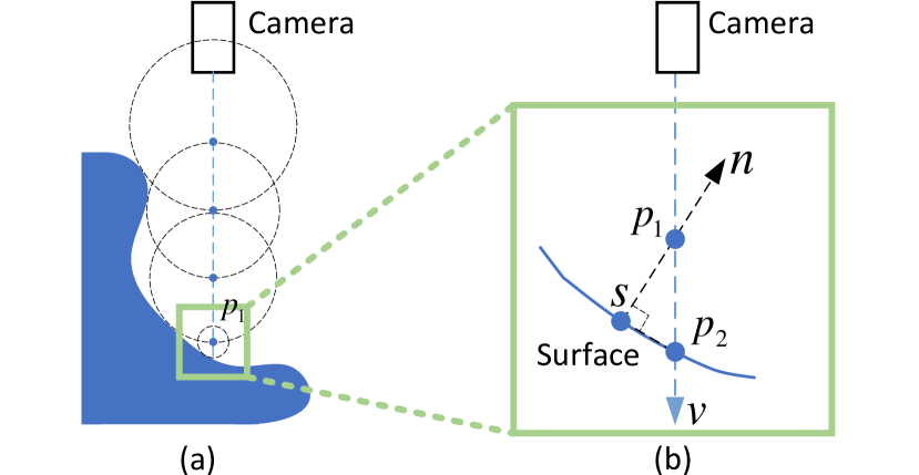
Figure 3: Sphere Tracing with Refinement. The classic sphere tracing algorithm stops at $\boldsymbol{p}_{1}$ when the SDF value of this point is smaller than the threshold. We propose a refinement process that directly marches from $\boldsymbol{p}_{1}$ to point $\boldsymbol{p}_{2}$ that is closer to the surface.

4.3 Illumination Modeling

Illumination plays a critical role in recovering the geometry and materials of a scene from a set of RGB images. However, it is challenging to accurately model the environment lights due to indirect reflection. Existing approaches either ignore the indirect lights [46, 17, 45] or implicitly approximate them [49, 41, 24] via neural networks. Instead, we explicitly trace and estimate the incoming indirect lights at each surface point based on occlusion and reflection. In the following, we only focus on indirect lights and omit direct lights that are straightforward to model by Eq. 1.

4.3.1 Indirect Lights Identification

For each environment light, we first classify it as a direct or indirect light by a simplified ray tracing process that explicitly models reflection.

Given a surface point $\boldsymbol{x}$, we reversely trace each environment light starting from $\boldsymbol{x}$ to the light sources. Rays not obstructed by an object are classified as direct lights (orange rays in Fig. 1(a)), and obstructed rays are denoted as indirect lights (blue rays in Fig. 1(a)). We note that here we do not trace the full path of indirect light as classic ray tracing methods [18]. As long as a ray starting from the surface point hits an object while reaching the light sources, we classify the environment light as an indirect light and model it using the method discussed in Sec. 4.3.2. Although this efficient tracing process is simpler compared to methods that trace the complete path, we demonstrate its effectiveness with extensive experiments in Sec. 5.

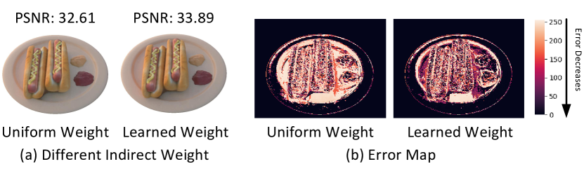
Figure 4: Environment Weight. We visualize rendering results and their error maps with uniform and learned weights.

4.3.2 Indirect Lights Estimation

Given each identified indirect light at the surface point $\boldsymbol{x}$ coming from a reflected point $\boldsymbol{x}^{\prime}$ of Fig. 1(a), we learn an MLP, $F_{ind}$, that explicitly formulates the indirect light by aggregating environment lights. Specifically, for a target indirect light $L_{r}$, the MLP takes the coordinates and normal of the reflected point $\boldsymbol{x}^{\prime}$ as inputs and predicts how much each environment light $L^{i}$ contributes to $L_{r}$ represented as a scalar weight $w_{r}^{i}\in\mathbb{R}$. Thus, the lobe sharpness $\lambda_{r}$ and amplitude $\boldsymbol{\mu}_{r}$ of $L_{r}$ can be computed as:

$$\lambda_{r}=\sum_{i=1}^{K}w_{r}^{i}\cdot\lambda^{i},\boldsymbol{\mu}_{r}=\sum_{i=1}^{K}w_{r}^{i}\cdot\boldsymbol{\mu}^{i},$$ (4)

$$\boldsymbol{w_{r}}=F_{ind}(\gamma(\boldsymbol{x}^{\prime}),\gamma(\boldsymbol{n}^{\prime})),$$ (5)

where $\boldsymbol{n}^{\prime}$ is the normal at $\boldsymbol{x}^{\prime}$ with positional embedding $\gamma$ [34], and $K$ is the total environment light number (e.g., 128 in this work). We carry out further ablation study in Sec. 5.2 to verify the effectiveness of this integral weight design on modeling indirect illumination.

Overall, the proposed indirect light model has two advantages compared to existing inverse rendering methods [49, 41, 33, 24]. First, reflection in the scene is explicitly modeled through the explicit tracing and classification process discussed in Sec. 4.3.1. Second, instead of simply approximating all indirect lights at the surface point (i.e. $x$ in Fig. 1) by an MLP [49], we trace to find reflected points (i.e. $x^{\prime}$ in Fig. 1) and estimate each identified indirect light through learnable integral weights (i.e. $w_{r}$ in  Eq. 5), leading to an illumination model with a higher capacity to handle reflection. Fig. 4, Fig. 6, and Fig. 8 empirically demonstrate the superiority of our indirect light model.

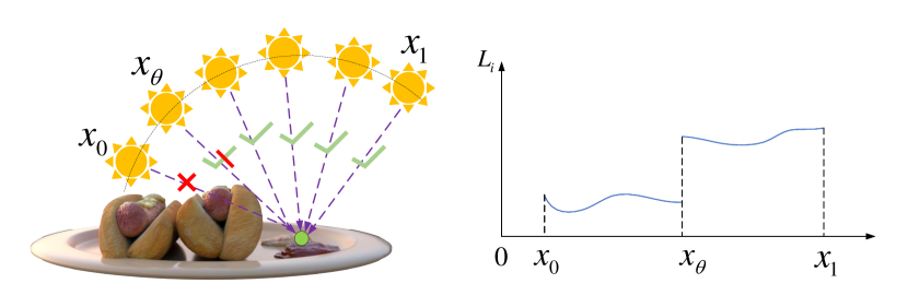
Figure 5: Demonstration of Non-differentiability at Boundary Lights. The boundary light $x_{\theta}$ changes abruptly from “obstructed” to “visible” at the boundary of the object, introducing a point of discontinuity and making Eq. 1 non-differentiable. This non-differentiability is also demonstrated by the figure on the right showing light intensity change w.r.t. the incoming light angle $x_{i}$.

4.3.3 Boundary Lights Differentiation

Ideally, the identified direct lights in Sec. 4.3.1 and estimated indirect lights in Sec. 4.3.2 can be aggregated by  Eq. 1 and learned through backpropagation. However, the boundary lights that fall right onto the brim of an object make Eq. 1 non-differentiable since they change abruptly at the object boundary from “obstructed” to “visible”, as shown in Fig. 5. Naively ignoring the boundary lights does not consider errors from boundary lights and leads to inaccurate illumination estimation (see the last row of Tab. 1(d)). Inspired by recent advances of differential irradiance in computer graphics [4, 44], we use the Leibniz’s integral rule and compute the gradient of the outgoing radiance w.r.t. all learnable parameters $\boldsymbol{\theta}$ as:

$$\frac{\partial L_{o}(\boldsymbol{\omega}_{o};\boldsymbol{x})}{\partial\boldsymbol{\theta}}=\int_{\Omega^{\prime}}\frac{\partial L_{i}(\boldsymbol{\omega}_{i})f_{r}(\boldsymbol{\omega}_{o},\boldsymbol{\omega}_{i};\boldsymbol{x})}{\partial\boldsymbol{\theta}}(\boldsymbol{\omega}_{i}\cdot\boldsymbol{n}){\rm d}\boldsymbol{\omega}_{i}$$ (6)

$$+\int_{\partial\Omega}(\frac{\partial\boldsymbol{\omega}_{i}}{\partial\boldsymbol{\theta}}\cdot\boldsymbol{n}(\boldsymbol{\omega}_{i}))\Delta L_{i}(\boldsymbol{\omega}_{i})f_{r}(\boldsymbol{\omega}_{o},\boldsymbol{\omega}_{i};\boldsymbol{x})(\boldsymbol{\omega}_{i}\cdot\boldsymbol{n}){\rm d}\boldsymbol{\omega}_{i},$$

where $\partial\Omega$ represents the edge ($x_{\theta}$ in Fig. 5) at which the light changes from “obstructed” to “visible”, $\Delta L_{i}(\boldsymbol{\omega}_{i})=L_{i}(\boldsymbol{\omega}_{i}+\boldsymbol{\epsilon})-L_{i}(\boldsymbol{\omega}_{i}-\boldsymbol{\epsilon})$ is the light difference of directions on $\partial\Omega$, and $\Omega^{\prime}=\Omega-\partial\Omega$. The supplementary material presents the detailed mathematical deduction of Eq. 6.

To identify the boundary lights, we simply classify environment lights that are “almost” perpendicular (e.g., a 2-degree deviation) to the surface normal.

4.4 Material Estimation

Similar to [49], we predict its roughness and albedo using a material autoencoder [11] at each point, as shown in the yellow block of Fig. 2. Specifically, we first map the positional encoding [34] of the surface point coordinates into a latent vector through the material encoder. Then we decode the latent vector into roughness and albedo using two separate decoders. Given the estimated materials and illumination discussed in Sec. 4.3, we then render the scene from any given view direction with the rendering equation [14].

4.5 Training

We pre-train the geometry MLP $F_{SDF}$ discussed in Sec. 4.1 following the MII [49]. This provides decent geometry information for the material and illumination module training. Next, we jointly train the geometry MLP, the material, and the illumination module by minimizing the L1 reconstruction loss $\ell_{rec}$. We further encourage the material autoencoder to produce smooth roughness and albedo by applying a latent sparsity constraint with KL divergence $\ell_{KL}$ [7], and a smoothness loss $\ell_{smooth}$ [49]. The overall objective is:

$$\ell=\lambda_{rec}\ell_{rec}+\lambda_{KL}\ell_{KL}+\lambda_{smooth}\ell_{smooth},$$ (7)

$$\ell_{KL}=\sum_{i=1}^{N}KL(\rho||z_{i}),$$ (8)

$$\ell_{smooth}=||D(\boldsymbol{\boldsymbol{z}})-D(\boldsymbol{\boldsymbol{z}}+\boldsymbol{\epsilon})||,$$ (9)

where $N$ is the dimension of latent vector $\boldsymbol{z}$, and $D$ represents the decoders in the material autoencoder. We set $\rho$ to be 0.05 and $\boldsymbol{\epsilon}$ to be 0.02. The weights are set to be $\lambda_{rec}=1.0$, $\lambda_{KL}=0.01$, $\lambda_{smooth}=0.1$.

To summarize, given multi-view images of a scene, our framework models its: (1) illumination via a set of learnable environment lights $L^{i}$ represented as SGs $\{\boldsymbol{\xi}_{i},\lambda_{i},\boldsymbol{\mu}_{i}\}^{128}_{i=1}$, (2) geometry via an MLP $F_{SDF}$, (3) material property (i.e., albedo $\boldsymbol{a}$ and roughness $R$ for each surface point) via a material autoencoder.

#Train/Test (HxW)	Synthetic Chair			Synthetic Jugs			Synthetic Air Balloons			Synthetic Hotdog
	200/200 (800x800)			100/200 (800x800)			100/200 (800x800)			100/200 (800x800)
Metrics	$\downarrow$LPIPS	$\uparrow$SSIM	$\uparrow$PSNR	$\downarrow$LPIPS	$\uparrow$SSIM	$\uparrow$PSNR	$\downarrow$LPIPS	$\uparrow$SSIM	$\uparrow$PSNR	$\downarrow$LPIPS	$\uparrow$SSIM	$\uparrow$PSNR
PhySG* [45]	0.0406	0.9497	32.08	0.0515	0.9742	33.59	0.0439	0.9618	31.79	0.0317	0.9564	31.95
MII [49]	0.0147	0.9482	35.42	0.0193	0.9714	37.47	0.0468	0.9498	31.03	0.0216	0.9531	32.69
Ours (Learned)	0.0125	0.9534	36.04	0.0148	0.9788	38.76	0.0364	0.9613	32.72	0.0192	0.9589	33.76
Ours (Uniform)	0.0173	0.9526	33.62	0.0301	0.9728	33.79	0.0487	0.9566	30.13	0.0221	0.9564	32.74

(a) Novel View Synthesis.

#Train/Test (HxW)	Synthetic Chair			Synthetic Jugs			Synthetic Air Balloons			Synthetic Hotdog
	200/200 (800x800)			100/200 (800x800)			100/200 (800x800)			100/200 (800x800)
Metrics	$\downarrow$LPIPS	$\uparrow$SSIM	$\uparrow$PSNR	$\downarrow$LPIPS	$\uparrow$SSIM	$\uparrow$PSNR	$\downarrow$LPIPS	$\uparrow$SSIM	$\uparrow$PSNR	$\downarrow$LPIPS	$\uparrow$SSIM	$\uparrow$PSNR
PhySG* [45]	0.1004	0.9159	24.58	0.2119	0.9415	27.38	0.1395	0.9405	24.51	0.1517	0.9229	19.51
MII [49]	0.1158	0.9063	24.96	0.2302	0.9216	26.719	0.1636	0.9218	22.53	0.0770	0.9401	23.64
Ours	0.0881	0.9083	25.07	0.2138	0.9477	26.80	0.1147	0.9513	26.43	0.0887	0.9415	22.77
Ours (w/o boundary)	0.0997	0.9131	25.01	0.2195	0.9436	26.83	0.1173	0.9494	26.22	0.1008	0.9345	22.72

(b) Albedo Estimation.

scenes	Synthetic Chair		Synthetic Jugs		Synthetic Air Balloons		Synthetic Hotdog
Metrics	$\downarrow$MSE	$\downarrow$ARE	$\downarrow$MSE	$\downarrow$ARE	$\downarrow$MSE	$\downarrow$ARE	$\downarrow$MSE	$\downarrow$ARE
PhySG* [45]	0.0921	1.1771	0.1200	1.2974	0.1832	3.0347	0.2861	24.6206
MII [49]	0.0306	1.1861	0.0617	1.1789	0.0242	0.8936	0.0776	4.7174
Ours	0.0421	1.0829	0.0484	0.9123	0.0132	0.6450	0.0819	4.5096

(c) Roughness Estimation.

Scenes	Chair	Jugs	Air Balloons	Hotdog
Metric	$\downarrow$Light Estimation MSE
PhySG* [45]	0.0557	0.1067	0.0154	0.0493
MII [49]	0.0562	0.1371	0.0186	0.0256
Ours	0.0232	0.0555	0.0120	0.0144
Ours (w/o boundary)	0.0386	0.0699	0.0213	0.0427

(d) Light Estimation.

Table 1: Quantitative Results. We compare our method with PhySG* [45] (slightly modified, see Sec. 5.1) and MII [49] on four tasks: novel view synthesis, albedo, and roughness estimation, as well as environment map estimation. HDR images used in synthetic data are tone mapped with $I_{new}=I_{old}^{1/2.2}$ and clipped to $\left[0,1\right]$.

5 Experimental Results

We evaluate our method on the synthetic scenes in [49]. All the scenes are rendered with natural environment lights and provided with foreground masks. For quantitative evaluation, the dataset provides 200 testing images along with the ground truth albedo and roughness. The images have a resolution of 800$\times$800.

5.1 Comparisons with State-of-the-art Methods

Baseline methods. We compare with two state-of-the-art inverse rendering methods: PhySG [45] and MII [49]. Both methods predict illumination, materials, and geometry from multi-view images. Following MII [49], we replace the global roughness module in PhySG [45] with our spatial-varying material net since the original one cannot estimate spatially-varying surface roughness.

Metrics. We conduct extensive experiments to compare the proposed method and baselines on novel view synthesis, materials estimation, and environment light prediction. Specifically, for novel view synthesis and albedo prediction, we report the PSNR, SSIM, and LPIPS [47] between the ground truth and predictions. For roughness estimation, we adopt the mean square error (MSE) and the absolute relative error [31] as evaluation metrics. While for illumination estimation, we compare the MSE between the ground truth and predicted environment maps as in [5].

Quantitative Results. We report quantitative evaluation on novel view synthesis, materials, and illumination evaluation in Tab. 1. We use ground truth images, albedo, roughness, and environment maps to compute the abovementioned metrics. As shown in Tab. 1(a) and Tab. 1(d), our method consistently outperforms the baseline models on all testing scenes on novel view synthesis and illumination estimation. For material estimation, our method performs favorably against baselines on all testing scenes and most metrics quantitatively, as demonstrated in Tabs. 1(b) and 1(c). The supplementary material will show the other two air balloons and chairs scenes.

Qualitative Results. As shown in Fig. 6, our model predicts plausible roughness and material while PhySG [45] suffers from disentangling illumination and materials where the lights are obstructed (e.g., the occluded jug bottoms and the white balloon in the middle). Furthermore, compared to MII [49], our method estimates more consistent roughness and realistic albedo by explicitly tracing and estimating indirect lights based on occlusion and reflectance.

Indirect Reflection. We show that our model effectively captures the indirect reflection in a scene by changing the Fresnel coefficient [3] in the Fresnel term. To this end, we increase the coefficient to enhance surface reflection, as shown in Fig. 1c and Fig. 8c. Surprisingly, our model can capture the indirect reflection in every scene. We observe the reflected heart-shaped pattern in the balloon scene in Fig. 1c, the shadows of the back of the chair and pillow accurately casting onto the seat, and the precise edge shape of the hotdog projecting on the plate (green boxes in Fig. 8c). In contrast, the same editing applied to the MII [49] generates noisy black points and noticeable artifacts for indirect reflection. This empirically demonstrates that the proposed method successfully mimics the reflectance in the physical world, which is rarely achieved by existing models [49, 41, 24].

Relighting and Editing. Thanks to the rendering equation, our model facilitates flexible editing for both material and illumination during inference. We demonstrate how to edit the learned albedo in Fig. 8a, the environment light in Fig. 8b, and the roughness in Fig. 8d. Our framework can get reasonable rendering results with different base colors or environment illumination. More results and videos are available in the supplementary material.

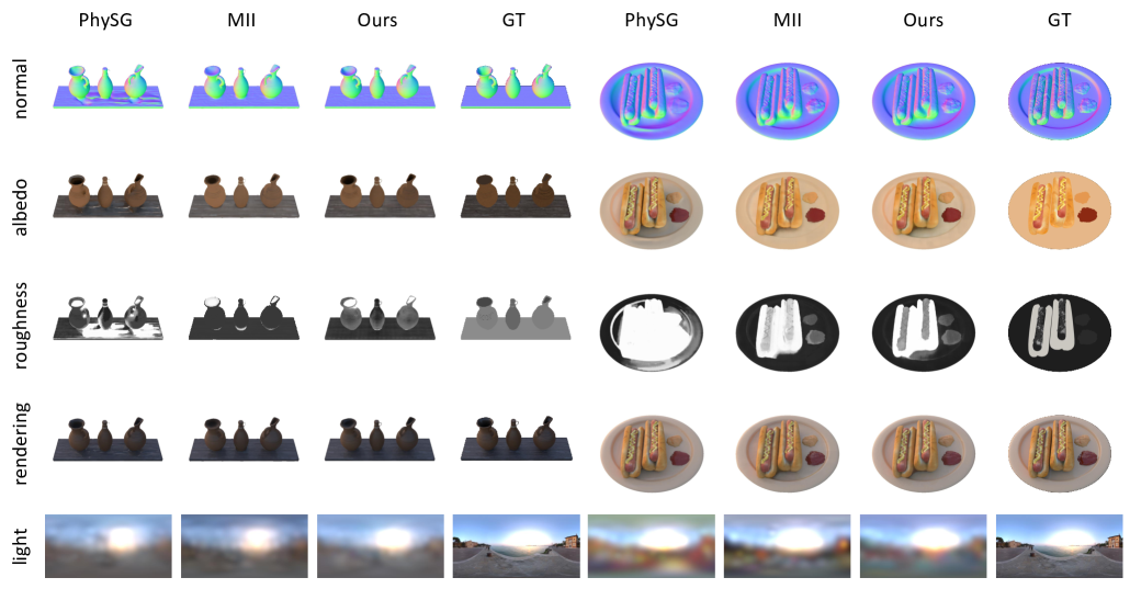
Figure 6: Qualitative Comparisons on Synthetic Dataset. We show qualitative comparisons of PhySG [45], MII [49], and our method on novel view synthesis, albedo, roughness, and environment map estimation. More scenes can be found in the supplementary.

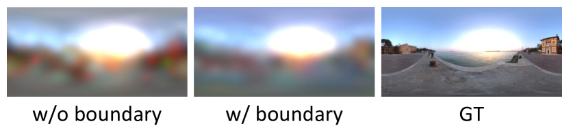
Figure 7: Ablation on Boundary Lights. Without boundary lights, optimized environment maps have noticeable artifacts.

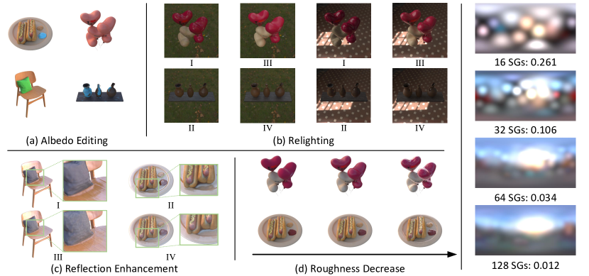
Figure 8: Material Editing and Relighting. Left: (a) Base color editing results by changing the albedo. (b) Relighting results (i@, ii@) by changing the illumination SGs and GT (iii@, iv@) rendered with Blender [5]. (c) Enhancement of reflection and comparison between MII [49] (i@, ii@) and our model (iii@, iv@). (d) The gradual decrease of the surface roughness and the objects’ surface change from matte to smooth. Right: We experiment with different SG numbers for illumination to find a balance between a high-fidelity model and memory efficiency.

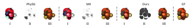
Figure 9: Qualitative Comparisons on DTU [13]. Even for the real-world dataset, our method can still decompose reasonable albedo (i@), roughness(ii@), and realistic rendering result (iii@). In contrast, previous methods [49, 45] struggle to preserve consistent roughness and albedo. Our method generalizes well to challenging real-world dataset, producing reasonable albedo (i@), roughness(ii@), and realistic rendering result (iii@). In contrast, the baselines [49, 45] struggle to predict consistent roughness and albedo.

5.2 Ablation Studies

Sphere Tracing Refinement. By allowing a large threshold to reduce tracing iterations, our sphere tracing refinement significantly reduces the time-consuming geometry initialization training time from 22 to 17 hours. More details can be found in the supplementary.

Integral Weight. As discussed in Sec. 4.3.2, we estimate each indirect light by aggregating environment lights with integral weights predicted by an MLP. Below, we conduct an ablation study to show its advantage towards uniform weights. Specifically, We estimate indirect lights with learned and uniform weights, respectively, and show the rendered images in Fig. 4a with their error maps (i.e. differences compared to ground truth images) in Fig. 4b. With learned weights, errors are reduced in the shading area (e.g. the area around the hot dogs) compared to using uniform weights. Those shading areas are typically dominated by indirect light. Moreover, the last two rows of Tab. 1(a) quantitatively demonstrate the learned weight’s superiority.

Spherical Gaussian Number. The number of environment lights determines how smoothly the lights are modeled. In the right of Fig. 8, the quality of light estimation improves when Spherical Gaussians are used. However, MSE only decrease from 0.0120 to 0.0116 when the number increases from 128 to 256. Thus, we choose 128 environment lights as a trade-off between quality and memory efficiency.

Boundary Lights. The ablation model learned without boundary lights produces blurry environment maps (See Fig. 7) and significantly less accurate illumination prediction (See Tab. 1(d)). This shows that boundary lights play a crucial role in accurate illumination estimation and verify the contribution of a differentiable boundary light learning module. Furthermore, the model learned with boundary lights shows slight but consistent improvement in albedo estimation across scenes (See  Tab. 1(b)). However, we do not observe a noticeable advance in roughness prediction. More analysis on this term is in the supplementary.

5.3 Evaluation on Real-World Images

We demonstrate the generalization ability of the proposed method by applying it to the DTU MVS dataset [13]. We select objects with diverse materials for these experiments, including a bear toy, an owl statue, and a pile of fruits with heavy occlusion. We estimate the camera pose by using the COLMAP method [32]. Photos in the DTU dataset [13] are taken in a black room with LED above the scenes. As a result, the environment illumination is not from an infinitely far distance as assumed in Sec. 3.2 and is challenging for inverse rendering. We further compare our method with PhySG [45] and MII [49] on real-world data in Fig. 9. Though there is no ground-truth material and roughness in the DTU [13] as a reference, it is worth noting that our method obtains plausible roughness and albedo while the baselines can barely produce reasonable decomposition. Moreover, the details learned by our model, such as the patterns on the surface of the fruit, are more realistic than the baselines. More comparisons of the owl statue and the bear toy can be found in the supplementary.

5.4 Discussions

Self-supervised inverse rendering is a highly ill-posed problem. Though our method achieves competitive performance compared to SOTAs, it cannot model highly reflective objects (e.g., mirrors) without prior such as illumination [25, 36] or expensive Monte-Carlo sampling [23]. Our method also fails to model delicate surfaces such as hairs and furs due to the limited geometry representation capability of SDFs. We discuss more limitations and assumptions used for the physical rendering in the supplementary and leave them in future works.

6 Conclusion

In this paper, we introduce an inverse rendering framework that simultaneously predicts the illumination, geometry, and material of a scene from multi-view images. Through explicitly tracing and estimating indirect lights at each surface point, our approach effectively captures the reflection in the scene. We demonstrate the effectiveness of our method for inverse rendering, material editing, and free-viewpoint relighting on both real and synthetic datasets, achieving favorable performance against state-of-the-art inverse rendering models.

References

- Barrow et al. [1978] Harry Barrow, J Tenenbaum, A Hanson, and E Riseman. Recovering intrinsic scene characteristics. Technical Report 157, SRI International, 1978.
- Bi et al. [2018] Sai Bi, Nima Khademi Kalantari, and Ravi Ramamoorthi. Deep hybrid real and synthetic training for intrinsic decomposition. EGSR, 2018.
- Burley and Studios [2012] Brent Burley and Walt Disney Animation Studios. Physically-based shading at Disney. In SIGGRAPH, 2012.
- Cermelli et al. [2005] Paolo Cermelli, Eliot Fried, and Morton E Gurtin. Transport relations for surface integrals arising in the formulation of balance laws for evolving fluid interfaces. Journal of Fluid Mechanics, 2005.
- Community [2020] Blender Online Community. Blender - a 3d modelling and rendering package. 2020.
- Cook and Torrance [1982] Robert L. Cook and Kenneth E. Torrance. A reflectance model for computer graphics. ACM ToG, 1982.
- Daubechies et al. [2004] Ingrid Daubechies, Michel Defrise, and Christine De Mol. An iterative thresholding algorithm for linear inverse problems with a sparsity constraint. Communications on Pure and Applied Mathematics, 2004.
- Fan et al. [2018] Qingnan Fan, Jiaolong Yang, Gang Hua, Baoquan Chen, and David Wipf. Revisiting deep intrinsic image decompositions. 2018.
- Han et al. [2018] Guangyun Han, Xiaohua Xie, Jianhuang Lai, and Wei-Shi Zheng. Learning an intrinsic image decomposer using synthesized rgb-d dataset. IEEE Signal Processing Letters, 2018.
- Hart [1996] John C. Hart. Sphere tracing: a geometric method for the antialiased ray tracing of implicit surfaces. Visual Computer, 1996.
- Hinton and Salakhutdinov [2006] Geoffrey E Hinton and Ruslan R Salakhutdinov. Reducing the dimensionality of data with neural networks. Science, 2006.
- Janner et al. [2017] Michael Janner, Jiajun Wu, Tejas D. Kulkarni, Ilker Yildirim, and Josh Tenenbaum. Self-supervised intrinsic image decomposition. In NeurIPS, 2017.
- Jensen et al. [2014] Rasmus Jensen, Anders Dahl, George Vogiatzis, Engil Tola, and Henrik Aanæs. Large scale multi-view stereopsis evaluation. In CVPR, 2014.
- Kajiya [1986] James T. Kajiya. The rendering equation. In SIGGRAPH, 1986.
- Kim et al. [2016] Kichang Kim, Akihiko Torii, and Masatoshi Okutomi. Multi-view inverse rendering under arbitrary illumination and albedo. In ECCV, 2016.
- Lettry et al. [2018] Louis Lettry, Kenneth Vanhoey, and Luc Van Gool. Darn: a deep adversarial residual network for intrinsic image decomposition. In WACV, 2018.
- Li and Li [2022] Junxuan Li and Hongdong Li. Self-calibrating photometric stereo by neural inverse rendering. In ECCV, 2022.
- Li et al. [2018a] Tzu-Mao Li, Miika Aittala, Frédo Durand, and Jaakko Lehtinen. Differentiable monte carlo ray tracing through edge sampling. ACM ToG, 2018a.
- Li et al. [2018b] Tzu-Mao Li, Miika Aittala, Frédo Durand, and Jaakko Lehtinen. Differentiable monte carlo ray tracing through edge sampling. ACM ToG, 2018b.
- Li and Snavely [2018] Zhengqi Li and Noah Snavely. Cgintrinsics: Better intrinsic image decomposition through physically-based rendering. In ECCV, 2018.
- Li et al. [2018c] Zhengqin Li, Zexiang Xu, Ravi Ramamoorthi, Kalyan Sunkavalli, and Manmohan Chandraker. Learning to reconstruct shape and spatially-varying reflectance from a single image. ACM ToG, 2018c.
- Liu et al. [2020] Shaohui Liu, Yinda Zhang, Songyou Peng, Boxin Shi, Marc Pollefeys, and Zhaopeng Cui. DIST: rendering deep implicit signed distance function with differentiable sphere tracing. In CVPR, 2020.
- Liu et al. [2023] Yuan Liu, Peng Wang, Cheng Lin, Xiaoxiao Long, Jiepeng Wang, Lingjie Liu, Taku Komura, and Wenping Wang. Nero: Neural geometry and brdf reconstruction of reflective objects from multiview images. ACM ToG, 2023.
- Lyu et al. [2021] Linjie Lyu, Marc Habermann, Lingjie Liu, Mallikarjun B. R., Ayush Tewari, and Christian Theobalt. Efficient and differentiable shadow computation for inverse problems. In ICCV, 2021.
- Lyu et al. [2022] Linjie Lyu, Ayush Tewari, Thomas Leimkühler, Marc Habermann, and Christian Theobalt. Neural radiance transfer fields for relightable novel-view synthesis with global illumination. In ECCV, 2022.
- Max [1995] Nelson L. Max. Optical models for direct volume rendering. TVCG, 1995.
- Mescheder et al. [2019] Lars M. Mescheder, Michael Oechsle, Michael Niemeyer, Sebastian Nowozin, and Andreas Geiger. Occupancy networks: Learning 3d reconstruction in function space. In CVPR, 2019.
- Mildenhall et al. [2020] Ben Mildenhall, Pratul P. Srinivasan, Matthew Tancik, Jonathan T. Barron, Ravi Ramamoorthi, and Ren Ng. Nerf: Representing scenes as neural radiance fields for view synthesis. In ECCV, 2020.
- Narihira et al. [2015] Takuya Narihira, Michael Maire, and Stella X. Yu. Direct intrinsics: Learning albedo-shading decomposition by convolutional regression. In ICCV, 2015.
- Park et al. [2019] Jeong Joon Park, Peter Florence, Julian Straub, Richard A. Newcombe, and Steven Lovegrove. Deepsdf: Learning continuous signed distance functions for shape representation. In CVPR, 2019.
- Saxena et al. [2009] Ashutosh Saxena, Min Sun, and Andrew Y. Ng. Make3d: Learning 3d scene structure from a single still image. TPAMI, 2009.
- Schönberger and Frahm [2016] Johannes Lutz Schönberger and Jan-Michael Frahm. Structure-from-motion revisited. In CVPR, 2016.
- Srinivasan et al. [2021] Pratul P. Srinivasan, Boyang Deng, Xiuming Zhang, Matthew Tancik, Ben Mildenhall, and Jonathan T. Barron. Nerv: Neural reflectance and visibility fields for relighting and view synthesis. In CVPR, 2021.
- Tancik et al. [2020] Matthew Tancik, Pratul Srinivasan, Ben Mildenhall, Sara Fridovich-Keil, Nithin Raghavan, Utkarsh Singhal, Ravi Ramamoorthi, Jonathan Barron, and Ren Ng. Fourier features let networks learn high frequency functions in low dimensional domains. In NeurIPS, 2020.
- Tewari et al. [2017] Ayush Tewari, Michael Zollhofer, Hyeongwoo Kim, Pablo Garrido, Florian Bernard, Patrick Perez, and Christian Theobalt. Mofa: Model-based deep convolutional face autoencoder for unsupervised monocular reconstruction. In ICCV, 2017.
- Tiwary et al. [2023] Kushagra Tiwary, Askhat Dave, Nikhil Behari, Tzofi Klinghoffer, Ashok Veeraraghavan, and Ramesh Raskar. Orca: Glossy objects as radiance field cameras. In CVPR, 2023.
- Walter et al. [2007] Bruce Walter, Stephen R. Marschner, Hongsong Li, and Kenneth E. Torrance. Microfacet models for refraction through rough surfaces. In EGSR, 2007.
- Wang et al. [2009] Jiaping Wang, Peiran Ren, Minmin Gong, John M. Snyder, and Baining Guo. All-frequency rendering of dynamic, spatially-varying reflectance. ACM ToG, 2009.
- Wu et al. [2023] Haoqian Wu, Zhipeng Hu, Lincheng Li, Yongqiang Zhang, Changjie Fan, and Xin Yu. Nefii: Inverse rendering for reflectance decomposition with near-field indirect illumination. In CVPR, 2023.
- Wu et al. [2020] Shangzhe Wu, Christian Rupprecht, and Andrea Vedaldi. Unsupervised learning of probably symmetric deformable 3d objects from images in the wild. In CVPR, 2020.
- Yang et al. [2022] Wenqi Yang, Guanying Chen, Chaofeng Chen, Zhenfang Chen, and Kwan-Yee K. Wong. Ps-nerf: Neural inverse rendering for multi-view photometric stereo. In ECCV, 2022.
- Yariv et al. [2020] Lior Yariv, Yoni Kasten, Dror Moran, Meirav Galun, Matan Atzmon, Ronen Basri, and Yaron Lipman. Multiview neural surface reconstruction by disentangling geometry and appearance. In NeurIPS, 2020.
- Yu and Smith [2019] Ye Yu and William A. P. Smith. Inverserendernet: Learning single image inverse rendering. In CVPR, 2019.
- Zhang et al. [2019] Cheng Zhang, Lifan Wu, Changxi Zheng, Ioannis Gkioulekas, Ravi Ramamoorthi, and Shuang Zhao. A differential theory of radiative transfer. ACM ToG, 2019.
- Zhang et al. [2021a] Kai Zhang, Fujun Luan, Qianqian Wang, Kavita Bala, and Noah Snavely. Physg: Inverse rendering with spherical gaussians for physics-based material editing and relighting. In CVPR, 2021a.
- Zhang et al. [2022a] Kai Zhang, Fujun Luan, Zhengqi Li, and Noah Snavely. IRON: inverse rendering by optimizing neural sdfs and materials from photometric images. In CVPR, 2022a.
- Zhang et al. [2018] Richard Zhang, Phillip Isola, Alexei A. Efros, Eli Shechtman, and Oliver Wang. The unreasonable effectiveness of deep features as a perceptual metric. In CVPR, 2018.
- Zhang et al. [2021b] Xiuming Zhang, Pratul P. Srinivasan, Boyang Deng, Paul E. Debevec, William T. Freeman, and Jonathan T. Barron. Nerfactor: neural factorization of shape and reflectance under an unknown illumination. ACM ToG, 2021b.
- Zhang et al. [2022b] Yuanqing Zhang, Jiaming Sun, Xingyi He, Huan Fu, Rongfei Jia, and Xiaowei Zhou. Modeling indirect illumination for inverse rendering. In CVPR, 2022b.