4K-NeRF: High Fidelity Neural Radiance Fields at Ultra High Resolutions

Abstract

In this paper, we present a novel and effective framework, named 4K-NeRF, to pursue high fidelity view synthesis on the challenging scenarios of ultra high resolutions, building on the methodology of neural radiance fields (NeRF). The rendering procedure of NeRF-based methods typically relies on a pixel-wise manner in which rays (or pixels) are treated independently on both training and inference phases, limiting its representational ability on describing subtle details, especially when lifting to a extremely high resolution. We address the issue by exploring ray correlation to enhance high-frequency details recovery. Particularly, we use the 3D-aware encoder to model geometric information effectively in a lower resolution space and recover fine details through the 3D-aware decoder, conditioned on ray features and depths estimated by the encoder. Joint training with patch-based sampling further facilitates our method incorporating the supervision from perception oriented regularization beyond pixel-wise loss. Benefiting from the use of geometry-aware local context, our method can significantly boost rendering quality on high-frequency details compared with modern NeRF methods, and achieve the state-of-the-art visual quality on 4K ultra-high-resolution scenarios. Code Available at https://github.com/frozoul/4K-NeRF

1 Introduction

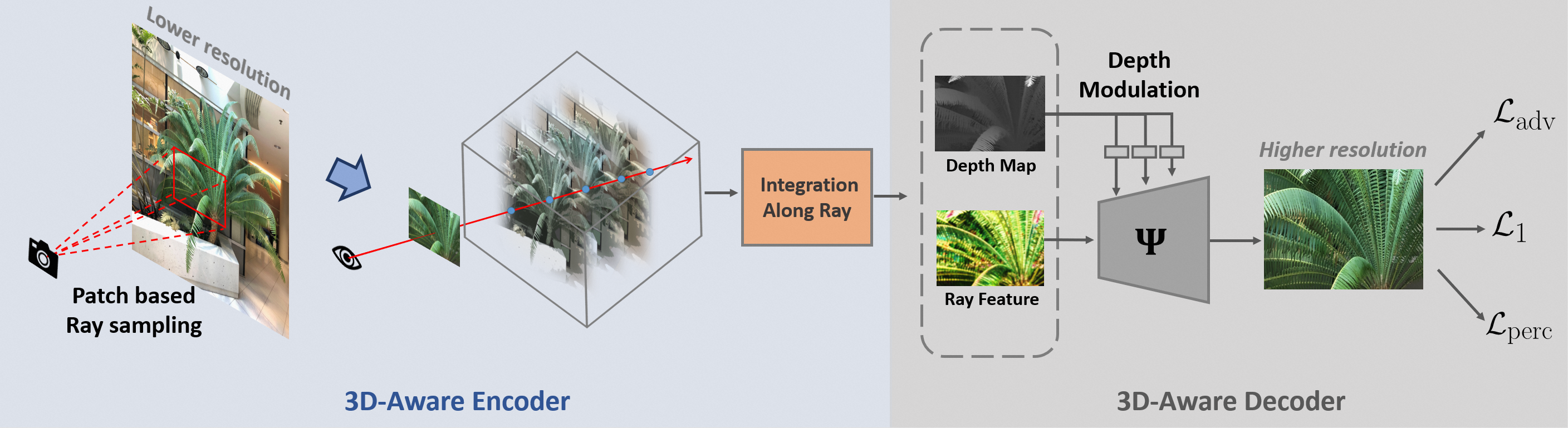
Figure 2: The overall pipeline of 4K-NeRF. Using patch-based ray sampling, we jointly train the 3D-Aware encoder for embedding 3D geometric information in a lower resolution space and the 3D-Aware decoder for realizing rendering enhancement on high-frequency details in the full resolution space.

Ultra-High-Resolution has growing popular as a standard for recording and displaying images and videos, even supported in modern mobile devices. A scene captured in ultra high resolution format typically presents content with incredible details compared to using a relatively lower resolution (e.g, 1K high-definition format) in which the information at a pixel is enlarged by a small patch in extremely high resolution images. Developing techniques for handling such high-frequency details poses challenges for a wide range of tasks in image processing and computer vision. In this paper, we focus on the novel view synthesis task and investigate the potential of realizing high fidelity view synthesis rich in subtle details at ultra high resolution.

Novel view synthesis aims to produce free-view photo-realistic synthesis captured for a scene from a set of viewpoints. Recently, Neural Radiance Fields [24] offer a new methodology for modeling and rendering 3D scenes by virtue of deep neural networks and have demonstrated remarkable success on improving visual quality compared to traditional view interpolation methods [43, 33]. Particularly, a mapping function, instantiated as a deep multilayer perceptron (MLP), is optimized to associate each 3D location given a viewing direction to its corresponding radiance color and volume density, while realizing view-dependent effect requires querying the large network hundreds of times for casting a ray through each pixel. Several following approaches are proposed to improve the method either from the respect of reducing aliasing artifacts on multiple scales [1] or improving training and inference efficiency benefiting from the use of discretized structures [44, 32, 6]. All these methods follow the pixel-wise mechanism despite varying architectures, i.e., rays (or pixels) are regarded individually during training and inference phase. They are typically developed on training views up to 1K resolution. When applying the approaches on ultra-high-resolution scenarios, they would struggle with objectionable blurring artifacts (as shown in Fig. 3) due to insufficient representational ability for capturing fine details.

In this paper, we introduce a novel framework, named 4K-NeRF, building upon the methodology of NeRF-based volume rendering to realize high fidelity view synthesis at 4K ultra-high-resolution. We take the inspiration from the success of convolutional neural networks on traditional super resolution [11]. We expect to boost the representational power of NeRF-based methods by better exploring local correlations between rays.

Specially, the framework is comprised of two components, a 3D-aware encoder and a 3D-aware decoder, as shown in Fig. 2. The encoder encodes geometric properties of a scene effectively in a lower resolution space, forming intermediate ray features and geometry information (i.e., estimated depth) feeding into the decoder. The decoder is capable of recovering high-frequency details by integrating geometry-aware local patterns learned through depth-modulated convolutions in the higher resolution (full-scale) observations. We further introduce a patch-based ray sampling strategy replacing the random sampling in NeRFs, allowing the encoder and the decoder trained jointly with the perception-oriented losses complementing to the conventional pixel-wise MSE loss. Such a joint training facilitates coordinating geometric modelling in the encoder with local context learning in the decoder. Compared to traditional pixel-wise mechanism [24, 32] our method can realize significant enhancement on fine details even with an extreme zoom-in extent (as shown in Fig. 1). Extensive comparison and ablation studies on synthetic and real-world scenes demonstrate the effectiveness of the proposed framework both quantitatively and qualitatively.

2 Related work

Neural Radiance Fields. NeRF [24] formulate a continuous mapping from coordinates to corresponding color and density through MLP via differentiable volume rendering and achieves impressive rendering quality. Some approaches realize significant acceleration on training and rendering speed by virtue of explicit structures, e.g., octree-based structure [45], dense [32] or sparse voxel grids [14, 21, 27, 44] or a hybrid structure [16], radiance maps [13], and tri-planes [6]. Some methods focus on improving the rendering quality of NeRF from different aspects. The works in [1, 2] leverage the insight of mipmap to achieve anti-aliasing. [34, 42] improve representational ability on modelling specular reflections. A series of methods are developed on sparse views, either benefiting from depth prior [10, 28] or taking as input image features extracted from 2D convolutional networks [46, 7]. To the best of our knowledge, our framework is the first to successfully extend NeRF-based paradigm to 4K resolution, proving high-fidelity viewing experience with crystal-clear and high-frequency details.

Novel View Synthesis. Apart from directly approximate a radiance fields for image synthesis, many effort have been done by the research community for view synthesis, mainly representing the 3D scene with the data structure of mesh [29, 15], point cloud [41] and multiplane images [33, 12, 4]. Some recent methods use CNN or transformer to enhance visual quality. IBRNet [36] enables large-scale reasoning with a ray transformer. DeepVoxel [31] takes advantage of both 3D and 2D CNNs to achieve better 3D representation and improve final render quality. EG3D [5] applies a 2D upsample module to increase the resolution of generated faces. GIRAFFE [26] realizes a compositional generative model incorporating with 2D neural rendering via 2D convolutional networks. In contrast, our method realize extremely high-resolution view synthesis by better exploiting geometry-aware local patterns, i.e., enhancing correlation of ray features via depth-modulated convolutions.

High-Resolution Synthesis. The framework is also related to image super-resolution techniques which recover high-resolution images from low-resolution ones. Classical methods are typically derived from strong prior on ideal image degradation type, i.e., downsampling and noisy [11, 17]. These methods investigate gradient propagation in low-level network layers [49, 8] or the balance between distortion and perception [19, 39]. In order to address more complex scenarios, some methods introduce first-order [47, 20] and high-order hybrid degradation modeling [37], and have achieved promising performance on real-world data. All of these super-resolution methods perform on resolving 2D single image. The most related work to ours is NeRF-SR [35], which incorporates super-resolution/sampling into NeRFs. Unlike using a joint training scheme in our framework, the method trains a separate refinement network to super-resolve image patches by using the max-pooled features of relevant patches sampled from higher-resolution references, resulting in less-consistent rendering across viewpoints.

3 Method

3.1 Volumetric Rendering

NeRF realizes view synthesis by learning a continuous mapping function to estimate the color $\mathbf{c}\in\mathbb{R}^{3}$ and the volume density $\sigma\in\mathbb{R}$ of a 3D point position $\mathbf{x}\in\mathbb{R}^{3}$ and a viewing direction $\mathbf{d}\in\mathbb{R}^{3}$, i.e., $\Phi:(\mathbf{x},\mathbf{d})\mapsto(\mathbf{c},\sigma)$. To render an image given camera pose, the expected color $\widehat{\mathbf{C}}(\mathbf{r})$ of a camera ray $\mathbf{r}=\mathbf{o}+t\mathbf{d}$ through the pixel is estimated by sampling a set of points along the ray and integrating their colors to approximate a volumetric rendering integral [22],

$$\widehat{\mathbf{C}}(\mathbf{r})=\sum_{i=1}^{N}T_{i}\cdot\alpha_{i}\cdot\mathbf{c}_{i},$$ (1)

$$\alpha_{i}=1-\exp(-\sigma_{i}\delta_{i}),\quad T_{i}=\prod_{j=1}^{i-1}(1-\alpha_{j}),$$ (2)

where $\alpha_{i}$ denotes the ray termination probability at the point $i$, $\delta_{i}=t_{i+1}-t_{i}$ represents the distance between two adjacent points, and $T_{i}$ indicates the accumulated transmittance when reaching $i$. The mapping function $\Phi$ is instantiated as a MLP. Given the training views with known poses, the model is trained by minimizing the mean squared errors (MSE) between the predicted pixel colors and the ground-truth colors,

$$\mathcal{L}_{\text{MSE}}=\frac{1}{|\mathcal{R}|}\sum_{\mathbf{r}\in\mathcal{R}}\left\|\widehat{\mathbf{C}}(\mathbf{r})-\mathbf{C}(\mathbf{r})\right\|_{2}^{2},$$ (3)

where $\mathcal{R}$ denotes the ray set randomly sampled in each min-batch. The optimization of each point is according to its projection through the rays of different viewpoints. Some variants are distinct from using single large neural networks, by integrating the benefit of explicit structures [27, 21, 44, 32], while all these methods intrinsically learn geometry-aware representations in pixel-wise manner despite architecture difference.

Limitation. Rays (or pixels) are treated independently during training and inference process. The cardinality of the ray set grows quadratically with the increase of image resolution. For an image of 4K ultra high resolution, there exists over 8 million pixels typically presenting richer details and each of which naturally embodies scene content in a finer level than the one on a lower resolution image. If directly using such a pixel-wise training mechanism on extremely high-resolution inputs, these methods may struggle with insufficient representational ability for retaining subtle details, even with increased model capacity (shown in the supplementary materials), which might worsen the issues of lengthy inference with a tremendous MLP or considerable storage cost by using voxel-grid structures with increased volume dimension.

3.2 Overall Framework

To extend conventional NeRF methods to achieve high-quality rendering at ultra high resolutions, one straightforward solution is to first train NeRF models for rendering down-sampled outputs and then train parameterized super-resolution on each view to up-sample them to full scale. However, such a solution would result in obvious artifacts of inconsistent rendering across viewpoint, as local patterns captured in the super-resolution stage lack regularization from holistic geometry (as shown in the ablation study of joint training in 5.5).

In this regard, we develop a simple yet effective framework which first encodes geometric information in a lower resolution space through 3D-Aware Encoder module and recover subtle details in a higher resolution (HR) space via the 3D-Aware Decoder module. The method aims to boost high-frequency details recovery by integrating 3D-aware local correlations learned in the observations.

3.3 3D-Aware Encoder

We instantiate the encoder based on the formulation defined in the DVGO [32], where voxel-grid based representations are learned to encode geometric structure explicitly,

$$\left(\textbf{x},\textbf{V}\right):\left(\mathbb{R}^{3},\mathbb{R}^{N_{c}\times N_{x}\times N_{y}\times N_{z}}\right)\rightarrow\mathbb{R}^{N_{c}},$$ (4)

where $N_{c}$ denotes the channel dimension for density ($N_{c}=1$) and color modality, respectively. For each sampling point, the density is estimated by trilinear interpolation equipped with a softplus activation, i.e., $\sigma=\text{softplus}\left(\text{interp}\left(\textbf{x},\textbf{V}_{d}\right)\right)$. The colors are estimated with a shallow MLP,

$$\mathbf{c} =f_{\text{MLP}}\left(\text{interp}\left(\textbf{x},\textbf{V}_{c}\right),\textbf{x},\textbf{d}\right)$$ (5)

$$=f_{\text{RGB}}\big{(}g_{\theta}(\text{interp}(\textbf{x},\textbf{V}_{c}),\textbf{x},\textbf{d})\big{)},$$

where $g_{\theta}(\cdot)$ extracts volumetric features for color information, and $f_{\text{RGB}}$ denotes the mapping (with one or multiple layers) from the features to RGB images.

The output $\mathbf{g}=g(\theta;\mathbf{x},\mathbf{d})$ denotes the volumetric feature for the point $\mathbf{x}$ with the viewing direction $\mathbf{d}$. We can then get the descriptor for each ray (or pixel) by accumulating the features of sampling points along the ray $\mathbf{r}$ as in Eqn.1 ,

$$\mathbf{f}(\mathbf{r})=\sum_{i=1}^{N}T_{i}\cdot\alpha_{i}\cdot\mathbf{g}_{i}.$$ (6)

For better use of geometric properties embedded in the encoder, we also generate a depth map by estimating the depth along the camera axis for each ray $\mathbf{r}$,

$$M(\mathbf{r})=\sum_{i=1}^{N}T_{i}\cdot\alpha_{i}\cdot t_{i},$$ (7)

where $t_{i}$ denotes the distance of the sampling point $i$ to the camera center as in Eqn.1. The estimated depth map provides a strong guidance for understating the 3D structure of a scene, e.g., nearby pixels on the image plane may be far away in the original 3D space. Assume the spatial dimension is $H^{\prime}\times W^{\prime}$, the formed feature maps $\mathbf{F}_{\text{en}}\in\mathbb{R}^{C^{\prime}\times H^{\prime}\times W^{\prime}}$ and the depth map $\mathbf{M}\in\mathbb{R}^{H^{\prime}\times W^{\prime}}$ are fed into the decoder for pursuing high-fidelity reconstruction of fine details.

3.4 3D-Aware Decoder

The decoder performs view synthesis at a higher spatial dimension $H\times W$ space by training a convolutional neural network $\Psi:\left(\mathbf{F_{\text{en}}},\mathbf{M}\right)\mapsto\mathbf{P}$, where $\mathbf{P}\in\mathbb{R}^{3\times H\times W}$, $H=sH^{\prime}$ and $W=sW^{\prime}$, and $s$ indicates the up-sampling scale. The network is built by stacking several convolutional blocks (with neither non-parametric normalization nor down-sampling operations) interleaved with up-sampling operations. Particularly, instead of simply concatenating the features $\mathbf{F}_{\text{en}}$ and the depth map $\mathbf{M}$, we regard depth signal separately and inject it into every block through a learned transformation to modulate block activation.

Formally, suppose $\mathbf{F}^{k}$ denotes the activation of an intermediate block with the channel dimension $C_{k}$. The depth map $\mathbf{M}$ passes through the transformation (e.g., with $1\times 1$ convolution) to predict scale and bias values with the same dimension $C_{k}$, used to modulate $\mathbf{F}^{k}$ according to:

$$\tilde{\mathbf{F}}^{k}_{i,j}=\gamma_{i,j}^{k}(\mathbf{M})\odot\mathbf{F}^{k}_{i,j}+\beta_{i,j}(\mathbf{M}).$$ (8)

where $\odot$ denotes element-wise product, $i$ and $j$ indicate the spatial position. More detailed descriptions for the network architecture can be founded in the implementation section and supplemental material.

Integrating local information of nearby pixels has proven to be effective for recovering high frequency details in single image super-resolution. Learning local correlation of ray features naturally connects pattern extraction across spacial regions to the underlying 3D geometric structure, and the modulation with depth maps further regularize the learning with geometric guidance.

4 Training

The encoder and the decoder are jointly trained and the overall framework can be trained in a differentiable and end-to-end manner.

Patch-based Ray Sampling. Our method aims to capture spatial information between rays (pixels). Therefore, the random ray sampling strategy used in traditional NeRF methods is unsuitable here. We present a training strategy with patch-based ray sampling to facilitate the capture of spatial dependencies between ray features.

We first split the images of training views into patches $\mathbf{p}$ with the size $N_{p}\times N_{p}$ in order to ensure the sampling probability on pixels are uniform. When the image spatial dimension can not be exactly divided by the patch size, we truncate the patch until edge and obtain a set of training patches. A patch (or multiple patches) is randomly sampled from the set, and the rays casting through the pixels in the patch form the mini-batch of each iteration.

Loss Functions. We found that only using distortion-oriented loss (e.g., MSE, $\ell_{1}$ and Huber loss) as objective tends to produce blurry or over-smoothed visual effects on fine details. In order to solve the problem, we add the adversarial loss and the perceptual loss to regularize fine detail synthesis. The adversarial loss $\mathcal{L}_{\text{adv}}$ is calculated on the predicted image patches via the decoder and training patches through a learnable discriminator which aims to distinguish the distribution of training data and predicted one. The perceptual loss $\mathcal{L}_{\text{perc}}$ estimates the similarity between predicted patches $\hat{\mathbf{p}}$ and Ground-Truth $\mathbf{p}$ in the feature space via a pretrained 19-layer VGG network $\varphi$ [30],

$$\mathcal{L}_{\text{perc}}=\left\|\varphi(\hat{\mathbf{p}})-\varphi(\mathbf{p})\right\|_{2}^{2}.$$ (9)

We use $\ell_{1}$ loss instead of MSE for supervising the reconstruction of high-frequency details,

$$\mathcal{L}_{1}=\frac{1}{N_{p}^{2}}\left|\mathbf{C}({\hat{\mathbf{p}})}-\mathbf{C}(\mathbf{p})\right|.$$ (10)

We add an auxiliary MSE loss to facilitate the training of encoder with down-scaled training views, i.e., the ray features produced by the encoder are fed into an extra fully-connected layer to regress RGB values in the lower-resolution images. The overall training objective is defined as,

$$\mathcal{L}=\lambda_{h}\mathcal{L}_{\text{1}}+\lambda_{a}\mathcal{L}_{\text{adv}}+\lambda_{p}\mathcal{L}_{\text{perc}}+\lambda_{l}\mathcal{L}_{\text{MSE}}^{l}.$$ (11)

where $\lambda_{h}$, $\lambda_{a}$, $\lambda_{p}$ and $\lambda_{l}$ denote the hyper-parameters for weighting the losses.

5 Experiments

5.1 Implementation

3D-Aware Encoder. We use the configuration of DVGO as the default setting for the encoder. Specially, we extract the ray features at the penultimate layer of the MLP (with the channel dimension $64$) following a dimensional reduction layer (with the channel dimension $6$), then the obtained features are fed into the decoder.

3D-Aware Decoder. We employ a residual skip-connected convolutional blocks [39] for the decoder. Specifically, the decoder consists of a backbone with 5 blocks and an up-sampling head to produce full-scale images. We plug the depth modulation module at the end of each block. Detailed architecture can refer to supplemental material.

Training. To facilitate training convergence, in practice we initialize the encoder by pretraining it with 30k iterations following the training setting of DVGO . We then jointly train the encoder and the decoder for 200k iterations with patch size of 64. The loss parameters $\lambda_{h}$, $\lambda_{p}$, $\lambda_{a}$ and $\lambda_{l}$ are respectively set to 1.0, 0.5, 0.02 and 1.0. The learning rates for updating the encoder and the decoder are 1e-4 and 2e-4.

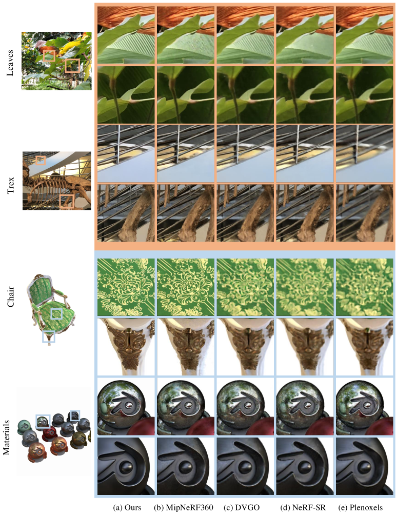
Figure 3: Visual comparison with modern NeRF methods on example scenes from 4K-LLFF and 4K-Synthetic-NeRF. Our method shows significant enhancement on preserving high-frequency details, either with complex geometry or high reflection surface, outperforming all the baseline methods obviously. The figure is better displayed on a high-resolution screen.

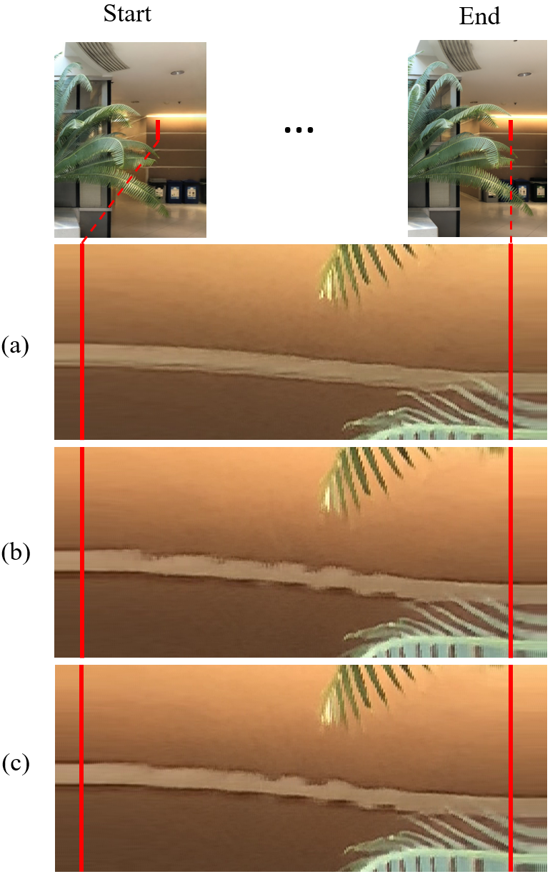
Figure 4: View-consistency visualization. From horizontal view interpolation videos, we extract a short vertical segment pixel at fixed location every frame and stack them horizontally to compare view consistency between (a) full training, (b) w/o depth modulation and (c) w/o joint training.

5.2 Evaluation Metrics

PSNR for evaluating distortion is used as the default metric in NeRF methods, while the metric is insensitive for the artifacts like over-smooth or blurry details, which has been well-analyzed in [3]. We hence evaluate the method with more metrics, including LPIPS [48] and NIQE [25] metrics for assessing perceptual effect, as well as another distortion-oriented metric SSIM [40]. LPIPS is calculated with AlexNet [18].

5.3 Datasets

4K-LLFF. The LLFF dataset [23] provides forward real-world scenes with training views at 4K ultra high resolution. It is composed of 8 forward-facing scenes and different scenes have different numbers of training views, between 20 and 60. Unlike using down-sampled images with 1K resolution in conventional NeRF methods, we use the full scale images ($4032\times 3024$) for training and evaluation.

4K-Synthetic-NeRF. The Synthetic-NeRF dataset [24] consists of the images rendered from 8 synthetic objects at the resolution of $800\times 800$. Each scene contains $100$ training views and the other $200$ testing views. We re-render all the scene at $3200\times 3200$ resolution based the original 3D models, forming the 4K version of the dataset.

5.4 Comparisons

Quantitative evaluation. We first conduct the experiments to compare the method with modern NeRF methods, including Plenoxels [44], DVGO [32], JaxNeRF [9], MipNeRF-360 [2] and NeRF-SR [35] training and evaluating at 4K resolution. The results on 4K-LLFF and 4K-Synthetic-NeRF are respectively shown in Table 1 and Table 2. Our method (training with default loss setting) achieves obvious advantage in the perception metrics (i.e., LPIPS and NIQE) compared to all the baselines. The performance is comparable on the distortion metrics, slightly inferior to some baselines on the real-world scenes of LLFF. To better understand the method, we also provide the result by training a variant with $\mathcal{L}_{1}$ only in the decoder (i.e., without the adversarial and the perception losses) on LLFF, which achieves the best performance on the distortion metrics. Detailed analysis for the loss function can be found in the following ablation studies.

Besides rendering quality metrics, we also provide inference time and training runtime memory as reference for a comprehensive evaluation. Our method achieves compelling performance on both metrics, allowing to render an 4K image within 600 ms. Our method achieves over $10\times$ faster inference with less than half training memory overhead compared to the direct counterpart DVGO.

Qualitative comparison. We provide the visual comparison in Fig. 3. Our method is capable of achieving high-fidelity photo-realistic rendering at such extremely high resolution scenes. The baseline methods show inferior ability on reconstructing subtle details at 4K scenes, incurring details lost or blur, e.g., leaf and chair texture. The visual quality of our method is obviously superior for preserving such complex and high-frequency details, even on the scenes with high reflection surfaces.

	Perception metrics		Distortion metrics
Methods	LPIPS $\downarrow$	NIQE$\downarrow$	PSNR$\uparrow$	SSIM$\uparrow$	Inference time (s)$\downarrow$	Runtime memory (GB)$\downarrow$
Plenoxels	0.48	8.86	24.56	0.775	1.88	29.1
DVGO	0.44	7.89	25.13	0.779	5.68	58.6
JaxNeRF	0.42	7.03	25.37	0.773	134.62	77.8
MipNeRF-360	0.37	6.31	25.34	0.789	51.38	78.1
NeRF-SR	0.52	9.26	24.15	0.754	129.19	46.7
Ours-$\mathcal{L}_{1}$	0.41	7.45	25.44	0.793	0.58	14.9
Ours	0.21	4.75	24.71	0.767	0.58	14.9

Table 1: Quantitative comparison with modern NeRF methods on 4K-LLFF dataset. LPIPS is calculated with AlexNet. Our method ranks first on LPIPS and NIQE and achieve a comparable distortion performance. The variant of training only with $\ell_{1}$ loss can achieve better performance on distortion metrics. Our method also show benefits on inference speed and run-time memory overhead.

				Memory
Methods	LPIPS$\downarrow$	PSNR$\uparrow$	SSIM$\uparrow$	(GB)$\downarrow$
Plenoxels	0.097	29.45	0.937	10
DVGO	0.097	29.61	0.938	48.4
JaxNeRF	0.102	29.98	0.928	77.7
MipNeRF-360	0.075	31.32	0.948	77.2
NeRF-SR	0.139	28.39	0.904	46.7
Ours-$\mathcal{L}_{1}$	0.063	30.71	0.952	21.4

Table 2: Quantitative comparison on 4K-Synthetic-NeRF.

5.5 Ablation studies

Joint training. In order to better investigate the effect of joint training, we compare it to the setting of training the pair of encoder and decoder separately, i.e., fully train the encoder and then train the decoder without propagating gradient back to the encoder. We splice a clip of pixel strips at a fixed position in each frame of the rendered video and show the result in Fig. 4. The margin of texture jitter is a strong indicator for judging consistency extent across view. Compared to joint training, there exists obvious texture jitter via separate training, showing that the rendering results with joint training are more view-consistent.

Depth modulation. We integrate the explicit geometrical guidance into the decoder through the use of estimated depth, and validate its effect via the study without depth injection. Modulation with depth can benefit rendering results with more view consistency compared to without depth (in Fig. 4). It is helpful for improving rendering quality (as shown in Table 3) , especially for the scene details close to view plane, as shown in Fig. 5, which is more consistent with human vision.

Loss function. Using multiple losses would encourage the learning of discriminative patterns towards different aspects. As shown in Fig. 5, the regularization of the perception loss and the adversarial loss enables apparent visual quality improvement with richer and delicate textures (e.g., sharp leaf and screw thread) compared to using the distortion loss $\mathcal{L}_{1}$ only. Regularizing only with $\mathcal{L}_{1}$ may result in blurry and over-smooth artifacts on fine details although it can reach a higher value on the distortion metrics PSNR and SSIM. We also empirically found the adversarial loss shows better ability for recovering radiance compared to the perception loss.

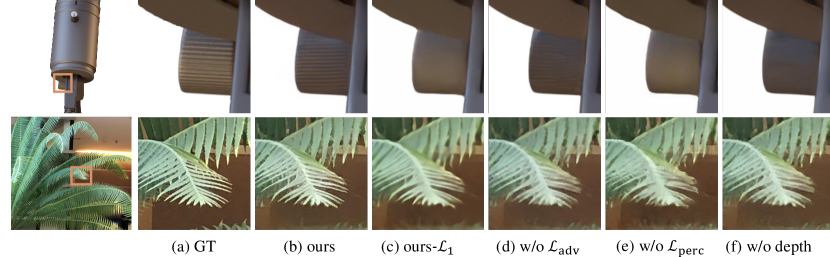
Figure 5: Visual results of ablation studies on loss functions and depth modulation on the scenes of “Mic” and “Fern”.

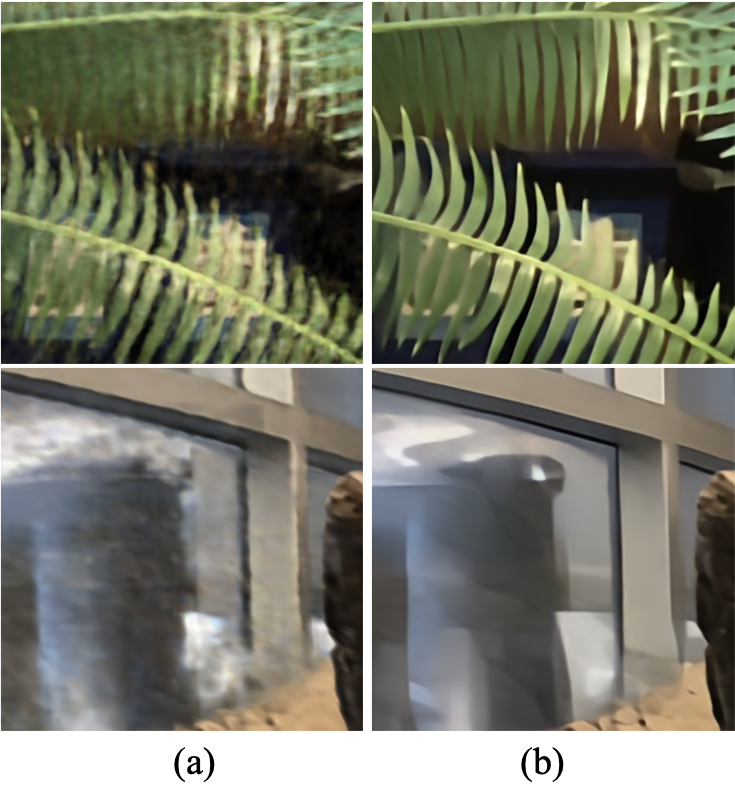
Figure 6: Qualitative comparison of baseline TensoRF (a) and our method with TensoRF-based Encoder (b).

Method	LPIPS$\downarrow$	NIQE$\downarrow$	PSNR$\uparrow$	SSIM$\uparrow$
ours	0.162	4.20	23.49	0.771
ours-$\mathcal{L}_{\text{1}}$	0.353	6.37	23.69	0.778
w/o depth	0.189	4.61	23.36	0.754
w/o $\mathcal{L}_{\text{adv}}$	0.205	6.89	23.39	0.759
w/o $\mathcal{L}_{\text{perc}}$	0.241	4.51	23.31	0.764

Table 3: Ablation study of losses and depth on “Fern” scene.

Encoder Backbone. The base encoder can be instantiated with different NeRF-based architectures. In order to assess the generalization of our framework, we conduct the experiment by using TensoRF [6] instead of DVGO as the encoder base. The qualitative and quantitative results are shown in Fig. 6 and Table. 4. Clear improvements are achieved on both evaluation metrics and visual qualities, showing that our method can boost rendering quality on fine details and reduce blurry artifacts even on challenging transparent/translucent objects.

Other ablation studies, such as the impact of decoder capacity and patch size, are shown in supplementary materials.

5.6 Limitation and Future Work

Our method can recover high-frequency details well at ultra high-resolution scenes and show strong adaptability to reflection and translucency. However, we empirically found adding perception loss may happen to confine the recovery of highlight colors (e.g., slight color aberration on the button shown in Fig.4 top row). This may be alleviated by tuning the loss parameters in an elaborate manner or incorporating more meta information (e.g., ray direction, normal map and reflectance) into the decoder learning. The training time of our method is relatively long due to training the decoder with convolutional networks and the discriminator in the adversarial loss. As a future work we will consider taking advantage of pre-training models from image super-resolution tasks or extending the generalization of decoder (associated with fast fine-tuning) to reduce per-scene training cost.

Scene	Method	LPIPS $\downarrow$	NIQE $\downarrow$	PSNR $\uparrow$
	TensoRF	0.464	7.172	23.33
Fern	Ours	0.342	6.089	23.27
	TensoRF	0.452	7.051	26.19
Horns	Ours	0.387	6.276	26.72

Table 4: 3D-Aware Encoder based on TensoRF.

6 Conclusion

In this paper, we explored the ability of NeRF methods on modelling fine details of 3D scenes and proposed a novel framework to boost its representational power on recovering subtle details at 4K ultra high resolutions. A pair of encoder-decoder modules are introduced to take better use of geometric properties for realizing impressive rendering quality on complex and high-frequency details, by virtue of local correlation captured from geometry-aware features. Patch-based sampling allows the training to integrate the supervision from perception-oriented regularization beyond pixel-level mechanism. We expect to investigate the effect of enhancing ray correlation, especially incorporated with the success of existing perception and generative methods, on pursing high-fidelity 3D scene modelling and manipulation as well as extending to dynamic scenes as future directions.

4K-NeRF: High Fidelity Neural Radiance Fields at Ultra High Resolutions
Appendix

Appendix A Details of Model Structure

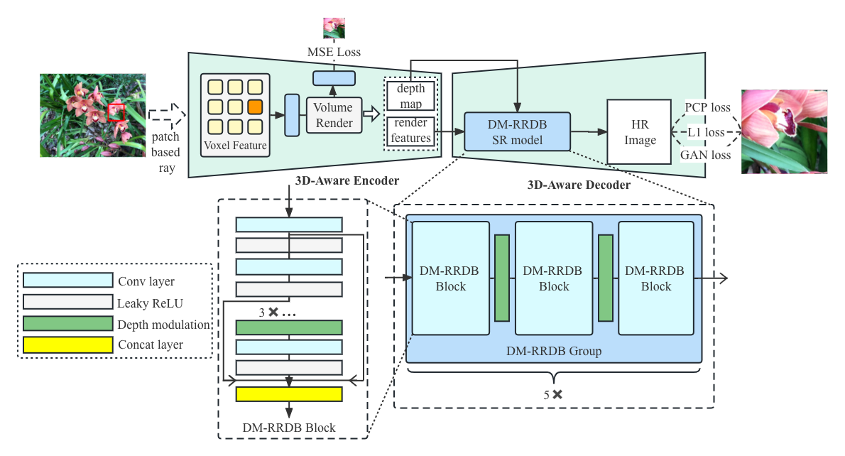
Figure 7: The scheme of 4K-NeRF in detail.

We use the default configuration of DVGO [32] as the encoder setting in the experiments. Specifically, the size of voxels is $384\times 384\times 256$, and each voxel contains a density value representing geometry and a 12-dimensional color feature followed by a MLP. We extract ray features from the MLP with the channel dimension 64 following a dimensional reduction layer with the channel dimension 6. The encoder is trained on the resolution $1008\times 756$.

The illustration of the 4K-NeRF structure is shown in Fig. 7. The decoder consists of 5 residual-in-residual dense modules (RRDB) [39, 38] with depth modulation (DM-) as well as one super-resolution head. Each module is comprised of three DM-RRDB blocks interleaved with depth modulation units. We also insert a depth modulation unit for each DM-RRDB block. More detailed configuration can refer to the network configuration provided in the source code. Resolution increase performs in the super-resolution head by stacking two convolutional layers interleaved with $2\times$ bi-linear upsamling operation.

Patch Size	LPIPS$\downarrow$	NIQE$\downarrow$	PSNR$\uparrow$	SSIM$\uparrow$	Training time(min)$\downarrow$	Runtime Memory(GB)$\downarrow$
32	0.24	5.93	24.80	0.767	240	13.8
64	0.21	4.75	24.71	0.767	300	14.9
128	0.18	5.33	24.85	0.760	600	17.6
256	0.19	5.27	24.70	0.757	780	29.1

Table 5: Ablation study of different patch size on 4K-LLFF.

				Memory
Dataset	Method	LPIPS$\downarrow$	PSNR$\uparrow$	(GB)$\downarrow$
	DVGO	0.44	25.13	58.6
	DVGOlarge	0.39	25.53	72.6
LLFF	Ours-$\mathcal{L}_{1}$	0.41	25.44	14.9
	Ours	0.21	24.71	14.9
	DVGO	0.10	29.61	48.4
	DVGOlarge	0.07	31.42	77.2
4K-SYN	Ours-$\mathcal{L}_{1}$	0.06	30.71	21.4
	Ours	0.03	29.12	21.4

Table 6: Quantitative comparison on 4K-LLFF and 4K-Synthetic-NeRF datasets among DVGO, DVGO_large and ours.

Decoder setting	LPIPS$\downarrow$	NIQE$\downarrow$	PSNR$\uparrow$	SSIM$\uparrow$	Training time$\downarrow$	Inference time$\downarrow$	Parameters
Large (5B64C)	0.207	4.75	24.71	0.767	300 min	0.58 s	4.0 MB
Medium (3B64C)	0.216	5.12	24.47	0.759	255 min	0.47 s	2.4 MB
Small (1B64C)	0.223	5.20	24.30	0.761	154 min	0.31 s	0.9 MB

Table 7: Ablation study of different decoder size in 4K-LLFF datasets.

Appendix B More Descriptions on Evaluation Metrics

Existing NeRF methods are typically supervised by pixel-level MSE loss and estimated by its direct counterpart PSNR metric. However, only using pixel-level loss is intractable to estimate problems like over-smooth details and blurry visual artifacts. These issues have been well analyzed and explained in detail in the papers [3, 48], revealing the relation between perceptual quality and the degree of distortion. Distortion-oriented metrics (such as PSNR) can be treated as a visual lower bound, ensuring that semantic content in the image is consistent when reaching a certain level. The perceptual effects towards human vision, such as texture details and sharpness, can be measured by virtue of perception-oriented metrics, e.g., LPIPS. PSNR may be inconsistent with visual quality estimated by human eyes. This phenomenon is often more pronounced in ultra-high-resolution videos. Therefore, to quantify and compare the results more reasonably, we use LPIPS and NIQE as evaluation metrics besides PSNR. LPIPS and PSNR are calculated based on test ground-truth views (whose number is limited). As NIQE is a GT-free metric, we calculate across frames of rendered videos given camera trace to better assess cross-view quality.

Appendix C More Ablation Studies

The impact of Patch Size. We trained the model with the patches of four sizes and the qualitative results are shown in Table 5. The method can achieve a comparable rendering quality across different patch sizes except using a relatively small patch size ($32\times 32$). It may be less effective for capturing ray correlations from a restricted neighbouring context, resulting in inferior performance on perception metrics. On the other hand, using a larger patch size requires longer training to convergence as well as memory cost. Therefore we recommend choosing a moderate patch size (between 64 and 128), and used 64 by default in the experiments.

The impact of decoder capacity. We conduct the ablation study on decoder capacity with the following three levels, “small”, “medium” and “large”. The comparison results are shown in Table 7. Training a larger decoder costs longer while it shows better ability on improving visual quality. As the core motivation of the work is pursuing high-fidelity rendering, we use the large setting by default while it can achieve a trade-off between rendering quality and other performance metrics (e.g., training cost) by adjusting the decoder capacity.

Directly Scaling Up baseline. We further investigate the ability of expanding traditional NeRF models to a larger capacity, and compare it with our method. We scale up the direct counterpart DVOG, named as DVGO_large, by significantly increasing its model capacity up to running-time memory limit, i.e., increasing the number of MLP channels from 64 to 128, doubling the number of training epochs and expanding the dimension of voxel grids from $384\times 384\times 256$ to $1200\times 1000\times 256$ on the 4K-LLFF dataset and from $160^{3}$ to $640^{3}$ on the 4K-Synthetic-NeRF dataset. The qualitative and visual comparison among DVGO, DVGO_large and ours are shown in Table. 6, Fig. 8. Our method shows obvious improvement compared to DVGO${}_{\text{large}}$ on visually detail recovery as well as the value of perception metric. We also found that compared to the standard setting of DVGO, the large variant sometimes exist more significant artifacts, e.g., cluttered textures and lack of leaves. In contrast, our method can achieve consistent enhancement on visual quality, especially for high-frequency details.

Appendix D Detailed Results

We present detailed results for each scene on the 4K-LLFF and 4K-Synthetic-NeRF datasets in Tables 8. In addition, we provide rendered videos on four representative scenes (“Fern”, “Horns”, “Drums” and “Mic”) for better illustrating the superiority of our method on visual quality of 4K scenes, which we recommend to watch on the 4K ultra-high-resolution display.

Scene	Method	Perception metrics		Distortion metrics		Inference time	Cache memory
		LPIPS $\downarrow$	NIQE $\downarrow$	PSNR $\uparrow$	SSIM $\uparrow$	(s) $\downarrow$	(GB) $\downarrow$
	Plenoxels	0.456	7.721	23.842	0.772	2.3	32.8
	DVGO	0.424	6.910	23.741	0.771	6.2	20.1
	JaxNeRF	0.399	5.623	23.470	0.758	134.7	77.8
	MipNeRF-360	0.348	5.229	23.867	0.786	51.3	78.1
	NeRF-SR	0.516	7.362	22.893	0.735	129.6	46.7
	Ours	0.190	4.201	23.494	0.771	0.3	11.8
Fern	Ours-$\mathcal{L}_{1}$	0.353	6.377	23.691	0.778	0.3	11.8

Scene	Method	Perception metrics		Distortion metrics		Inference time	Cache memory
		LPIPS $\downarrow$	NIQE $\downarrow$	PSNR $\uparrow$	SSIM $\uparrow$	(s) $\downarrow$	(GB) $\downarrow$
	Plenoxels	0.516	10.42	26.103	0.811	2.5	29.3
	DVGO	0.500	9.964	26.857	0.812	5.6	26.5
	JaxNeRF	0.489	9.308	26.783	0.806	134.7	77.8
	MipNeRF-360	0.437	7.824	27.119	0.812	51.3	78.1
	NeRF-SR	0.556	11.07	25.578	0.784	129.6	46.7
	Ours	0.235	5.525	26.454	0.792	0.27	14.2
Flower	Ours-$\mathcal{L}_{1}$	0.493	9.514	26.865	0.820	0.27	14.2

Scene	Method	Perception metrics		Distortion metrics		Inference time	Cache memory
		LPIPS $\downarrow$	NIQE $\downarrow$	PSNR $\uparrow$	SSIM $\uparrow$	(s) $\downarrow$	(GB) $\downarrow$
	Plenoxels	0.491	9.919	28.852	0.860	2.4	30.1
	DVGO	0.397	8.766	29.438	0.864	5.3	30.7
	JaxNeRF	0.336	7.737	30.210	0.869	134.7	77.8
	MipNeRF-360	0.314	7.472	30.169	0.873	51.3	78.1
	NeRF-SR	0.517	9.637	28.719	0.859	129.6	46.7
	Ours	0.197	4.857	28.120	0.846	0.25	15.3
Fortress	Ours-$\mathcal{L}_{1}$	0.404	8.320	29.853	0.876	0.25	15.3

Scene	Method	Perception metrics		Distortion metrics		Inference time	Cache memory
		LPIPS $\downarrow$	NIQE $\downarrow$	PSNR $\uparrow$	SSIM $\uparrow$	(s) $\downarrow$	(GB) $\downarrow$
	Plenoxels	0.510	8.298	24.743	0.756	2.3	31.0
	DVGO	0.462	7.053	25.632	0.760	5.4	40.8
	JaxNeRF	0.430	5.945	26.127	0.770	134.7	77.8
	MipNeRF-360	0.371	5.172	26.220	0.790	51.3	78.1
	NeRF-SR	0.553	9.758	23.694	0.743	129.6	46.7
	Ours	0.191	4.439	25.066	0.742	0.29	18.8
Horns	Ours-$\mathcal{L}_{1}$	0.399	6.241	26.336	0.794	0.29	18.8

Scene	Method	Perception metrics		Distortion metrics		Inference time	Cache memory
		LPIPS $\downarrow$	NIQE $\downarrow$	PSNR $\uparrow$	SSIM $\uparrow$	(s) $\downarrow$	(GB) $\downarrow$
	Plenoxels	0.520	7.749	20.028	0.661	1.0	23.3
	DVGO	0.511	7.388	20.220	0.656	5.7	22.6
	JaxNeRF	0.536	6.942	19.781	0.617	134.7	77.8
	MipNeRF-360	0.427	6.078	19.835	0.660	51.3	78.1
	NeRF-SR	0.559	8.167	19.033	0.604	129.6	46.7
	Ours	0.227	4.367	19.781	0.648	0.25	13.4
Leaves	Ours-$\mathcal{L}_{1}$	0.461	7.075	19.819	0.665	0.25	13.4

Scene	Method	Perception metrics		Distortion metrics		Inference time	Cache memory
		LPIPS $\downarrow$	NIQE $\downarrow$	PSNR $\uparrow$	SSIM $\uparrow$	(s) $\downarrow$	(GB) $\downarrow$
	Plenoxels	0.575	9.150	19.874	0.670	2.1	35.3
	DVGO	0.539	8.112	20.098	0.670	6.1	22.5
	JaxNeRF	0.549	7.872	19.649	0.643	134.7	77.8
	MipNeRF-360	0.482	6.880	19.511	0.662	51.3	78.1
	NeRF-SR	0.594	8.973	19.432	0.637	129.6	46.7
	Ours	0.236	5.203	20.005	0.649	0.32	12.5
Orchids	Ours-$\mathcal{L}_{1}$	0.523	7.649	19.557	0.670	0.32	12.5

Scene	Method	Perception metrics		Distortion metrics		Inference time	Cache memory
		LPIPS $\downarrow$	NIQE $\downarrow$	PSNR $\uparrow$	SSIM $\uparrow$	(s) $\downarrow$	(GB) $\downarrow$
	Plenoxels	0.392	9.038	28.133	0.884	2.7	20.5
	DVGO	0.357	7.979	29.554	0.893	5.4	30.3
	JaxNeRF	0.317	6.744	31.114	0.908	134.7	77.8
	MipNeRF-360	0.309	6.614	30.687	0.908	51.3	78.1
	NeRF-SR	0.407	9.316	29.369	0.891	129.6	46.7
	Ours	0.187	4.724	29.620	0.893	0.27	15.3
Room	Ours-$\mathcal{L}_{1}$	0.304	7.732	31.147	0.912	0.27	15.3

Scene	Method	Perception metrics		Distortion metrics		Inference time	Cache memory
		LPIPS $\downarrow$	NIQE $\downarrow$	PSNR $\uparrow$	SSIM $\uparrow$	(s) $\downarrow$	(GB) $\downarrow$
	Plenoxels	0.409	8.584	24.896	0.792	2.8	30.8
	DVGO	0.356	6.985	25.512	0.805	5.7	37.4
	JaxNeRF	0.335	6.030	25.839	0.814	134.7	77.8
	MipNeRF-360	0.296	5.176	25.312	0.828	51.3	78.1
	NeRF-SR	0.454	9.857	24.230	0.782	129.6	46.7
	Ours	0.193	4.672	25.121	0.796	0.26	18.0
T-rex	Ours-$\mathcal{L}_{1}$	0.324	6.716	26.276	0.834	0.26	18.0

Table 8: Detailed results on 4K-LLFF dataset.

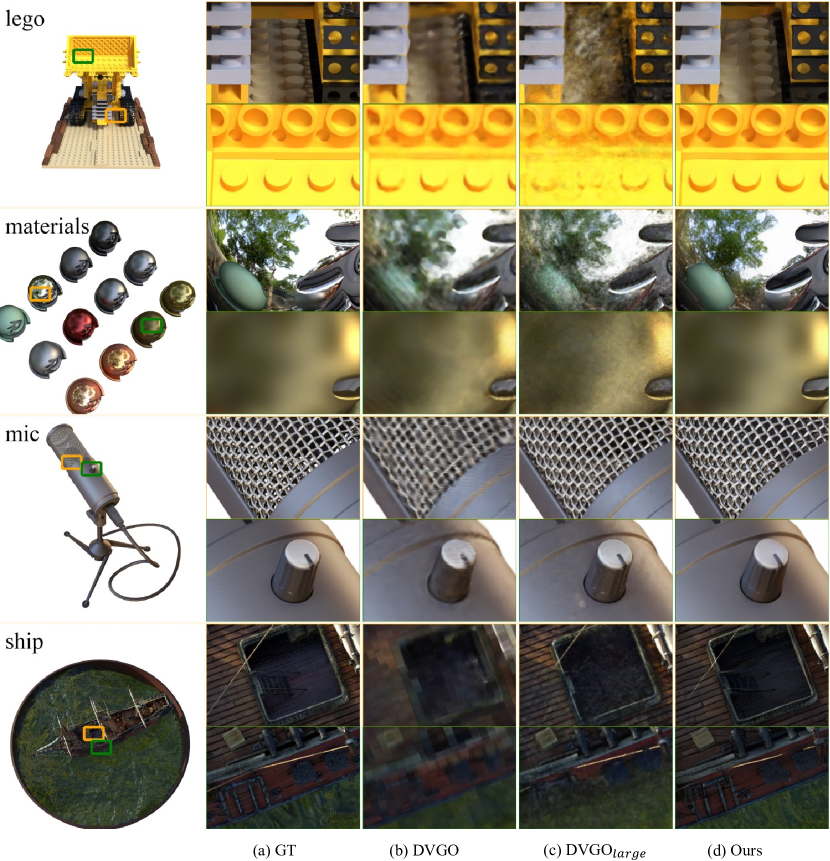
Figure 8: Visual comparison with all kinds of baseline methods on each scenes from 4K-Synthetic-NeRF. Our method shows significant enhancement on preserving high-frequency details, either with complex geometry or high reflection surface, outperforming DVGO and its variant obviously.

References

- [1] Jonathan T. Barron, Ben Mildenhall, Matthew Tancik, Peter Hedman, Ricardo Martin-Brualla, and Pratul P. Srinivasan. Mip-nerf: A multiscale representation for anti-aliasing neural radiance fields. arXiv: Computer Vision and Pattern Recognition, 2021.
- [2] Jonathan T Barron, Ben Mildenhall, Dor Verbin, Pratul P Srinivasan, and Peter Hedman. Mip-nerf 360: Unbounded anti-aliased neural radiance fields. In Proceedings of the IEEE/CVF Conference on Computer Vision and Pattern Recognition, pages 5470–5479, 2022.
- [3] Yochai Blau and Tomer Michaeli. The perception-distortion tradeoff. In Proceedings of the IEEE conference on computer vision and pattern recognition, pages 6228–6237, 2018.
- [4] Michael Broxton, John Flynn, Ryan Overbeck, Daniel Erickson, Peter Hedman, Matthew DuVall, Jason Dourgarian, Jay Busch, Matt Whalen, and Paul Debevec. Immersive light field video with a layered mesh representation. ACM Transactions on Graphics, 2020.
- [5] Eric R. Chan, Connor Z. Lin, Matthew A. Chan, Koki Nagano, Boxiao Pan, Shalini De Mello, Orazio Gallo, Leonidas Guibas, Jonathan Tremblay, Sameh Khamis, Tero Karras, and Gordon Wetzstein. Efficient geometry-aware 3D generative adversarial networks. In arXiv, 2021.
- [6] Anpei Chen, Zexiang Xu, Andreas Geiger, Jingyi Yu, and Hao Su. Tensorf: Tensorial radiance fields. In In Proceedings of the European Conference on Computer Vision, 2022.
- [7] Anpei Chen, Zexiang Xu, Fuqiang Zhao, Xiaoshuai Zhang, Fanbo Xiang, Jingyi Yu, and Hao Su. Mvsnerf: Fast generalizable radiance field reconstruction from multi-view stereo. In International Conference on Computer Vision, 2021.
- [8] Tao Dai, Jianrui Cai, Yongbing Zhang, Shu-Tao Xia, and Lei Zhang. Second-order attention network for single image super-resolution. In Proceedings of the IEEE/CVF conference on computer vision and pattern recognition, pages 11065–11074, 2019.
- [9] Boyang Deng, Jonathan T. Barron, and Pratul P. Srinivasan. JaxNeRF: an efficient JAX implementation of NeRF. https://github.com/google-research/google-research/tree/master/jaxnerf, 2020.
- [10] Kangle Deng, Andrew Liu, Jun-Yan Zhu, and Deva Ramanan. Depth-supervised nerf: Fewer views and faster training for free. In Proceedings of the IEEE/CVF Conference on Computer Vision and Pattern Recognition, pages 12882–12891, 2022.
- [11] Chao Dong, Chen Change Loy, Kaiming He, and Xiaoou Tang. Image super-resolution using deep convolutional networks. IEEE transactions on pattern analysis and machine intelligence, 38(2):295–307, 2015.
- [12] John Flynn, Michael Broxton, Paul Debevec, Matthew DuVall, Graham Fyffe, Ryan Overbeck, Noah Snavely, and Richard Tucker. Deepview: View synthesis with learned gradient descent. Proceedings of the IEEE/CVF International Conference on Computer Vision, 2019.
- [13] Stephan J Garbin, Marek Kowalski, Matthew Johnson, Jamie Shotton, and Julien Valentin. Fastnerf: High-fidelity neural rendering at 200fps. In Proceedings of the IEEE/CVF International Conference on Computer Vision, pages 14346–14355, 2021.
- [14] Peter Hedman, Pratul P. Srinivasan, Ben Mildenhall, Jonathan T. Barron, and Paul E. Debevec. Baking neural radiance fields for real-time view synthesis. In Proceedings of the IEEE/CVF International Conference on Computer Vision, 2021.
- [15] Ronghang Hu, Nikhila Ravi, Alexander C Berg, and Deepak Pathak. Worldsheet: Wrapping the world in a 3d sheet for view synthesis from a single image. In Proceedings of the IEEE/CVF International Conference on Computer Vision, pages 12528–12537, 2021.
- [16] Tao Hu, Shu Liu, Yilun Chen, Tiancheng Shen, and Jiaya Jia. Efficientnerf efficient neural radiance fields. In Proceedings of the IEEE/CVF Conference on Computer Vision and Pattern Recognition, pages 12902–12911, 2022.
- [17] Xiaozhong Ji, Yun Cao, Ying Tai, Chengjie Wang, Jilin Li, and Feiyue Huang. Real-world super-resolution via kernel estimation and noise injection. In proceedings of the IEEE/CVF conference on computer vision and pattern recognition workshops, pages 466–467, 2020.
- [18] Alex Krizhevsky, Ilya Sutskever, and Geoffrey E Hinton. Imagenet classification with deep convolutional neural networks. In Advances in Neural Information Processing Systems, 2012.
- [19] Christian Ledig, Lucas Theis, Ferenc Huszár, Jose Caballero, Andrew Cunningham, Alejandro Acosta, Andrew Aitken, Alykhan Tejani, Johannes Totz, Zehan Wang, et al. Photo-realistic single image super-resolution using a generative adversarial network. In Proceedings of the IEEE conference on computer vision and pattern recognition, pages 4681–4690, 2017.
- [20] Jingyun Liang, Jiezhang Cao, Guolei Sun, Kai Zhang, Luc Van Gool, and Radu Timofte. Swinir: Image restoration using swin transformer. In Proceedings of the IEEE/CVF International Conference on Computer Vision, pages 1833–1844, 2021.
- [21] Lingjie Liu, Jiatao Gu, Kyaw Zaw Lin, Tat-Seng Chua, and Christian Theobalt. Neural sparse voxel fields. In Advances in Neural Information Processing Systems, 2020.
- [22] Nelson L. Max. Optical models for direct volume rendering. IEEE Trans. Vis. Comput. Graph., 1995.
- [23] Ben Mildenhall, Pratul P. Srinivasan, Rodrigo Ortiz-Cayon, Nima Khademi Kalantari, Ravi Ramamoorthi, Ren Ng, and Abhishek Kar. Local light field fusion: Practical view synthesis with prescriptive sampling guidelines. ACM Transactions on Graphics, 2019.
- [24] Ben Mildenhall, Pratul P. Srinivasan, Matthew Tancik, Jonathan T. Barron, Ravi Ramamoorthi, and Ren Ng. Nerf: Representing scenes as neural radiance fields for view synthesis. In In Proceedings of the European Conference on Computer Vision, 2020.
- [25] Anish Mittal, Rajiv Soundararajan, and Alan C Bovik. Making a “completely blind” image quality analyzer. IEEE Signal processing letters, 20(3):209–212, 2012.
- [26] Michael Niemeyer and Andreas Geiger. Giraffe: Representing scenes as compositional generative neural feature fields. In Proceedings of the IEEE/CVF Conference on Computer Vision and Pattern Recognition, 2021.
- [27] Christian Reiser, Songyou Peng, Yiyi Liao, and Andreas Geiger. Kilonerf: Speeding up neural radiance fields with thousands of tiny mlps. In Proceedings of the IEEE/CVF International Conference on Computer Vision, pages 14335–14345, 2021.
- [28] Barbara Roessle, Jonathan T Barron, Ben Mildenhall, Pratul P Srinivasan, and Matthias Nießner. Dense depth priors for neural radiance fields from sparse input views. In Proceedings of the IEEE/CVF Conference on Computer Vision and Pattern Recognition, pages 12892–12901, 2022.
- [29] Meng-Li Shih, Shih-Yang Su, Johannes Kopf, and Jia-Bin Huang. 3d photography using context-aware layered depth inpainting. In Proceedings of the IEEE/CVF Conference on Computer Vision and Pattern Recognition, pages 8028–8038, 2020.
- [30] Karen Simonyan and Andrew Zisserman. Very deep convolutional networks for large-scale image recognition. In International Conference on Learning Representations, 2015.
- [31] Vincent Sitzmann, Justus Thies, Felix Heide, Matthias Nießner, Gordon Wetzstein, and Michael Zollhöfer. Deepvoxels: Learning persistent 3d feature embeddings. In Computer Vision and Pattern Recognition, 2019.
- [32] Cheng Sun, Min Sun, and Hwann-Tzong Chen. Direct voxel grid optimization: Super-fast convergence for radiance fields reconstruction. In Proceedings of the IEEE/CVF Conference on Computer Vision and Pattern Recognition, pages 5459–5469, 2022.
- [33] Richard Tucker and Noah Snavely. Single-view view synthesis with multiplane images. In Proceedings of the IEEE/CVF Conference on Computer Vision and Pattern Recognition, pages 551–560, 2020.
- [34] Dor Verbin, Peter Hedman, Ben Mildenhall, Todd Zickler, Jonathan T. Barron, and Pratul P. Srinivasan. Ref-NeRF: Structured view-dependent appearance for neural radiance fields. Proceedings of the IEEE/CVF International Conference on Computer Vision, 2022.
- [35] Chen Wang, Xian Wu, Yuan-Chen Guo, Song-Hai Zhang, Yu-Wing Tai, and Shi-Min Hu. Nerf-sr: High quality neural radiance fields using supersampling. In Proceedings of the 30th ACM International Conference on Multimedia, pages 6445–6454, 2022.
- [36] Qianqian Wang, Zhicheng Wang, Kyle Genova, Pratul P. Srinivasan, Howard Zhou, Jonathan T. Barron, Ricardo Martin-Brualla, Noah Snavely, and Thomas Funkhouser. Ibrnet: Learning multi-view image-based rendering. In Computer Vision and Pattern Recognition, 2021.
- [37] Xintao Wang, Liangbin Xie, Chao Dong, and Ying Shan. Real-esrgan: Training real-world blind super-resolution with pure synthetic data. In Proceedings of the IEEE/CVF International Conference on Computer Vision, pages 1905–1914, 2021.
- [38] Xintao Wang, Liangbin Xie, Ke Yu, Kelvin C.K. Chan, Chen Change Loy, and Chao Dong. BasicSR: Open source image and video restoration toolbox. https://github.com/XPixelGroup/BasicSR, 2022.
- [39] Xintao Wang, Ke Yu, Shixiang Wu, Jinjin Gu, Yihao Liu, Chao Dong, Yu Qiao, and Chen Change Loy. Esrgan: Enhanced super-resolution generative adversarial networks. In Proceedings of the European conference on computer vision (ECCV) workshops, pages 0–0, 2018.
- [40] Zhou Wang, Alan C. Bovik, Hamid R. Sheikh, and Eero P. Simoncelli. Image quality assessment: from error visibility to structural similarity. IEEE transactions on image processing, 2004.
- [41] Olivia Wiles, Georgia Gkioxari, Richard Szeliski, and Justin Johnson. Synsin: End-to-end view synthesis from a single image. In Proceedings of the IEEE/CVF Conference on Computer Vision and Pattern Recognition, pages 7467–7477, 2020.
- [42] Suttisak Wizadwongsa, Pakkapon Phongthawee, Jiraphon Yenphraphai, and Supasorn Suwajanakorn. Nex: Real-time view synthesis with neural basis expansion. In Proceedings of the IEEE/CVF International Conference on Computer Vision, 2021.
- [43] Yao Yao, Zixin Luo, Shiwei Li, Tian Fang, and Long Quan. Mvsnet: Depth inference for unstructured multi-view stereo. In ECCV, 2018.
- [44] Alex Yu, Sara Fridovich-Keil, Matthew Tancik, Qinhong Chen, Benjamin Recht, and Angjoo Kanazawa. Plenoxels: Radiance fields without neural networks. arXiv preprint arXiv:2112.05131, 2021.
- [45] Alex Yu, Ruilong Li, Matthew Tancik, Hao Li, Ren Ng, and Angjoo Kanazawa. PlenOctrees for real-time rendering of neural radiance fields. In Proceedings of the IEEE/CVF International Conference on Computer Vision, 2021.
- [46] Alex Yu, Vickie Ye, Matthew Tancik, and Angjoo Kanazawa. pixelnerf: Neural radiance fields from one or few images. In Proceedings of the IEEE/CVF Conference on Computer Vision and Pattern Recognition, pages 4578–4587, 2021.
- [47] Kai Zhang, Jingyun Liang, Luc Van Gool, and Radu Timofte. Designing a practical degradation model for deep blind image super-resolution. In Proceedings of the IEEE/CVF International Conference on Computer Vision, pages 4791–4800, 2021.
- [48] Richard Zhang, Phillip Isola, Alexei A Efros, Eli Shechtman, and Oliver Wang. The unreasonable effectiveness of deep features as a perceptual metric. In Proceedings of the IEEE conference on computer vision and pattern recognition, pages 586–595, 2018.
- [49] Yulun Zhang, Kunpeng Li, Kai Li, Lichen Wang, Bineng Zhong, and Yun Fu. Image super-resolution using very deep residual channel attention networks. In Proceedings of the European conference on computer vision (ECCV), pages 286–301, 2018.