Dynamic Test-Time Augmentation via Differentiable Functions
Abstract
Distribution shifts, which often occur in the real world, degrade the accuracy of deep learning systems, and thus improving robustness is essential for practical applications. To improve robustness, we study an image enhancement method that generates recognition-friendly images without retraining the recognition model. We propose a novel image enhancement method, DynTTA, which is based on differentiable data augmentation techniques and generates a blended image from many augmented images to improve the recognition accuracy under distribution shifts. In addition to standard data augmentations, DynTTA also incorporates deep neural network-based image transformation, which further improves the robustness. Because DynTTA is composed of differentiable functions, it is directly trained with the classification loss of the recognition model. We experiment with widely used image recognition datasets using various classification models, including Vision Transformer and MLP-Mixer. DynTTA improves the robustness with almost no reduction in classification accuracy for clean images, which is a better result than the existing methods. Furthermore, we show that estimating the training time augmentation for distribution-shifted datasets using DynTTA and retraining the recognition model with the estimated augmentation significantly improves robustness.
1 Introduction
With the development of deep learning, the field of visual recognition has made great progress, and services using deep learning are becoming more practical. Many deep learning models are trained and validated on images from the same distribution. However, images in the real world are subject to distribution shifts due to a variety of factors such as weather conditions, sensor noise, blurring, and compression artifacts. Usually, deep learning models do not take these distribution shifts into account, causing reduction in the accuracy in the presence of such artifacts. This is fatal for safety-critical applications, such as automated driving, where the environment changes frequently.
There are two main approaches to solving this problem: training robust recognition models and image enhancement to improve recognition. The former approach studies data augmentation or training algorithms such that the recognition model has high robustness. The latter approach uses test-time augmentation or deep neural networks to transform the distorted images into recognition-friendly images that are easily recognized by the recognition model. These approaches can be used in combination to achieve higher robustness. In this paper, we focus on an image enhancement approach. It is highly practical because it is used before inference by the pretrained recognition model without retraining the recognition model. Deep neural networks based image enhancement [39] excessively transforms images to remove corruption, significantly improving robustness but reducing accuracy for clean images. Test-time augmentation based image enhancement [15], which dynamically selects the best one from several data augmentations for an input image, improves robustness while maintaining clean accuracy. However, its augmentation search space is very limited, so the improvement in robustness is smaller than by deep neural network-based image enhancement.
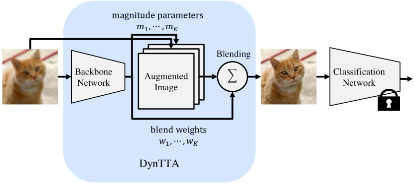
To remove this limitation and further improve the robustness while maintaining clean accuracy, we propose a novel image enhancement method, which we call DynTTA. DynTTA uses differentiable data augmentation techniques [32, 6, 21] and image blending to dynamically generate the recognition-friendly image for an input image from a huge augmentation space. Image transformation using deep neural networks are incorporated into DynTTA by considering it as a kind of data augmentation. An overview diagram of DynTTA is shown in Figure 1. DynTTA takes an image as input and outputs the magnitude parameters and blend weights for predefined data augmentation. Each augmentation is performed based on the magnitude parameters. These augmented images are linearly combined with blend weights to generate the output image. The classification model takes DynTTA’s output images as input and performs inference. Because DynTTA is composed of differentiable functions, it is directly trained with the task loss function of the recognition model. As a result, DynTTA transforms distorted images to improve recognition accuracy. In addition, we introduce a practical training and evaluation scenario, the blind setting, which does not assume the type of test-time distribution shifts and was not conducted in existing studies.
DynTTA is evaluated on two datasets and a variety of classification models, including state-of-the-art classification models such as Vision Transformer [44] and MLP-Mixer [43]. DynTTA improves the accuracy for distorted images while maintaining the accuracy for clean images, which is a better result than existing methods.
We further show that DynTTA enables us to estimate effective training-time data augmentations for distribution shifts. DynTTA weights effective test-time augmentations for distribution shifts. By using the inverse operations of the highly weighted data augmentations during training, we make classification models robust for distribution shifts.
The main contributions of this paper are as follows.
-
•
We propose DynTTA, a novel image enhancement method based on differentiable data augmentation techniques and image blending. Using it before the pretrained classification model improves robustness.
-
•
We show that DynTTA improves robustness compared to existing methods with almost no reduction in clean accuracy.
-
•
We use DynTTA to estimate the effective data augmentation during training for distribution shift, and show that retraining the classification model with the estimated data augmentations significantly improve robustness.
2 Related Work
2.1 Robustness of Deep Neural Networks
Deep neural networks are known to be vulnerable to image distortions, which often occur in the real world. These image distortions have been studied in several works. [3] showed that defects such as noise and blur in real-world sensors cause performance degradation in image recognition networks. [28] investigated that haze reduces the accuracy of image classification and experimented that the dehaze method for human visibility is not effective in improving image classification performance. [29] empirically studied real-world image degradation problems for nine kinds of degraded images—hazy, motion-blurred, fish-eye, underwater, low resolution, salt-and-peppered, white Gaussian noise, Gaussian-blurred, and out-of-focus.
Various datasets have been proposed to evaluate the robustness of deep neural networks. [5] made a style-transformed dataset to demonstrate that deep neural networks recognize objects by their texture rather than their shape. [9] proposed 19 algorithmically generated corruption datasets in five levels, belonging to four categories: noise, blur, weather, and digital. They showed that deep neural networks trained on a clean dataset decrease accuracy on these corruption datasets. In addition, they introduced the dataset of naturally occurring adversarial examples in the real world [11], and the dataset containing distribution shifts that occur in the real world, such as image style, image blurriness, geographic location, camera operation, and more [8]. In this paper, we evaluate our method on these datasets.
2.2 Training Robust Classification Models
Many works have been studied to improve the robustness of deep neural networks to naturally occurring image distortions. One way to improve the robustness is the data augmentation. [10, 47, 4] proposed a method to improve robustness by using a mix of multiple data augmentations. [34, 45] showed that adding noise during training improves the robustness to noise and other types of distortions. [24] investigated that the similarity between data augmentation and test-time image corruption is strongly correlated with the performance.
Training algorithms to improve robustness have also been studied. [49] proposed Advprop, a method to improve adversarial training, which improves not only robustness but also clean accuracy. [22] proposed an algorithm to train model by paying complementary attention to the shape and texture of objects. Since these methods are used when training recognition models, they can be used in combination with image enhancement methods, which assume that the recognition models are pretrained. Our experiments show that combining the recognition models pretrained by these methods with image enhancement methods further improves the robustness.
2.3 Image Enhancement
2.3.1 Test-time Augmentation
It is possible to improve recognition accuracy by using data augmentation not only during training-time but also during test-time. Various test-time augmentation methods have been proposed, using simple geometric transformations such as flip and crop [30, 50, 2, 18, 40, 7], mixup [19, 27], and augmentation in the embedding space [1]. [36, 16] experimentally analyzed why and when test-time augmentation works, and gave theoretical guarantees. These studies use only specific data augmentations for all test set images. Dynamically selecting the best data augmentation for each input image is expected to improve the accuracy. [25] proposed a greedy search-based test-time augmentation method to find the augmentation policy on the test set, but it is not optimal for each input image. [15] proposed a module called Loss Predictor to predict the classification loss of augmented images, allowing dynamic selection of the best one for the input image from the 12 data augmentations. However, despite the fact that the augmentation space is actually infinite, these methods have significant limitations on the augmentation space due to computational cost and the improvement in robustness is small. Our method eliminates this limitation and achieves a better robustness than existing methods by generating the best augmented image from a large augmentation space. In addition, we propose the training-time augmentation estimation method for distribution-shifted datasets using test-time augmentation, and we show that retraining the classification model by estimated augmentations significantly improves robustness.
2.3.2 Image Transformation
Several studies have been conducted to improve the recognition accuracy by image transformation using deep neural networks. [37] proposed convolutional neural network-based enhancement filters that enhance image-specific details to improve recognition accuracy. [23, 26, 39, 20] used a deep neural network model to transform degraded images into recognition-friendly images. [41] showed that not only image enhancement but also resizing at the same time improves the recognition accuracy. These methods use deep neural networks to transform images, but tend to perform excessive transformations to remove distortions, which reduces the accuracy of clean images. By considering these image enhancement methods as a kind of data augmentation, we treat them as part of DynTTA. DynTTA combines this nonlinear transformation with linear transformations of the data augmentation to improve robustness while maintaining clean accuracy.
3 DynTTA
3.1 Key Ideas
Many data augmentations have continuous magnitude parameters (e.g., rotation has a continuous magnitude parameter from 0 to 360 degrees). In addition, there are a large number of combinations of two or more data augmentations (e.g., augmentation is performed in the order of rotation, contrast, and sharpness). These facts make the augmentation space infinite. To select the best combination of data augmentations and their magnitude parameters for the test image from this infinite space, we introduce two key ideas. The first is to find the local optimal magnitude parameter by optimization. Since most data augmentations are differentiable with respect to the magnitude parameter, the local optimal magnitude parameter is obtained by optimization algorithms, such as gradient descent. This idea is inspired by recent differentiable data augmentation techniques [32, 6, 21, 33]. The second is to represent the combination of augmentation with image blending, which is the process of affine combination of multiple images. For example, if the weights are , only the 1st augmented image is selected, and if the weights are , the 1st and 3rd augmented images are combined. Note that image blending does not provide the performing order of the augmentation. We call these ideas “Blending” and “Optimization”, respectively. Based on these key ideas, we propose a novel image enhancement method, DynTTA.
3.2 Overview of DynTTA
The overview of DynTTA is shown in Figure 1. First, we define the differentiable data augmentations used in DynTTA and their range of magnitude parameters . Some data augmentations, such as rotation, have a magnitude parameter. On the other hand, other data augmentations do not have a magnitude parameter, such as auto-contrast. Details of the data augmentations used in DynTTA are shown in Section 3.3.
Any neural network can be used as the backbone of DynTTA by modifying its output layer. DynTTA takes an image as input and outputs the magnitude parameters and blend weights . is the number of data augmentations. The magnitude parameter is mapped to a value in the range or using an activation function such as sigmoid function or hyperbolic tangent function. It is then multiplied by the predefined magnitude range . The blend weights are converted to weights that sum to 1 by the softmax function. We show and in the following equation.
| (3) | ||||
| (4) |
Using the magnitude parameters and blend weights, DynTTA generates a recognition-friendly image. data augmentations are performed with magnitude parameters , then DynTTA generates a blended image by linearly combining these augmented images with . The output of DynTTA is obtained by the following equation.
| (5) | ||||
| (6) |
Where is the input image, is the k-th augmentation operation, is the k-th augmented image, and is the output image.
3.3 Augmentation Space
The data augmentations and their and used by DynTTA are shown in Table 1. We use only differentiable data augmentations.
Placing low-pass and high-pass filters within the deep neural network architecture [52, 31, 46, 12] or using them as training-time augmentation [13, 51, 38] improve robustness. Inspired by these studies, we try to improve the robustness by using low-pass and high-pass filters as test-time augmentation. These filters have a filter size parameter which is not obtained via gradient descent. Therefore, we discretize this parameter and prepare multiple filters. In this paper, we make 19 low-pass and 19 high-pass filters, each with a filter size from to in increments.
URIE uses a deep neural network to generate recognition-friendly images. Such an image transformation model is applied to DynTTA by considering it as a kind of augmentation. In this case, the image transformation model is trained simultaneously with DynTTA.
DynTTA handles many data augmentations, but is also computationally expensive. By not executing data augmentation with small blend weights, the number of data augmentation executions are significantly reduced while maintaining accuracy. We describe the details in the Appendix.
| Augmentation | ||
| Rotate | 30 | |
| Scale | 0.3 | |
| Saturate | 5.0 | |
| Contrast | 3.0 | |
| Sharpness | 10 | |
| Brightness | 0.6 | |
| A-Contrast | - | - |
| Hue | 2.0 | |
| Equalize | - | - |
| Invert | - | - |
| Gamma | 3.0 | |
| LPFs() | - | - |
| HPFs() | - | - |
| URIE | - | - |
3.4 Loss Function
DynTTA is trained by using it before inference of a pretrained classification model. When training DynTTA, the classification model is frozen. The output image of DynTTA is used as input to the classification model to calculate the cross entropy loss. Because DynTTA is differentiable, it minimizes this loss and outputs recognition-friendly images.
4 Experiments
In this section, we describe the experimental setup, experimental results comparing DynTTA to other image enhancement methods, and detailed experiments with DynTTA. We also show that robustness is significantly improved by using DynTTA to estimate the most effective training-time data augmentation for distribution shift, which is then used for retraining the classification model. Some detailed experiments are described in the Appendix.
4.1 Training and Evaluation Settings
In this paper, we use two settings, blind and non-blind settings, for training and evaluation. In the non-blind setting adopted by existing studies [15, 39] uses the corruption dataset [9]. This dataset consists of 19 types of corruption with five severity levels generated by the algorithm. 15 corruptions are used for training as Seen corruptions111Gaussian noise, Shot noise, Impulse noise, Defocus blur, Glass blur, Motion blur, Zoom blur, Snow, Frost, Fog, Brightness, Contrast, Elastic transform, Pixelate, JPEG., and four corruptions are used for testing as Unseen corruptions222Speckle noise, Gaussian blur, Spatter, Saturation.. Seen and Unseen corruptions consist of the same four categories: noise, blur, weather, and digital, so this is a setting in which we know in advance the type of corruption that occurs during the test time. In this setting, we know in advance the type of corruption (e.g. noise) in the test set, so we use this knowledge to generate artificial corruption (e.g. Gaussian noise), which we then use as Seen for training. However, this setting is often impractical because test set corruption is often unknown. Therefore, we introduce a new training and evaluation setting, the blind setting, which has no assumption on test-time distribution shifts. In the blind setting, we cannot use artificial corruptions for training, so we use data augmentations like AugMix [10] that improve the robustness to unknown corruptions. The corruption datasets are used for testing only.
4.2 Experimental Setup
We evaluate our method on two image recognition datasets, CUB [48] and ImageNet [35]. In experiments on CUB, we run all experiments three times and report the average results. We use Loss Predictor [15]() and URIE [39] as comparison methods. Classification models are prepared in advance and the backbone network of DynTTA and Loss Predictor is prepared by fine-tuning a ResNet18 [7] pretrained on ImageNet. For training in the non-blind setting, corruption is randomly selected for each mini-batch to train enhancement models. The corruptions consist of 15 Seen corruptions in five levels and clean (no corruption). For testing, we used four Unseen corruptions. In the blind setting, the enhancement models are trained using AugMix for CUB and AugMix+DeepAugment [8] for ImageNet. For testing, we used all 19 corruptions. When evaluating on the corruptions dataset, we use the average accuracy as evaluation metric. In addition to evaluating the robustness of these distribution shift datasets, we also evaluate our results on the standard clean dataset. The baseline does not use the enhancement model and the difference from the baseline is reported in the results. In the table of experiments, the best result is shown in bold, and the second best result is shown in underline.
4.3 Performance Evaluation
4.3.1 Classification on CUB
CUB is an image dataset of 200 class bird species. It consists of 5994 training images and 5794 test images. We used ResNet50 [7], Mixer-B16 [43] and DeiT-base [44] as the classification model. For optimization, we employ Adam [17] with learning rate for URIE, for DynTTA and Loss Predictor, and decay the learning rate every 10 epochs by 2. These models are trained in epochs.
We show the results in Table 2. In the non-blind setting, URIE improves Unseen accuracy but reduces the clean accuracy by a maximum of about 3.3 points. Loss Predictor does not decrease the clean accuracy, but the improvement in Unseen accuracy is small. DynTTA outperforms the comparison method in both clean accuracy and Unseen accuracy. DynTTA greatly improves the Unseen accuracy with almost no decrease in clean accuracy. Our experiments show that image enhancement methods are effective for state-of-the-art classification models such as DeiT and MLP-Mixer. It is also possible to further increase the robustness of classification models trained by AugMix. In the blind setting, similar to the non-blind setting, URIE tends to reduce the clean accuracy by a maximum of about 1.0 points. Loss Predictor improves both clean accuracy and robustness a little. DynTTA has less degradation in clean accuracy than URIE, and it is also more robust. In particular, DynTTA significantly improves the robustness of Mixer-B16 compared to existing methods. Our experiments show that AugMix-trained enhancement models slightly improve the robustness of AugMix-trained classification models.
| Non-blind | |||
| Classification | Enhancement | ||
| model | model | Clean | Unseen |
| ResNet50 | URIE | 78.39(-3.32) | 55.93(7.53) |
| LossPredictor | 81.70(-0.01) | 50.88(2.48) | |
| DynTTA | 81.58(-0.13) | 58.02(9.62) | |
| ResNet50 | URIE | 80.99(-1.56) | 63.95(3.95) |
| w/AugMix | LossPredictor | 82.59(0.04) | 60.79(0.79) |
| DynTTA | 82.64(0.09) | 65.49(5.49) | |
| Mixer-B16 | URIE | 86.73(-0.69) | 72.77(3.93) |
| LossPredictor | 87.39(-0.03) | 70.06(1.22) | |
| DynTTA | 87.56(0.14) | 73.89(5.05) | |
| Mixer-B16 | URIE | 86.61(-0.47) | 75.88(2.68) |
| w/AugMix | LossPredictor | 86.93(0.05) | 74.20(1.00) |
| DynTTA | 87.26(0.38) | 76.58(3.38) | |
| DeiT-base | URIE | 83.91(-1.25) | 68.61(1.79) |
| LossPredictor | 85.16(0.00) | 67.47(0.65) | |
| DynTTA | 84.79(-0.37) | 69.80(2.98) | |
| DeiT-base | URIE | 83.88(-0.29) | 70.56(1.50) |
| w/AugMix | LossPredictor | 84.20(0.03) | 69.64(0.58) |
| DynTTA | 84.42(0.25) | 71.76(2.70) | |
| Blind | |||
| Classification | Enhancement | ||
| model | model | Clean | Corruption |
| ResNet50 | URIE | 80.68(-1.03) | 51.47(2.89) |
| LossPredictor | 81.75(0.04) | 48.61(0.03) | |
| DynTTA | 81.65(-0.06) | 51.97(3.39) | |
| ResNet50 | URIE | 82.75(0.20) | 62.05(0.30) |
| w/AugMix | LossPredictor | 82.65(0.10) | 61.76(0.01) |
| DynTTA | 82.84(0.29) | 62.39(0.64) | |
| Mixer-B16 | URIE | 87.04(-0.38) | 71.27(0.07) |
| LossPredictor | 87.49(0.07) | 71.78(0.58) | |
| DynTTA | 87.37(-0.05) | 72.74(1.54) | |
| Mixer-B16 | URIE | 86.89(0.01) | 74.41(0.04) |
| w/AugMix | LossPredictor | 86.95(0.07) | 74.44(0.07) |
| DynTTA | 87.12(0.24) | 75.46(1.09) | |
| DeiT-base | URIE | 84.71(-0.45) | 67.44(0.96) |
| LossPredictor | 85.21(0.05) | 66.49(0.01) | |
| DynTTA | 85.06(-0.10) | 67.37(0.89) | |
| DeiT-base | URIE | 84.21(0.04) | 70.38(0.10) |
| w/AugMix | LossPredictor | 84.21(0.04) | 70.28(0.00) |
| DynTTA | 84.31(0.14) | 70.35(0.07) |
4.3.2 Classification on ImageNet
ImageNet is the most widely used 1000-class image recognition dataset. It is composed of 1.3 million training images and 50,000 test images. We used ResNet50 and DeiT as the classification model. For optimization, we employ Adam with learning rate for URIE, for DynTTA and Loss Predictor, and decay the learning rate every 8 epochs by 10. These models are trained in epochs.
We show the results in Table 3. In the non-blind setting, URIE improves Unseen accuracy but reduces the clean accuracy by a maximum of about 1.6 points. Loss Predictor does not decrease the ResNet50 clean accuracy, but the improvement in Unseen accuracy is small. In DeiT, Loss Predictor showed a decrease in both clean and Unseen accuracy. DynTTA slightly reduces the clean accuracy, but the improvement in Unseen accuracy is higher than the comparison method. In the blind setting, URIE and Loss Predictor experiments showed almost the same trend results as in the non-blind setting. DynTTA improves robustness over URIE without degrading the clean accuracy.
| Non-blind | |||
| Classification | Enhancement | ||
| model | model | Clean | Unseen |
| ResNet50 | URIE | 74.56(-1.57) | 49.05(3.96) |
| LossPredictor | 76.12(-0.01) | 46.03(0.94) | |
| DynTTA | 75.89(-0.24) | 50.55(5.46) | |
| DeiT-base | URIE | 81.01(-0.73) | 67.50(2.19) |
| LossPredictor | 81.09(-0.65) | 64.22(-1.09) | |
| DynTTA | 81.25(-0.50) | 67.92(2.61) | |
| Blind | |||
| Classification | Enhancement | ||
| model | model | Clean | Corruption |
| ResNet50 | URIE | 74.71(-1.42) | 44.19(4.62) |
| LossPredictor | 76.13(0.00) | 40.29(0.72) | |
| DynTTA | 76.04(-0.09) | 44.87(5.30) | |
| DeiT-base | URIE | 80.69(-1.06) | 62.69(1.07) |
| LossPredictor | 80.76(-0.98) | 60.28(-1.34) | |
| DynTTA | 81.75(0.01) | 62.71(1.08) |
4.4 Ablation Study
4.4.1 Effects of Key Ideas
We conduct an ablation study of our key ideas by using ResNet50 on the CUB dataset and comparing it to Loss Predictor. Loss Predictor selects one best augmentation for a test image by learning the classification losses of 12 augmented images333Identity; {-20, 20} Rotate; {0.8, 1.2} Zoom; {0.5, 2.0} Saturate; Auto-contrast; {0.2, 0.5, 2.0, 4.0} Sharpness as a label. One of our key ideas, “Blending”, improves upon Loss Predictor by using not just one image but a combination of many augmented images. Image blending is lightweight because it does not require the computation of classification losses, which has the advantage of being easily extendable in augmentation space by adding data augmentations. Here we define DynTTA(Blending), which has the same augmentation and magnitude parameters as Loss Predictor and outputs only blend weights. We measure the effect of the “Blending” by using DynTTA(Blending). In addition, to measure the effect of “Optimization”, we define DynTTA(BlendingOptimization) that extends the DynTTA(Blending) and simultaneously outputs magnitude parameters. At this time, we set the magnitude parameter ranges the same as in Table 1 except for Zoom, and Identity is not used because it is included in some data augmentations (e.g., a rotation of 0 degrees).
The results are shown in Table 4. DynTTA(Blending) is much more robust than the Loss Predictor. This result means that multiple-image blending is better than choosing one best image. In the non-blind setting, DynTTA(BlendingOptimization) shows a worse Unseen accuracy than DynTTA(Blending). This is because the magnitude parameters used by the Loss Predictor and “Blending” may have been tuned by the authors for their non-blind setting experiment. On the other hand, in the blind setting, DynTTA(BlendingOptimization) achieved better robustness than DynTTA(Blending). This is because “Optimization” automatically find the local optimal magnitude parameters for the blind setting using gradient descent.
| Non-blind | |||
|---|---|---|---|
| Enhancement model | Clean | Unseen | |
| DynTTA(Blending) | 81.64(-0.06) | 52.49(1.61) | |
| DynTTA(BlendingOptimization) | 81.68(-0.02) | 52.15(1.27) | |
| Blind | |||
| Enhancement model | Clean | Corruption | |
| DynTTA(Blending) | 81.71(-0.04) | 51.12(2.51) | |
| DynTTA(BlendingOptimization) | 81.73(-0.02) | 51.51(2.90) |
4.4.2 Effects of Augmentation Space
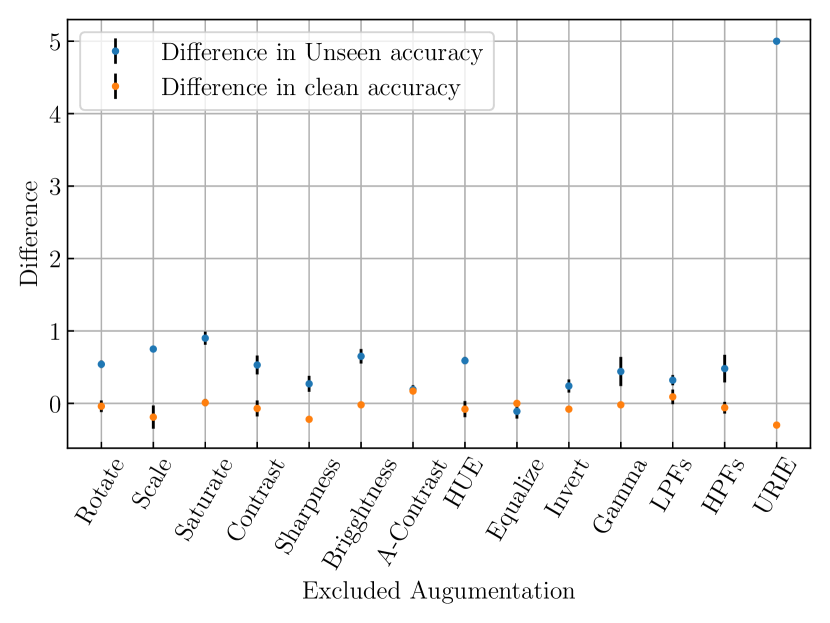
In this paper, the 14 data augmentations shown in Table 1 are used for DynTTA. We investigate the contribution of each data augmentation to classification accuracy in the non-blind setting using ResNet50 on the CUB dataset. Figure 2 shows the accuracy when each augmentation is excluded from DynTTA before training. All data augmentations, except Equalize contribute to improving robustness with almost no reduction in clean accuracy. In particular, the contribution of URIE to improving robustness is very significant, but URIE tends to degrade clean accuracy. DynTTA blends URIE with other data augmentations to maintain the clean accuracy.
4.5 Detailed Experiments
In this section, we experiment on the CUB dataset using ResNet50 as the classification model to understand the details of DynTTA.
4.5.1 Effects of Magnitude Range
We investigate the effect of different magnitude ranges on classification accuracy. In the experiments in the blind setting here, we also experimented with the stylized dataset [5] in addition to the corruption dataset. The range in Table 1 multiplied by is referred to “Large”, and the range multiplied by is referred to “Small”.
The results are shown in the Table 5. “Small” showed a better result for corruption dataset and “Large” for stylized dataset. The clean accuracy of “Large” is a little lower than the others. We observed that a large magnitude range is effective for large distribution shifts such as stylized datasets, but large image transformations degrade clean accuracy. “Small” showed more robust than the standard range. This may be caused by the fact that “Small” has a smaller search space and the optimization is more stable.
| Non-blind | |||
|---|---|---|---|
| Range | Clean | Unseen | |
| Small | 81.58(0.00) | 58.41(0.39) | |
| Large | 81.26(-0.32) | 57.80(-0.22) | |
| Blind | |||
| Range | Clean | Corruption | Stylized |
| Small | 81.65(0.00) | 52.62(0.65) | 18.35(0.19) |
| Large | 81.61(-0.04) | 52.32(0.35) | 18.50(0.34) |
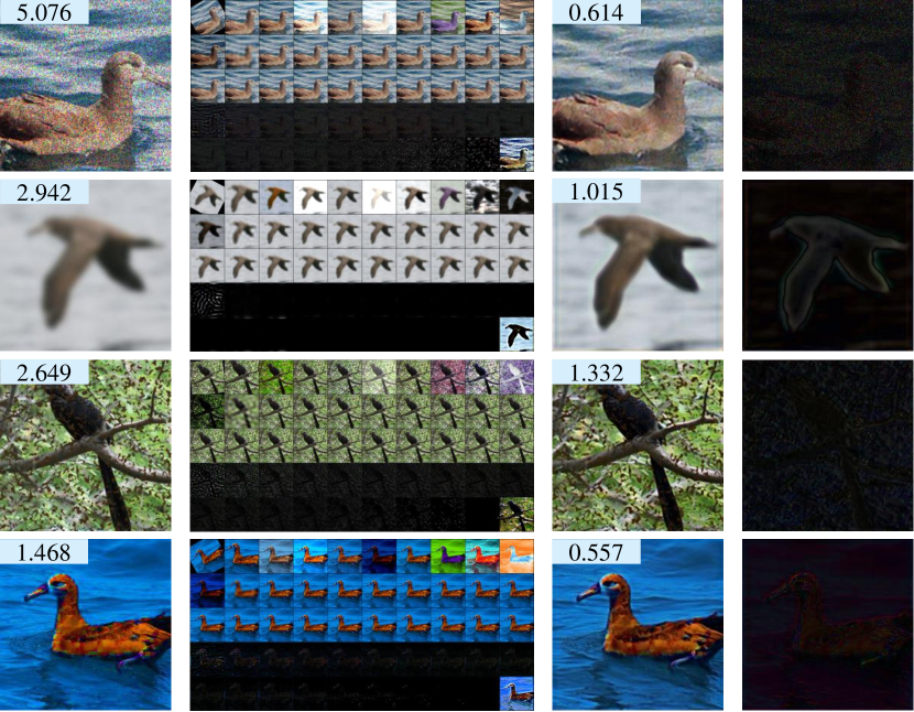
4.5.2 Visualization of DynTTA Output
We visualize the output of DynTTA in the non-blind setting. We show augmented images and output image by DynTTA for level five Unseen corruptions in Figure 3. The bottom two rows of augmented images are almost black, except for the bottom right, so hard for us to see what they show, but this is because high-pass filters remove low-frequency domains that are visible to humans. Speckle Noise image is denoised and Gaussian Blur image is sharpened. The corruption in Spatter and Saturate images have not been removed, but the shape and texture of the object are enhanced.
4.6 Estimation of Training Time Augmentation for Distribution-Shifted Datasets
In this section we describe a different use of DynTTA, estimating training time augmentation for distribution-shifted datasets. For distribution-shifted test dataset, DynTTA weights effective test-time augmentations that improve accuracy. The distribution shift is expected to consist of inverse operations of the highly weighted data augmentations. For example, the distribution-shifted test dataset, where low-pass filters are effective, is expected to contain more high-frequency content than the training dataset. Using a high-pass filter on the training dataset during retraining allows the classification model to recognize based on high-frequency components, and it is expected to improve the accuracy on the distribution-shifted test dataset. Therefore, we consider that retraining the recognition model using inverse operations of highly weighted data augmentations improve the accuracy for the distribution-shifted datasets.
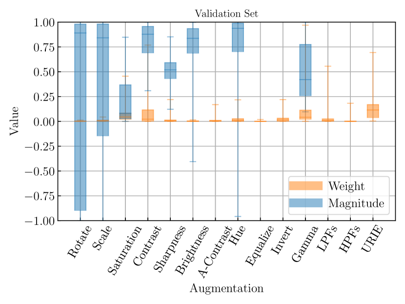
In the blind setting, we split the level five Unseen corruption test set into a validation set and a test set in a 2:8 ratio. Figure 4 shows a visualization of the magnitude parameters and the blend weights, which are the outputs of DynTTA for the validation set. DynTTA outputs high blend weights of low-pass filters, which are effective for high-frequency corruptions such as Speckle Noise and Spatter, and of saturation, which is effective for Saturate. The maximum weights of low-pass filters, gamma, contrast, and saturation are high for validation set. The magnitude parameters of rotate and scale have high variance. This is because when the blend weight is close to zero, any value of the magnitude parameter has almost no effect on the output image.
Next, from the test-time augmentation that was effective for the validation set, we estimate the training-time augmentation that is effective for the target corruption. Based on the results in Figure 4, we focus on the maximum value of the blend weights rather than the magnitude parameter. We choose the four data augmentations used to retrain the classification model: high-pass filters, gamma, contrast, and saturation, which are the inverse operations of four data augmentations that were effective for validation set. We experiment by varying the data augmentation space used by the AugMix. The results of the Unseen test set are shown in Table 6. “Normal” is the normal AugMix and uses nine data augmentations 444Auto-Contrast, Equalize, Posterize, Rotate, Solarize, ShearX, ShearY, TranslateX, TranslateY. “All” is the normal nine data augmentations plus saturation, contrast, brightness and sharpness, referenced from the official AugMix implementation and “Estimated” is the normal nine data augmentations plus saturation, contrast, high-pass filters and gamma. The classification model trained with “Estimated” achieved the best accuracy for all corruptions except Saturate. On average, it was approximately 10 points more accurate than “Normal”, and, in particular, approximately 20 points more accurate than “Normal” for Speckle Noise.
| Corruption | Normal | All | Estimated |
|---|---|---|---|
| Speckle Noise | 50.27 | 49.90 | 70.25 |
| Gaussian Blur | 30.49 | 33.18 | 37.22 |
| Spatter | 35.33 | 35.61 | 43.36 |
| Saturate | 36.75 | 44.97 | 42.74 |
| Average | 38.21 | 40.92 | 48.39 |
5 Conclusions
In this paper, we propose DynTTA, a novel image enhancement method based on differentiable data augmentation techniques and image blending. DynTTA uses a gradient descent algorithm to find magnitude parameters and blend weights from a huge augmentation space. This augmentation space includes deep neural networks such as URIE as well as standard data augmentation. DynTTA improves robustness by using it before inference of the classification model without retraining the classification model. Existing image enhancement studies are evaluated under the assumption that they know the type of test-time distribution shifts. We introduce a practical training and evaluation scenario that does not assume the type of test-time distribution shifts. Our experiments, which included state-of-the-art classification models, showed that DynTTA outperforms existing methods and improves robustness with almost no reduction in clean accuracy. We showed that image enhancement methods further improve the robustness of such robust classification models trained by AugMix and modern classification models such as ViT and MLP-Mixer are highly robust. Furthermore, DynTTA estimated effective learning time augmentation for the distribution-shifted datasets and showed that retraining with such augmentation greatly improves robustness.
In this paper, we experimented only with the image classification task. We will apply and evaluate DynTTA to other tasks such as object detection and segmentation. The search for the best architecture for DynTTA and the reduction of computational cost are also future works.
References
- [1] Arsenii Ashukha, Andrei Atanov, and Dmitry Vetrov. Mean embeddings with test-time data augmentation for ensembling of representations. arXiv preprint arXiv:2106.08038, 2021.
- [2] Christian Clausner, Apostolos Antonacopoulos, and Stefan Pletschacher. Icdar2019 competition on recognition of documents with complex layouts - rdcl2019. In International Conference on Document Analysis and Recognition (ICDAR), 2019.
- [3] Steven Diamond, Vincent Sitzmann, Frank Julca-Aguilar, Stephen Boyd, Gordon Wetzstein, and Felix Heide. Dirty pixels: Towards end-to-end image processing and perception. ACM Transactions on Graphics (TOG), 2021.
- [4] N Benjamin Erichson, Soon Hoe Lim, Francisco Utrera, Winnie Xu, Ziang Cao, and Michael W Mahoney. Noisymix: Boosting robustness by combining data augmentations, stability training, and noise injections. arXiv preprint arXiv:2202.01263, 2022.
- [5] Robert Geirhos, Patricia Rubisch, Claudio Michaelis, Matthias Bethge, Felix A Wichmann, and Wieland Brendel. Imagenet-trained CNNs are biased towards texture; increasing shape bias improves accuracy and robustness. In International Conference on Learning Representations (ICLR), 2019.
- [6] Ryuichiro Hataya, Jan Zdenek, Kazuki Yoshizoe, and Hideki Nakayama. Faster AutoAugment: Learning Augmentation Strategies using Backpropagation. In European Conference on Computer Vision (ECCV), 2020.
- [7] Kaiming He, Xiangyu Zhang, Shaoqing Ren, and Jian Sun. Deep residual learning for image recognition. In IEEE/CVF Conference on Computer Vision and Pattern Recognition (CVPR), 2016.
- [8] Dan Hendrycks, Steven Basart, Norman Mu, Saurav Kadavath, Frank Wang, Evan Dorundo, Rahul Desai, Tyler Zhu, Samyak Parajuli, Mike Guo, et al. The many faces of robustness: A critical analysis of out-of-distribution generalization. In IEEE/CVF International Conference on Computer Vision (ICCV), 2021.
- [9] Dan Hendrycks and Thomas Dietterich. Benchmarking neural network robustness to common corruptions and perturbations. In International Conference on Learning Representations (ICLR), 2019.
- [10] Dan Hendrycks, Norman Mu, Ekin D. Cubuk, Barret Zoph, Justin Gilmer, and Balaji Lakshminarayanan. AugMix: A simple data processing method to improve robustness and uncertainty. In International Conference on Learning Representations (ICLR), 2020.
- [11] Dan Hendrycks, Kevin Zhao, Steven Basart, Jacob Steinhardt, and Dawn Song. Natural adversarial examples. In IEEE/CVF Conference on Computer Vision and Pattern Recognition (CVPR), 2021.
- [12] Md Tahmid Hossain, Shyh Wei Teng, Ferdous Sohel, and Guojun Lu. Robust image classification using a low-pass activation function and dct augmentation. IEEE Access, 2021.
- [13] Md Tahmid Hossain, Shyh Wei Teng, Dengsheng Zhang, Suryani Lim, and Guojun Lu. Distortion robust image classification using deep convolutional neural network with discrete cosine transform. In IEEE International Conference on Image Processing (ICIP), 2019.
- [14] Andrew Howard, Mark Sandler, Grace Chu, Liang-Chieh Chen, Bo Chen, Mingxing Tan, Weijun Wang, Yukun Zhu, Ruoming Pang, Vijay Vasudevan, et al. Searching for mobilenetv3. In IEEE/CVF International Conference on Computer Vision (ICCV), 2019.
- [15] Ildoo Kim, Younghoon Kim, and Sungwoong Kim. Learning loss for test-time augmentation. In Advances in Neural Information Processing Systems (NeurIPS), 2020.
- [16] Masanari Kimura. Understanding test-time augmentation. In Neural Information Processing, 2021.
- [17] Diederik P Kingma and Jimmy Ba. Adam: A method for stochastic optimization. In International Conference on Learning Representations (ICLR), 2015.
- [18] Alex Krizhevsky, Ilya Sutskever, and Geoffrey E Hinton. Imagenet classification with deep convolutional neural networks. In Advances in neural information processing systems (NeurIPS), 2012.
- [19] Hansang Lee, Haeil Lee, Helen Hong, and Junmo Kim. Test-time mixup augmentation for uncertainty estimation in skin lesion diagnosis. In Medical Imaging with Deep Learning (MIDL), 2021.
- [20] Younkwan Lee, Jihyo Jeon, Yeongmin Ko, Byunggwan Jeon, and Moongu Jeon. Task-driven deep image enhancement network for autonomous driving in bad weather. In IEEE International Conference on Robotics and Automation (ICRA), 2021.
- [21] Yonggang Li, Guosheng Hu, Yongtao Wang, Timothy M. Hospedales, Neil Martin Robertson, and Yongxin Yang. DADA: differentiable automatic data augmentation. In European Conference on Computer Vision (ECCV), 2020.
- [22] Yingwei Li, Qihang Yu, Mingxing Tan, Jieru Mei, Peng Tang, Wei Shen, Alan Yuille, et al. Shape-texture debiased neural network training. In International Conference on Learning Representations (ICLR), 2020.
- [23] Ding Liu, Bihan Wen, Xianming Liu, Zhangyang Wang, and Thomas S. Huang. When image denoising meets high-level vision tasks: A deep learning approach. In International Joint Conference on Artificial Intelligence (IJCAI), 2018.
- [24] Eric Mintun, Alexander Kirillov, and Saining Xie. On interaction between augmentations and corruptions in natural corruption robustness. In Advances in Neural Information Processing Systems (NeurIPS), 2021.
- [25] Dmitry Molchanov, Alexander Lyzhov, Yuliya Molchanova, Arsenii Ashukha, and Dmitry Vetrov. Greedy policy search: A simple baseline for learnable test-time augmentation. arXiv preprint arXiv:2002.09103, 2020.
- [26] Takayuki Okatani, Xing Liu, and Masanori Suganuma. Improving generalization ability of deep neural networks for visual recognition tasks. In Computational Color Imaging Workshop (CCIW), 2019.
- [27] Tianyu Pang, Kun Xu, and Jun Zhu. Mixup inference: Better exploiting mixup to defend adversarial attacks. In International Conference on Learning Representations (ICLR), 2019.
- [28] Yanting Pei, Yaping Huang, Qi Zou, Yuhang Lu, and Song Wang. Does haze removal help cnn-based image classification? In European Conference on Computer Vision (ECCV), 2018.
- [29] Yanting Pei, Yaping Huang, Qi Zou, Xingyuan Zhang, and Song Wang. Effects of image degradation and degradation removal to cnn-based image classification. IEEE Transactions on Pattern Analysis and Machine Intelligence (TPAMI), 2021.
- [30] Juan C Perez, Motasem Alfarra, Guillaume Jeanneret, Laura Rueda, Ali Thabet, Bernard Ghanem, and Pablo Arbelaez. Enhancing adversarial robustness via test-time transformation ensembling. In IEEE/CVF International Conference on Computer Vision Workshops (ICCVW), 2021.
- [31] Yongming Rao, Wenliang Zhao, Zheng Zhu, Jiwen Lu, and Jie Zhou. Global filter networks for image classification. In Advances in Neural Information Processing Systems (NeurIPS), 2021.
- [32] Edgar Riba, Dmytro Mishkin, Daniel Ponsa, Ethan Rublee, and Gary Bradski. Kornia: an open source differentiable computer vision library for pytorch. In IEEE/CVF Winter Conference on Applications of Computer Vision (WACV), 2020.
- [33] Cédric Rommel, Thomas Moreau, and Alexandre Gramfort. Deep invariant networks with differentiable augmentation layers. In Advances in Neural Information Processing Systems (NeurIPS), 2022.
- [34] Evgenia Rusak, Lukas Schott, Roland S Zimmermann, Julian Bitterwolf, Oliver Bringmann, Matthias Bethge, and Wieland Brendel. A simple way to make neural networks robust against diverse image corruptions. In European Conference on Computer Vision (ECCV), 2020.
- [35] Olga Russakovsky, Jia Deng, Hao Su, Jonathan Krause, Sanjeev Satheesh, Sean Ma, Zhiheng Huang, Andrej Karpathy, Aditya Khosla, Michael Bernstein, et al. Imagenet large scale visual recognition challenge. International journal of computer vision (IJCV), 2015.
- [36] Divya Shanmugam, Davis Blalock, Guha Balakrishnan, and John Guttag. Better aggregation in test-time augmentation. In IEEE/CVF International Conference on Computer Vision (ICCV), 2021.
- [37] Vivek Sharma, Ali Diba, Davy Neven, Michael S. Brown, Luc Van Gool, and Rainer Stiefelhagen. Classification-driven dynamic image enhancement. In IEEE/CVF Conference on Computer Vision and Pattern Recognition (CVPR), 2018.
- [38] Ryan Soklaski, Michael Yee, and Theodoros Tsiligkaridis. Fourier-based augmentations for improved robustness and uncertainty calibration. In Workshop on Distribution Shifts: Connecting Methods and Applications (DistShift), 2021.
- [39] Taeyoung Son, Juwon Kang, Namyup Kim, Sunghyun Cho, and Suha Kwak. Urie: Universal image enhancement for visual recognition in the wild. In European Conference on Computer Vision (ECCV), 2020.
- [40] Christian Szegedy, Wei Liu, Yangqing Jia, Pierre Sermanet, Scott Reed, Dragomir Anguelov, Dumitru Erhan, Vincent Vanhoucke, and Andrew Rabinovich. Going deeper with convolutions. In IEEE/CVF Conference on Computer Vision and Pattern Recognition (CVPR), 2015.
- [41] Hossein Talebi and Peyman Milanfar. Learning to resize images for computer vision tasks. In IEEE/CVF International Conference on Computer Vision (CVPR), 2021.
- [42] Mingxing Tan and Quoc Le. Efficientnet: Rethinking model scaling for convolutional neural networks. In International Conference on Machine Learning (ICML), 2019.
- [43] Ilya O Tolstikhin, Neil Houlsby, Alexander Kolesnikov, Lucas Beyer, Xiaohua Zhai, Thomas Unterthiner, Jessica Yung, Andreas Steiner, Daniel Keysers, Jakob Uszkoreit, et al. Mlp-mixer: An all-mlp architecture for vision. In Advances in Neural Information Processing Systems (NeurIPS), 2021.
- [44] Hugo Touvron, Matthieu Cord, Matthijs Douze, Francisco Massa, Alexandre Sablayrolles, and Herve Jegou. Training data-efficient image transformers & distillation through attention. In International Conference on Machine Learning (ICML), 2021.
- [45] Athanasios Tsiligkaridis and Theodoros Tsiligkaridis. Misclassification-aware gaussian smoothing and mixed augmentations improves robustness against domain shifts. arXiv preprint arXiv:2104.01231, 2021.
- [46] Cristina Vasconcelos, Hugo Larochelle, Vincent Dumoulin, Rob Romijnders, Nicolas Le Roux, and Ross Goroshin. Impact of aliasing on generalization in deep convolutional networks. In IEEE/CVF International Conference on Computer Vision (ICCV), 2021.
- [47] Haotao Wang, Chaowei Xiao, Jean Kossaifi, Zhiding Yu, Anima Anandkumar, and Zhangyang Wang. Augmax: Adversarial composition of random augmentations for robust training. In Advances in Neural Information Processing Systems (NeurIPS), 2021.
- [48] P. Welinder, S. Branson, T. Mita, C. Wah, F. Schroff, S. Belongie, and P. Perona. Caltech-UCSD Birds 200. Technical report, California Institute of Technology, 2010.
- [49] Cihang Xie, Mingxing Tan, Boqing Gong, Jiang Wang, Alan L Yuille, and Quoc V Le. Adversarial examples improve image recognition. In IEEE/CVF Conference on Computer Vision and Pattern Recognition (CVPR), 2020.
- [50] Xulei Yang, Zeng Zeng, Sin G Teo, Li Wang, Vijay Chandrasekhar, and Steven Hoi. Deep learning for practical image recognition: Case study on kaggle competitions. In ACM SIGKDD international conference on knowledge discovery & data mining (KDD), 2018.
- [51] Dong Yin, Raphael Gontijo Lopes, Jon Shlens, Ekin Dogus Cubuk, and Justin Gilmer. A fourier perspective on model robustness in computer vision. In Advances in Neural Information Processing Systems (NeurIPS), 2019.
- [52] Xueyan Zou, Fanyi Xiao, Zhiding Yu, and Yong Jae Lee. Delving deeper into anti-aliasing in convnets. In British Machine Vision Conference (BMVC), 2020.
Appendix A Appendix
In this Supplementary Material, we provide additional analysis for the DynTTA.
A.1 Computational Cost Reduction for DynTTA
Compared with Loss Predictor, DynTTA is computationally expensive because it performs many data augmentations during inference. To reduce the inference cost of DynTTA, we tried to avoid executing data augmentations with small blend weights. With this method, we achieved a 72% reduction in the number of data augmentation executions while maintaining the accuracy of DynTTA. We describe the details here.
The method is described in the following. First, we set a threshold. If all the blend weights of a data augmentation in a mini-batch are below the threshold, we do not execute that data augmentation. Since the blend weights should add up to 1, the blend weights for the data augmentations not executed at this time are added to the blend weights of the next data augmentation that is executed. We used ResNet50 in the non-blind setting on the CUB corruption dataset at severity level 5 to measure the average number of data augmentation executions per inference and accuracy of DynTTA.
Results are shown in Table 7. When the threshold is 0, DynTTA executes all 50 data augmentations. When the threshold is less than 0.01, DynTTA reduces the average number of data augmentation executions further improving accuracy. We suspect this to be because we were able to prevent the execution of data augmentations that should not have been executed, which were output with blend weights near zero. When the threshold is 0.05, DynTTA reduces the number of data augmentation executions by about 72% while maintaining accuracy. When the threshold is greater than 0.1, DynTTA reduces the number of data augmentation executions, but it also reduces the accuracy.
| Number of | |||
|---|---|---|---|
| Threshold | Executions | Clean | Unseen |
| 0.005 | 34.76(-15.24) | 81.58(0.05) | 36.61(0.71) |
| 0.01 | 28.71(-21.29) | 81.65(0.12) | 36.68(0.78) |
| 0.02 | 21.85(-28.15) | 81.36(-0.17) | 35.81(-0.09) |
| 0.05 | 13.94(-36.06) | 81.15(-0.38) | 35.92(0.02) |
| 0.1 | 9.29(-40.71) | 80.95(-0.58) | 34.58(-1.32) |
| 0.2 | 3.88(-46.12) | 80.88(-0.65) | 19.89(-16.01) |
A.2 Detailed Experiments in section 4.3.1
Loss Predictor improves accuracy by ensembling candidate augmentations and further improves accuracy by ensembling with hflip. In Table 8 we show the accuracy of Loss Predictor () in the non-blind setting, and also in combination with hflip.
The increase in clean accuracy and robustness with is pt and pt, respectively, and was used in all main experiments due to the significantly lower robustness of Loss Predictor () compared to URIE and DynTTA. Loss Predictor also improved clean accuracy and robustness by pt and pt, respectively, when combined with hflip. However, hflip is also applicable to DynTTA, which improved by pt and pt, respectively.
| Enhancement model | Clean | Unseen |
|---|---|---|
| LP() | 82.14(0.44) | 50.97(0.09) |
| LP()hflip | 82.54(0.84) | 51.57(0.69) |
| DynTTAhflip | 82.32(0.74) | 58.72(0.70) |
A.3 Backbone Network of DynTTA
Any neural network can be used as the backbone network of DynTTA. We examine the effect of backbone network selection. We use four backbone models: ResNet18, ResNet50 [7], EfficientNet-b0 [42], and MobileNetV3 [14].
The results are shown in the Table 9. ResNet18 shows the highest robustness in the non-blind setting. EfficientNet-b0 and MobileNetV3 are more robust than ResNet in the blind setting, but the degradation of clean accuracy is higher in the non-blind setting. ResNet50 is a model with a higher classification accuracy than ResNet18, but we have found that there is no correlation between the accuracy of the model as a classification model and the performance of the model as an enhancement model.
| Non-blind | ||
| Backbone Network | Clean | Unseen |
| ResNet18 | 81.58(-0.13) | 58.02(9.62) |
| ResNet50 | 81.74(0.03) | 57.56(9.16) |
| EfficientNet-b0 | 81.27(-0.44) | 57.37(8.97) |
| MobileNetV3 | 81.08(-0.63) | 57.65(9.25) |
| Blind | ||
| Backbone Network | Clean | Corruption |
| ResNet18 | 81.65(-0.06) | 51.97(3.39) |
| ResNet50 | 81.73(0.02) | 52.07(3.49) |
| EfficientNet-b0 | 81.73(0.02) | 52.95(4.37) |
| MobileNetV3 | 81.73(0.02) | 53.00(4.42) |
A.4 Performance Evaluation Using a Classification Model Different from the One Used During Training
In this section, we discuss the generalizability of image enhancement models to classification models other than what was used for its training. Usually, there is a one-to-one correspondence between image enhancement models and classification models. We investigate whether an image enhancement model trained in couple with one classification model is also beneficial for another classification model. The results of the image enhancement models trained with ResNet50, MLoss Predictor-Mixer, and DeiT in the non-blind setting on the CUB dataset are shown in Tables 12, 12, and 12, respectively. URIE trained on ResNet50 significantly reduces clean accuracy and does not improve robustness. URIE trained with MLoss Predictor-Mixer or DeiT reduces clean accuracy by about 1-2%, but improves robustness. Loss Predictor improves robustness with almost no reduction in clean accuracy. DynTTA trained with ResNet50 has about 1% reduction in clean accuracy but improves robustness. DynTTA trained with MLoss Predictor-Mixer or DeiT improves robustness over comparison methods with almost no reduction in clean accuracy. Our experiments show that when the coupled classification model is a high accuracy model such as MLoss Predictor-Mixer or DeiT, the generalization ability of the image enhancement model is high. In particular, DynTTA improves robustness over comparison methods with almost no reduction in clean accuracy, which is a high generalization ability. DynTTA trained with a highly accurate classification model shows its potential to be applied to a variety of classification models.
| Classification | Enhancement | ||
|---|---|---|---|
| model | model | Clean | Unseen |
| Mixer-B16 | URIE | 83.76(-3.66) | 68.94(0.10) |
| LossPredictor | 87.38(-0.04) | 69.91(1.07) | |
| DynTTA | 86.55(-0.87) | 71.86(3.02) | |
| DeiT | URIE | 81.65(-3.51) | 64.45(-2.37) |
| LossPredictor | 85.13(-0.03) | 67.25(0.43) | |
| DynTTA | 84.25(-1.01) | 67.81(1.09) |
| Classification | Enhancement | ||
|---|---|---|---|
| model | model | Clean | Unseen |
| ResNet50 | URIE | 80.80(-1.01) | 52.99(4.59) |
| LossPredictor | 81.74(0.03) | 50.67(2.27) | |
| DynTTA | 82.03(0.32) | 53.29(4.89) | |
| DeiT | URIE | 84.35(-0.81) | 67.61(0.79) |
| LossPredictor | 85.13(-0.03) | 67.25(0.43) | |
| DynTTA | 85.02(-0.14) | 69.29(2.47) |
| Classification | Enhancement | ||
|---|---|---|---|
| model | model | Clean | Unseen |
| ResNet50 | URIE | 79.85(-1.86) | 51.51(3.11) |
| LossPredictor | 81.72(0.01) | 49.95(1.55) | |
| DynTTA | 81.60(-0.11) | 53.23(4.83) | |
| Mixer-B16 | URIE | 86.07(-1.35) | 71.35(2.51) |
| LossPredictor | 87.37(-0.05) | 69.55(0.71) | |
| DynTTA | 87.14(-0.28) | 72.77(3.93) |
A.5 Comparison with Test-Time Augmentation
The Loss Predictor paper made a comparison with some simple test-time augmentation (center crop, horizontal flip, random augmentation selection), and the results are that the Loss Predictor is better. Therefore, DynTTA should also be better than simple test-time augmentation. On the other hand, training time augmentation, which randomly combines (blends) multiple images to improve robustness (e.g. AugMix), has recently been proposed. Random blending of multiple images during training has the effect of improving robustness, however, it is not clear whether it has the same effect during testing. To verify the effect of randomly blending images during testing, we experimented with test-time AugMix using ResNet50 in the blind setting on the CUB dataset. The resulting clean accuracy is 67.64% and corruption accuracy is 36.12%, which is significantly worse than the baseline (without image enhancement model). This result indicates that simple randomly blending is ineffective and that blending trained by DynTTA is effective in improving robustness.
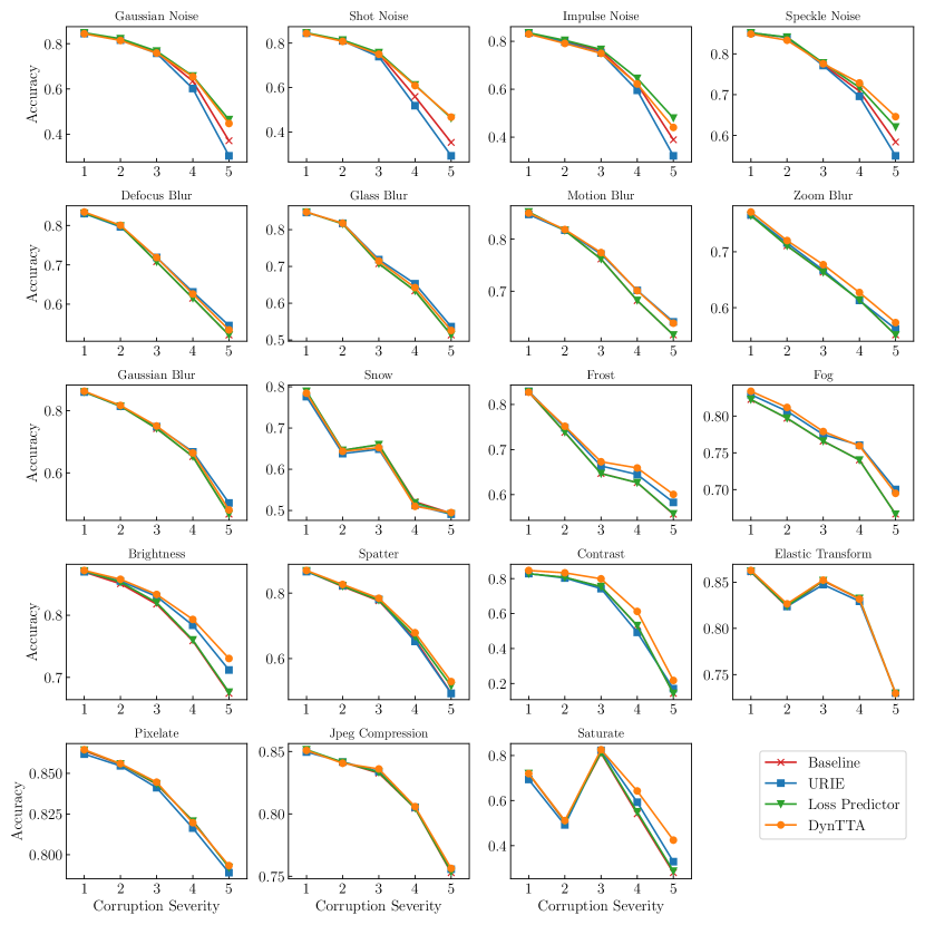
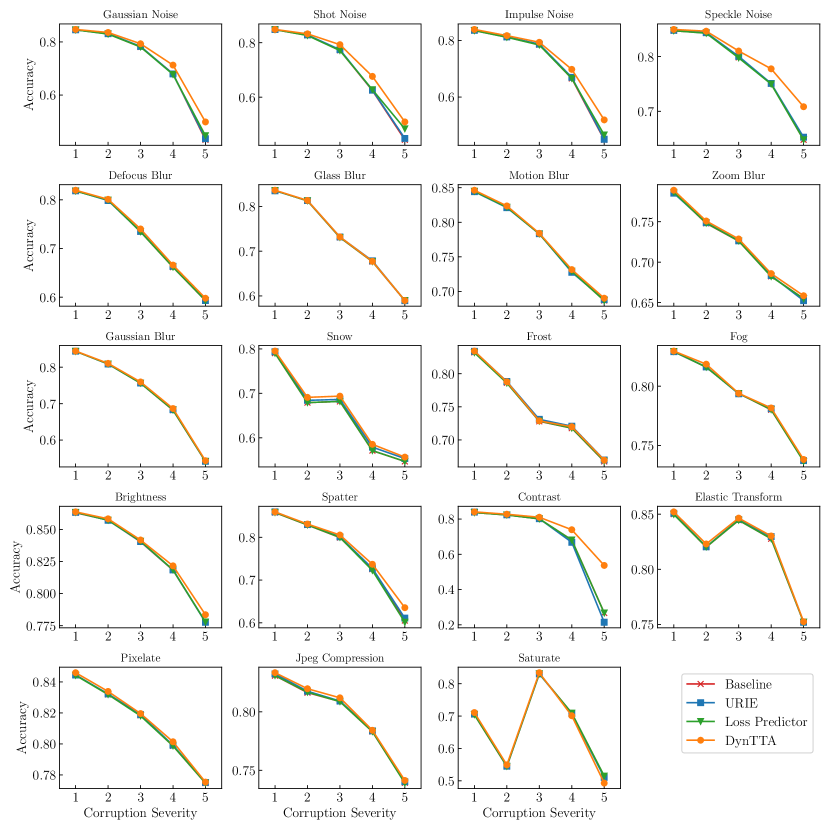
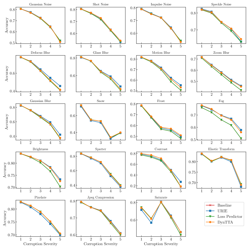
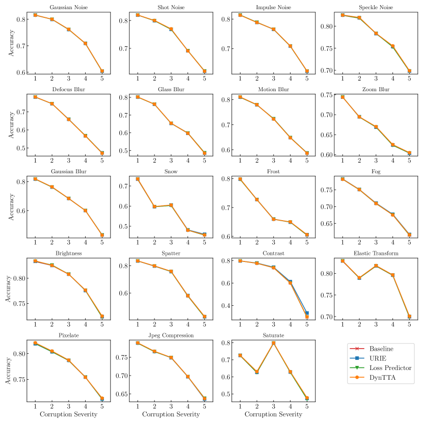
A.6 Details of the CUB Dataset Experiment
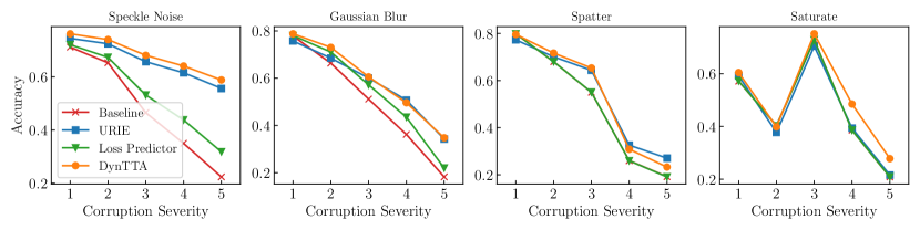
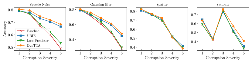
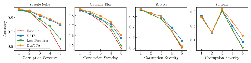
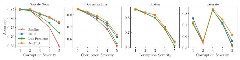
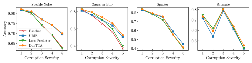
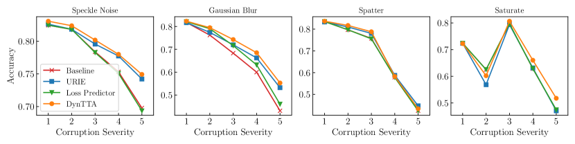
In this section, we show the accuracy for each corruption and severity results of the CUB dataset experiment presented in section 4.2. The results of the non-blind setting are shown in Figures 8-10. For Gaussian Noise and Gaussian Blur, DynTTA improves accuracy over comparison methods regardless of severity. For Spatter, DynTTA has about the same improvement in accuracy as the comparison method. For Saturate, DynTTA improves accuracy at higher severity compared to the comparison methods.
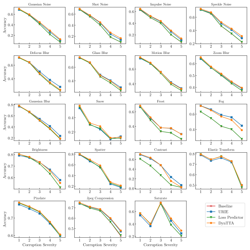
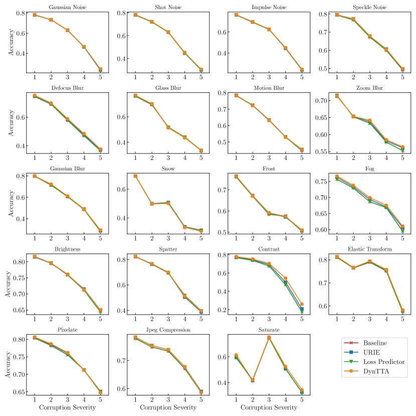
The results of the blind setting are shown in Figures 11-16. Several corruptions are more difficult for Loss Predictor to improve compared to other methods due to its small augmentation space. DynTTA outperforms the comparison methods in most experiments. In particular, in experiments where the classification model is Mixer-B16 w/AugMix and the corruptions are Speckle Noise and Contrast, DynTTA improves accuracy while other methods do not.