Abstract

The work is motivated by the Faraday cage effect. We consider the Helmholtz equation over a 3D-domain containing a thin heterogeneous interface of thickness $\delta\ll 1$. The layer has a $\delta-$periodic structure in the in-plane directions and is cylindrical in the third direction. The periodic layer has one connected component and a collection of isolated regions. The isolated region in the thin layer represents air or liquid, and the connected component represents a solid metal grid with a $\delta$ thickness. The main issue is created by the contrast of the coefficients in the air and in the grid and that the zero-order term has a complex-valued coefficient in the connected faze while a real-valued in the complement. An asymptotic analysis with respect to $\delta\to 0$ is provided, and the limit Helmholtz problem is obtained with the Dirichlet condition on the interface. The periodic unfolding method is used to find the limit.

Keywords: Homogenization; Helmholtz equations; Periodic unfolding; Thin structure
Mathematics Subject Classification (2010): 35B27, 35J50, 35J05, 74K10

1 Introduction

The work is motivated by a design of shielding textile material, that is, to design the periodic distance between yarns in the grid and the fiber thickness so that the material would act as a shield on a particular frequency. Therefore, in the appendix, we provide the explicit dependency of all the constants on geometric parameters. The main modeling issue here is the chosen contrast in the coefficients of the grid compared to the surrounding air or fluid. It is chosen as an order of $\delta^{-2}$, which leads to the complete shielding (zero Dirichlet boundary condition on the interface), while $\delta^{-1}$ leads to a partial shielding and depends on the grid design. The first case is focused in this article while the later case will be handled in another paper.

In this work, we consider the Helmholtz equation for two domains separated by a thin heterogeneous layer of the thickness $\delta\ll 1$. The layer has an $\delta-$ periodic structure in plane directions and is cylindrical with respect to the third direction, i.e., the in-plane structure is the same in all cross-sections. Two balks are connected by one of the components and another component is connected in the layer across the periodicity cells. The isolated region should represent an air or liquid and the connected plane grid with a thickness $\delta$ a solid, maybe metal. The first main issue is that the zero order term has a complex-valued coefficient in the connected faze (the grid) and a real-valued in the isolated regions and in the the bulk. The second issue is the contrast in the imaginary part of the zero-order-term-coefficient in the solid (may be metal), which relates as $\delta^{-2}$ to all other coefficients.

There is a huge literature on shielding problems. One can refer to [1, 11] concerning the acoustic wave propagation and the Maxwell equations have been extensively studied in [10, 18, 4, 5, 6, 17, 19, 13].

There exists a large number of papers devoted to the problems with thin layers of different structure. Depending on the relation between small parameters involved in geometry and stiffness of the layers, different limit problems can be obtained. In particular, [8] deals with the Neumann sieves of different thickness and sizes of inclusions. The articles [2, 3] consider the case of a thin stiff layer. A case of a soft homogeneous layer is discussed in [12, 14]. An interface problem with contrasting coefficients has been analysed in [20].

For the study of the limiting behaviour we use the periodic unfolding method, which was first introduced in [7], later developed in [9]. This method was used for different types of problems, particularly, problems for the thin layers in [8] and contact problems in the thin layer [14].

A regularization for the imaginary coefficient in front of the zero-order term was introduced and a uniform convergence with respect to this regularizing coefficient was proven. That is, we start with the regularized problem, show its convergence to the initial one, then pass to the limit in the regularized problem and then pass to the limit with the regularized parameter. Similar technique was used in [16] to regularize the contact problem with Coulomb’s friction.

The geometrical setting is similar to the one from [15], just in the complement to the domain the contrast in coefficients is considered.

The paper is organized in the following way. Section 2 provides the geometric setting and preliminary estimates of the solution. The wellposedness of the original problem and the convergence are studied in Section 3. Section 4 investigates the asymptotic analysis of the problem. Finally, the exact constants are given in the Appendix, those are expressed in terms of physical known constants, size of the domain, frequency and the source term. Those are important to design a shield with a particular frequency.

2 Geometrical setting and problem description

This section is devoted to describe the geometric structure of the domain and introduce the problem under consideration. In the Euclidean space $\mathbb{R}^{2}$ consider a domain ${\cal O}$ with a $C^{1,1}$ boundary and let $L>0$ be a fixed real number.
Define

$$\begin{array}[]{ll}\Omega_{\delta}^{+}&={\cal O}\times(\delta/2,L),\\ \Omega_{\delta}&={\cal O}\times(-\delta/2,\delta/2),\\ \Omega_{\delta}^{-}&={\cal O}\times(-L,-\delta/2),\end{array}$$ (2.1)

and

$$\Gamma ={\cal O}\times\{0\}.$$

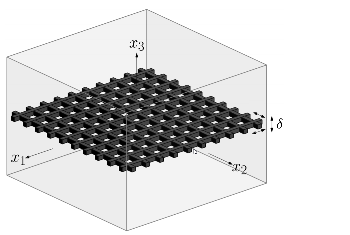
Figure 1: 3D-domain $\Omega$

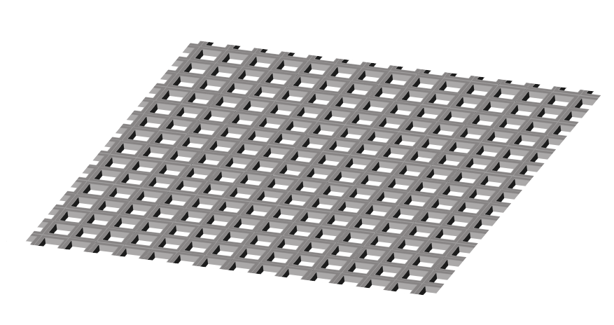
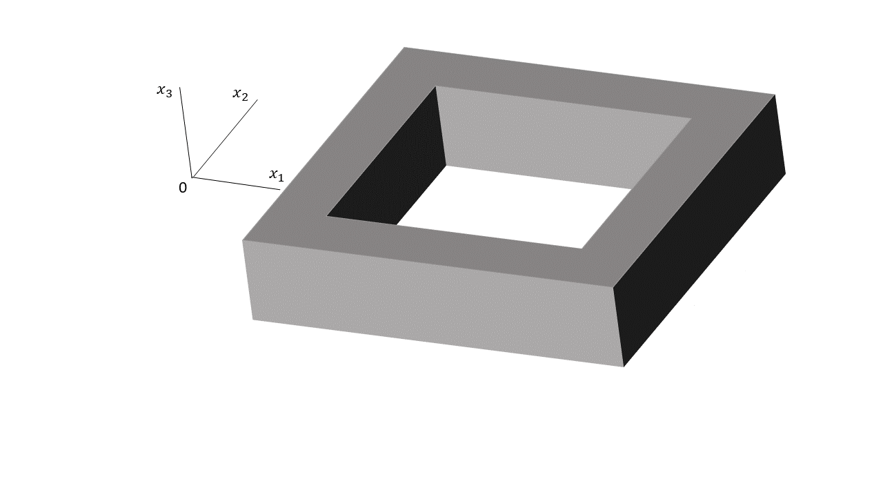
Figure 2: Grid structure and the reference cell.

Now, let us describe the thin layer. A model picture is given in Fig. 1 and 2. Here $\delta$ is a small parameter corresponding to the thickness of the layer and also the periodicity parameter in $x_{1}$ and $x_{2}$ directions.

The layer $\Omega_{\delta}$ has a periodic in-plane structure. The unit cell $Y$ is given by

$$Y\doteq\big{(}0,1\big{)}^{2}\times(-1/2,1/2)\subset{\mathbb{R}}^{3}.$$

Let $Y_{0}$ and $Y_{1}$ are two open subsets of $Y$. The set $Y_{0}$, as shown for example in Fig. 2, is an open set with Lipschitz boundary satisfying $Y_{0}\subset Y$, it will represent the periodic ”grid” and its complement $Y_{1}=Y\setminus\overline{Y_{0}}\not=\emptyset$ represents the air or material with less conductivity.

By scaling and translating $Y_{0}$ in $x_{1}$ and $x_{2}$ direction, we get the thin grid $\Omega_{\delta}^{i}$ as follows

$$\Xi_{\delta} =\big{\{}(\xi_{1},\xi_{2})\in{\mathbb{Z}}^{2}\;|\;\delta\big{(}\xi_{1}{\bf e}_{1}+\xi_{2}{\bf e}_{2}+Y\big{)}\subset\Omega\big{\}},$$ (2.2)

$$\Omega_{\delta}^{i} =\hbox{Interior}\bigcup_{\xi\in\Xi_{\delta}}\delta\big{(}\xi_{1}{\bf e}_{1}+\xi_{2}{\bf e}_{2}+\overline{Y_{0}}\big{)},$$ (2.3)

$$\widehat{{\cal O}}_{\delta} =\hbox{Interior}\bigcup_{\xi\in\Xi_{\delta}}\delta\big{(}\xi_{1}{\bf e}_{1}+\xi_{2}{\bf e}_{2}+[0,1]^{2}\big{)},$$ (2.4)

$$\Lambda_{\delta} ={\cal O}\setminus\widehat{{\cal O}}_{\delta}$$ (2.5)

where ${\bf e}_{1}$ and ${\bf e}_{2}$ are the canonical vectors ${\bf e}_{1}=(1,0,0)$ and ${\bf e}_{2}=(0,1,0)$. The grid/wire structure $\Omega_{\delta}^{i}$ is made up of a conducting material and holes between the grid, $\Omega_{\delta}^{*}$ is defined as

$$\Omega_{\delta}^{*}=\Omega_{\delta}\setminus\overline{\Omega_{\delta}^{i}}.$$

2.1 A preliminary result

Denote $H$ and $L$ two Hilbert spaces satisfying $H\subset L$. Below, we give a lemma with the exact computation of the constant.

Lemma 2.1.

[21] Let $a\;:\;H\times H\to{\mathbb{C}}$ be a continuous sesquilinear form satisfying

1. $|\Im(a(u,u))|\geq k_{1}\|u\|_{L}^{2}$ for all $u\in H$ for some $k_{1}>0$,

2. $|\Re(a(u,u))|\geq k_{2}\|u\|_{H}^{2}-k_{3}\|u\|_{L}^{2}$ for all $u\in H$ for some $k_{2},k_{3}>0$.

Then, there exists a constant $C>0$ which only depends on $k_{1},k_{2},$ and $k_{3}$ such that

$$|a(u,u)|\geq C\|u\|_{H}^{2},\qquad\forall u\in H.$$

The proof of this result with the exact constant is postponed to the appendix.

2.2 The Helmholtz problem

Let $\alpha,\beta,\omega\in{\mathbb{R}}^{+}$ be fixed. Let $M(\alpha,\beta,\Omega)$ be the set of all real valued matrix functions $A\in W^{1,\infty}(\Omega,{\mathbb{R}}^{3\times 3})$ such that

$$\alpha|\xi|^{2}\leq(A\xi,\xi),\qquad|A(\xi,\zeta)|\leq\beta|\xi||\zeta|$$

for all $(\xi,\zeta)\in{\mathbb{C}}^{3}\times{\mathbb{C}}^{3}$. Here $(\cdot,\cdot)$ is the usual ${\mathbb{C}}^{3}$ inner product.
Let us consider the following Helmholtz problem:

$$-{\text{div}}(A\nabla u_{\delta})-{\omega^{2}}\varepsilon_{\delta}u_{\delta} =i\omega f \text{ in }\Omega$$

$$u_{\delta} =0 \text{ on }\partial\Omega.$$

where $f\in L^{2}(\Omega,{\mathbb{C}})$ satisfies $\mathop{\rm supp}{f}\subset\overline{\Omega_{\delta}^{+}}$ and

$$\varepsilon_{\delta}(x)=\varepsilon_{1}+i\frac{\varepsilon_{2}}{\delta^{2}}\;\text{ if }\;x\in\Omega_{\delta}^{i},\qquad\varepsilon_{\delta}(x)=\varepsilon_{3}\;\text{ if }\;x\in\Omega\setminus\overline{\Omega_{\delta}^{i}}.$$ (2.6)

The $\varepsilon_{i}$’s are strictly positive constants.
The weak form of the above problem is given by

$$\left\{\begin{aligned} &\hbox{Find $u_{\delta}\in H^{1}_{0}(\Omega,{\mathbb{C}})$ such that }\\ &\int_{\Omega}A\nabla u_{\delta}\cdot\overline{\nabla\psi}\,dx-\omega^{2}\int_{\Omega}\varepsilon_{\delta}u_{\delta}\cdot\overline{\psi}\,dx=i\omega\int_{\Omega}f\cdot\overline{\psi}\,dx,~{}~{}~{}~{}\forall\psi\in H^{1}_{0}(\Omega,{\mathbb{C}}).\end{aligned}\right.$$ (2.7)

The following lemma recalls a classical result which will be used in the upcoming sections.

Lemma 2.2.

For every $v\in H^{1}(\Omega_{\delta},{\mathbb{C}})$ one has

$$\|v\|_{L^{2}(\Omega_{\delta},{\mathbb{C}})}\leq C\Big{(}\|v\|_{L^{2}(\Omega^{i}_{\delta},{\mathbb{C}})}+\delta\|\nabla v\|_{L^{2}(\Omega_{\delta},{\mathbb{C}})}\Big{)},$$ (2.8)

$$\delta\|v\|^{2}_{L^{2}(\Gamma,{\mathbb{C}})}\leq C\Big{(}\|v\|^{2}_{L^{2}(\Omega_{\delta},{\mathbb{C}})}+\delta^{2}\|\nabla v\|^{2}_{L^{2}(\Omega_{\delta},{\mathbb{C}})}\Big{)}.$$

The constant does not depend on $\delta$.

Proof.

Note that for $\phi\in H^{1}(Y,{\mathbb{C}})$

$$\|\phi\|_{L^{2}(Y,{\mathbb{C}})}\leq C\Big{(}\|\phi\|_{L^{2}(Y_{0},{\mathbb{C}})}+\|\nabla\phi\|_{L^{2}(Y,{\mathbb{C}})}\Big{)}.$$ (2.9)

This is a classical inequality, one can proceed by contradiction and use the compact embedding of $L^{2}(Y,{\mathbb{C}})$ in $H^{1}(Y,{\mathbb{C}})$ for a simple proof. Then, use a change of variables to give the estimates in the $\delta$-cells, add the obtained inequalities to get (2.8)₁, then prove (2.8)₂. ∎

3 Existence of the solution to the Helmholtz problem

We endow $L^{2}(\Omega,{\mathbb{C}})$ with the scalar product

$$\langle u,v\rangle=\int_{\Omega}\,u\,\overline{v}\,dx\hbox{ }.$$

Denote

$$\langle A\nabla u,\nabla v\rangle=\int_{\Omega}A\nabla u\cdot\overline{\nabla v}\,dx\quad\hbox{ for }u,v\in H^{1}(\Omega,{\mathbb{C}})$$

and

$$\varepsilon^{\delta}=\varepsilon_{1}\quad\hbox{a.e. in }\;\Omega^{i}_{\delta},\qquad\varepsilon^{\delta}=\varepsilon_{3}\quad\hbox{a.e. in }\;\Omega\setminus\overline{\Omega^{i}_{\delta}}.$$

The wellposedness of the Helmholtz problem (2.7) is proved in the following theorem.

Theorem 3.1.

Assume that $\omega^{2}\varepsilon_{3}$ is not an eigenvalue of $-\text{div }(A\nabla)$ in $H^{1}_{0}(\Omega^{+},{\mathbb{C}})$. Then, there exist two strictly positive constants $\delta_{0}$ and $C$ such that for every $\delta\in(0,\delta_{0}]$ and every $f\in L^{2}(\Omega,{\mathbb{C}})$, problem (2.7) admits a unique solution $u_{\delta}\in H^{1}_{0}(\Omega,{\mathbb{C}})$ satisfying

$$\|u_{\delta}\|_{H^{1}(\Omega,{\mathbb{C}})}\leq{C}\|f\|_{L^{2}(\Omega,{\mathbb{C}})}.$$ (3.1)

We remark about the constant in the appendix.

Proof.

Step 1. In this step we prove that there exists $\delta_{0}>0$ such that: if $u_{\delta}\in H^{1}_{0}(\Omega,{\mathbb{C}})$, $\delta\in(0,\delta_{0}]$, satisfies

$$\langle A\nabla u_{\delta},\nabla\phi\rangle-\omega^{2}\langle\varepsilon^{\delta}u_{\delta},\phi\rangle-i\omega^{2}\int_{\Omega_{\delta}^{i}}{\varepsilon_{2}\over\delta^{2}}\,u_{\delta}\,\overline{\phi}\,dx=0,\qquad\forall\phi\in H^{1}_{0}(\Omega,{\mathbb{C}})$$ (3.2)

then $u_{\delta}=0$.
First observe that $u_{\delta}$ satisfying (3.2) also satisfies $u_{\delta}=0$ a.e. in $\Omega^{i}_{\delta}$.
We proceed by contradiction. Suppose that for every $n\in{\mathbb{N}}\setminus\{0\}$ there exist $\delta_{n}\in(0,1/n]$ and $u_{\delta_{n}}\in H^{1}_{0}(\Omega,{\mathbb{C}})$ such that

$$\|u_{\delta_{n}}\|_{L^{2}(\Omega,{\mathbb{C}})}=1,\quad u_{\delta_{n}}=0\ \ \hbox{a.e. in }\ \ \Omega^{i}_{\delta_{n}},\quad\langle A\nabla u_{\delta_{n}},\nabla\phi\rangle=\omega^{2}\langle\varepsilon^{\delta_{n}}u_{\delta_{n}},\phi\rangle,\qquad\forall\phi\in H^{1}_{0}(\Omega,{\mathbb{C}}).$$

Set

$$v_{\delta_{n}}={u_{\delta_{n}}\over\|u_{\delta_{n}}\|_{L^{2}(\Omega,{\mathbb{C}})}}.$$

By (3.2), we have (as $A\in M(\alpha,\beta,\Omega)$)

$$\|\nabla v_{\delta_{n}}\|_{L^{2}(\Omega,{\mathbb{C}})}^{2}\leq C$$

where $\displaystyle C=\omega^{2}\frac{\max\{\varepsilon_{1},\varepsilon_{3}\}}{\alpha}$ is independent of $\delta_{n}$. Then, up to a subsequence one has

$$v_{\delta_{n}}\rightharpoonup v\;\hbox{weakly in }H^{1}_{0}(\Omega,{\mathbb{C}}),\qquad v_{\delta_{n}}\to v\;\hbox{strongly in }L^{2}(\Omega,{\mathbb{C}}).$$

The strong convergence in $L^{2}(\Omega,{\mathbb{C}})$ implies $\|v\|_{L^{2}(\Omega,{\mathbb{C}})}=1$. Using (2.8)_1,2, we obtain that $v=0$ a.e. on $\Gamma$ (since $\|v_{\delta_{n}}\|^{2}_{L^{2}(\Gamma)}\leq C\sqrt{\delta_{n}}$) and thus

$$\langle A\nabla v,\nabla\phi\rangle=\omega^{2}\varepsilon_{3}\langle v,\phi\rangle\qquad\forall\phi\in H^{1}_{0}(\Omega^{\pm},{\mathbb{C}}).$$ (3.3)

This means that $\omega^{2}\varepsilon_{3}$ is an eigenvalue and $v$ an eigenfunction of $-{\text{div}}(A\nabla)$ in $H^{1}_{0}(\Omega^{\pm},{\mathbb{C}})$.

$$-{\text{div}}(A\nabla v)=\omega^{2}\varepsilon_{3}v\qquad\hbox{in }\Omega^{\pm},\qquad v\in H^{1}_{0}(\Omega^{\pm},{\mathbb{C}}).$$

This contradicts the assumption of the theorem. Hence, the claim of this step is proved.
In the following steps we assume $\delta\in(0,\delta_{0}]$.
Step 2. In this step we fix $\delta\in(0,\delta_{0}]$ and we prove that problem (2.7) admits solutions.
Set

$$\varepsilon^{\delta}_{\theta}={\varepsilon_{2}\over\delta^{2}}\quad\hbox{a.e. in }\;\Omega^{i}_{\delta},\qquad\varepsilon^{\delta}_{\theta}=\theta\quad\hbox{a.e. in }\;\Omega\setminus\overline{\Omega^{i}_{\delta}},\\$$

where $\theta$ is a strictly positive constant less than $\displaystyle{\varepsilon_{2}\over\delta^{2}}$.
We consider the following variational problem:

$$\left\{\begin{aligned} &\hbox{Find }\ \ u^{\theta}_{\delta}\in H^{1}_{0}(\Omega,{\mathbb{C}})\;\hbox{such that }\\ &\langle A\nabla u^{\theta}_{\delta},\nabla\phi\rangle-\omega^{2}\langle\varepsilon^{\delta}u^{\theta}_{\delta},\phi\rangle-i\omega^{2}\int_{\Omega}\varepsilon_{\theta}^{\delta}\,u^{\theta}_{\delta}\,\overline{\phi}\,dx=i\omega\int_{\Omega}f\,\overline{\phi}\,dx,\qquad\forall\phi\in H^{1}_{0}(\Omega,{\mathbb{C}}).\end{aligned}\right.$$ (3.4)

Define $B^{\delta}_{\theta}\;:\;H^{1}_{0}(\Omega,{\mathbb{C}})\times H^{1}_{0}(\Omega,{\mathbb{C}})\to{\mathbb{C}}$ by

$$B^{\delta}_{\theta}(u,v)\doteq\langle A\nabla u,\nabla v\rangle-\omega^{2}\langle\varepsilon^{\delta}u,v\rangle-i\omega^{2}\int_{\Omega}\varepsilon_{\theta}^{\delta}\,u\,\overline{v}\,dx.$$

Note that

$$|\Im(B^{\delta}_{\theta}(u,u))|\geq\omega^{2}\theta\|u\|^{2}_{L^{2}(\Omega,{\mathbb{C}})},\qquad|\Re(B^{\delta}_{\theta}(u,u))|\geq\alpha\|u\|_{H^{1}(\Omega,{\mathbb{C}})}^{2}-{\tau\omega^{2}}\|u\|^{2}_{L^{2}(\Omega,{\mathbb{C}})}.$$

where the constant $\tau=\max\{\varepsilon_{1},\varepsilon_{3}\}$. Besides, we have

$$|B^{\delta}_{\theta}(u,\phi)| \leq\beta|\langle u,\phi\rangle_{H}|+\omega^{2}|\langle\varepsilon^{\delta}u,\phi\rangle|+\omega^{2}\int_{\Omega}\varepsilon_{\theta}^{\delta}\,|u\,\overline{\phi}|\,dx\leq C(\delta)\|u\|_{H}\|\phi\|_{H}.$$

Hence by Lemma 2.1 ($H=H^{1}_{0}(\Omega,{\mathbb{C}})$, $L=L^{2}(\Omega,{\mathbb{C}})$), we have that $B^{\delta}_{\theta}$ is elliptic and bounded, that is

$$|B^{\delta}_{\theta}(u,u)|\geq C^{\prime}(\delta,\theta)\|u\|_{H}^{2}.$$ (3.5)

The explicit value of $C^{\prime}(\delta,\theta)$ is remarked in Section 5, therefore for $\theta$ small enough (less than a strictly positive constant $C(\alpha,\tau,\omega)$) one has $\displaystyle C^{\prime}(\delta,\theta)={\alpha\theta\over\tau}$. Hence, for $\theta$ small enough, by Lax-Milgram, we have a unique solution $u^{\theta}_{\delta}$ of the problem (3.4) and

$$\|\nabla u^{\theta}_{\delta}\|_{L^{2}(\Omega,{\mathbb{C}})}\leq\frac{\tau\omega}{\alpha\theta}||f||_{L^{2}(\Omega,{\mathbb{C}})},\qquad\|u^{\theta}_{\delta}\|_{H^{1}_{0}(\Omega,{\mathbb{C}})}\leq\frac{\tau\omega~{}diam(\Omega)}{\alpha\theta}||f||_{L^{2}(\Omega,{\mathbb{C}})},$$

where $diam(\Omega)$ comes from the Poincaré inequality.
Claim 1: There exists a constant $C(\delta,f)$ such that for $\theta$ small enough (less than ${\varepsilon_{2}/\delta^{2}}$ and $C(\alpha,\tau,\omega)$) $\|u_{\delta}^{\theta}\|_{L^{2}(\Omega,{\mathbb{C}})}\leq C(\delta,f)$.
First, let us replace the test function $\phi$ in (3.2) with the solution to get

$$\langle A\nabla u^{\theta}_{\delta},\nabla u^{\theta}_{\delta}\rangle-i\omega^{2}\int_{\Omega}\varepsilon_{\theta}^{\delta}\,|u^{\theta}_{\delta}|^{2}\,dx=i\omega\int_{\Omega}f\,\overline{u_{\delta}^{\theta}}\,dx+\omega^{2}\int_{\Omega}\varepsilon^{\delta}|u^{\theta}_{\delta}|^{2}\,dx.$$ (3.6)

By equating the real part one arrives at

$$\langle A\nabla u^{\theta}_{\delta},\nabla u^{\theta}_{\delta}\rangle =-\omega\int_{\Omega}\Im(f\,\overline{u_{\delta}^{\theta}})\,dx+\omega^{2}\int_{\Omega}\varepsilon^{\delta}|u^{\theta}_{\delta}|^{2}\,dx$$

and then

$$\alpha\|\nabla u^{\theta}_{\delta}\|_{L^{2}(\Omega,{\mathbb{C}})}^{2} \leq|\langle A\nabla u^{\theta}_{\delta},\nabla u^{\theta}_{\delta}\rangle|\leq\omega\int_{\Omega}|f\,\overline{u_{\delta}^{\theta}}|\,dx+\omega^{2}\int_{\Omega}\varepsilon^{\delta}|u^{\theta}_{\delta}|^{2}\,dx$$ (3.7)

$$\leq\omega\|f\|_{L^{2}(\Omega,{\mathbb{C}})}\|u^{\theta}_{\delta}\|_{L^{2}(\Omega,{\mathbb{C}})}+\omega^{2}\tau\|u^{\theta}_{\delta}\|_{L^{2}(\Omega,{\mathbb{C}})}^{2}.$$

Now, $f$ and $\delta\in(0,\delta_{0}]$ being fixed, we prove the claim by contradiction. If there exists a sequence $\{\theta_{k}\}_{k}$ converging to 0 such that $\|u^{\theta_{k}}_{\delta}\|_{L^{2}(\Omega,{\mathbb{C}})}\to+\infty$. Set

$$v^{\theta_{k}}_{\delta}={u^{\theta_{k}}_{\delta}\over\|u^{\theta_{k}}_{\delta}\|_{L^{2}(\Omega,{\mathbb{C}})}}.$$

By (3.7), we have

$$\|\nabla v^{\theta_{k}}_{\delta}\|_{L^{2}(\Omega,{\mathbb{C}})}^{2}={\|\nabla u^{\theta_{k}}_{\delta}\|_{L^{2}(\Omega,{\mathbb{C}})}^{2}\over\|u^{\theta_{k}}_{\delta}\|_{L^{2}(\Omega,{\mathbb{C}})}^{2}}\leq C$$

where $\displaystyle C=\frac{\omega}{\alpha}(1+\omega\tau)$ is independent of $\theta_{k}$ (as $\displaystyle\frac{\|f\|_{L^{2}(\Omega,{\mathbb{C}})}}{\|u_{\delta}^{\theta_{k}}\|_{L^{2}(\Omega,{\mathbb{C}})}}\ll 1$). Thus $v^{\theta_{k}}_{\delta}$ is bounded in $H^{1}_{0}(\Omega,{\mathbb{C}})$ independent of $\theta_{k}$. Then, up to a subsequence one has

$$v^{\theta_{k}}_{\delta}\rightharpoonup v_{\delta}\;\hbox{weakly in }H^{1}_{0}(\Omega,{\mathbb{C}}),\qquad v^{\theta_{k}}_{\delta}\to v_{\delta}\;\hbox{strongly in }L^{2}(\Omega,{\mathbb{C}}).$$

Let us divide the equation (3.4) by $\|u^{\theta_{k}}_{\delta}\|_{L^{2}(\Omega,{\mathbb{C}})}$ to get

$$\langle A\nabla v^{\theta_{k}}_{\delta},\nabla\phi\rangle-\omega^{2}\langle\varepsilon^{\delta}v^{\theta_{k}}_{\delta},\phi\rangle-i\omega^{2}\int_{\Omega}\varepsilon_{\theta_{k}}^{\delta}\,v^{\theta_{k}}_{\delta}\,\overline{\phi}\,dx={i\omega\over\|u^{\theta_{k}}_{\delta}\|_{L^{2}(\Omega,{\mathbb{C}})}}\int_{\Omega}f\,\overline{\phi}\,dx,\qquad\forall\phi\in H^{1}_{0}(\Omega,{\mathbb{C}}).$$

Now, pass to the limit as $\theta_{k}\to 0$ to get

$$\langle A\nabla v_{\delta},\nabla\phi\rangle-\omega^{2}\langle\varepsilon^{\delta}v_{\delta},\phi\rangle-i\omega^{2}\int_{\Omega_{\delta}^{i}}{\varepsilon_{2}\over\delta^{2}}\,v_{\delta}\,\overline{\phi}\,dx=0\qquad\forall\phi\in H^{1}_{0}(\Omega,{\mathbb{C}}).$$ (3.8)

As $\|v^{\theta_{k}}_{\delta}\|_{L^{2}(\Omega,{\mathbb{C}})}=1$ and the strong convergence in $L^{2}(\Omega,{\mathbb{C}})$, we have $\|v_{\delta}\|_{L^{2}(\Omega,{\mathbb{C}})}=1$. So by Step 1, $v_{\delta}=0$ which is a contradiction.
As a consequence one has

$$\forall\theta\in\big{(}0,\min\{{\varepsilon_{2}/\delta^{2}},\,C(\alpha,\tau,\omega)\}\big{]},\qquad\|u_{\delta}^{\theta}\|_{L^{2}(\Omega,{\mathbb{C}})}\leq C\big{(}\delta,f).$$

This proves the Claim 1. Thus $\|\nabla u^{\theta}_{\delta}\|_{L^{2}(\Omega,{\mathbb{C}})}\leq C(\delta,f)$.
Now, let $\theta_{k}$ be a sequence converging to 0, such that $u^{\theta_{k}}_{\delta}\rightharpoonup u_{\delta}$ weakly in $H^{1}_{0}(\Omega,{\mathbb{C}})$. Hence, passing to the limit, the equation (3.4) becomes

$$\langle A\nabla u_{\delta},\nabla\phi\rangle-\omega^{2}\langle\varepsilon^{\delta}u_{\delta},\phi\rangle-i\omega^{2}\int_{\Omega_{\delta}^{i}}{\varepsilon_{2}\over\delta^{2}}\,u_{\delta}\,\overline{\phi}\,dx=i\omega\int_{\Omega}f\,\overline{\phi}\,dx,\qquad\forall\phi\in H^{1}_{0}(\Omega,{\mathbb{C}})$$ (3.9)

which proves that (2.7) admits solutions. Then, Step 1 ensures that (2.7) admits a unique solution.
Step 3. In this step we prove that the unique solution of problem (2.7) satisfies

$$\|u_{\delta}\|_{H^{1}(\Omega,{\mathbb{C}})}\leq C\|f\|_{L^{2}(\Omega,{\mathbb{C}})}.$$

Claim 2: There exists a constant $C>0$ such that

$$\sup_{\delta\in(0,\delta_{0}],\;f\in L^{2}(\Omega,{\mathbb{C}}),\,\|f\|_{L^{2}(\Omega,{\mathbb{C}})}=1}\|u_{\delta}(f)\|_{L^{2}(\Omega,{\mathbb{C}})}\leq C.$$ (3.10)

Here, $u_{\delta}(f)$ denote the unique solution to (2.7).
Suppose not, then there exists a sequence $\{\delta_{k}\}_{k\in{\mathbb{N}}}$ converging to $\delta^{*}\in[0,\delta_{0}]$ and $f_{k}\in L^{2}(\Omega,{\mathbb{C}})$ with $\|f_{k}\|_{L^{2}(\Omega,{\mathbb{C}})}=1$, such that $\displaystyle\lim_{k\to+\infty}\|u_{\delta_{k}}\|_{L^{2}(\Omega,{\mathbb{C}})}\to+\infty$.
Case 1: $\delta^{*}=0$. Now, (2.7) gives

$$\langle A\nabla u_{\delta_{k}},\nabla u_{\delta_{k}}\rangle-\omega^{2}\int_{\Omega}\varepsilon^{\delta_{k}}|u_{\delta_{k}}|^{2}\,dx-i\omega^{2}\int_{\Omega_{\delta_{k}}^{i}}{\varepsilon_{2}\over{\delta_{k}}^{2}}\,|u_{\delta_{k}}|^{2}\,dx=i\omega\int_{\Omega}f_{k}\overline{u_{\delta_{k}}}\,dx.$$ (3.11)

By considering the imaginary parts, one gets

$$\omega^{2}\int_{\Omega_{\delta_{k}}^{i}}{\varepsilon_{2}\over{\delta_{k}}^{2}}\,|u_{\delta_{k}}|^{2}\,dx\leq\omega\int_{\Omega}|\Re(f_{k}\overline{u_{\delta_{k}}})|\,dx\leq\omega\|f_{k}\|_{L^{2}(\Omega,{\mathbb{C}})}\|u_{\delta_{k}}\|_{L^{2}(\Omega,{\mathbb{C}})}\leq C\|u_{\delta_{k}}\|_{L^{2}(\Omega,{\mathbb{C}})}.$$ (3.12)

Set

$$v_{\delta_{k}}={u_{\delta_{k}}\over\|u_{\delta_{k}}\|_{L^{2}(\Omega,{\mathbb{C}})}}.$$

Thus one gets

$$\omega^{2}\int_{\Omega_{\delta_{k}}^{i}}{\varepsilon_{2}\over{\delta_{k}}^{2}}\,|v_{\delta_{k}}|^{2}\,dx\leq{C\over\|u_{\delta_{k}}\|_{L^{2}(\Omega,{\mathbb{C}})}},$$ (3.13)

and hence the LHS converges to 0.
The real part gives

$$\|\nabla v_{\delta_{k}}\|_{L^{2}(\Omega,{\mathbb{C}})} \leq C.$$ (3.14)

Then, from Lemma 2.2 and the above estimates we get

$$\|v_{\delta_{k}}\|_{L^{2}(\Gamma,{\mathbb{C}})}\leq C\sqrt{\delta_{k}}$$

where $C$ is independent of $\delta_{k}$. So, up to a subsequence there exists $v\in H^{1}_{0}(\Omega,{\mathbb{C}})$ such that as $k\to\infty$

$$v_{\delta_{k}}\rightharpoonup v\,\quad\text{weakly in }H^{1}(\Omega,{\mathbb{C}}),\qquad v_{\delta_{k}}\to v\;\hbox{strongly in }L^{2}(\Omega,{\mathbb{C}}).$$

The strong convergence in $L^{2}(\Omega,{\mathbb{C}})$ implies $\|v\|_{L^{2}(\Omega,{\mathbb{C}})}=1$. Moreover, we have $v=0$ a.e. on $\Gamma$.
Let us divide the equation (2.7) by $\|u_{\delta_{k}}\|_{L^{2}(\Omega,{\mathbb{C}})}$ to get

$$\langle A\nabla v_{\delta_{k}},\nabla\phi\rangle-\omega^{2}\langle\varepsilon^{\delta_{k}}v_{\delta_{k}},\phi\rangle-i\omega^{2}\int_{\Omega_{\delta_{k}}^{i}}{\varepsilon_{2}\over\delta^{2}_{k}}\,v_{\delta_{k}}\,\overline{\phi}\,dx={i\omega\over\|u_{\delta_{k}}\|_{L^{2}(\Omega,{\mathbb{C}})}}\int_{\Omega}f_{k}\,\overline{\phi}\,dx,\qquad\forall\phi\in H^{1}_{0}(\Omega,{\mathbb{C}}).$$ (3.15)

Let $\phi^{+}$ (resp. $\phi^{-}$) be in ${\cal D}(\Omega^{+},{\mathbb{C}})$ (resp. ${\cal D}(\Omega^{-},{\mathbb{C}})$). If $\delta_{k}$ is sufficiently small, one has

$$\int_{\Omega^{+}}A\nabla v_{\delta_{k}}\cdot\overline{\nabla\phi^{+}}\,dx-\omega^{2}\int_{\Omega^{+}}\varepsilon_{3}v_{\delta_{k}}\overline{\phi^{+}}\,dx=i\omega{1\over\|u_{\delta_{k}}\|_{L^{2}(\Omega,{\mathbb{C}})}}\int_{\Omega^{+}}f\overline{\phi^{+}}\,dx,$$

(resp. $$\int_{\Omega^{-}}A\nabla v_{\delta_{k}}\cdot\overline{\nabla\phi^{-}}\,dx-\omega^{2}\int_{\Omega^{-}}\varepsilon_{3}v_{\delta_{k}}\overline{\phi^{-}}\,dx=0\;\hbox{).}$$

Passing to the limit yield

$$\int_{\Omega^{+}}A\nabla v\cdot\nabla\overline{\phi}\,dx+\omega^{2}\varepsilon_{3}\int_{\Omega^{+}}v\overline{\phi}\,dx=0,\qquad\forall\phi^{+}\in{\cal D}(\Omega^{+},{\mathbb{C}})$$

and

$$\int_{\Omega^{-}}A\nabla v\cdot\nabla\overline{\phi}\,dx+\omega^{2}\varepsilon_{3}\int_{\Omega^{-}}v\overline{\phi}\,dx=0,\qquad\forall\phi^{-}\in{\cal D}(\Omega^{-},{\mathbb{C}}).$$ (3.16)

A density argument gives

$$\langle A\nabla v,\nabla\phi\rangle-\omega^{2}\varepsilon_{3}\langle v,\phi\rangle=0\qquad\forall\phi\in H^{1}_{0}(\Omega^{\pm},{\mathbb{C}})$$

where $v\in H^{1}_{0}(\Omega^{\pm},{\mathbb{C}})$ which, thanks to Step 1, contradicts the hypothesis of the theorem.
Case 2: $\delta^{*}\neq 0$. As above (see the estimate (3.14)) we show that the sequence $\{v_{\delta_{k}}\}_{k}$ is uniformly bounded in $H^{1}_{0}(\Omega,{\mathbb{C}})$. So, up to a subsequence there exists $v_{\delta^{*}}\in H^{1}_{0}(\Omega,{\mathbb{C}})$ such that as $k\to\infty$

$$v_{\delta_{k}}\rightharpoonup v_{\delta^{*}}\,\quad\text{weakly in }H^{1}_{0}(\Omega,{\mathbb{C}})\,\text{ and }v_{\delta_{k}}\to v_{\delta^{*}}\,\quad\text{strongly in }L^{3}(\Omega,{\mathbb{C}}).$$

The second convergence is due to Rellich-Kondrasov Theorem. The imaginary part of the energy gives

$$\int_{\Omega_{\delta_{k}}^{i}}|v_{\delta_{k}}|^{2}\,dx\leq{C\delta_{k}^{2}\over\|u_{\delta_{k}}\|_{L^{2}(\Omega,{\mathbb{C}})}}.$$

Note that

$$\chi_{\Omega_{\delta_{k}}^{i}}(x)\to\chi_{\Omega_{\delta^{*}}^{i}}(x)\;\;\hbox{for a.e. $x\in\Omega$ }$$

where $\chi_{D}$ denotes the characteristic function of the set $D$. So, the above estimate and convergence imply that

$$\chi_{\Omega_{\delta_{k}}^{i}}v_{\delta_{k}}\to 0\,\quad\text{strongly in }L^{2}(\Omega,{\mathbb{C}}).$$

Since the sequence $\{v_{\delta_{k}}\}_{k}$ converges to $v_{\delta^{*}}$ strongly in $L^{3}(\Omega,{\mathbb{C}})$, we obtain $v_{\delta^{*}}=0$ a.e. in $\Omega^{i}_{\delta^{*}}$.
Besides, we get that $\|v_{\delta_{k}}\|_{L^{2}(\Omega,{\mathbb{C}})}=1$ for all $k$ and hence $\|v_{\delta^{*}}\|_{L^{2}(\Omega_{\delta^{*}}^{*})}=1$ as $v_{\delta_{k}}$ converges to $v_{\delta^{*}}$ strongly in $L^{2}(\Omega,{\mathbb{C}})$. Finally, passing to the limit in (3.15), we obtain that $v_{\delta^{*}}$ satisfies

$$\langle A\nabla v_{\delta^{*}},\nabla\phi\rangle_{L^{2}(\Omega_{\delta^{*}}^{*},{\mathbb{C}}^{3})}-\omega^{2}\varepsilon_{3}\langle v_{\delta^{*}},\phi\rangle_{L^{2}(\Omega_{\delta^{*}}^{*},{\mathbb{C}})}=0\qquad\forall\phi\in H^{1}_{0}(\Omega_{\delta^{*}}^{*},{\mathbb{C}}).$$ (3.17)

Due to the result of Step 1, we have $v_{\delta^{*}}=0$ which is a contradiction. This completes the theorem. ∎

Corollary 3.1.

For every $\delta\in(0,\delta_{0}]$ and every $f\in L^{2}(\Omega,{\mathbb{C}})$, the solution $u_{\delta}\in H_{0}^{1}(\Omega,{\mathbb{C}})$ to the problem (2.7) satisfies

$$\|u_{\delta}\|_{H^{1}(\Omega,{\mathbb{C}})}+\delta^{-1}\|u_{\delta}\|_{L^{2}(\Omega_{\delta}^{i})}\leq C\|f\|_{L^{2}(\Omega,{\mathbb{C}})}$$ (3.18)

where $C>0$ is independent of $\delta$ and $f$.

Proof.

The imaginary part of the energy of (3.9) gives

$${\varepsilon_{2}\over{\delta}^{2}}\int_{\Omega_{\delta}^{i}}\,|u_{\delta}|^{2}\,dx\leq\omega\int_{\Omega}|\Re(f\overline{u_{\delta}})|\,dx\leq\omega\|f\|_{L^{2}(\Omega,{\mathbb{C}})}\|u_{\delta}\|_{L^{2}(\Omega,{\mathbb{C}})}.$$

Thus one gets

$$\delta^{-2}\|u_{\delta}\|^{2}_{L^{2}(\Omega_{\delta}^{i},{\mathbb{C}})}\leq{1\over\omega\varepsilon_{2}}\|f\|_{L^{2}(\Omega,{\mathbb{C}})}\|u_{\delta}\|_{L^{2}(\Omega,{\mathbb{C}})}\leq C\|f\|^{2}_{L^{2}(\Omega,{\mathbb{C}})}.$$ (3.19)

∎

Lemma 2.2 and estimates (3.18) yield

$$\|u_{\delta}\|_{L^{2}(\Omega_{\delta},{\mathbb{C}})}\leq C\delta\|f\|_{L^{2}(\Omega,{\mathbb{C}})},\qquad\|\nabla u_{\delta}\|_{L^{2}(\Omega_{\delta},{\mathbb{C}})}\leq C\|f\|_{L^{2}(\Omega,{\mathbb{C}})},\qquad\|u_{\delta}\|_{L^{2}(\Gamma,{\mathbb{C}})}\leq C\sqrt{\delta}\|f\|_{L^{2}(\Omega,{\mathbb{C}})}.$$ (3.20)

Proposition 3.1.

There exists $u\in H^{1}_{0}(\Omega,{\mathbb{C}})$ such that

$$u_{\delta}\rightharpoonup u\quad\hbox{weakly in }H^{1}_{0}(\Omega,{\mathbb{C}}).$$ (3.21)

Moreover, $u=0$ a.e. in $\Omega^{-}$ and $u$ restricted to $\Omega^{+}$ belongs to $H^{1}_{0}(\Omega^{+},{\mathbb{C}})$ and is the unique solution of

$$\int_{\Omega^{+}}A\nabla u\cdot\overline{\nabla\phi}\,dx-\omega^{2}\varepsilon_{3}\int_{\Omega^{+}}u\,\overline{\phi}\,dx=i\omega\int_{\Omega^{+}}f\,\overline{\phi}\,dx,\qquad\forall\phi\in H^{1}_{0}(\Omega^{+},{\mathbb{C}}).$$ (3.22)

Proof.

First, there exist a subsequence of $\{\delta\}$, still denoted $\{\delta\}$, and $u\in H^{1}_{0}(\Omega,{\mathbb{C}})$ such that

$$u_{\delta}\rightharpoonup u\quad\hbox{weakly in }H^{1}_{0}(\Omega,{\mathbb{C}}).$$

Observe that due to (3.20)₃, one has $u=0$ a.e. on $\Gamma$.
Let $\psi^{+}$ (resp. $\psi^{-}$) be in ${\cal D}(\Omega^{+},{\mathbb{C}})$ (resp. ${\cal D}(\Omega^{-},{\mathbb{C}})$). For every $\delta$ sufficiently small, one has

$$\int_{\Omega^{+}}A\nabla u_{\delta}\cdot\overline{\nabla\psi^{+}}\,dx-\omega^{2}\varepsilon_{3}\int_{\Omega^{+}}u_{\delta}\overline{\psi^{+}}\,dx=i\omega\int_{\Omega^{+}}f\overline{\psi^{+}}\,dx,$$

(resp. $$\int_{\Omega^{-}}A\nabla u_{\delta}\cdot\overline{\nabla\psi^{-}}\,dx-\omega^{2}\varepsilon_{3}\int_{\Omega^{-}}u_{\delta}\overline{\psi^{-}}\,dx=0\;\hbox{).}$$

Passing to the limit yield

$$\int_{\Omega^{+}}A\nabla u\cdot\nabla\overline{\psi}\,dx-\omega^{2}\varepsilon_{3}\int_{\Omega^{+}}u\overline{\psi}\,dx=i\omega\int_{\Omega^{+}}f\overline{\psi}\,dx,\qquad\forall\psi^{+}\in{\cal D}(\Omega^{+},{\mathbb{C}})$$

and

$$\int_{\Omega^{-}}A\nabla u\cdot\nabla\overline{\psi}\,dx-\omega^{2}\varepsilon_{3}\int_{\Omega^{-}}u\overline{\psi}\,dx=0,\qquad\forall\psi^{-}\in{\cal D}(\Omega^{-},{\mathbb{C}}).$$ (3.23)

A density argument gives (3.22). This gives the existence, the uniqueness is followed by a similar arguments in Step 1 of Theorem 3.1. ∎

As the boundary of $\cal O$ is ${\cal C}^{1,1}$, we have $u_{|\Omega^{+}}$ belongs to $H^{1}_{0}(\Omega^{+},{\mathbb{C}})\cap H^{2}(\Omega^{+},{\mathbb{C}})$ and

$$\|u\|_{H^{2}(\Omega^{+},{\mathbb{C}})}\leq C\|u\|_{H^{1}(\Omega^{+},{\mathbb{C}})}\leq C\|f\|_{L^{2}(\Omega,{\mathbb{C}})}.$$

We recall the following classical result: for every $\phi\in H^{1}({\Omega^{+}})$ one has

$$\|\phi\|_{L^{2}({\cal O}\times(0,\delta/2),{\mathbb{C}})}^{2}\leq\delta\|\phi\|_{L^{2}(\Omega^{+},{\mathbb{C}})}^{2}+\delta^{2}\left\|\frac{\partial\phi}{\partial x_{3}}\right\|_{L^{2}(\Omega^{+},{\mathbb{C}})}^{2}.$$ (3.24)

As a consequence, the solution to problem (3.22) satisfies (remind that $\nabla u\in H^{1}(\Omega^{+},{\mathbb{C}}^{3})$, $\nabla u=0$ in $\Omega^{-}$ and $u=0$ a.e. on $\Gamma$)

$$\|\nabla u\|_{L^{2}(\Omega_{\delta},{\mathbb{C}})} =\|\nabla u\|_{L^{2}({\cal O}\times(0,\delta/2),{\mathbb{C}})}\leq C\delta^{1/2}\|u\|_{H^{2}(\Omega^{+},{\mathbb{C}})},$$ (3.25)

$$\Longrightarrow\quad\|u\|_{L^{2}(\Omega_{\delta},{\mathbb{C}})} =\|u\|_{L^{2}({\cal O}\times(0,\delta/2),{\mathbb{C}})}\leq C\delta\|\nabla u\|_{L^{2}({\cal O}\times(0,\delta/2),{\mathbb{C}})}\leq C\delta^{3/2}\|u\|_{H^{2}(\Omega^{+},{\mathbb{C}})}.$$

The constant does not depend on $\delta$.

Lemma 3.1.

The solution $u_{\delta}$ satisfies

$$\|u_{\delta}-u\|_{L^{2}(\Omega_{\delta},{\mathbb{C}})}\leq C\delta^{3/2}\|f\|_{L^{2}(\Omega,{\mathbb{C}})},\qquad\|u_{\delta}-u\|_{H^{1}(\Omega,{\mathbb{C}})}\leq C\delta^{1/2}\|f\|_{L^{2}(\Omega,{\mathbb{C}})}.\quad$$ (3.26)

The constant does not depend on $\delta$.

Proof.

Recall the weak formulations

$$\begin{aligned} \int_{\Omega}A\nabla u_{\delta}\cdot\overline{\nabla\psi}\,dx-\omega^{2}\int_{\Omega}\varepsilon_{\delta}u_{\delta}\cdot\overline{\psi}\,dx=&i\omega\int_{\Omega}f\cdot\overline{\psi}\,dx,\\ \int_{\Omega}A\nabla u\cdot\overline{\nabla\psi}\,dx-\omega^{2}\int_{\Omega}\varepsilon_{3}u\cdot\overline{\psi}\,dx=&i\omega\int_{\Omega}f\cdot\overline{\psi}\,dx,\end{aligned}\qquad\forall\psi\in H^{1}_{0}(\Omega,{\mathbb{C}})$$

Subtracting we get

$$\int_{\Omega}A\nabla(u_{\delta}-u)\cdot\overline{\nabla\psi}\,dx-\omega^{2}\int_{\Omega}\varepsilon_{\delta}(u_{\delta}-u)\cdot\overline{\psi}\,dx=\omega^{2}\int_{\Omega_{\delta}^{i}}(\varepsilon_{\delta}-\varepsilon_{3})u\cdot\overline{\psi}\,dx$$

Substitute $\psi=u_{\delta}-u$

$$\int_{\Omega}A\nabla(u_{\delta}-u)\cdot\overline{\nabla(u_{\delta}-u)}\,dx-\omega^{2}\int_{\Omega}\varepsilon_{\delta}|u_{\delta}-u|^{2}\,dx=\omega^{2}\int_{\Omega_{\delta}^{i}}(\varepsilon_{\delta}-\varepsilon_{3})u\cdot\overline{(u_{\delta}-u)}\,dx.$$ (3.27)

Let us look at the imaginary part. The above equality yields

$$-\varepsilon_{2}\int_{\Omega_{\delta}^{i}}|u_{\delta}-u|^{2}\,dx=(\varepsilon_{1}-\varepsilon_{3})\delta^{2}\int_{\Omega_{\delta}^{i}}\Im(u\cdot\overline{(u_{\delta}-u)})\,dx+\varepsilon_{2}\int_{\Omega_{\delta}^{i}}\Re(u\cdot\overline{(u_{\delta}-u)})\,dx.$$

So, we have

$$\int_{\Omega_{\delta}^{i}}|u_{\delta}-u|^{2}\,dx\leq(1+C\delta^{2})\|u\|_{L^{2}(\Omega_{\delta}^{i},{\mathbb{C}})}\|u_{\delta}-u\|_{L^{2}(\Omega_{\delta}^{i},{\mathbb{C}})}$$

where $C$ does not depend on $\delta$. Then, from (3.25) we get

$$\|u_{\delta}-u\|_{L^{2}(\Omega_{\delta}^{i}),{\mathbb{C}}}\leq C\|u\|_{L^{2}(\Omega_{\delta}^{i},{\mathbb{C}})}\leq C\delta^{3/2}\|u\|_{H^{2}(\Omega^{+},{\mathbb{C}})}\leq C\delta^{3/2}\|f\|_{L^{2}(\Omega,{\mathbb{C}})}.$$ (3.28)

This estimate together with (2.8)₁ leads $\|u_{\delta}-u\|_{L^{2}(\Omega_{\delta},{\mathbb{C}})}\leq C\delta\|f\|_{L^{2}(\Omega,{\mathbb{C}})}$. This estimate will be improved below.
Now, let us look at the real part. We have

$$\int_{\Omega}A\nabla(u_{\delta}-u)\cdot\overline{\nabla(u_{\delta}-u)}\,dx$$

$$=-\omega^{2}{\varepsilon_{2}\over\delta^{2}}\int_{\Omega_{\delta}^{i}}\Im(u\cdot\overline{(u_{\delta}-u)})\,dx+\omega^{2}\int_{\Omega}\Re(\varepsilon_{\delta})|u_{\delta}-u|^{2}\,dx+\omega^{2}\int_{\Omega_{\delta}^{i}}(\varepsilon_{1}-\varepsilon_{3})\Re(u\cdot\overline{(u_{\delta}-u)})\,dx.$$

Then, the above estimate of $\|u_{\delta}-u\|_{L^{2}(\Omega_{\delta})}$ together with (3.28)-(3.25)₂ give

$$\alpha\int_{\Omega}|\nabla(u_{\delta}-u)|^{2}\,dx \leq\omega^{2}\int_{\Omega}\Re(\varepsilon_{\delta})|u_{\delta}-u|^{2}\,dx+\omega^{2}\left({\varepsilon_{2}\over\delta^{2}}+|\varepsilon_{1}-\varepsilon_{3}|\right)\|u\|_{L^{2}(\Omega_{\delta}^{i})}\|u_{\delta}-u\|_{L^{2}(\Omega_{\delta}^{i})}$$

$$\leq C\delta^{2}\|f\|^{2}_{L^{2}(\Omega,{\mathbb{C}})}+\omega^{2}\left({\varepsilon_{2}\over\delta^{2}}+C|\varepsilon_{1}-\varepsilon_{3}|\right)\delta^{3}\|f\|_{L^{2}(\Omega,{\mathbb{C}})}^{2}\leq C\delta\|f\|_{L^{2}(\Omega,{\mathbb{C}})}^{2}$$

where $C$ is independent of $\delta$. This proves (3.26)₂. Now, (3.28)-(3.26)₂ together with (2.8)₁ yield (3.26)₁. ∎

4 Asymptotic behaviour of the the sequence $\displaystyle\big{\{}u_{\delta}-u\big{\}}_{\delta}$.

Set

$$v_{\delta}=u_{\delta}-u.$$

This function belongs to $H^{1}_{0}({\cal O},{\mathbb{C}})$ and is the solution to

$$\int_{\Omega}A\nabla v_{\delta}\cdot\overline{\nabla\psi}\,dx-\omega^{2}\int_{\Omega}\varepsilon_{\delta}v_{\delta}\cdot\overline{\psi}\,dx=\omega^{2}\int_{\Omega_{\delta}^{i}}(\varepsilon_{\delta}-\varepsilon_{3})u\cdot\overline{\psi}\,dx,\qquad\forall\psi\in H^{1}_{0}(\Omega,{\mathbb{C}}).$$

4.1 The unfolding operator ${\cal T}^{\#}_{\delta}$

We use the method described in [9, Subsection 13.7.2]. Denote

$${\cal Y}\doteq\big{(}0,1\big{)}^{2}\times{\mathbb{R}}\quad\hbox{and}\quad Y\doteq(0,1)^{2}\times(-1/2,1/2)$$

and $x^{\prime}=(x_{1},x_{2})$.

Definition 4.1.

For $\varphi$ Lebesgue-measurable on ${\cal O}\times{\mathbb{R}}$, the unfolding operator ${\cal T}^{\#}_{\delta}$ is defined by

$${\cal T}^{\#}_{\delta}(\varphi)(x^{\prime},z)=\begin{cases}\begin{aligned} &\varphi\Big{(}\delta\Big{[}\frac{x^{\prime}}{\delta}\Big{]}_{Y^{\prime}}+\delta z^{\prime},\delta z_{3}\Big{)}&&\text{ for a.e. }(x^{\prime},z)\in\widehat{{\cal O}}_{\delta}\times{\cal Y}\\ &0&&\text{ for a.e. }(x^{\prime},z)\in\Lambda_{\delta}\times{\cal Y}.\end{aligned}\end{cases}$$

Proposition 4.1 (Properties of the operator ${\cal T}^{\#}_{\delta}$).

1. For any $\varphi\in L^{1}({\cal O}\times{\mathbb{R}})$,

   $$\int_{{\cal O}\times{\cal Y}}{\cal T}^{\#}_{\delta}(\varphi)(x^{\prime},z)dx^{\prime}dz=\frac{1}{\delta}\int_{{\cal O}\times{\mathbb{R}}}\varphi\,dx-\frac{1}{\delta}\int_{\Lambda_{\delta}\times{\mathbb{R}}}\varphi\,dx=\frac{1}{\delta}\int_{\widehat{{\cal O}}_{\delta}\times{\mathbb{R}}}\varphi\,dx.$$

2. For any $\varphi\in L^{2}({\cal O}\times{\mathbb{R}})$,

   $$\|{\cal T}^{\#}_{\delta}(\varphi)\|_{L^{2}({\cal O}\times{\cal Y})}\leq\frac{1}{\sqrt{\delta}}\|\varphi\|_{L^{2}({\cal O}\times{\mathbb{R}})}.$$

3. Let $\varphi\in H^{1}({\cal O}\times{\mathbb{R}})$, then

   $$\delta^{-1}\nabla_{z}({\cal T}^{\#}_{\delta}(\varphi))={\cal T}^{\#}_{\delta}(\nabla\varphi)\quad\text{ a.e. in }\widehat{{\cal O}}_{\delta}\times{\cal Y}.$$

The proofs are omitted here as it can be proved following the similar lines of arguments in [7] and [9, Subsection 13.7.2].
Now, estimates (3.26) yield

$$\|{\cal T}^{\#}_{\delta}(v_{\delta})\|_{L^{2}({\cal O}\times{\cal Y})}\leq C\|f\|_{L^{2}({\cal O})},$$ (4.1)

$$\|{\cal T}^{\#}_{\delta}(v_{\delta})\|_{L^{2}({\cal O}\times Y)}\leq C\delta\|f\|_{L^{2}({\cal O})},$$

    and $$\big{\|}\nabla_{z}\big{(}{\cal T}^{\#}_{\delta}(v_{\delta})\big{)}\big{\|}_{L^{2}({\cal O}\times{\cal Y})}\leq C\delta\|f\|_{L^{2}({\cal O})}.$$

Denote ${\mathbb{H}}^{1}({\cal Y})$ the closure of $H^{1}_{per}({\cal Y})\doteq\big{\{}\Phi\in H^{1}({\cal Y})\;|\;\Phi\;\hbox{is ${\bf e}_{1}$ and ${\bf e}_{2}$ periodic}\big{\}}$ for the norm

$$\|v\|_{\mathbb{H}}\doteq\sqrt{\int_{Y}|v|^{2}\,dz+\int_{\cal Y}|\nabla_{z}v|^{2}\,dz},\qquad v\in H^{1}({\cal Y}).$$

Remind that for every $\zeta>1/2$ and every $\Phi\in H^{1}({\cal Y})$ one has

$$\|\Phi\|^{2}_{L^{2}((0,1)^{2}\times(-\zeta,\zeta))}\leq 4\zeta\|\Phi\|^{2}_{L^{2}(Y)}+\zeta^{2}\|\nabla_{z}\Phi\|^{2}_{L^{2}((0,1)^{2}\times(-\zeta,\zeta)}.$$

As a consequence, we get for every $\Phi\in{\mathbb{H}}({\cal Y})$

$$\forall\zeta>{1\over 2},\qquad\|\Phi\|_{H^{1}((0,1)^{2}\times(-\zeta,\zeta))}\leq 2\zeta^{2}\|\Phi\|_{\mathbb{H}}.$$

From the estimates (4.1), there exists a subsequence of $\{\delta\}$, still denoted $\{\delta\}$ and $v\in L^{2}({\cal O};{\mathbb{H}}({\cal Y}))$ such that

$${\cal T}^{\#}_{\delta}(v_{\delta}) \rightharpoonup 0\quad\hbox{weakly in }L^{2}({\cal O}\times{\cal Y}),$$ (4.2)

$${1\over\delta}{\cal T}^{\#}_{\delta}(v_{\delta}) \rightharpoonup v\quad\hbox{weakly in }L^{2}({\cal O};H^{1}_{loc}({\cal Y})),$$

$$\forall\zeta>{1\over 2},\qquad{1\over\delta}{\cal T}^{\#}_{\delta}(v_{\delta}) \rightharpoonup v\quad\hbox{weakly in }L^{2}\big{(}{\cal O};H^{1}((0,1)^{2}\times(-\zeta,\zeta))\big{)},$$

$${1\over\delta}\nabla_{z}\big{(}{\cal T}^{\#}_{\delta}(v_{\delta})\big{)} \rightharpoonup\nabla_{z}v\quad\hbox{weakly in }L^{2}({\cal O}\times{\cal Y})^{3}.$$

Lemma 4.1.

We have

$${1\over\delta}{\cal T}^{\#}_{\delta}(u)\longrightarrow u_{1}\;\hbox{ strongly in }L^{2}({\cal O}\times Y)$$

where $\displaystyle u_{1}=z_{3}\frac{\partial u}{\partial x_{3}}_{\left|\Gamma\right.}$ a.e. in ${\cal O}\times(0,1)^{2}\times(0,1/2)$ and $u_{1}=0$ a.e. in ${\cal O}\times(0,1)^{2}\times(-1/2,0)$.

Proof.

From (3.25) and Proposition 4.1, one has

$$\|{\cal T}^{\#}_{\delta}\big{(}\delta^{-1}u\big{)}\|_{L^{2}(\Omega\times(0,1)^{2}\times(0,1/2))}\leq\delta^{-1/2}\|\big{(}\delta^{-1}u\big{)}\|_{L^{2}(\Omega_{\delta})}\leq C\|f\|_{L^{2}(\Omega,{\mathbb{C}})},$$

$$\left\|\nabla_{z}{\cal T}^{\#}_{\delta}\big{(}\delta^{-1}u\big{)}\right\|_{L^{2}(\Omega\times(0,1)^{2}\times(0,1/2))}=\left\|{\cal T}^{\#}_{\delta}\left(\nabla u\right)\right\|_{L^{2}(\Omega\times(0,1)^{2}\times(0,1/2))}\leq\delta^{-1/2}\left\|\nabla u\right\|_{L^{2}(\Omega_{\delta})}\leq C\|f\|_{L^{2}(\Omega,{\mathbb{C}})}.$$

One also has ($(i,j)\in\{1,2,3\}^{2}$)

$$\Big{\|}{\partial^{2}\over\partial{z_{i}}\partial{z_{j}}}{\cal T}^{\#}_{\delta}\big{(}\delta^{-1}u\big{)}\Big{\|}_{L^{2}(\Omega\times(0,1)^{2}\times(0,1/2))}=\delta\Big{\|}{\cal T}^{\#}_{\delta}\Big{(}{\partial^{2}u\over\partial{x_{i}}\partial{x_{j}}}\Big{)}\Big{\|}_{L^{2}(\Omega\times(0,1)^{2}\times(0,1/2))} \leq\delta^{1/2}\left\|u\right\|_{H^{2}(\Omega,{\mathbb{C}})}$$

$$\leq C\delta^{1/2}\|f\|_{L^{2}(\Omega,{\mathbb{C}})}.$$

Thus, there exists $u_{1}\in L^{2}({\cal O};H^{2}((0,1)^{2}\times(0,1/2)))$ such that for a subsequence

$${\cal T}^{\#}_{\delta}\big{(}\delta^{-1}u\big{)}\rightharpoonup u_{1}\;\hbox{ weakly in }L^{2}\big{(}\Omega;H^{2}((0,1)^{2}\times(0,1/2))\big{)}$$

$${\partial^{2}\over\partial{z_{i}}\partial{z_{j}}}{\cal T}^{\#}_{\delta}\big{(}\delta^{-1}u\big{)}\longrightarrow 0\;\;\hbox{ strongly in }L^{2}(\Omega\times(0,1)^{2}\times(0,1/2)).$$

Since $u(x^{\prime},0)=0$, we have $\displaystyle{\partial u\over\partial x_{i}}(x^{\prime},0)=0$ for $i=1,2$ and ${\cal T}^{\#}_{\delta}\big{(}\delta^{-1}u\big{)}=0$ a.e. on ${\cal O}\times(0,1)^{2}\times\{0\}$ and due to the above convergences, one has

$$u_{1}(x^{\prime},z)=z_{3}u_{1,3}(x^{\prime})\quad\hbox{for a.e. }(x^{\prime},z)\in{\cal O}\times(0,1)^{2}\times(0,1/2).$$

By [9, Lemma 13.24(iii)], we have for any $\Phi\in H^{1}(\Omega^{+})$

$${\cal T}^{\#}_{\delta}(\Phi)\longrightarrow\Phi|_{\Gamma}\,\,\hbox{ strongly in }\,L^{2}({\cal O}\times(0,1)^{2}\times(0,1/2)).$$

It also holds for $\Phi=A$. Thus

$$\frac{\partial}{\partial z_{3}}{\cal T}^{\#}_{\delta}\big{(}\delta^{-1}u\big{)}={\cal T}^{\#}_{\delta}\left(\frac{\partial u}{\partial x_{3}}\right)\longrightarrow\frac{\partial u}{\partial x_{3}}_{\left|\Gamma\right.}\hbox{ strongly in }L^{2}({\cal O}\times(0,1)^{2}\times(0,1/2)).$$

Hence $\displaystyle u_{1}=z_{3}\frac{\partial u}{\partial x_{3}}_{\left|\Gamma\right.}$ a.e. in ${\cal O}\times(0,1)^{2}\times(0,1/2)$ and $u_{1}=0$ a.e. in ${\cal O}\times(0,1)^{2}\times(-1/2,0)$. ∎

Now, we will identify $v$. Let us consider the test function $\displaystyle\Psi^{\delta}_{\zeta}(x)=\psi(x^{\prime})\Psi_{\zeta}\Big{(}\Big{\{}\frac{x^{\prime}}{\delta}\Big{\}},{x_{3}\over\delta}\Big{)}$ where $\psi\in C_{0}^{\infty}({\cal O}),\;\Psi_{\zeta}\in H^{1}_{per,{\bf e}_{1},{\bf e}_{2}}\big{(}{\cal Y}\big{)}$, satisfying $\Psi_{\zeta}(\cdot,z_{3})=0$ for all $|z_{3}|>\zeta>1$.
If $\delta$ is small enough, one has $\delta\zeta<L$, so $\psi^{\delta}$ is an admissible test function. Then

$${\cal T}^{\#}_{\delta}(\Psi_{\zeta}^{\delta}) \to\psi\,\Psi_{\zeta}\ \ \text{strongly in }L^{2}({\cal O};{\mathbb{H}}({\cal Y})),$$

$$\delta{\cal T}^{\#}_{\delta}(\nabla\Psi_{\zeta}^{\delta}) \to\psi\nabla_{z}\Psi_{\zeta}\ \ \text{strongly in }L^{2}({\cal O}\times{\cal Y}).$$

Now, let us consider the weak form with the test function $\psi^{\delta}$

$$\delta\int_{{\cal O}\times{\cal Y}}{\cal T}^{\#}_{\delta}A{\cal T}^{\#}_{\delta}\nabla v_{\delta}\cdot{\cal T}^{\#}_{\delta}\overline{\nabla\psi_{\delta}}\,dx^{\prime}dz-\omega^{2}\delta\int_{{\cal O}\times Y_{0}}{\cal T}^{\#}_{\delta}(\varepsilon_{\delta}){\cal T}^{\#}_{\delta}v_{\delta}\cdot{\cal T}^{\#}_{\delta}\overline{\psi_{\delta}}\,dx^{\prime}dz$$

$$~{}~{}~{}~{}~{}~{}~{}~{}~{}-\omega^{2}\delta\int_{{\cal O}\times{\cal Y}\setminus Y_{0}}\varepsilon_{3}{\cal T}^{\#}_{\delta}v_{\delta}\cdot{\cal T}^{\#}_{\delta}\overline{\psi_{\delta}}\,dx^{\prime}dz=\omega^{2}\delta\int_{{\cal O}\times{\cal Y}}{\cal T}^{\#}_{\delta}(\varepsilon_{\delta}-\varepsilon_{3}){\cal T}(u){\cal T}^{\#}_{\delta}(\overline{\psi_{\delta}})\,dx^{\prime}dz.$$ (4.3)

Due to convergences (4.2), one has

$$\delta\int_{{\cal O}\times{\cal Y}}{\cal T}^{\#}_{\delta}A{\cal T}^{\#}_{\delta}\nabla v_{\delta}\cdot{\cal T}^{\#}_{\delta}\overline{\nabla\psi^{\delta}}\,dx^{\prime}dz-\delta\omega^{2}\int_{{\cal O}\times Y_{0}}{\cal T}^{\#}_{\delta}(\varepsilon_{\delta}v_{\delta})\cdot{\cal T}^{\#}_{\delta}\overline{\psi^{\delta}}\,dx^{\prime}dz-\delta\omega^{2}\int_{{\cal O}\times({\cal Y}\setminus Y_{0})}\varepsilon_{3}{\cal T}^{\#}_{\delta}v_{\delta}\cdot{\cal T}^{\#}_{\delta}\overline{\psi_{\delta}}\,dx^{\prime}dz$$

$$~{}~{}~{}~{}~{}~{}=\int_{{\cal O}\times{\cal Y}}{\cal T}^{\#}_{\delta}A\nabla_{z}{\cal T}^{\#}_{\delta}(\delta^{-1}v_{\delta})\cdot{\cal T}^{\#}_{\delta}(\delta\overline{\nabla\psi^{\delta}})\,dx^{\prime}dz-\omega^{2}\int_{{\cal O}\times Y_{0}}{\cal T}^{\#}_{\delta}(\delta\varepsilon_{\delta}v_{\delta})\cdot{\cal T}^{\#}_{\delta}\overline{\psi^{\delta}}\,dx^{\prime}dz$$

$$~{}~{}~{}~{}~{}~{}~{}~{}~{}~{}~{}~{}~{}~{}~{}~{}~{}~{}~{}~{}~{}~{}~{}~{}~{}~{}~{}~{}~{}~{}~{}~{}~{}~{}~{}~{}~{}~{}~{}~{}~{}~{}~{}~{}~{}~{}~{}~{}~{}~{}~{}~{}~{}~{}~{}~{}~{}~{}~{}~{}~{}~{}~{}~{}~{}~{}~{}-\omega^{2}\delta\int_{{\cal O}\times({\cal Y}\setminus Y_{0})}\varepsilon_{3}{\cal T}^{\#}_{\delta}v_{\delta}\cdot{\cal T}^{\#}_{\delta}\overline{\psi_{\delta}}\,dx^{\prime}dz$$

$$~{}~{}~{}~{}~{}~{}\longrightarrow\int_{{\cal O}\times{\cal Y}}{A(x^{\prime},0)}\nabla_{z}v\cdot\overline{\nabla_{z}\psi}\,dx^{\prime}dz-i\omega^{2}\varepsilon_{2}\int_{{\cal O}\times Y_{0}}v\cdot\overline{\psi}\,dx^{\prime}dz.$$

Lemma 4.1 gives

$${\cal T}^{\#}_{\delta}(\delta^{-1}u)\rightharpoonup du_{3}\,\,\text{ and }{\cal T}^{\#}_{\delta}(\delta\varepsilon_{\delta}u)\rightharpoonup i\varepsilon_{2}u_{1}~{}~{}\text{ weakly in }L^{2}({\cal O}\times Y).$$

Moreover

$$\delta\int_{{\cal O}\times Y_{0}}{\cal T}^{\#}_{\delta}(\varepsilon_{\delta}-\varepsilon_{3}){\cal T}(u){\cal T}^{\#}_{\delta}(\overline{\psi_{\delta}})\,dx^{\prime}dz =\int_{{\cal O}\times Y_{0}}\big{(}{\cal T}^{\#}_{\delta}(\delta\varepsilon_{\delta}u)-{\cal T}(\delta\varepsilon_{3}u)\big{)}{\cal T}^{\#}_{\delta}(\overline{\psi_{\delta}})\,dx^{\prime}dz$$

$$\to i\varepsilon_{2}\int_{{\cal O}\times Y_{0}}du_{3}\psi\,dz.$$

Thus, passing to the limit ($\delta\to 0$) gives

$$\int_{{\cal O}\times{\cal Y}}\big{(}{A(x^{\prime},0)}\nabla_{z}v\cdot\overline{\nabla_{z}\Psi_{\zeta}}\big{)}\overline{\psi}\,dx^{\prime}dz-i\omega^{2}\varepsilon_{2}\int_{{\cal O}\times Y_{0}}\big{(}v\cdot\overline{\Psi}_{\zeta}\big{)}\overline{\psi}\,dx^{\prime}dz =i\omega^{2}\varepsilon_{2}\int_{{\cal O}\times Y_{0}}du_{3}\overline{\Psi}_{\zeta}\overline{\psi}\,dx^{\prime}dz$$ (4.4)

for all $\psi\in C_{0}^{\infty}({\cal O}),\;\Psi_{\zeta}\in H^{1}_{per}\big{(}{\cal Y}\big{)}$, satisfying $\Psi_{\zeta}(\cdot,z_{3})=0$ , $\forall\,|z_{3}|>\zeta>1$.

$$\int_{{\cal O}}\left(\int_{\cal Y}{A(x^{\prime},0)}\nabla_{z}v\cdot\overline{\nabla_{z}\Psi_{\zeta}}dz-i\omega^{2}\varepsilon_{2}\int_{Y_{0}}v\cdot\overline{\Psi}_{\zeta}dz-i\omega^{2}\varepsilon_{2}\int_{Y_{0}}du_{3}\overline{\Psi_{\zeta}}dz\right)\overline{\psi}\,dx^{\prime}=0$$ (4.5)

for all $\psi\in C_{0}^{\infty}({\cal O})$. Hence,

$$\int_{\cal Y}{A(x^{\prime},0)}\nabla_{z}v\cdot\overline{\nabla_{z}\Psi_{\zeta}}dz-i\omega^{2}\varepsilon_{2}\int_{Y_{0}}v\cdot\overline{\Psi}_{\zeta}dz=i\omega^{2}\varepsilon_{2}\int_{Y_{0}}du_{3}\overline{\Psi_{\zeta}}dz\quad\hbox{ a.e }\,x^{\prime}\in{\cal O}.$$ (4.6)

By a density argument, we finally get that $v$ satisfies

$$\int_{\cal Y}{A(x^{\prime},0)}\nabla_{z}v\cdot\overline{\nabla_{z}\psi}\,dz-i\omega^{2}\varepsilon_{2}\int_{Y_{0}}v\,\overline{\psi}\,dz=i\varepsilon_{2}\int_{Y_{0}}u_{1}\,\overline{\psi}\,dz,\qquad\forall\psi\in{\mathbb{H}}({\cal Y}),\;\hbox{a.e. in }\;{\cal O}.$$ (4.7)

Now, let $v_{1}$ and $v_{2}$ be two solutions of (4.7). Then, $\hat{v}=v_{1}-v_{2}$ satisfies

$$\int_{\cal Y}{A(x^{\prime},0)}\nabla_{z}\hat{v}\cdot\overline{\nabla_{z}\hat{v}}\,dz-i\omega^{2}\varepsilon_{2}\int_{Y_{0}}|\hat{v}|^{2}\,dz=0.$$ (4.8)

By equating the real and imaginary parts we get $\|\nabla_{z}\hat{v}\|=0$ in ${\cal Y}$ and $\|\hat{v}\|=0$ in $Y_{0}$. Hence $\hat{v}=0$ in ${\cal Y}$. Thus (4.7) admits a unique solution.

Let $V\in{\mathbb{H}}({\cal Y})$ be the solution to

$$\int_{\cal Y}{A(x^{\prime},0)}\nabla_{z}V(z)\cdot\overline{\nabla_{z}\psi}(z)\,dz-i\omega^{2}\varepsilon_{2}\int_{Y_{0}}V(z)\,\overline{\psi}(z)\,dz=i\omega^{2}\varepsilon_{2}\int_{Y^{+}_{0}}z_{3}\overline{\psi}(z)\,dz,\qquad\forall\psi\in{\mathbb{H}}({\cal Y}),$$

where $Y^{+}_{0}=Y_{0}\cap(0,1)^{3}$. Then, we have

$$v(x^{\prime},z)=V(z){\partial u\over\partial x_{3}}(x^{\prime},0)\quad\hbox{a.e. in }{\cal O}\times{\cal Y}.$$

Lemma 4.2.

There exists two positive constants $C$ and $c$ independent of $\zeta$ such that

$$\int_{(0,1)^{2}\times(\zeta,\infty)}|\nabla_{z}V|^{2}\,dz \leq Ce^{-c\zeta},\quad\forall\zeta\geq 0,\quad\hbox{and}\quad\int_{{\cal Y}}z_{3}|\nabla_{z}V|^{2}\,dz\leq C.$$

Moreover, $\nabla_{z}V\in L^{1}({\cal Y})^{3}$ and there exist two complex numbers ${\bf V}(+\infty)$, ${\bf V}(-\infty)$ such that as $\zeta\to+\infty$

$$V(\cdot,\zeta)\longrightarrow{\bf V}(+\infty)\quad\hbox{strongly in }\;L^{2}((0,1)^{2}),$$

$$V(\cdot,-\zeta)\longrightarrow{\bf V}(-\infty)\quad\hbox{strongly in }\;L^{2}((0,1)^{2}).$$

Proof.

The proof is similar to that of [9, Lemma 13.26] with the test function $\phi(z_{3})$ where $\phi\in C_{0}^{\infty}(1,\infty)$. ∎

5 Appendix

This section is devoted to give some explicit constants involved in the estimates which are of numerical importance. The proof of Lemma 2.1 is provided below.

Proof of Lemma 2.1.

First, for every $v\in H$ such that $k_{2}\|v\|_{H}^{2}-k_{3}\|v\|_{L}^{2}\leq 0$ and accounting for the first condition of the lemma,

$$|a(v,v)|\geq|\Im(a(v,v))|\geq\frac{k_{1}k_{2}}{k_{3}}||v||^{2}_{H},\quad\forall v\in H\ \ \hbox{such that}\;\;k_{2}\|v\|_{H}^{2}-k_{3}\|v\|_{L}^{2}\leq 0.$$

Now, if $k_{2}\|v\|_{H}^{2}-k_{3}\|v\|_{L}^{2}\geq 0$ then

$$|a(v,v)|^{2}=|\Re(a(v,v))|^{2}+|\Im(a(v,v))|^{2}\geq(k_{2}\|v\|_{H}^{2}-k_{3}\|v\|_{L}^{2})^{2}+k_{1}^{2}\|v\|^{4}_{L}.$$ (5.1)

Let us introduce the quadratic form $Q$ defined for every $(x_{1},x_{2})\in{\mathbb{R}}^{2}$ by

$$Q(x_{1},x_{2})\doteq(k_{2}x_{1}-k_{3}x_{2})^{2}+k_{1}^{2}x_{2}^{2}=X^{T}AX,$$

with

$$X=\begin{pmatrix}x_{1}\\ x_{2}\end{pmatrix},\quad A=\begin{pmatrix}k_{2}^{2}&-k_{2}k_{3}\\ -k_{2}k_{3}&k_{3}^{2}+k_{1}^{2}\end{pmatrix}.$$

The eigenvalues of the matrix $A$ are

$$\mu^{\pm}=\frac{k_{2}^{2}+k_{3}^{2}+k_{1}^{2}\pm\sqrt{\Delta}}{2}>0,$$

where $\Delta=((k_{2}-k_{1})^{2}+k_{1}^{2})((k_{2}+k_{1})^{2}+k_{1}^{2})>0$. In this case the Rayleigh quotient is bounded so that,

$$0<\mu^{-}\leq\frac{X^{T}AX}{X^{T}X}\leq\mu^{+}.$$

It follows that

$$Q(x_{1},x_{2})=X^{T}AX\geq\mu^{-}(x_{1}^{2}+x_{2}^{2})\geq\mu^{-}x_{1}^{2}.$$

Then, using the inequality (5.1) and the above inequalities, the form $a(\cdot,\cdot)$ satisfies

$$|a(v,v)|^{2}\geq Q\big{(}\|v\|^{2}_{H},\|v\|^{2}_{L}\big{)}\geq\mu^{-}\|v\|^{4}_{H},\quad\forall v\in H\ \ \hbox{such that }\;k_{2}\|v\|_{H}^{2}-k_{3}\|v\|_{L}^{2}\geq 0.$$

Taking $\beta_{1}=\displaystyle\min\Big{\{}\frac{k_{1}k_{2}}{k_{3}},\sqrt{\mu^{-}}\Big{\}}>0$, one obtains finally

$$|a(v,v)|\geq\beta_{1}\|v\|_{H}^{2},\qquad\forall v\in H,$$

which implies that the sesquilinear form $a(\cdot,\cdot)$ is coercive w.r.t. $\|\cdot\|_{H}$. ∎

Remark 5.1.

The exact constant in the estimate (3.5) is

$$C^{\prime}(\delta,\theta)=\min\left\{\frac{\alpha\theta}{\tau},\frac{\sqrt{\alpha^{2}+(\omega^{2}\tau)^{2}+(\omega^{2}\theta)^{2}-\sqrt{((\alpha-\omega^{2}\theta)^{2}+(\omega^{2}\theta)^{2})((\alpha+\omega^{2}\theta)^{2}+(\omega^{2}\theta)^{2})}}}{2}\right\}>0.$$

Conflict of interest

The authors have not disclosed any competing interests.

References

- [1] A. Agarwal and A. P. Dowling, Low-frequency acoustic shielding by the silent aircraft airframe, AIAA journal, 45 (2007), pp. 358–365.
- [2] A. L. Bessoud, F. Krasucki, and G. Michaille, Multi-materials with strong interface: variational modelings, Asymptotic Analysis, 61 (2009), pp. 1–19.
- [3] A. L. Bessoud, F. Krasucki, and G. Michaille, A relaxation process for bifunctionals of displacement-young measure state variables: A model of multi-material with micro-structured strong interface, in Annales de l’IHP Analyse non linéaire, vol. 27, 2010, pp. 447–469.
- [4] G. Bouchitté, C. Bourel, and D. Felbacq, Homogenization of the 3d Maxwell system near resonances and artificial magnetism, Comptes Rendus Mathematique, 347 (2009), pp. 571–576.
- [5] G. Bouchitté and B. Schweizer, Homogenization of Maxwell’s equations in a split ring geometry, Multiscale Modeling & Simulation, 8 (2010), pp. 717–750.
- [6] M. Cessenat, Mathematical methods in electromagnetism: linear theory and applications, vol. 41, World scientific, 1996.
- [7] D. Cioranescu, A. Damlamian, and G. Griso, Periodic unfolding and homogenization, Comptes Rendus Mathematique, 335 (2002), pp. 99–104.
- [8] D. Cioranescu, A. Damlamian, G. Griso, and D. Onofrei, The periodic unfolding method for perforated domains and Neumann sieve models, Journal de mathématiques pures et appliquées, 89 (2008), pp. 248–277.
- [9] A. Damlamian, D. Cioranescu, and G. Griso, The periodic unfolding method. Theory and applications to partial differential problems. Series in Contemporary Mathematics, 3. Springer, Singapore, 2018
- [10] B. Delourme and D. P. Hewett, Electromagnetic shielding by thin periodic structures and the Faraday cage effect, Comptes Rendus. Mathématique, 358 (2020), pp. 777–784.
- [11] R. Fuentes-Domínguez, M. Yao, A. Colombi, P. Dryburgh, D. Pieris, A. Jackson-Crisp, D. Colquitt, A. Clare, R. J. Smith, and M. Clark, Design of a resonant luneburg lens for surface acoustic waves, Ultrasonics, 111 (2021), p. 106306.
- [12] G. Geymonat, F. Krasucki, and S. Lenci, Mathematical analysis of a bonded joint with a soft thin adhesive, Mathematics and Mechanics of Solids, 4 (1999), pp. 201–225.
- [13] T. Ghosh and A. Tarikere, Approximate isotropic cloak for the Maxwell equations, Journal of Mathematical Physics, 59 (2018), p. 051502.
- [14] G. Griso, A. Migunova, and J. Orlik, Homogenization via unfolding in periodic layer with contact, Asymptotic Analysis, 99 (2016), pp. 23–52.
- [15] G. Griso, A. Migunova, and J. Orlik, Asymptotic analysis for domains separated by a thin layer made of periodic vertical beams, Journal of Elasticity, 128 (2017), pp. 291–331.
- [16] G. Griso and J. Orlik, Homogenization of contact problem with Coulomb’s friction on periodic cracks, Mathematical Methods in the Applied Sciences, 42 (2019), pp. 6435–6458.
- [17] A. Kirsch and F. Hettlich, Mathematical Theory of Time-harmonic Maxwell’s Equations, Springer, 2016.
- [18] P. Li, H. Wu, and W. Zheng, Electromagnetic scattering by unbounded rough surfaces, SIAM Journal on Mathematical Analysis, 43 (2011), pp. 1205–1231.
- [19] P. Monk, Finite element methods for Maxwell’s equations, Oxford University Press, 2003.
- [20] M. Neuss-Radu and W. Jäger, Effective transmission conditions for reaction-diffusion processes in domains separated by an interface, SIAM Journal on Mathematical Analysis, 39 (2007), pp. 687–720.
- [21] E. Sébelin, Y. Peysson, X. Litaudon, D. Moreau, J. Miellou, and O. Lafitte, Uniqueness and existence result around Lax-Milgram lemma: Application to electromagnetic waves propagation in tokamak plasmas, (1997).