Transfer Learning Enhanced DeepONet for Long-Time Prediction of Evolution Equations
Abstract
Deep operator network (DeepONet) has demonstrated great success in various learning tasks, including learning solution operators of partial differential equations. In particular, it provides an efficient approach to predict the evolution equations in a finite time horizon. Nevertheless, the vanilla DeepONet suffers from the issue of stability degradation in the long-time prediction. This paper proposes a transfer-learning aided DeepONet to enhance the stability. Our idea is to use transfer learning to sequentially update the DeepONets as the surrogates for propagators learned in different time frames. The evolving DeepONets can better track the varying complexities of the evolution equations, while only need to be updated by efficient training of a tiny fraction of the operator networks. Through systematic experiments, we show that the proposed method not only improves the long-time accuracy of DeepONet while maintaining similar computational cost but also substantially reduces the sample size of the training set.
1 Introduction
Solving partial differential equations (PDEs) through deep learning approach has attracted extensive attention recently. Thanks to the universal approximation theorem of neural networks, it is natural to approximate solutions of PDEs using neural network. Many popular neural network based methods have been proposed recently, such as Deep Ritz Method (Yu et al. 2018), Deep Galerkin Method (Sirignano and Spiliopoulos 2018), Physics Informed Neural Networks (PINNs) (Raissi, Perdikaris, and Karniadakis 2019) and the Weak Adversarial Networks (Zang et al. 2020). In spite of the great success of these methods in solving various PDEs, the neural networks need to be re-trained if one seeks solutions corresponding to different initial conditions (ICs), boundary conditions (BCs) or parameters for the same PDEs. Instead, the recently proposed parametric operator learning methods, such as DeepONet (Lu, Jin, and Karniadakis 2019) and FNO (Li et al. 2020) enable learning of PDEs corresponding to varying BCs or ICs without re-training the networks. However, there is one important caveat in the aforementioned operator neural networks. Namely they are essentially supervised learning and often require solving large number of PDEs to form the training data, which can be extremely expansive, especially when PDEs of interest lie in high dimensional spaces. To overcome this issue, Wang et al. (Wang, Wang, and Perdikaris 2021; Wang and Perdikaris 2021) proposed the physics-informed DeepONet, which uses only the physical information (for instance the governing law of the PDEs) to construct loss function and thus making DeepONet self-supervised. Nevertheless, in practice the physics-informed DeepONets are more difficult to train compared to its vanilla version since the exact differential operators act on the networks and make the convergence behavior highly depends on the underlying physics problem.
Recently DeepONet has also been applied to learning the propagators of evolution equations; see e.g. (Liu and Cai 2022; Wang and Perdikaris 2021). The basic idea is to employ DeepONets to learn the solution operator of a PDE within a short time interval subject to a collection of (random) initial conditions. The solution of the PDE at later times can be computed as recursive actions of the trained network operator on solutions obtained at the prior steps. However, the approximation accuracy of solutions can deteriorate in the long-run for at least two reasons. First, due to the approximation error, the trained DeepONet, as a surrogate propagator, may be expansive even if the exact propagator is non-expansive, which leads to the accumulation of approximation error in time and hence makes it difficult to predict the solution in the long-run. Second, during the time-evolution of PDEs, the functions that a propagator inputs and outputs can vary in time, even though the form of the propagator within a fixed time-slot may remain unchanged (e.g. when the dynamics is autonomous). Taking diffusion equation as an example, one observes that the functions in the range space of the propagator or the semigroup are much smoother than those in the domain, and for this reason, the solutions in later times become increasingly more regular than those in earlier times. Furthermore, some evolution equations may develop various complexities in a long time-horizon, such as turbulence and scale separations. For those equations, iterating a DeepONet surrogate that is usually only trained in a single (short) time-frame using a finite collection of initial functions may fail to capture the correct regularity or complexity of the solutions in the long time.
Transfer learning (Bozinovski and Fulgosi 1976; Do and Ng 2005) is an important class of machine learning techniques that use one neural network trained for one task for a new neural network trained for a different related task. The idea is that the knowledge or important features of one problem gained by training the former neural nets can be transferred to other problems. Transfer learning has been widely used in image recognition (Yin et al. 2019; Jin, Cruz, and Gonçalves 2020), natural language processing (Ruder et al. 2019) and recently in PINNs (Goswami et al. 2019; Obiols-Sales et al. 2021; Song and Tartakovsky 2022; Desai et al. 2021). To the best of our knowledge, the present work is the first work to employ transfer learning for learning solution operators of evolutionary PDEs.
1.1 Our contributions
We propose a novel physics-informed DeepONet approach based on the transfer learning for predicting time-dependent PDEs. Different from the existing usage of DeepONets in learning the propagators of PDEs where the learned propagators are treated constant in time, we use transfer learning to sequentially update the learned propagators as time evolves. The resulting time-changing DeepONets offer several advantages compared to the vanilla counterparts: (1) the evolving DeepONets can better adapt to the varying complexities associated to the evolution equations; (2) the DeepONets are updated in a computationally efficient way that the hidden layers are frozen once trained and only the parameters in the last layer are re-trained.
We hereby highlight the major contributions of the proposed method:
-
•
Time marching with the transfer-learning tuned DeepONet gives more accurate and robust long-time prediction of solutions of PDEs while still maintaining low computational cost.
-
•
The proposed method is applied to various types of evolutionary PDEs, including the reaction diffusion equations, Allen-Cahn and Cahn-Hilliard equations, the Navie-Stokes equation and multiscale linear radiative transfer equations.
-
•
Through extensive numerical results, we show that our method can significantly reduce the training sample size needed by DeepONet to achieve the same (or even higher) accuracy.
1.2 Related works
Transfer-learning has been previously combined with physics informed neural networks for solving PDEs problems arising from diverse fields, including the phase-field modeling of fracture (Goswami et al. 2019), super-resolution of turbulent flows (Obiols-Sales et al. 2021), training of CNNs on multi-fidelity data (e.g. multi-resolution images of PDE solutions on fine and coarse meshes) (Song and Tartakovsky 2022), etc. In (Chakraborty et al. 2022), transfer-learning was also applied as a domain adaption method for learning solutions of PDEs defined on complex geometries. The recent paper (Desai et al. 2021) proposed a one-shot transfer learning strategy that freezes the hidden layers of a pre-trained PINN and reduces the training neural networks for solving new differential equations to optimizing only the last (linear) layer. This approach eliminates the need of re-training the whole network parameters while still produces high-quality solutions by tuning a small fraction of parameters in the last layer. The present paper marry this transfer learning idea with DeepONet for learning the propagators of evolution equations in order to predict the long time evolution.
While we are finalizing the current paper, we are aware of a recent preprint (Goswami et al. 2022) where transfer learning was exploited together with DeepONet for learning PDEs under conditional shift. The purpose there is to train a source PDE model with sufficient labeled data from one source domain and transfer the learned parameter to a target domain with limited labeled data. The technology developed there is mainly applied for transferring the knowledge of a solution operator trained on a system of PDEs from one domain to another. Different from (Goswami et al. 2022), we leverage transfer learning to successively tuning the surrogate models of propagators learned via physics-informed DeepONet so that the tuned operator networks can adaptively track the evolving propagators that carry evolving inputs and outputs. The proposed approach is proven to be more accurate and robust for learning the long-time evolution of PDEs.
2 Numerical method
Problem set-up
Consider the initial boundary value problem for a general evolution equation:
| (1) |
Throughout the paper, we assume that the equations are dissipative in the sense that . Given a time step size , we consider the semi-discrete approximation of the solution to (1) defined by the backward Euler discretization:
| (2) |
Our goal is to approximate the propagator
by an operator neural network so that only one forward pass of the neural network achieves time-marching solutions from one step to the next, and that the evolution dynamics can be captured in a long time-horizon.
It is important to point out that the backward Euler scheme is not the only choice for time-marching. One can extend it to high order time discretization schemes such as Runge-Kutta methods, as long as is chosen such that is a non-expanding operator. We will make this point more clear in Section 3 and Appendix C.2. To ease the notation, the superscript , and will be omitted in the following context if it does not cause any confusion.
2.1 Physics-informed DeepONet
Let be a compact set in and let be a compact subspace of the space of continuous function defined on . Then according to the universal approximation theorem (Chen and Chen 1995), an operator can be approximated by a parametric operator with arbitrary accuracy. That is, for any , there exists a sufficiently large parametric neural network , such that
Here denotes a probability measure on . In practice, is chosen as a Gaussian measure induced by the law of a Gaussian random field. Several operator networks have been proposed recently, including DeepONets (Lu, Jin, and Karniadakis 2019; Wang, Wang, and Perdikaris 2021) and various neural operators (Bhattacharya et al. 2020; Li et al. 2020; Kovachki et al. 2021). In this paper, we adopt DeepONet as the basic architecture and refine it with transfer learning. The vanilla DeepONet takes the following form:
| (3) |
The operator network consists of two sub-networks: the branch net is paramterized by and maps an encoded input function to scalars , and the trunk net is parameterized by and forms a directionary of functions in the output space. Both networks can be modified in practice to fit with various set-ups of PDEs, such as the boundary condition. A diagram of the DeepONets architecture we use in this paper is shown in Figure 2. The vanilla DeepONets is often trained in a supervised fashion and requires pairs of input-output functions. To be more specific, given randomly sampled functions one needs to prepare reference solutions either analytically or using conventional high-fidelity numerical solvers. Then one trains the by minimizing the loss function
However, in reality it can be extremely expensive to obtain the outputs , especially when the underlying physical principles are complicated and the dimension of the problem is high. To this end, (Wang, Wang, and Perdikaris 2021) proposed a physics-informed DeepONet which makes the learning procedure above self-supervised. More precisely, we turn to minimizing the new loss function
| (4) | ||||
Note that the introduction of in (4) completely avoids the evaluations of . The boundary term in (4) can be further eliminated in practice because the networks can be modified to satify the boundary conditions (see e.g. (Lu et al. 2022)). We also observe through numerical experiments that eliminating the the boundary loss can substantially improves the training efficiency. The physics-informed DeepONet has been applied to learning evolution equations (Wang and Perdikaris 2021). For equation (1), instead of first discretizing it in time, they consider time as an additional input variable, and try to learn an operator that maps the initial condition to the solutions over an time-interval :
The corresponding loss function to be minimized is
| (5) |
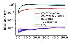
where is the neural network approximator to . Once trained, can be applied to to get the solution over . Repeating this process enables one to obtain approximation solutions in any finite time. However, this methodology may suffer from long-time instability. In fact, let us illustrate this using the Allen-Cahn equation (16) in one dimension. Figure 1 shows that the average errors of approximated solutions learned by DeepONets using both the single-shot loss (4) (labeled as DeepONet) and the time-integrated loss (5) (labeled as CONT DeepONet). Both errors accumulate rapidly as time increases, indicating the instability of the learned DeepONets in prediction of long-time solution. In contrast, our transfer-learning assisted DeepOnet dramatically reduces the error and stabilizes the prediction. For completeness, we also compare them with the Fourier Neural Operator(FNO) (Li et al. 2020), which is another state-of-the-art operator learning method.
2.2 DeepONet with transfer learning
The main idea of transfer learning is to train a neural network on a large data set and then partially freeze and apply it to a related but unseen task. Inspired by (Desai et al. 2021), we employ the transfer learning technique to successively correct the trained DeepONet at the prediction steps: we freeze the majority of the well-trained DeepONet and merely re-train the weights in the last hidden layer of the branch net by fitting the same physics-informed loss (4) defined by the underlying PDEs. To be more precise, by separating the parameters in the hidden layers and the parameter in the last layer of the branch net, we rewrite the branch net as
where are the outputs of the last hidden layer of the branch net and are the weights in the last layer. Inserting this into (2.1) gives
| (6) |
The architecture of the new operator network is illustrated in Figure 2.
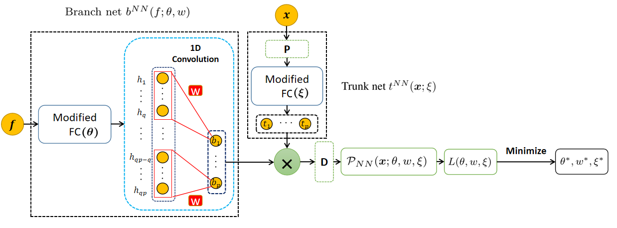
In the training step, the optimal parameters of the DeepONet (6) can be obtained by minimizing the empirical loss (4). Later in each prediction step, we freeze the value of and , but update by re-training the loss (4) with newly-predicted solution as the initial condition. Namely with the predicted solution at step , we seek defined by
| (7) |
Note that . The optimal sequence of weights defines a sequence of operator networks , which can be used to approximate the solution at by
It is interesting to note that the proposed method shares some similarities with the classical Galerkin approximation. In fact, the operator network (6) can be further rewritten as
Observe that playing the role of basis functions in Galerkin methods, and being the corresponding weight. However, unlike most Galerkin methods which often use handcraft bases, such as piecewise polynomials and trigonometric functions, here the bases are learned from the problem itself, and vary with the function they approximate. This seemly minor change reduces substantially the number of bases needed in the output space, as shown by extensive numerical tests in Section 4. To minimize (2.2), it amounts to solving a system of equations with unknowns, where is the total number of fixed sensors in the branch net. This is achieved by least square minimization. Since , the computational complexity of finding the least square solution is only . In practice, we further reduce the computational complexity by sub-sampling grid points out of in the transfer learning step.
3 Theoretical result
In this section, we analyze the long time stability of the learned operator . First let be a Banach space and assume that the original propagator (i.e., in (2)): is non-expansive such that
| (8) |
In the case that , assumption(8) follows from the dissipative assumption of ; see Appendix B.1 for more details. Let be a linear subspace, we also assume that
| (9) |
The theorem below shows that the long-time prediction error of the operator network can be bounded by the loss function.
Theorem 1.
Remark 1.
- 1.
-
2.
We comment on the assumptions made in Theorem 1. In practice, physics-informed loss (2.2) is trained so that condition (10) is fulfilled for some subspace space , e.g. . Assumption (9) holds for such a choice of when the evolution equation involves diffusion. Assumption (11) holds in particular when sine or cosine activation function is used in the operator network .
4 Numerical experiments
In this section, we demonstrate the effectiveness of transfer learning enhanced DeepONet and show its advantages over the vanilla DeepONet through several evolutionay PDEs, including reaction diffusion equation, Allen-Cahn and Cahn-Hilliard equations, Navier-Stokes equation and multiscale linear radiative transfer equation. The equations of consideration are equipped with either Dirichlet or periodic boundary conditions. In all the test problems, our goal is to predict the long time evolution of the equations obtained by successive actions of the propagators learned via DeepONets. More concretely, we first build the first-step neural operator approximation to the propagator by minimizing the physics-informed loss (4) with training initial data. The operator network is then gradually tuned to via updating the weights in the last-layer of its trunk nets. With the learned (and adjusted) operators , the solution of a PDE at time with an initial condition can then be obtained approximately by . We remark that the training data is constructed as a subset of a larger training set of size , which consists of pointwise evaluations of randomly sampled functions at physical locations (sensors). We refer to Appendix C.1 for detailed discussions on the data generating process and treatment of boundary conditions in various test problems. Choices of parameters for the operator networks and the training process are discussed in the end of Appendix C.1. In all the numerical results to follow, we quantify the performance of the proposed method by measuring the aggregated relative prediction error over a time horizon ; see the precise definition of the relative error in Appendix C.1. The codes used for the numerical experiments will be published on the website https://github.com/woodssss/TL-PI-DeepONet.
4.1 Reaction diffusion equation
Consider the reaction diffusion equation
| (15) |
where . In this example, we train DeepOnets and our transfer learning enhanced DeepONets using two different loss functions, with one based on the physics-informed loss within a single time-step (c.f. (4)), and the other based on the aggregated physics-informed loss (5) in the time window . We refer to the DeepONets trained using the latter loss as CONT DeepONets and reserve DeepONets for the one trained by the former loss. The numerical results of different DeepONets with varying training sample sizes are shown in Table 1. Our proposed method provides more accurate and more robust prediction of the solutions with little extra computational cost. In particular, the prediction error of vanilla DeepONets and CONT DeepONets increase dramatically as time increases from to , while transfer learning can significantly reduces the error and stabilizes the prediction in the long time. In addition, our method also substantially reduces the size of training data to achieve the same order of prediction accuracy. Note that, since trained only within a single time step, DeepONets take far less training time than the corresponding CONT DeepONets while maintain comparable accuracy. The similar trade-off of accuracy and training cost applies to other experiments. For this reason, in subsequent examples we will only report results on our proposed method and the vanilla DeepONet, and exclude the results from CONT DeepONets. Note also that the results obtained in Table 1 are for propagators defined by the backward Euler scheme. One can also consider propagators defined by higher order time-discretization schemes and their neural network approximation. We refer the numerical results obtained using the Crank-Nicolson method to Table 8 in Appendix C.2.
| Neural network | |||||
|---|---|---|---|---|---|
| CONT | 1000 | 43030 | 0.26 | 7.95e-2 | 4.17e-1 |
| DeepONet | 3000 | 79375 | 0.28 | 1.01e-2 | 4.15e-2 |
| 10000 | 83465 | 0.26 | 3.40e-3 | 1.34e-2 | |
| CONT | 1000 | 43030 | 0.93 | 5.38e-3 | 1.95e-3 |
| TL-DeepONet | 3000 | 79375 | 0.98 | 1.87e-3 | 6.88e-4 |
| 10000 | 83465 | 0.93 | 1.84e-3 | 4.87e-4 | |
| DeepONet | 1000 | 2575 | 5.02 | 2.75e-1 | 1.69e0 |
| 3000 | 4313 | 4.9 | 1.05e-1 | 1.60e0 | |
| 10000 | 5854 | 4.8 | 9.19e-2 | 1.87e0 | |
| TL-DeepONet | 1000 | 2575 | 9.86 | 1.03e-3 | 1.52e-3 |
| 3000 | 4313 | 7.1 | 8.34e-4 | 1.19e-3 | |
| 10000 | 5854 | 8.2 | 8.19e-4 | 9.05e-4 |
4.2 Allen-Cahn and Cahn-Hilliard equations
In the second example, we consider Allen-Cahn equation
| (16) |
and Cahn-Hilliard equation
| (17) |
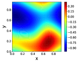
both equipped with periodic boundary conditions. They are prototype models for the motion of anti-phase boundaries in crystalline solids. The computational domain is with . We are interested in learning the propagator with and used it to predict the solutions for every . The results on Allen-Cahn equation are shown in Table 2 (1D) and Table 3 (2D). See also Figure 1 for a plot of evolving relative errors on 1D Allen-Cahn equation. Similar results for 1D Cahn-Hilliard equation are presented in Table 4 and Figure 3 compares the snapshots of predicted solutions to the 2D Cahn-Hilliard equation. In all the results, for a fixed , the relative errors increase as decreases because the transition layers of solutions are increasingly sharper and hence make the numerical resolution more challenging. Similar to the previous example, our proposed method provides more accurate prediction of solutions than the vanilla DeepONets among all the configurations of parameters. We note that the average trajectory prediction times of TL-DeepONets increase for about 3 times compared to those of the vanilla DeepONets while the prediction errors of the former decrease by at least two orders of magnitude.
| Neural network | =1e-3 | =5e-4 | =1e-4 | |
|---|---|---|---|---|
| DeepONet | 1000 | 1.13e0 | 1.33e0 | 1.29e0 |
| 3000 | 1.33e0 | 1.18e0 | 1.23e0 | |
| 10000 | 1.01e0 | 8.95e-1 | 1.43e0 | |
| TL-DeepONet | 1000 | 9.25e-4 | 9.64e-4 | 2.16e-2 |
| 3000 | 7.78e-4 | 8.83e-4 | 1.81e-2 | |
| 10000 | 5.81e-4 | 7.94e-4 | 1.16e-2 |
| Neural network | =4e-3 | =2e-3 | =1e-3 | |
|---|---|---|---|---|
| DeepONet | 1000 | 9.96e-1 | 1.01e0 | 1.02e0 |
| 10000 | 9.96e-1 | 1.00e0 | 1.00e0 | |
| TL-DeepONet | 1000 | 6.54e-3 | 8.43e-3 | 1.01e-2 |
| 10000 | 4.96e-3 | 6.46e-3 | 9.01e-3 |
| Neural network | =4e-6 | =2e-6 | =1e-6 | |
|---|---|---|---|---|
| DeepONet | 1000 | 9.43e-1 | 9.47e-1 | 9.44e-1 |
| 3000 | 9.54e-1 | 9.58e-1 | 9.39e-1 | |
| 10000 | 9.65e-1 | 9.58e-1 | 9.38e-1 | |
| TL-DeepONet | 1000 | 1.04e-2 | 1.36e-2 | 4.25e-2 |
| 3000 | 8.11e-3 | 9.04e-3 | 3.86e-2 | |
| 10000 | 2.29e-3 | 7.89e-3 | 3.03e-2 |
| Initical condition | t=4 | t=10 |
 |
 |
 |
| DeepONet | 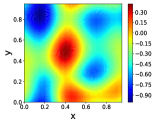 |
 |
| TL-DeepONet |  |
 |
4.3 Navier-Stokes equation
Consider the 2D Navier-Stokes equation in the vorticity form:
| (18) |
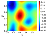
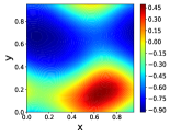
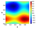
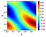
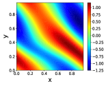
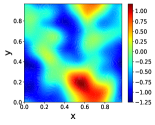
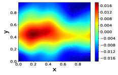
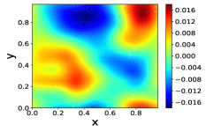
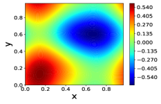
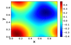
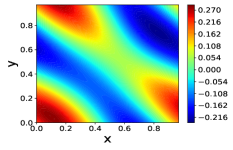
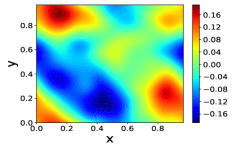
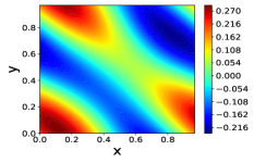
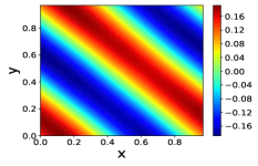
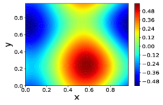
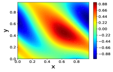
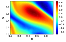
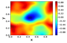
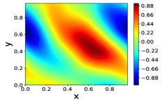
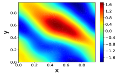
with periodic boundary condition and source . We would like to learn the propagator with and apply it to predict the solution . Table 5 shows the results with varying values of viscosity . Note that the prediction error increases as decreases. TL-DeepONets reduces the errors of DeepONets by two orders of magnitudes although the prediction time of the former increases for less than 4 times. Figure 4 shows the snapshots of solutions to (18) with at two different times.
| Neural network | =1e-1 | =1e-2 | =1e-3 | =1e-4 |
|---|---|---|---|---|
| DeepONet | 9.95e-1 | 1.02e0 | 9.96e-1 | 1.04e0 |
| TL-DeepONet | 1.41e-2 | 1.07e-2 | 3.35e-2 | 9.42e-2 |
| Initical condition | ||
 |
 |
 |
| DeepONet | 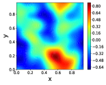 |
 |
| TL-DeepONet | 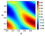 |
 |
4.4 Multiscale linear radiative transfer equation
Consider the linear multiscale radiative transfer equation:
| (19) |
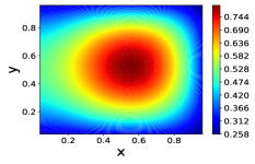
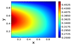
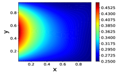
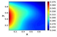
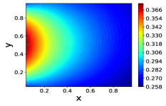
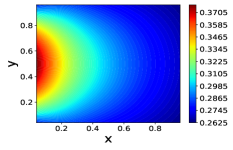
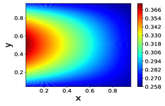
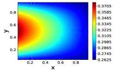
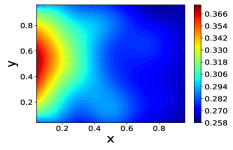
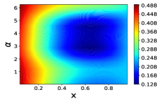
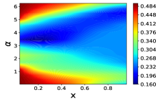
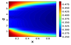
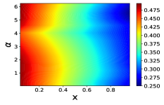
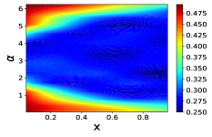
Here is the Knudsen number which is a dimensionless parameter that determines the physical regime of the equation, , and is the inflow part of the boundary. In this example, we aim to learn the propagator with and employ it to predict the solution for . We mainly consider (19) in one and two physical dimensions and refer to Appendix C.5 for a detailed discussion on the experiment set-up and the numerical method. Table 6 displays the results corresponding to different Knudsen numbers. The transfer learning enhanced DeepONets reduces the relative error by one or two orders of magnitude although increase the prediction time by around 4 times. Figure 9 and Figure 8 in Appendix C.5 show several snapshots of solutions to (19) with and respectively.
| RTE | Neural network | relative error | |
|---|---|---|---|
| 1D 1 | DeepONet | 4.6 | 3.06e-1 |
| TL-DeepONet | 22.5 | 1.52e-2 | |
| 1D 1e-4 | DeepONet | 5.1 | 3.74e-1 |
| TL-DeepONet | 21.9 | 5.52e-3 | |
| 2D 1 | DeepONet | 79.8 | 3.58e-1 |
| TL-DeepONet | 431.3 | 2.19e-2 | |
| 2D 1e-4 | DeepONet | 83.1 | 2.37e0 |
| TL-DeepONet | 379.3 | 8.93e-3 |
5 Conclusion
In this paper, we proposed a new physics-informed DeepONet based on transfer learning for learning evolutionary PDEs. This is achieved in two steps: first learn the propagators and then predict the solutions by successive actions of propagators on the initial condition. The experimental results demonstrated that the proposed method improves substantially upon the vanilla DeepONet in terms of long-time accuracy and stability while maintains low computational cost. The proposed method also reduced the training sample size needed to achieve the same order of prediction accuracy of the vanilla DeepONets.
Acknowledgement
L. Wang is partially supported by NSF grant DMS-1846854. Y. Lu thanks NSF for the support via the award DMS-2107934.
References
- Bhattacharya et al. (2020) Bhattacharya, K.; Hosseini, B.; Kovachki, N. B.; and Stuart, A. M. 2020. Model reduction and neural networks for parametric PDEs. arXiv preprint arXiv:2005.03180.
- Bozinovski and Fulgosi (1976) Bozinovski, S.; and Fulgosi, A. 1976. The influence of pattern similarity and transfer learning upon training of a base perceptron b2. In Proceedings of Symposium Informatica, volume 3, 121–126.
- Chakraborty et al. (2022) Chakraborty, A.; Anitescu, C.; Zhuang, X.; and Rabczuk, T. 2022. Domain adaptation based transfer learning approach for solving PDEs on complex geometries. Engineering with Computers, 1–20.
- Chen and Chen (1995) Chen, T.; and Chen, H. 1995. Universal approximation to nonlinear operators by neural networks with arbitrary activation functions and its application to dynamical systems. IEEE Transactions on Neural Networks, 6(4): 911–917.
- Desai et al. (2021) Desai, S.; Mattheakis, M.; Joy, H.; Protopapas, P.; and Roberts, S. 2021. One-Shot Transfer Learning of Physics-Informed Neural Networks. arXiv preprint arXiv:2110.11286.
- Do and Ng (2005) Do, C. B.; and Ng, A. Y. 2005. Transfer learning for text classification. Advances in neural information processing systems, 18.
- Goswami et al. (2019) Goswami, S.; Anitescu, C.; Chakraborty, S.; and Rabczuk, T. 2019. Transfer learning enhanced physics informed neural network for phase-field modeling of fracture. arXiv preprint arXiv:1907.02531.
- Goswami et al. (2022) Goswami, S.; Kontolati, K.; Shields, M. D.; and Karniadakis, G. E. 2022. Deep transfer learning for partial differential equations under conditional shift with DeepONet. arXiv preprint arXiv:2204.09810.
- Harris et al. (2020) Harris, C. R.; Millman, K. J.; van der Walt, S. J.; Gommers, R.; Virtanen, P.; Cournapeau, D.; Wieser, E.; Taylor, J.; Berg, S.; Smith, N. J.; Kern, R.; Picus, M.; Hoyer, S.; van Kerkwijk, M. H.; Brett, M.; Haldane, A.; del Río, J. F.; Wiebe, M.; Peterson, P.; Gérard-Marchant, P.; Sheppard, K.; Reddy, T.; Weckesser, W.; Abbasi, H.; Gohlke, C.; and Oliphant, T. E. 2020. Array programming with NumPy. Nature, 585(7825): 357–362.
- Jin, Cruz, and Gonçalves (2020) Jin, B.; Cruz, L.; and Gonçalves, N. 2020. Deep facial diagnosis: deep transfer learning from face recognition to facial diagnosis. IEEE Access, 8: 123649–123661.
- Kovachki et al. (2021) Kovachki, N.; Li, Z.; Liu, B.; Azizzadenesheli, K.; Bhattacharya, K.; Stuart, A.; and Anandkumar, A. 2021. Neural operator: Learning maps between function spaces. arXiv preprint arXiv:2108.08481.
- Li et al. (2020) Li, Z.; Kovachki, N.; Azizzadenesheli, K.; Liu, B.; Bhattacharya, K.; Stuart, A.; and Anandkumar, A. 2020. Fourier neural operator for parametric partial differential equations. arXiv preprint arXiv:2010.08895.
- Liu and Cai (2022) Liu, L.; and Cai, W. 2022. DeepPropNet–A Recursive Deep Propagator Neural Network for Learning Evolution PDE Operators. arXiv preprint arXiv:2202.13429.
- Lu, Jin, and Karniadakis (2019) Lu, L.; Jin, P.; and Karniadakis, G. E. 2019. Deeponet: Learning nonlinear operators for identifying differential equations based on the universal approximation theorem of operators. arXiv preprint arXiv:1910.03193.
- Lu et al. (2022) Lu, L.; Meng, X.; Cai, S.; Mao, Z.; Goswami, S.; Zhang, Z.; and Karniadakis, G. E. 2022. A comprehensive and fair comparison of two neural operators (with practical extensions) based on fair data. Computer Methods in Applied Mechanics and Engineering, 393: 114778.
- Lu, Wang, and Xu (2022) Lu, Y.; Wang, L.; and Xu, W. 2022. Solving multiscale steady radiative transfer equation using neural networks with uniform stability. Research in the Mathematical Sciences, 9(3): 1–29.
- Obiols-Sales et al. (2021) Obiols-Sales, O.; Vishnu, A.; Malaya, N. P.; and Chandramowlishwaran, A. 2021. SURFNet: Super-resolution of Turbulent Flows with Transfer Learning using Small Datasets. In 2021 30th International Conference on Parallel Architectures and Compilation Techniques (PACT), 331–344. IEEE.
- Raissi, Perdikaris, and Karniadakis (2019) Raissi, M.; Perdikaris, P.; and Karniadakis, G. E. 2019. Physics-informed neural networks: A deep learning framework for solving forward and inverse problems involving nonlinear partial differential equations. Journal of Computational physics, 378: 686–707.
- Ruder et al. (2019) Ruder, S.; Peters, M. E.; Swayamdipta, S.; and Wolf, T. 2019. Transfer learning in natural language processing. In Proceedings of the 2019 conference of the North American chapter of the association for computational linguistics: Tutorials, 15–18.
- Sirignano and Spiliopoulos (2018) Sirignano, J.; and Spiliopoulos, K. 2018. DGM: A deep learning algorithm for solving partial differential equations. Journal of computational physics, 375: 1339–1364.
- Song and Tartakovsky (2022) Song, D. H.; and Tartakovsky, D. M. 2022. TRANSFER LEARNING ON MULTIFIDELITY DATA. Journal of Machine Learning for Modeling and Computing, 3(1): 31–47.
- Virtanen et al. (2020) Virtanen, P.; Gommers, R.; Oliphant, T. E.; Haberland, M.; Reddy, T.; Cournapeau, D.; Burovski, E.; Peterson, P.; Weckesser, W.; Bright, J.; van der Walt, S. J.; Brett, M.; Wilson, J.; Millman, K. J.; Mayorov, N.; Nelson, A. R. J.; Jones, E.; Kern, R.; Larson, E.; Carey, C. J.; Polat, İ.; Feng, Y.; Moore, E. W.; VanderPlas, J.; Laxalde, D.; Perktold, J.; Cimrman, R.; Henriksen, I.; Quintero, E. A.; Harris, C. R.; Archibald, A. M.; Ribeiro, A. H.; Pedregosa, F.; van Mulbregt, P.; and SciPy 1.0 Contributors. 2020. SciPy 1.0: Fundamental Algorithms for Scientific Computing in Python. Nature Methods, 17: 261–272.
- Wang and Perdikaris (2021) Wang, S.; and Perdikaris, P. 2021. Long-time integration of parametric evolution equations with physics-informed deeponets. arXiv preprint arXiv:2106.05384.
- Wang, Wang, and Perdikaris (2021) Wang, S.; Wang, H.; and Perdikaris, P. 2021. Learning the solution operator of parametric partial differential equations with physics-informed DeepONets. Science advances, 7(40): eabi8605.
- Yin et al. (2019) Yin, X.; Yu, X.; Sohn, K.; Liu, X.; and Chandraker, M. 2019. Feature transfer learning for face recognition with under-represented data. In Proceedings of the IEEE/CVF conference on computer vision and pattern recognition, 5704–5713.
- Yu et al. (2018) Yu, B.; et al. 2018. The deep Ritz method: a deep learning-based numerical algorithm for solving variational problems. Communications in Mathematics and Statistics, 6(1): 1–12.
- Zang et al. (2020) Zang, Y.; Bao, G.; Ye, X.; and Zhou, H. 2020. Weak adversarial networks for high-dimensional partial differential equations. Journal of Computational Physics, 411: 109409.
A Table of notations
A table of notations is given in Table 7.
| Notation | Meaning |
|---|---|
| Target propagator | |
| Neural network approximator | |
| The Banach space of input functions | |
| The interior sensors | |
| The boundary sensors | |
| Randomly sampled functions used for training | |
| Neural network parameters | |
| The branch net of DeepONet | |
| The output functions defined by the last | |
| hidden layer in the branch net | |
| The trunk net of DeepONet | |
| Weights in the last layer of the branch net | |
| Number of sensors | |
| Number of grid points | |
| in transfer learning step | |
| Number of training sample pairs | |
| Number of output features | |
| Number of tunable weights at the last hidden layer of the branch net |
B Theoretical analysis
B.1 Validation of assumption (8)
Here we will give a simple justification for the assumption (8). Consider the norm as an example:
then (8) is fulfilled if the underlying dynamics is stable under this norm:
where is the solution to (1). Indeed, multiplying (1) by and integrating in , we have
Then for the semi-discrete in time version
multiplying it by and integrating in , it becomes
which readily leads to
B.2 Proof of Theorem 1
C Experiment details
In this section, we provide the details on the numerical experiments of Section 4.
C.1 Data generation and configuration of training
Data generation
For all numerical experiments, we use uniform mesh with grid points for discretization of the spatial domain , and Gaussian quadrature points for discretizing the velocity variable in the radiative transfer equation only. We generate initial conditions for training and functions for testing. The training set consists of functions that sampled from a centered Gaussian random field as well as forward passes of those functions through up to times actions of the propagator. This gives training functions. The random functions may be post-processed so that they satisfy the boundary condition of the PDE. Details on the post-processing methods can be found in the subsequent sections. The final training data of size is constructed as a subset of a larger training set of size , which consists of pointwise evaluations of randomly sampled functions at physical locations (sensors). Unless otherwise specified, we set , in 1D test problems and , in 2D test problems. Here a training set of size may only use 50 functions evaluating at 20 grid points in the domain.
Two error measures.
To quantify the performance of our neural nets, we measure two relative errors of neural operator approaches. The first is the relative error at a single time-step :
| (22) |
and the second is the relative error over a long time horizon (or equivalently multiple time steps)
| (23) |
Neural networks and training parameters
In 1D examples, we use the modified fully connected architecture with depth of 5 layers and width of 100 neurons for both branch and trunk nets, and the design of the optional layers and in Figure 2 will be detailed in each of the following examples. The batch size is chosen to be 100 with ADAM optimizer, where the initial learning rate and a 0.95 decay rate in every 5000 steps. Same architecture is used in 2D examples except that a depth of 6 layers is used. In the transfer learning step, to solve the optimization problem (2.2), we use the lstsq function (with rcond=1e-6) from Numpy(Harris et al. 2020) for linear operators and the leastsq function in Scipy(Virtanen et al. 2020) (using default setting with 1e-5, 1e-5) for nonlinear operators. All of the neural networks are trained on a single K40m GPU, and the prediction step is computed on a AMD Ryzen 7 3700x Processor.
C.2 Further details on reaction diffusion equation
To generate initial conditions that satisfy zero boundary condition, i.e., we first sample with
| (24) |
and then let . Likewise, to enforce the same boundary condition for the output of the neural net, i.e., , we employ an additional layer in Figure 2 that multiplies the output of trunk nets by .
Crank-Nicolson scheme for reaction diffusion equation
To demonstrate the improvement on the efficiency of using the higher order in time scheme at the transfer learning step, we apply Crank-Nicolson scheme for the nonlinear reaction diffusion equation. As displayed in Table 8, the second order scheme with reduces the prediction time compared with first order scheme with by a factor of .
| Neural network | Relative error | ||
|---|---|---|---|
| TL-DeepONet | 7.1 | 1.78e-3 | |
| TL-DeepONet 2nd | 4.53 | 4.91e-4 | |
| 2.36 | 2.63e-3 | ||
| 1.24 | 9.53e-3 |
Implementation details on Table 1 and Table 8
Consider 1D nonlinear reaction diffusion equation (15) with . We use test functions drawn from the Gaussian process defined above with the length scale in (24) and we use uniform spatial grids for spatial discretization. The loss functions of CONT DeepONet and CONT TL-DeepONet (c.f. (5)) are calculated using 20 uniform temporal steps on . For DeepONet and TL-DeepONet, we set the maximum iteration number and adopt the stopping criterion that the empirical loss is below 1e-6. For CONT DeepONet and CONT TL-DeepONet, we set maximum iteration number and use stopping criterion that the empirical loss is below 1e-6. We use features for all four operator networks. In the transfer learning steps of CONT TL-DeepONet, we subsample grid points and update weights defined in (6). In the transfer learning steps of TL-DeepONet, we set and instead. Additionally, we fix in Table 1 and in Table 8.
C.3 Further details on Allen-Cahn and Cahn-Hilliard equation
In all three examples, we consider periodic boundary conditions. To this end, the initial condition is generated from , where the covariance kernel has the desired periodicity. In particular, the kernel in one dimension reads:
| (25) |
and in two dimension takes the form:
| (26) |
To enforce the periodic boundary condition to the output of the trunk net, we employ an additional layer (see Figure 2) in the truck net, which upsizes to .This way, the input of the trunk net already has the desired periodicity and will be maintained throughout. Analogously, an additional layer , which plays the role of upsizing to , is leveraged in the trunk net in 2D case.
Implementation details on Figure 1 and Table 2, 3
Consider Allen-Cahn equation (16) with . In 1D case, we use test functions drawn from the Gaussian process defined above with the length scale in (25) and use uniform spatial grids for spatial discretization. For DeepONet and TL-DeepONet, we let time step size , set the maximum iteration number and adopt the stopping criterion that the empirical loss is below 1e-6. For CONT DeepONet and CONT TL-DeepONet, we use additional 20 uniform grids on time span , set maximum iteration number and use stopping criterion that the empirical loss is below 1e-6. We use features for all four operator networks. In the transfer learning steps of CONT TL-DeepONet, we subsample grid points and update weights defined in (6). In the transfer learning steps of TL-DeepONet, we set and instead. In 2D case, we use test functions drawn from the Gaussian process defined above with the length scale in (26). We use for time step size and uniform spatial grids for spatial discretization. We set the maximum iteration number , adopt the stopping criterion that the empirical loss is below 1e-6 and use number of feature . In the transfer learning step, we subsample and update weights defined in (6). Additionally, we fix and in Figure 1. For FNO in Figure 1, we choose the time step size , prepare 50 Input & Ouput function pairs, set the maximum iteration number and adopt the stopping criterion that the empirical loss is below 1e-6.
Implementation details on Table 4 and Figure 3
Consider Cahn-Hilliard equation (17) with . In 1D case, we use test functions drawn from the Gaussian process defined above with the length scale in (25). We use for time step size and uniform spatial grids for spatial discretization. We set the maximum iteration number , adopt the stopping criterion that the empirical loss is below 1e-6 and use number of feature . In the transfer learning step, we subsample and update weights defined in (6). In 2D case, we use test functions drawn from the Gaussian process defined above with the length scale in (26). We use for time step size and uniform spatial grids for spatial discretization. We set the maximum iteration number , adopt the stopping criterion that the empirical loss is below 1e-6 and use number of feature . In the transfer learning step, we subsample and update weights defined in (6). Additionally, we fix 2e-6 and in Figure 3.
C.4 Further details on Navier-Stokes equation
The data generation of Navier-Stokes equation and the design of optional layer in Figure 2 are exactly same as the one to Allen-Cahn and Cahn-Hilliard equation in Section C.3.
Calculation of Navie-Stokes equation
By introducing the stream function , the velocity field and the vorticity can be found from and . Therefore, we rewirte the equation (18) as
| (27) |
and use the following semi-discretization scheme in the computation of the numerical solutions:
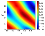
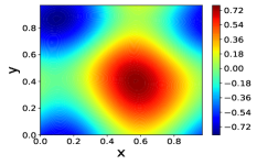
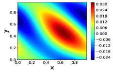
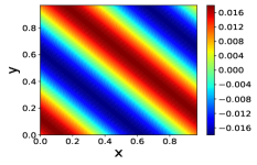
Supplementary examples of Navier-Stokes equation
| Initical condition | |||
 |
 |
 |
 |
| DeepONet | 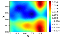 |
 |
 |
| TL-DeepONet |  |
 |
 |
| Initical condition | |||
 |
 |
 |
 |
| DeepONet | 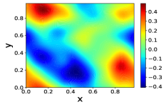 |
 |
 |
| TL-DeepONet | 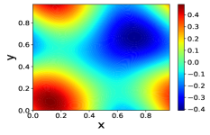 |
 |
 |
| Initical condition | |||
 |
 |
 |
 |
| DeepONet | 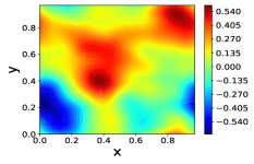 |
 |
 |
| TL-DeepONet | 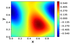 |
 |
 |
Implementation details on Table 5 and Figures 5,6,4, 7
Consider 2D Navier-Stokes equation (18). We use test functions drawn from the Gaussian process defined above with the length scale in (26). We use for time step size and uniform spatial grids for spatial discretization. We set the maximum iteration number , adopt the stopping criterion that the empirical loss is below 1e-6 and use number of feature . In the transfer learning step, we subsample and update weights defined in (6).
C.5 Details on Multiscale linear radiative transfer equation
Computation of multiscale radiative transfer equation
Following (Lu, Wang, and Xu 2022), instead of discretizing the original radiative transfer equation (19), we consider a new system of equations based on its micro-macro decomposition. More concretely, let . We consider
| (28) |
It was shown in (Lu, Wang, and Xu 2022) that the PINN loss based on (19) suffers from the instability issue when the small Knudsen number is small while the PINN loss based on the system (28) above is uniformly stable with respect to the small Knudsen number in the sense that the -error of the neural network solution is uniformly controlled by the loss. We consider (19) and its equivalent system (28) in one and two dimensions. To enforce the inflow boundary condition
we first parameterize as follows:
| (29) |
where , and are determined according to the specific boundary conditions in each example, whilst and are to-be approximated by the neural nets. In other words, instead of using two neural nets to approximate and , we approximate and , and recover and via
and
1D Example
Here the computational domain is and the inflow boundary condition takes the form:
Then in (29) we use
where is the ReLU function. In the same vein, we generate the initial data by first sampling with
| (30) |
and then selecting those that are strictly positive to construct
2D Example
Consider the spatial domain as , and velocity variable is with . The inflow boundary condition reads:
Then to guarantee that in (29) satisfies this condition, we choose
Similarly, the initial conditions are generated by first sampling with
| (31) |
and then retaining only the positive samples to construct via:
Supplementary examples of radiative transfer equation
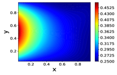
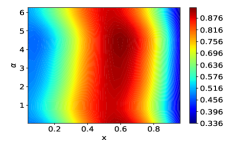
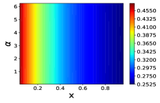
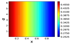
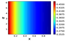
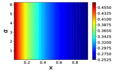
Here we provide the snapshots of solution to (19) in 2D with and in Figure 8 and Figure 9, respectively.
| Initical condition | |||
|---|---|---|---|
 |
 |
 |
 |
| DeepONet | 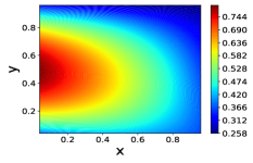 |
 |
 |
| TL-DeepONet | 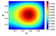 |
 |
 |
| Initical condition | |||
|---|---|---|---|
 |
 |
 |
 |
| DeepONet | 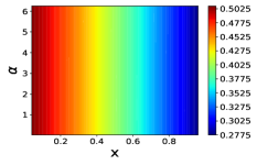 |
 |
 |
| TL-DeepONet | 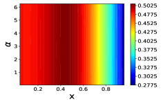 |
 |
 |
| Initical condition | |||
|---|---|---|---|
 |
 |
 |
 |
| DeepONet |  |
 |
 |
| TL-DeepONet | 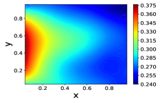 |
 |
 |
| Initical condition | |||
|---|---|---|---|
 |
 |
 |
 |
| DeepONet |  |
 |
 |
| TL-DeepONet |  |
 |
 |
Implementation details on Table 6 and Figures 8,9
Consider multiscale radiative transfer equation (19). In 1D case, we use test functions drawn from the Gaussian process defined above with the length scale in (30). We use for time step size, uniform spatial grids for spatial discretization and Gaussian quadrature points for velocity discretization. We set the maximum iteration number , adopt the stopping criterion that the empirical loss is below 1e-6 and use number of feature . In the transfer learning step, we update weights defined in (6). In 2D case, we use test functions drawn from the Gaussian process defined above with the length scale in (31). We use for time step size, uniform spatial grids for spatial discretization and Gaussian quadrature points for velocity discretization. We set the maximum iteration number , adopt the stopping criterion that the empirical loss is below 1e-6 and use number of feature . In the transfer learning step, we update weights defined in (6).