Using X-ray continuum-fitting to estimate the spin of MAXI J1305-704

Abstract

MAXI J1305-704 is a transient X-ray binary with a black hole primary. It was discovered on April 9, 2012, during its only known outburst. MAXI J1305-704 is also a high inclination low-mass X-ray binary with prominent dip features in its light curves, so we check the full catalog of 92 Swift/XRT continuous observations of MAXI J1305-704, focusing only on the stable spectra. We select 13 “gold" spectra for which the root mean square RMS <0.075 and the coronal scattered fraction $f_{\mathrm{sc}}\lesssim 25\%$. These “gold" data are optimal thermal-state observations for continuum-fitting modeling, in which the disk extends to the innermost-stable circular orbit and is geometrically thin. The black hole spin was unknown for this object before. By utilizing the X-ray continuum fitting method with the relativistic thin disk model kerrbb2 and supplying the known dynamical binary system parameters, we find MAXI J1305-704 has a moderate spin ($a_{*}=0.87_{-0.13}^{+0.07}$) at a 68.3% confidence level. This is the first determination of MAXI J1305-704’s spin.

1 Introduction

The incredible ‘no-hair theorem’ reveals that an astrophysical BH is completely describable by just two quantities: mass and spin. Spin, which can be described by a dimensionless parameter $a_{*}=cJ/GM^{2}$. Generally, there are two mainstream spectroscopic approaches to constrain the spin of the black hole: the X-ray reflection fitting method (Fabian et al. 1989) and the X-ray continuum-fitting (CF) method (Zhang et al. 1997). The reflection method has been applied to numerous black holes residing in X-ray binary (BHXRB) systems, e.g., XTE J1550-564 (Steiner et al. 2011), GRS 1915+105 (Miller et al. 2013), GS 1354-645 (El-Batal et al. 2016), MAXI J1535-571 (Xu et al. 2018), XTE J1752-223 (García et al. 2018), MAXI J1836-194 (Morningstar & Miller 2014; Dong et al. 2020), EXO 1846-031(Draghis et al. 2020), and CF has been widely applied, e.g., GRS 1915+105 (McClintock et al. 2006; Middleton et al. 2006), M33 X-7 (Liu et al. 2008), A 0620-00 (Gou et al. 2010), XTE J1550-564 (Steiner et al. 2011), Cyg X-1 (Gou et al. 2014), GS 1124-683 (Morningstar et al. 2014; Chen et al. 2016).

In the CF method, the inner disk radius ($R_{\rm in}$) is measured by fitting the thermal continuum emission of the accretion disk, which is based on the assumptions of the classical relativistic thin disk model (Novikov & Thorne 1973). By assuming that the inner radius of the accretion disk extends to the innermost stable circular orbit (ISCO), we can estimate the spin using the unique mapping between ISCO and spin discovered in Bardeen et al. (1972). The CF approach generally requires independent knowledge of system properties, black hole mass ($M$), the source distance ($D$), and accretion disk inclination ($i$, often requiring an assumption that the spin of a black hole is aligned with the orbital angular momentum). The X-ray reflection fitting method also measures the inner disk radius by reprocessing coronal emission in the surface of the disk, especially the Fe K$\alpha$ emission complex. Notably, CF is most reliable in soft/thermal states in which coronal emission is weakest whereas reflection methods are most useful in hard or intermediate states where the coronal emission is strong or dominant. In reflection modeling, the inclination may be fitted in addition to the spin. The CF method is typically used for stellar-mass black holes, whereas the reflection fitting method is widely used for both stellar-mass and supermassive black holes. Apart from the mutual reliance on the relationship between the inner disk radius and the ISCO, both methods are independent and can be used to cross-check each other. We use the CF method to estimate the spin of MAXI J1305-704 in this paper.

Of the approximately 70 black holes and black hole candidate systems detected so far, only five systems are wind-fed and persistent (Cygnus X-1, LMC X-1, M33 X-7, NGC 300 X-1, and IC 10 X-1), while the rest are transient. MAXI J1305-704 is a member of the latter group. It is a Galactic (RA=196.7^∘, Dec=-70.5^∘) black hole X-ray binary with a peak flux of 30 mCrab (1 Crab = $2.4\times 10^{-8}$ $\rm ergs^{-1}cm^{-2}$ for 2.0-10.0 keV) in the 2.0-4.0 keV band (Sato et al. 2012). MAXI J1305-704 was first noticed by the Monitor of an All-sky X-ray Image/Gas Slit Camera (MAXI/GSC) (Sato et al. 2012) on 2012 April 9 at 11:24:23 UT. Multiple wavelength analyses indicated that the source is most likely a BHXRB (Greiner et al. 2012; Kennea et al. 2012a; Suwa et al. 2012; Charles et al. 2012; Morihana et al. 2013). It exhibited canonical hard, intermediate, and soft states during the outburst (Suwa et al. 2012; Morihana et al. 2013). A ground-based dynamical study performed in quiescence later confirmed that MAXI J1305-704 is a black hole with the mass of $M_{\rm BH}=8.9_{-1.0}^{+1.6}M_{\odot}$, a companion mass of $M_{\mathrm{opt}}=0.43\pm 0.16M_{\odot}$, at a distance of $D=7.5_{-1.4}^{+1.8}\mathrm{kpc}$, and a high inclination of $i={72_{-8}^{+5}}^{\circ}$ (uncertainties are 1 $\sigma$; Mata Sánchez et al. 2021). From these data, we are able to apply CF and measure its spin. Previous studies have shown that MAXI J1305-704 is an anomalous source, showing a very high disk temperature ($\sim$1.0 keV) in the soft state, even while at extremely low luminosity ($\sim$0.02 $L_{\mathrm{Edd}}$) (Shidatsu et al. 2013; Morihana et al. 2013). In general, black holes with such high disk temperatures usually have relatively large luminosity.

Using the Mata Sánchez et al. (2021) dynamical results, we apply the relativistic thin-disk model kerrbb2 (McClintock et al. 2006; which merges two different disk models, kerrbb (Li et al. 2005) and bhspec (Davis et al. 2005)) with CF approach to fit an optimal selection of 13 “gold" spectra (13 selected spectra of Swift/XRT in the soft state during its 2012 outburst) so as to further constrain its spin. This is because, in the soft state, the inner radius of the accretion disk has extended to ISCO, and at sufficiently low luminosities the accretion disk conforms to a standard thin disk structure.

The structure of the paper is as follows. We present data selection and reduction in Section 2. Section 3 delves deeply into the spectral analysis and results. Sections 4 and 5 present the discussions and conclusion respectively.

2 DATA SELECTION AND REDUCTION

From MAXI/GSC’s thirteen years of coverage, MAXI J1305-704 exhibited only one significant outburst in 2012 as shown in Figure 1, nor was it detected by predecessor X-ray sky monitors (e.g., Swift/BAT or RXTE/ASM). The corresponding hardness-intensity diagram (HID) in Figure 1 exhibits a non-standard shape, distinct from the usual “q"-like profile typical of major outbursts by BHXRBs. During this outburst in 2012, Swift/XRT (Burrows et al. 2005) had two observing programs (00032339XXX and 00032461XXX), totaling 65 observations containing 92 continuous data segments. Consistent with its high orbital inclination (and similar to other high-inclination BHXRBs), MAXI J1305-704 exhibited obvious dip characteristics in its light-curves (e.g., Kennea et al. 2012b; Kennea et al. 2012c; Shidatsu et al. 2013; Miller et al. 2014). Regarding the 65 observations by Swift/XRT, we used the FTOOLS command ftselect to divide them by Good Time Interval (GTI), into 92 spectra and light curves, which are summarized in Table 1. Figure 2 shows the hardness evolution over time. Figure 3 depicts three types of features of the light curve for illustration. In general, the spectra used to measure the spin should have no dips, flares, or other sizeable variations. Each light curve is screened by eye to exclude data sets with dips or presenting high variability. “Dip" light curves (Figure 3) display one or more sharply-shaped deficits in count rate, whereas “variable" light curves (Figure 3) show significant variations that are inconsistent with a stable and fixed count rate. To ensure robustness, spectra are required to have at least 8000 counts. We also screen for spectra whose emission is dominated by the accretion disk (McClintock et al. 2006) since the CF technique relies upon the signal of the thermal disk component, and also presumes that the inner radius of the disk reaches the ISCO, which is most firmly grounded for soft disk-dominated states (e.g., Tanaka & Lewin 1995; Kubota & Done 2003; Steiner et al. 2010). This also eliminates the possibility of contamination by a strong Compton component. We adopt an upper limit on the root mean square (RMS) variability (RMS < 0.075, Remillard & McClintock 2006) and the relative strength of the non-thermal emission ($f_{\mathrm{sc}}\lesssim 25\%$, where $f_{\mathrm{sc}}$ is the relative strength of the Comptonization model simpl in XSPEC. See Steiner et al. 2009a; Steiner et al. 2009b). More details are given in Section 3.1.

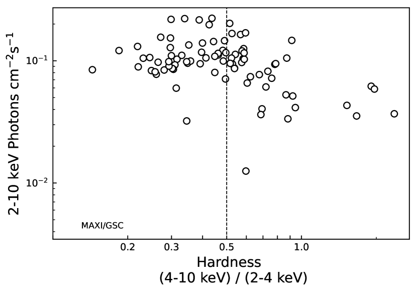
Figure 1: a) The light curve of the MAXI J1305-704 outburst was observed by MAXI/GSC in 2012. The colored arrows mark the dates of SP1 through SP13. b) The HID of MAXI J1305-704 is based on MAXI/GSC measurements. It corresponds to the outburst from MJD=56022 to MJD=56120 in Figure 1. The MAXI/GSC hardness is expressed as the ratio of counts measured at 4.0-10.0 keV to counts detected at 2.0-4.0 keV. A dashed line at a hardness value of 0.5 is included as a visual reference.

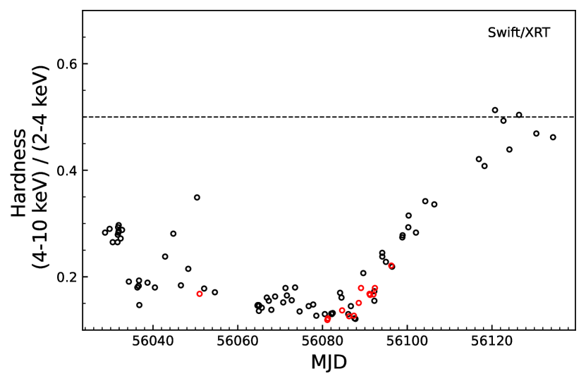
Figure 2: The hardness over time for 92 spectra of Swift/XRT, using 4.0-10.0 keV/2.0-4.0 keV rates, but with different amplitude than the MAXI/GSC values in Figure 1 owing to differences in the instruments. SP1-SP13 are marked in red. A dashed line at a hardness value of 0.5 is included as a visual reference.

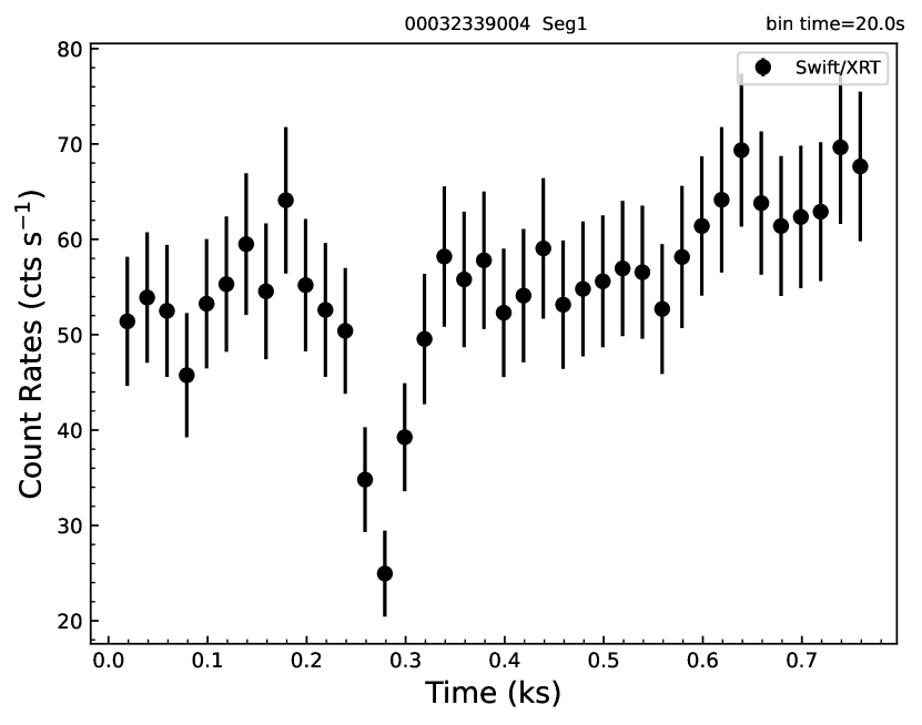
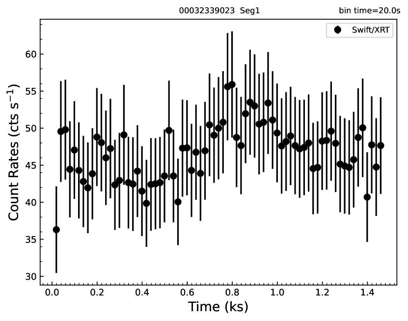
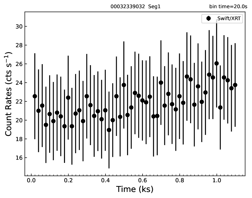
Figure 3: a) N9 (ObsID: 00032339004 Seg1), an observation of Swift/XRT, where the net light curve generated at 0.3-10.0 keV displays a noticeable dip. b) N43 (ObsID: 00032339023 Seg1), an observation of Swift/XRT, where the net light curve generated at 0.3-10.0 keV shows a significant variation. c) N69 (ObsID: 00032339032 Seg1), an observation of Swift/XRT, where the stable net light curve generated at 0.3-10.0 keV.

Figure 4: The PSD plot (with Leahy normalization while having subtracted off the Poisson noise) for N48 (SP2) (ObsId:00032461008 Seg1), which is representative of the other thermal data. The RMS value is $0.011\pm 0.007$, and the frequency range is from 0.017 to 139 Hz.

Table 1: MAXI J1305-704 Swift/XRT observation overview

Number	ObsID	Seg.	MJD	Start time	Exposure	Count Rates	Phase	RMS	LC type	$f_{\rm sc}$
					(s)	(cts $\rm s^{-1}$)
N1	00032339001	Seg1	56028	2012-04-11 16:08:46.801	997	44.27	0.000-0.029	0.137 $\pm$ 0.005	variable	-
N2	00032339002	Seg1	56029	2012-04-12 17:54:32.401	1282	46.67	0.718-0.755	0.084 $\pm$ 0.004	dips	-
N3	00032339003	Seg1	56030	2012-04-13 11:30:40.601	858	55.14	0.574-0.600	0.094 $\pm$ 0.005	variable	-
N4	00032339006	Seg1	56031	2012-04-14 14:42:48.001	2418	51.83	0.444-0.515	0.110 $\pm$ 0.003	dips	-
N5	00032339006	Seg2	56031	2012-04-14 16:18:03.601	2474	59.60	0.611-0.684	0.086 $\pm$ 0.003	dips	-
N6	00032339006	Seg3	56031	2012-04-14 17:54:44.801	2443	29.64	0.781-0.853	0.146 $\pm$ 0.004	dips	-
N7	00032339006	Seg4	56031	2012-04-14 19:29:49.201	2513	37.40	0.948-0.023	0.071 $\pm$ 0.003	dips	-
N8	00032339006	Seg5	56031	2012-04-14 21:23:23.201	129	56.40	0.148-0.152	0.035 $\pm$ 0.012	stable	-
N9	00032339004	Seg1	56031	2012-04-14 21:26:11.801	763	55.51	0.153-0.175	0.128 $\pm$ 0.005	dips	-
N10	00032339005	Seg1	56032	2012-04-15 08:23:37.001	683	53.12	0.309-0.330	0.088 $\pm$ 0.005	stable	-
N11	00032339005	Seg2	56032	2012-04-15 16:23:24.801	693	61.06	0.152-0.173	0.066 $\pm$ 0.005	variable	-
N12	00032339007	Seg1	56034	2012-04-17 06:58:08.401	1068	36.31	0.222-0.253	0.169 $\pm$ 0.005	dips	-
N13	00032339008	Seg1	56036	2012-04-19 07:09:15.201	943	36.17	0.305-0.332	0.088 $\pm$ 0.005	dips	-
N14	00032339009	Seg1	56036	2012-04-19 13:19:54.201	2459	20.50	0.956-0.028	0.166 $\pm$ 0.004	dips	-
N15	00032339009	Seg2	56036	2012-04-19 14:56:45.401	2419	30.42	0.127-0.198	0.125 $\pm$ 0.004	dips	-
N16	00032339009	Seg3	56036	2012-04-19 16:30:53.601	2543	33.27	0.292-0.367	0.165 $\pm$ 0.003	dips	-
N17	00032339009	Seg4	56036	2012-04-19 18:18:42.201	87	41.50	0.482-0.485	< 0.020	stable	-
N18	00032339009	Seg5	56038	2012-04-21 16:46:57.201	958	45.73	0.384-0.412	0.076 $\pm$ 0.005	variable	-
N19	00032339010	Seg1	56040	2012-04-23 10:34:56.201	470	43.38	0.793-0.807	0.155 $\pm$ 0.007	dips	-
N20	00032339011	Seg1	56042	2012-04-25 20:24:11.601	943	24.74	0.892-0.920	0.115 $\pm$ 0.007	dips	-
N21	00032339012	Seg1	56044	2012-04-27 18:53:20.201	818	25.03	0.796-0.820	0.177 $\pm$ 0.007	dips	-
N22	00032339013	Seg1	56046	2012-04-29 13:51:04.601	1013	50.78	0.328-0.357	0.070 $\pm$ 0.004	variable	-
N23	00032339014	Seg1	56048	2012-05-01 07:31:04.801	893	29.63	0.723-0.749	< 0.006	variable	-
N24	00032339015	Seg1	56050	2012-05-03 09:17:51.601	667	5.31	0.974-0.994	0.378 $\pm$ 0.017	variable	-
N25	00032339015	Seg2	56050	2012-05-03 23:39:55.001	723	43.76	0.489-0.511	0.062 $\pm$ 0.006	stable	0.098 $\pm$ 0.012
N26	00032339016	Seg1	56052	2012-05-05 01:26:51.201	967	17.08	0.209-0.237	0.163 $\pm$ 0.008	dips	-
N27	00032339017	Seg1	56054	2012-05-07 14:21:16.601	997	35.85	0.634-0.663	0.057 $\pm$ 0.005	variable	-
N28	00032461001	Seg1	56064	2012-05-17 15:41:23.001	696	32.83	0.091-0.112	0.088 $\pm$ 0.007	variable	-
N29	00032461001	Seg2	56064	2012-05-17 17:17:23.001	753	35.77	0.260-0.282	0.123 $\pm$ 0.006	variable	-
N30	00032339018	Seg1	56064	2012-05-17 22:02:22.801	457	30.29	0.761-0.775	0.086 $\pm$ 0.009	variable	-
N31	00032339018	Seg2	56064	2012-05-17 23:36:47.801	488	32.77	0.927-0.941	0.083 $\pm$ 0.008	variable	-
N32	00032461002	Seg1	56065	2012-05-18 01:12:16.601	463	31.85	0.095-0.109	0.113 $\pm$ 0.009	variable	-
N33	00032461002	Seg2	56065	2012-05-18 15:56:06.201	174	24.80	0.649-0.654	0.098 $\pm$ 0.018	variable	-
N34	00032339019	Seg1	56066	2012-05-19 20:24:52.801	1023	34.79	0.653-0.683	0.132 $\pm$ 0.005	variable	-
N35	00032461003	Seg1	56067	2012-05-20 07:45:17.001	343	35.13	0.849-0.860	< 0.010	variable	-
N36	00032461003	Seg2	56067	2012-05-20 22:11:19.001	518	38.51	0.372-0.387	0.100 $\pm$ 0.007	variable	-
N37	00032461004	Seg1	56068	2012-05-21 19:20:13.001	164	43.75	0.602-0.607	0.066 $\pm$ 0.014	variable	-
N38	00032339021	Seg1	56070	2012-05-23 17:32:14.601	984	19.07	0.476-0.505	0.151 $\pm$ 0.007	stable	-
N39	00032461005	Seg1	56071	2012-05-24 06:12:02.601	717	47.56	0.812-0.833	0.084 $\pm$ 0.005	variable	-
N40	00032461005	Seg2	56071	2012-05-24 14:10:32.001	443	44.02	0.653-0.666	<0.007	variable	-
N41	00032339022	Seg1	56072	2012-05-25 17:33:18.601	1417	47.67	0.541-0.583	0.073 $\pm$ 0.004	variable	-
N42	00032461006	Seg1	56073	2012-05-26 12:38:41.801	1452	50.33	0.555-0.597	<0.004	variable	-
N43	00032339023	Seg1	56074	2012-05-27 14:15:20.601	1477	46.89	0.256-0.300	< 0.004	variable	-
N44	00032339024	Seg1	56076	2012-05-29 17:35:42.401	1452	48.56	0.672-0.714	0.080 $\pm$ 0.004	variable	-
N45	00032461007	Seg1	56077	2012-05-30 19:15:30.801	1407	27.53	0.379-0.420	0.077 $\pm$ 0.005	variable	-
N46	00032339025	Seg1	56078	2012-05-31 12:55:51.401	966	20.10	0.243-0.272	0.136 $\pm$ 0.007	stable	-
N47	00032339026	Seg1	56080	2012-06-02 13:06:25.401	933	29.45	0.325-0.352	0.098 $\pm$ 0.006	variable	-
N48	00032461008	Seg1	56081	2012-06-03 03:20:06.801	532	42.53	0.826-0.842	0.011 $\pm$ 0.007	stable	0.051 $\pm$ 0.010
N49	00032461008	Seg2	56081	2012-06-03 06:32:06.201	473	44.48	0.163-0.177	< 0.007	stable	0.072 $\pm$ 0.011
N50	00032461009	Seg1	56082	2012-06-04 01:47:07.201	712	30.20	0.194-0.216	< 0.007	dips	-
N51	00032339027	Seg1	56082	2012-06-04 05:06:45.401	1085	30.65	0.545-0.577	0.098 $\pm$ 0.006	variable	-
N52	00032461009	Seg2	56082	2012-06-04 09:57:14.401	643	34.63	0.056-0.075	< 0.007	variable	-
N53	00032461010	Seg1	56084	2012-06-06 03:27:44.601	1334	20.09	0.434-0.474	0.091 $\pm$ 0.006	variable	-
N54	00032461010	Seg2	56084	2012-06-06 11:28:44.401	1153	49.86	0.280-0.314	< 0.004	dips	-
N55	00032339028	Seg1	56084	2012-06-06 15:01:15.201	1003	46.42	0.653-0.683	0.023 $\pm$ 0.005	stable	0.076 $\pm$ 0.007
N56	00032461011	Seg1	56086	2012-06-08 01:58:19.201	1001	36.23	0.340-0.370	0.062 $\pm$ 0.005	variable	-
N57	00032461011	Seg2	56086	2012-06-08 06:45:19.201	938	41.04	0.845-0.872	< 0.005	stable	0.064 $\pm$ 0.007
N58	00032339029	Seg1	56086	2012-06-08 16:35:17.801	997	42.98	0.882-0.911	0.036 $\pm$ 0.005	variable	-
N59	00032461012	Seg1	56087	2012-06-09 10:00:19.201	820	44.80	0.719-0.744	< 0.005	stable	0.059 $\pm$ 0.007
N60	00032461012	Seg2	56087	2012-06-09 13:15:19.201	640	46.96	0.062-0.082	< 0.006	variable	-
N61	00032461012	Seg3	56087	2012-06-09 18:22:07.401	768	45.68	0.602-0.624	< 0.005	dips	-
N62	00032339030	Seg1	56088	2012-06-10 13:15:19.401	937	18.05	0.594-0.621	< 0.008	stable	0.134 $\pm$ 0.014
N63	00032461013	Seg1	56089	2012-06-11 02:05:19.401	1239	45.47	0.948-0.985	< 0.004	stable	0.181 $\pm$ 0.009
N64	00032461013	Seg2	56089	2012-06-11 15:04:04.601	773	50.93	0.317-0.339	< 0.005	variable	-
N65	00032461014	Seg1	56091	2012-06-13 02:20:06.401	892	48.86	0.037-0.064	<0.005	stable	0.135 $\pm$ 0.009
N66	00032461014	Seg2	56091	2012-06-13 05:28:54.001	1083	51.42	0.369-0.400	<0.004	stable	0.147 $\pm$ 0.008
N67	00032461015	Seg1	56092	2012-06-14 00:44:28.201	631	20.09	0.400-0.420	< 0.009	stable	0.126 $\pm$ 0.015
N68	00032461015	Seg2	56092	2012-06-14 05:32:28.201	572	48.18	0.907-0.924	< 0.006	variable	-
N69	00032339032	Seg1	56092	2012-06-14 05:42:24.601	1113	21.92	0.924-0.957	0.082 $\pm$ 0.007	stable	-
N70	00032461015	Seg3	56092	2012-06-14 08:45:28.201	568	48.88	0.246-0.263	< 0.006	stable	0.171 $\pm$ 0.012
N71	00032461016	Seg1	56094	2012-06-16 02:18:34.601	1044	45.79	0.629-0.661	< 0.005	variable	-
N72	00032339033	Seg1	56094	2012-06-16 02:36:17.801	1118	42.97	0.660-0.693	< 0.005	stable	0.279 $\pm$ 0.010
N73	00032461016	Seg2	56094	2012-06-16 23:07:45.401	972	43.00	0.825-0.854	< 0.005	variable	-
N74	00032461017	Seg1	56096	2012-06-18 05:43:47.001	971	43.80	0.053-0.082	< 0.005	stable	0.239 $\pm$ 0.011
N75	00032339034	Seg1	56096	2012-06-18 07:31:10.201	986	45.16	0.242-0.271	< 0.005	variable	-
N76	00032461017	Seg2	56096	2012-06-18 10:24:45.401	1452	45.13	0.547-0.590	< 0.004	variable	-
N77	00032339035	Seg1	56098	2012-06-20 20:06:12.601	467	32.80	0.633-0.647	< 0.009	stable	0.338 $\pm$ 0.018
N78	00032339035	Seg2	56098	2012-06-20 21:43:12.601	823	34.76	0.803-0.827	< 0.006	stable	0.352 $\pm$ 0.012
N79	00032339036	Seg1	56100	2012-06-22 06:04:03.401	1015	29.33	0.215-0.246	< 0.006	stable	0.389 $\pm$ 0.012
N80	00032339036	Seg2	56100	2012-06-22 07:48:09.001	528	30.87	0.398-0.414	< 0.008	stable	0.408 $\pm$ 0.018
N81	00032339037	Seg1	56102	2012-06-24 01:19:14.801	1003	32.52	0.778-0.807	0.111 $\pm$ 0.006	stable	-
N82	00032339038	Seg1	56104	2012-06-26 06:10:49.801	1028	22.12	0.354-0.384	< 0.007	stable	0.437 $\pm$ 0.025
N83	00032339039	Seg1	56106	2012-06-28 09:20:03.801	1013	22.30	0.750-0.780	0.141 $\pm$ 0.007	stable	-
N84	00032339040	Seg1	56116	2012-07-08 21:52:16.601	818	12.17	0.389-0.413	0.055 $\pm$ 0.010	stable	0.589 $\pm$ 0.145
N85	00032339041	Seg1	56118	2012-07-10 05:48:21.201	997	10.76	0.757-0.787	0.267 $\pm$ 0.010	stable	-
N86	00032339042	Seg1	56120	2012-07-12 17:19:28.601	149	6.89	0.036-0.040	0.425 $\pm$ 0.035	stable	-
N87	00032339043	Seg1	56122	2012-07-14 17:06:23.201	1112	4.56	0.076-0.109	0.420 $\pm$ 0.014	dips	-
N88	00032339044	Seg1	56124	2012-07-16 02:46:06.001	1012	4.64	0.627-0.657	0.390 $\pm$ 0.015	stable	-
N89	00032339045	Seg1	56126	2012-07-18 09:18:11.001	1007	3.03	0.379-0.409	0.277 $\pm$ 0.018	dips	-
N90	00032339046	Seg1	56128	2012-07-20 09:36:32.001	1042	1.08	0.475-0.506	0.687 $\pm$ 0.030	variable	-
N91	00032339047	Seg1	56130	2012-07-22 11:19:10.801	1006	3.85	0.719-0.748	0.469 $\pm$ 0.016	stable	-
N92	00032339049	Seg1	56134	2012-07-26 09:53:27.401	987	3.49	0.695-0.724	0.472 $\pm$ 0.017	dips	-

• Notes. In columns 1-12, we show, in turn: the number of spectra that are split according to GTI; the observation ID (ObsID);
  the segment number of the current ObsID; Modified Julian Date (MJD); the start time; the exposure time in units of s; the net count rates
  (0.3-10.0 keV) in units of cts $\rm s^{-1}$; the relative phase for which we arbitrarily choose to reference phase=0 at the start of N1
  (there is insufficient precision in the period to obtain a robust absolute phasing based on the optical studies), with the orbital
  period $P_{\text{orb }}=0.394\pm 0.004$ days (Mata Sánchez et al. 2021); the total root mean square (RMS) power integrated between 0.1 and 10.0 Hz
  in the power spectral density over 0.3-10.0 keV; the features of light-curves, the character of the light curve (stable, variable, or
  exhibiting dips); the scattered fraction ($f_{\rm sc}$), only for a subset who meets the RMS <0.075 and light-curve is stable.

2.1 Spectra

All Swift/XRT observations are performed in the Windowed Timing (WT) mode (1-dimensional imaging) which can avoid pile-up effects. We utilize grades 0-2 for WT mode. A dead-time correction is taken into account. We reduce the archival data using the command xrtpipeline v0.13.5 in HEAsoft v6.28 with Swift/XRT Calibration Database (CALDB) v20210915. The source spectra are extracted following the official recommendations with the command xselect v2.4k from a circular region of 20 pixels (1 pixel =2.36 arcsec), whose center is located at the source position. Background spectra are extracted from an annulus with the inner and outer radii of $80^{\prime\prime}$ and $120^{\prime\prime}$ respectively, centered on the source. We also modify the header keyword backscal of the source and background spectra respectively, to correct for the 1-dimensional area ratio appropriate for WT mode data. With the command quzcif, we find the response matrix file, swxwt0to2s6_20110101v015.rmf, in the Swift/XRT CALDB. Ancillary response files are created with the tool xrtmkarf by using exposure maps (*.img) produced in the pipeline processing. All observations show count rates < 70 $\rm cts~{}s^{-1}$ (see the eighth column of Table 1) across 0.3-10.0 keV, indicating that no pile-up correction is necessary. All data are grouped to require at least 1 count per bin with command ftgrouppha in “optmin” mode (Kaastra & Bleeker 2016). Spectra are fitted using XSPEC v12.11.1 (Arnaud 1996) with Cash-statistics (Cash 1979), which is generally advised for Poisson-distributed data (Humphrey et al. 2009).

2.2 Light-curves

With barycorr, we first perform a barycenter correction to the event data using the clock correction file swclockcor20041120v148.fits. The source and background regions are chosen in accordance with Section 2.1. We generate the light curves with a time bin size of 0.0036 s using the command xselect v2.4k. Stingray v1.0 (Bachetti et al. 2020) is used to create power spectral density (PSD) data sets using all 0.3-10.0 keV events. For Swift/XRT, we set the number of time-steps per interval to $2^{14}$ = 16,384, equivalent to 58.98 s. Accordingly, a periodogram with a minimum frequency of 0.017 Hz and a maximum (Nyquist) frequency of 139 Hz will be computed for each interval. The PSD data are logarithmically rebinned to 7% frequency resolution to 94 bins each, as illustrated in Figure 4 (taking ObsId:00032461008 Seg1 as a representative example). The dead-time effect is also taken into account in Figure 4. We present the PSD with Leahy normalization (Leahy et al. 1983), with the dead-time modified Poisson noise subtracted off (Zhang et al. 1995). The broadband RMS is computed from the 0.1-10.0 Hz integrated (Miyamoto et al. 1991, scaling the PSD appropriately by the count rate). The result of RMS is listed in the tenth column of Table 1. Dead time has been accounted for in all light curves.

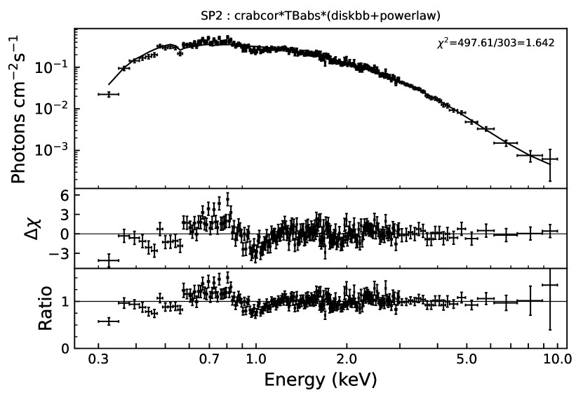
Figure 5: A spectral fit to representative dataset SP2, it demonstrates apparent emission and absorption features around 0.7 keV and 1.0 keV using model crabcor*TBabs*(diskbb+powerlaw). For visual clarity, data has been rebinned. Top: spectral data and model. Middle: standardized fit residuals. Bottom: data-to-model ratio.

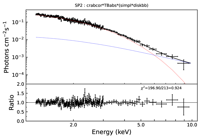
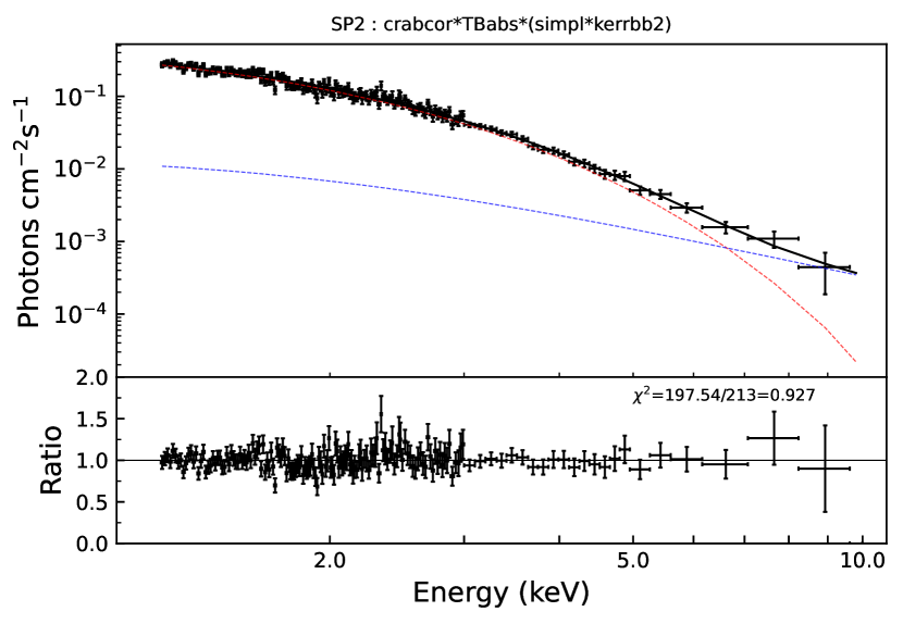
Figure 6: Spectral fits for SP2 in 1.2-10.0 keV with model crabcor*TBabs*(simpl*diskbb) and model crabcor*TBabs*(simpl*kerrbb2). The red dashed line represents the thermal component and the blue dashed line represents the Comptonization component. For visual clarity, data has been rebinned.

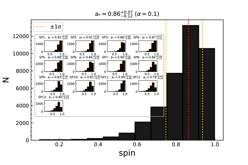
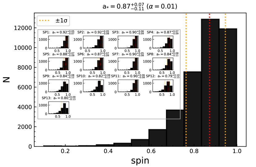
Figure 7: a) For $\alpha=0.1$, the total histogram of $a_{*}$ for SP1-SP13, with 39,000 data points. The red dotted lines indicate the center value of $a_{*}$, while the orange dotted lines show the $\pm 68.3\%$ ($\pm$ 1$\sigma$). The insert of Figure 7 is spin results adopting $\alpha=0.1$, from SP1 to SP13, showing the results of the respective MC analyses. b) Same as Figure 7, except for $\alpha=0.01$.

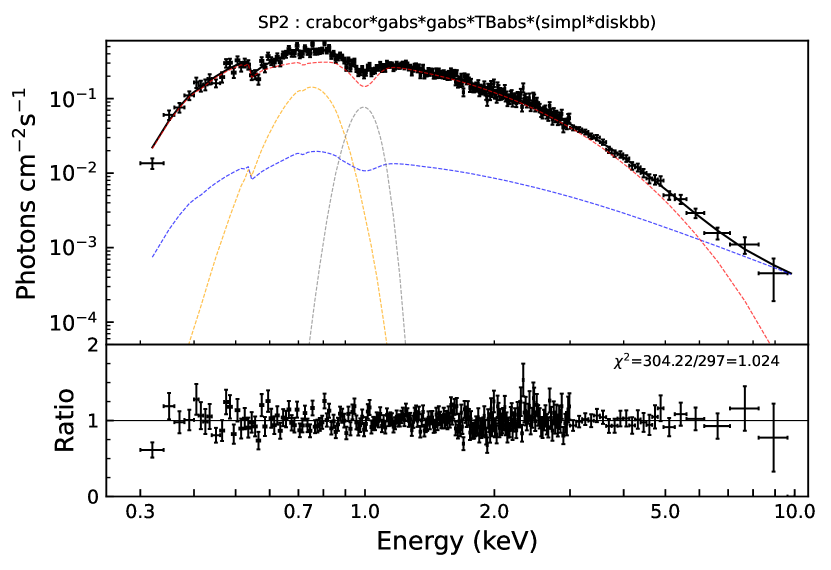
Figure 8: Spectral fits for SP2 in 0.3-10.0 keV with model crabcor*gabs*gabs*TBabs*(simpl*diskbb) and model crabcor*gabs*gabs*TBabs*(simpl*kerrbb2). The red dashed line represents the thermal component, the blue dashed line represents the Comptonization component, the yellow dotted line represents the emission line, and the gray dotted line represents the absorption line. For visual clarity, data has been rebinned.

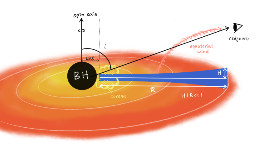
Figure 9: Equatorial wind illustration. Black represents the central black hole. Blue shows a schematic cross-section depicting the scale-height ratio H/R $\ll$ 1 for the geometrically-thin disk. Pink represents the equatorial wind. The central BH does likely illuminate the outer disk, and as a result, it may heat the outer disk, increasing the thermal pressure that forces away the wind that is flattened above the disk. Because of this, the wind is most readily detected for a high inclination case.

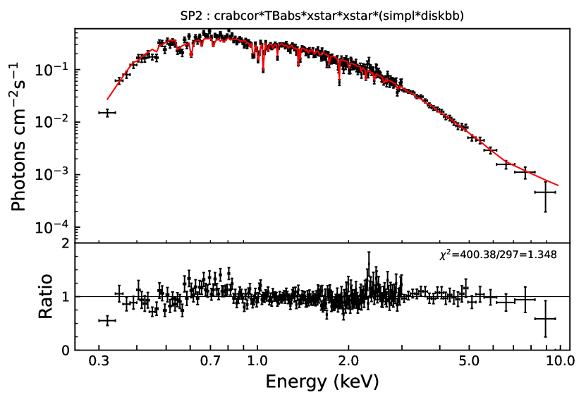
Figure 10: Spectral fits for SP2 from 0.3-10.0 keV with model crabcor*TBabs*xstar*(simpl*diskbb) and model crabcor*TBabs*xstar*xstar*(simpl*diskbb). For visual clarity, data has been rebinned.

3 SPECTRAL ANALYSIS AND RESULTS

Regardless of its selection or rejection by screening conditions, a preliminary and simplistic spectral model: crabcor*TBabs*(diskbb+powerlaw) is applied to all data to assess each spectrum in 0.3-10.0 keV, over which Swift/XRT is sensitive. To account for the considerable flux-normalization discrepancies amongst X-ray missions, we follow prior work (Steiner et al. 2010) and standardize the calibration using the Crab as a reference. According to https://www.swift.ac.uk/analysis/xrt/digest_cal.php#abs, we find the parameter values of Crab for Swift, and use $\Gamma=2.1$, $N=9.7\text{ photons }s^{-1}\text{keV}^{-1}$ (Toor & Seward 1974) as the standard values. Then we compute the normalization-correction coefficient $C_{\mathrm{TS}}$ is 0.948, and the slope difference $\Delta\Gamma_{\mathrm{TS}}$ is 0. The model crabcor is used to implement this standardization in XSPEC. We adopt Tbabs as the interstellar absorption model (for the interstellar medium, the photoionization cross-sections are based on Verner et al. 1996, and the abundances are based on Wilms et al. 2000). We fix the hydrogen column density ($N_{\mathrm{H}}$) to $1.8\times 10^{21}\mathrm{cm^{-2}}$, which is the average of preliminary fits using free $N_{\mathrm{H}}$ for all data with model crabcor*TBabs*(diskbb+powerlaw). It is also highly consistent with the total Galactic column density: https://heasarc.gsfc.nasa.gov/cgi-bin/Tools/w3nh/w3nh.pl. As seen in Figure 5, there are two confounding emission/absorption components around 0.7 and 1.0 keV, respectively. In Section 4.2 we examine potential wind models that explain these features and discuss their importance and impact on the spin. However, in our primary analysis, we here opt to omit this problematic energy range and perform our analysis over 1.2-10.0 keV.

In summary, we perform a fit using the model crabcor*TBabs*(simpl*diskbb) for all stable data sets > 200s and RMS < 0.075, we use the resultant $f_{\mathrm{sc}}$ values as our final screening condition in 1.2-10.0 keV (see Section 3.1 for details). We list $f_{\mathrm{sc}}$ only for a subset who meets the RMS <0.075 and the light-curve is stable in the last column of Table 1. We end up with a total of 13 “gold" spectra that meet all these conditions. In addition, we also show the results of the fit for “gold" spectra using the powerlaw model in Table 2.

Table 2: The best-fitting parameters with crabcor*TBabs*(diskbb+powerlaw)

Spec.	ObsID	Seg.	diskbb		powerlaw1	$\chi^{2}_{\nu}$	$\chi^{2}$(d.o.f.)	DF
			$T_{\rm in}$	$\rm norm$ $(\times 10^{2})$	$\rm norm$ $(\times 10^{-2})$
			($\rm keV$)		($\rm photons~{}\mathrm{keV^{-1}}\mathrm{cm^{-2}}\mathrm{s^{-1}}$ )			$(\%$)
SP1	00032339015	Seg2	0.862 $\pm$ 0.011	1.61 $\pm$ 0.07	13.31 $\pm$ 1.69	1.053	226.29/215	76.98
SP2	00032461008	Seg1	0.774 $\pm$ 0.011	2.14 $\pm$ 0.10	6.56 $\pm$ 1.27	0.921	196.24/213	84.43
SP3	00032461008	Seg2	0.755 $\pm$ 0.012	2.30 $\pm$ 0.13	9.20 $\pm$ 1.34	1.009	214.97/213	78.72
SP4	00032339028	Seg1	0.729 $\pm$ 0.008	2.63 $\pm$ 0.10	10.21 $\pm$ 0.92	1.054	226.56/215	76.32
SP5	00032461011	Seg2	0.722 $\pm$ 0.008	2.62 $\pm$ 0.11	7.92 $\pm$ 0.86	0.997	213.36/214	79.74
SP6	00032461012	Seg1	0.718 $\pm$ 0.009	2.86 $\pm$ 0.12	9.03 $\pm$ 0.97	1.083	231.80/214	78.64
SP7	00032339030	Seg1	0.709 $\pm$ 0.015	1.77 $\pm$ 0.14	11.65 $\pm$ 1.14	1.113	237.02/213	62.40
SP8	00032461013	Seg1	0.749 $\pm$ 0.010	1.88 $\pm$ 0.09	22.40 $\pm$ 1.07	1.010	219.10/217	54.38
SP9	00032461014	Seg1	0.727 $\pm$ 0.010	2.38 $\pm$ 0.11	17.49 $\pm$ 1.08	0.983	212.22/216	62.62
SP10	00032461014	Seg2	0.725 $\pm$ 0.009	2.50 $\pm$ 0.11	19.92 $\pm$ 1.03	1.044	226.60/217	60.35
SP11	00032461015	Seg1	0.705 $\pm$ 0.017	1.85 $\pm$ 0.16	11.14 $\pm$ 1.27	0.962	203.87/212	63.76
SP12	00032461015	Seg3	0.738 $\pm$ 0.014	2.46 $\pm$ 0.16	26.32 $\pm$ 1.83	1.052	226.20/215	55.37
SP13	00032461017	Seg1	0.701 $\pm$ 0.014	1.78 $\pm$ 0.12	25.29 $\pm$ 1.11	1.144	247.19/216	42.14

• 1 Gamma fixed at 2.2.

• Notes. In columns 4-9, we show the temperature of the inner disk radius ($T_{\rm in}$) in units of keV, the disk component’s amplitude (norm), the normalization of power-law at 1.0 keV, the reduced chi-square ($\chi^{2}_{\nu}$), the total chi-square ($\chi^{2}$) and the degrees of freedom (d.o.f.), disk fraction (DF) gives the proportion of unabsorbed flux in the thermal component over the energy range from 1.2 to 10.0 keV. The errors are calculated in 68.3% confidence intervals by XSPEC.

3.1 The non-relativistic spectral model

All “gold" spectra are fitted to a Comptonized multicolor disk blackbody (MCD) model with interstellar absorption. For the MCD, we use the diskbb model (Mitsuda et al. 1984; Makishima et al. 1986), and for Compton scattering, we use the simpl model (Steiner et al. 2009a; Steiner et al. 2009b). We are unable to robustly constrain the photon index $\Gamma$ of the simpl model due to inadequate statistics in the hard X-ray band for much of the data. As a result, we fix $\Gamma$ to 2.2, which is a typical value for BHXRBs in the soft state (e.g., Kolehmainen et al. 2011). For the model simpl, we use the energies command in XSPEC to expand the sampled energies to 0.1-100.0 keV (see the appendix of Steiner et al. 2009b). The non-relativistic composite model crabcor*TBabs*(simpl*diskbb) is used. The best-fitting findings for SP1-SP13 are shown in Table 3. These 13 spectra are well fitted, and the reduced chi-square $\chi^{2}_{\nu}$ of SP1-SP13 are concentrated around 1. Figure 6 depicts the fitting of SP2 as a representation. We can easily see that the model fits well with no significant residuals.

Table 3: The best-fitting parameters with crabcor*TBabs*(simpl*diskbb)

Spec.	ObsID	Seg.	simpl	diskbb		$\chi^{2}_{\nu}$	$\chi^{2}$(d.o.f.)
			$f_{\rm sc}$	$T_{\rm in}~{}(\rm keV)$	$\rm norm$ $(\times 10^{2})$
SP1	00032339015	Seg2	0.098 $\pm$ 0.012	0.804 $\pm$ 0.014	2.51 $\pm$ 0.17	0.983	211.31/215
SP2	00032461008	Seg1	0.051 $\pm$ 0.010	0.754 $\pm$ 0.013	2.62 $\pm$ 0.18	0.924	196.90/213
SP3	00032461008	Seg2	0.072 $\pm$ 0.011	0.727 $\pm$ 0.014	3.08 $\pm$ 0.23	0.998	212.51/213
SP4	00032339028	Seg1	0.076 $\pm$ 0.007	0.703 $\pm$ 0.009	3.57 $\pm$ 0.18	1.080	232.14/215
SP5	00032461011	Seg2	0.064 $\pm$ 0.007	0.700 $\pm$ 0.009	3.37 $\pm$ 0.18	1.002	214.53/214
SP6	00032461012	Seg1	0.067 $\pm$ 0.008	0.696 $\pm$ 0.010	3.72 $\pm$ 0.21	1.098	234.93/214
SP7	00032339030	Seg1	0.134 $\pm$ 0.014	0.660 $\pm$ 0.016	3.10 $\pm$ 0.30	1.105	235.38/213
SP8	00032461013	Seg1	0.181 $\pm$ 0.009	0.669 $\pm$ 0.010	4.28 $\pm$ 0.26	0.939	203.80/217
SP9	00032461014	Seg1	0.135 $\pm$ 0.009	0.675 $\pm$ 0.010	4.21 $\pm$ 0.25	0.962	207.76/216
SP10	00032461014	Seg2	0.147 $\pm$ 0.008	0.667 $\pm$ 0.009	4.70 $\pm$ 0.26	0.974	211.33/217
SP11	00032461015	Seg1	0.126 $\pm$ 0.015	0.660 $\pm$ 0.018	3.11 $\pm$ 0.34	0.955	202.46/212
SP12	00032461015	Seg3	0.171 $\pm$ 0.012	0.667 $\pm$ 0.014	5.29 $\pm$ 0.45	1.072	230.42/215
SP13	00032461017	Seg1	0.239 $\pm$ 0.011	0.604 $\pm$ 0.013	5.49 $\pm$ 0.45	1.157	250.00/216

• Notes. Columns 4-9 show the scattered fraction ($f_{\rm sc}$), the temperature of the inner disk radius ($T_{\rm in}$) in units of keV, the disk component’s amplitude (norm), the reduced chi-square ($\chi^{2}_{\nu}$), the total chi-square ($\chi^{2}$) and the degrees of freedom (d.o.f.). The errors are calculated in 68.3$\%$ confidence interval by XSPEC.

3.2 The relativistic spectral model

Having now explored the data using preliminary non-relativistic models, we turn to the relativistic accretion disk model kerrbb2 (McClintock et al. 2006). kerrbb2 is a combination of the disk models bhspec and kerrbb. bhspec is used to derive the spectral hardening factor $f\equiv T\mathrm{col/T\mathrm{eff}}$ (Davis et al. 2005), whilst kerrbb is used to model the disk using ray-tracing computations (Li et al. 2005). We begin by generating spectral-hardening look-up tables using bhspec with a default viscosity parameter value $\alpha=0.1$ as a conservative estimate. The $f$-table is read in and used to automatically set the value of $f$ during kerrbb2 as a function of $\dot{M}$ and $a_{*}$. The complete model can be expressed as crabcor*TBabs*(simpl*kerrbb2). For model kerrbb2, the self-irradiation of the disk (rflag=1) and the influence of limb-darkening (lflag=1) are taken into account. And we also set the torque at the inner boundary of the disk to zero (eta=0). Table 4 summarizes our results, which implies that a moderate spin is most plausible. We can also see from the findings of $L/L_{\mathrm{Edd}}$ in Table 4 that it is in accordance with our demands of the disk being geometrically thin by requiring that the dimensionless luminosity <  0.3 (McClintock et al. 2014).

Table 4: The best-fitting parameters with the relativistic model crabcor*TBabs*(simpl*kerrbb2)

viscosity	Spec.	ObsID	Seg.	simpl	kerrbb2		$\chi^{2}_{\nu}$	$\chi^{2}$(d.o.f.)	$L/L_{\mathrm{Edd}}$
$\alpha$				$f_{\rm sc}$	$a_{*}$	$\dot{M}~{}(\times 10^{18}\mathrm{~{}g}\mathrm{~{}s}^{-1})$
	SP1	00032339015	Seg2	0.079 $\pm$ 0.012	0.917 $\pm$ 0.009	0.138 $\pm$ 0.006	1.037	222.87/215	0.018
	SP2	00032461008	Seg1	0.037 $\pm$ 0.010	0.909 $\pm$ 0.009	0.117 $\pm$ 0.005	0.927	197.53/213	0.015
	SP3	00032461008	Seg2	0.059 $\pm$ 0.011	0.884 $\pm$ 0.011	0.131 $\pm$ 0.006	1.023	217.87/213	0.015
	SP4	00032339028	Seg1	0.063 $\pm$ 0.007	0.863 $\pm$ 0.010	0.143 $\pm$ 0.005	1.065	228.98/215	0.016
	SP5	00032461011	Seg2	0.052 $\pm$ 0.007	0.875 $\pm$ 0.008	0.128 $\pm$ 0.004	1.004	214.82/214	0.014
	SP6	00032461012	Seg1	0.054 $\pm$ 0.007	0.856 $\pm$ 0.010	0.147 $\pm$ 0.005	1.090	233.18/214	0.016
0.1	SP7	00032339030	Seg1	0.120 $\pm$ 0.013	0.899 $\pm$ 0.014	0.084 $\pm$ 0.005	1.109	236.18/213	0.010
	SP8	00032461013	Seg1	0.164 $\pm$ 0.010	0.839 $\pm$ 0.010	0.153 $\pm$ 0.005	0.964	209.08/217	0.016
	SP9	00032461014	Seg1	0.120 $\pm$ 0.009	0.836 $\pm$ 0.010	0.157 $\pm$ 0.005	0.979	211.41/216	0.016
	SP10	00032461014	Seg2	0.130 $\pm$ 0.007	0.817 $\pm$ 0.013	0.176 $\pm$ 0.006	1.013	219.91/217	0.017
	SP11	00032461015	Seg1	0.113 $\pm$ 0.014	0.896 $\pm$ 0.017	0.086 $\pm$ 0.006	0.960	203.56/212	0.010
	SP12	00032461015	Seg3	0.151 $\pm$ 0.013	0.787 $\pm$ 0.018	0.214 $\pm$ 0.010	1.057	227.25/215	0.020
	SP13	00032461017	Seg1	0.219 $\pm$ 0.011	0.797 $\pm$ 0.017	0.145 $\pm$ 0.007	1.139	246.12/216	0.014
	SP1	00032339015	Seg2	0.080 $\pm$ 0.012	0.924 $\pm$ 0.008	0.134 $\pm$ 0.006	1.035	222.47/215	0.018
	SP2	00032461008	Seg1	0.037 $\pm$ 0.010	0.917 $\pm$ 0.009	0.112 $\pm$ 0.005	0.927	197.50/213	0.014
	SP3	00032461008	Seg2	0.058 $\pm$ 0.010	0.896 $\pm$ 0.012	0.126 $\pm$ 0.006	1.022	217.68/213	0.015
	SP4	00032339028	Seg1	0.064 $\pm$ 0.007	0.873 $\pm$ 0.008	0.139 $\pm$ 0.004	1.064	228.75/215	0.016
	SP5	00032461011	Seg2	0.052 $\pm$ 0.007	0.882 $\pm$ 0.008	0.125 $\pm$ 0.004	1.004	214.86/214	0.014
	SP6	00032461012	Seg1	0.054 $\pm$ 0.007	0.863 $\pm$ 0.011	0.144 $\pm$ 0.006	1.089	233.09/214	0.016
0.01	SP7	00032339030	Seg1	0.120 $\pm$ 0.014	0.907 $\pm$ 0.014	0.082 $\pm$ 0.005	1.108	236.11/213	0.010
	SP8	00032461013	Seg1	0.163 $\pm$ 0.009	0.844 $\pm$ 0.010	0.150 $\pm$ 0.005	0.964	209.12/217	0.016
	SP9	00032461014	Seg1	0.120 $\pm$ 0.009	0.842 $\pm$ 0.010	0.154 $\pm$ 0.005	0.979	211.48/216	0.016
	SP10	00032461014	Seg2	0.130 $\pm$ 0.008	0.825 $\pm$ 0.013	0.172 $\pm$ 0.006	1.012	219.65/217	0.017
	SP11	00032461015	Seg1	0.114 $\pm$ 0.015	0.905 $\pm$ 0.016	0.083 $\pm$ 0.006	0.960	203.45/212	0.010
	SP12	00032461015	Seg3	0.151 $\pm$ 0.013	0.795 $\pm$ 0.018	0.210 $\pm$ 0.010	1.057	227.24/215	0.020
	SP13	00032461017	Seg1	0.220 $\pm$ 0.011	0.805 $\pm$ 0.018	0.142 $\pm$ 0.007	1.140	246.15/216	0.014

• Notes. Columns 5-10 show the scattered fraction ($f_{\rm sc}$), the dimensionless spin parameter ($a_{*}$), the mass accretion rate through the disk in units of 10¹⁸ g s ^-1 ($\dot{M}$), the reduced chi-square ($\chi_{\nu}^{2}$), the total chi-square ($\chi^{2}$) and the degrees of freedom (d.o.f.), the bolometric Eddington-scaled luminosity ($L/L_{\mathrm{Edd}}$, where $L_{\mathrm{Edd}}=1.3\times 10^{38}\left(M/M_{\odot}\right)$ erg $\mathrm{s}^{-1}$). The errors are calculated in 68.3$\%$ confidence interval by XSPEC. For these fits, the system parameters are $M_{\rm BH}=8.9_{-1.0}^{+1.6}M_{\odot}$, $D=7.5_{-1.4}^{+1.8}\mathrm{kpc}$, and $i={72_{-8}^{+5}}^{\circ}$ (uncertainties are 1 $\sigma$; Mata Sánchez et al. 2021).

3.3 Comprehensive spin error analysis

In this section, we consider various sources of observational error, both systematic and statistical (See Section 5 and Appendix A in Steiner et al. 2011; Section 5 in McClintock et al. 2014 for details), that have an impact on our final estimate of the spin. They are (1) the uncertainties from the analytic Novikov-Thorne model and the disk atmosphere model; For MAXI J1305-704, these model errors are especially small because of the low luminosity of the disk, and so we do not explore its effect in this paper. (2) the effect of the emission/absorption lines in low-energy bands (discussion see Section 4.1); (3) the effect of hydrogen column density $N_{\mathrm{H}}$ (discussion see Section 4.2); (4) the influence of the fixed photon index $\Gamma$ (discussion see Section 4.3); (5) the influence of viscosity parameter $\alpha$ (discussion see Section 4.4); (6) X-ray flux calibration uncertainties; In general, we need to include the uncertainty in the luminosity due to the $\sim$10% uncertainty in the flux of the Crab (Toor & Seward 1974). But for MAXI J1305-704, the effect of the uncertainty in the absolute flux calibration is much smaller in impact compared to the 24% uncertainty in $D$, which is equivalent to a 48% uncertainty in the measurement of flux. Therefore, absolute X-ray flux calibration uncertainties are of minor importance compared to the uncertainties in the input system parameters. and (7) the uncertainties in the input parameters $M$, $i$, and $D$. Specifically, as in earlier works (Liu et al. 2008; Gou et al. 2009), we employ Monte Carlo (MC) approach to assess the uncertainties in the CF method, from uncertainty in the dynamical inputs ($M$, $i$, $D$). Due to the measurement correlations between $M$ and $i$, the mass function $f(M)=M^{3}\sin^{3}i/\left(M_{\mathrm{opt}}+M\right)^{2}$ (where $M$ is the mass of the black hole, $M_{\mathrm{opt}}$ is the mass of the optical companion, and $i$ is the accretion disk inclination) is used to draw random parameters, as described in Gou et al. 2011. Specifically, we adopt $M_{\mathrm{opt}}=0.43\pm 0.16M_{\odot}$ (Mata Sánchez et al. 2021) to generate 3000 sets of ($M_{\mathrm{opt}}$, $f(M)$, $i$, $D$) for SP1-SP13, assuming each parameter is independent and has a Gaussian distribution. For each ($M_{\mathrm{opt}}$, $f(M)$, $i$), we determine $M$ via the mass function so that the parameters in these sets become ($M$, $i$, $D$). Then, for each set of parameters, we calculate $f$ via look-up tables with the viscosity parameter $\alpha$ fixed at 0.1 and 0.01 separately. Finally, we fit 3000 data sets to the composite model crabcor*TBabs*(simpl*kerrbb2) (see Section 3.2) to obtain the spin distribution and quantify the errors. The MC-determined error analysis of each spectrum is depicted in the inset of Figure 7 ($\alpha$=0.1) and 7 ($\alpha$=0.01). The histograms of $a_{*}$ for SP1-SP13 are depicted in Figure 7 ($\alpha$=0.1) and 7 ($\alpha$=0.01). Values and their 1 $\sigma$ equivalent uncertainties depict the mode and 68% confidence interval centered on the mode. [median is the value in the middle, and the mode is the high point of a Gaussian distribution.] Consequently, we perform a comprehensive analysis in which we find that the spin of MAXI J1305-704 has an acceptable range of 0.74-0.95 (1 sigma confidence interval). We find that the individual spectra exhibit surprising variance in their spin determination (compared to other sources); many are centered on moderate values whereas others seem to favor the maximum spin. Since the 13 spectra we selected are stable, such differences are not due to variability. Possible reasons are discussed in detail in Section 4.5.

4 DISCUSSIONS

4.1 The influence of the low energy band

4.1.1 Adding simplistic gaussian models: gabs

Here we examine the impact of the low-energy features on our fitting results by alternatively considering empirical and physical models for their origin. We begin using a simplistic Gaussian model (gabs) to capture the two low-energy features, and by allowing both positive and negative normalizations allow for features to be either emission or absorption. For 0.3-10.0 keV, the complete non-relativistic model is crabcor*gabs*gabs*TBabs*(simpl*diskbb), and the complete relativistic model is crabcor*gabs*gabs*TBabs*(simpl*kerrbb2). To facilitate comparison, we take SP2 as our touchstone example, which is representative of the full “gold" data sets. We can see from Figure 8 and 8 that the data fits are of similar quality and character using both non-relativistic and relativistic models. The best-fit results are listed in Table 5. From the fourth and fifth columns of Table 5 (Models A and B, respectively), we can see that when fitting to different energy bands, $f_{\rm sc}$ and $T_{\rm in}$ remain the same. Similarly, columns 6 and 7 show that with Models C and D, we can see that the spin changes by 3%. These results suggest that ignoring the lowest energies has a minor impact on the fit results, and is a reasonable simplification.

Table 5: The best-fitting parameters for SP2 in both energy bands

Component	Parameter	Description	A	B	C	D	E	F
			1.2-10.0 keV	0.3-10.0 keV	1.2-10.0 keV ($\alpha=0.1$)	0.3-10.0 keV ($\alpha=0.1$)	0.3-10.0 keV	0.3-10.0 keV
gabs1	$E_{\text{line }}(\mathrm{keV})$	line energy	…	0.74 $\pm$0.02	…	0.75$\pm$0.02	…	…
	$\sigma_{\text{line }}(\times 10^{-2}~{}\mathrm{keV})$	line width	…	9.7 $\pm$2.9	…	8.0 $\pm$2.8	…	…
	$\tau~{}(\times 10^{-2})$	line depth	…	-8.9 $\pm$2.1	…	-6.5 $\pm$1.6	…	…
gabs2	$E_{\text{line }}(\mathrm{keV})$	line energy	…	1.00 $\pm$0.03	…	1.00 $\pm$0.02	…	…
	$\sigma_{\text{line }}(\times 10^{-2}~{}\mathrm{keV})$	line width	…	6.4 $\pm$2.7	…	6.8 $\pm$2.4	…	…
	$\tau~{}(\times 10^{-2})$	line depth	…	4.5 $\pm$1.7	…	5.0 $\pm$1.4	…	…
xstar1	$N(\times 10^{22}\mathrm{~{}cm}^{-2})$	column density	…	…	…	…	6.0$\pm$2.9	4.1$\pm$0.9
	$\log\xi(\times\mathrm{erg}\mathrm{~{}cm}\mathrm{~{}s}^{-1}/s)$	ionization	…	…	…	…	2.61$\pm$0.20	2.49$\pm$0.11
	z $(\times 10^{-2})$	gravitational red-shift	…	…	…	…	6.9$\pm$0.8	7.8$\pm$1.2
xstar2	$N(\times 10^{22}\mathrm{~{}cm}^{-2})$	column density	…	…	…	…	…	$13.74~{}(*)$
	$\log\xi$$(\mathrm{~{}erg}\mathrm{~{}cm}\mathrm{~{}s}^{-1})$	ionization	…	…	…	…	…	3.68$\pm$1.51
	z	gravitational red-shift	…	…	…	…	…	0$\pm$0.03
simpl	$f_{\rm sc}$	the scattered fraction	0.051 $\pm$ 0.010	0.049$\pm$0.010	0.037 $\pm$ 0.010	0.034$\pm$ 0.010	0.062$\pm$0.009	0.067$\pm$0.011
diskbb	$T_{\rm in}~{}(\mathrm{keV})$	the temperature of the inner disk radius	0.754 $\pm$ 0.013	0.757$\pm$0.013	…	…	0.705$\pm$0.010	0.699$\pm$0.011
	$\rm norm$ $(\times 10^{2})$	normalization	2.62 $\pm$ 0.18	2.59 $\pm$ 0.17	…	…	4.06$\pm$0.22	4.42$\pm$0.87
kerrbb2	$a_{*}$	the dimensionless spin parameter	…	…	0.909 $\pm$ 0.009	0.936$\pm$0.007	…	…
	$\dot{M}~{}(\times 10^{18}\mathrm{~{}g}\mathrm{~{}s}^{-1})$	the effective mass accretion rate of the disk	…	…	0.117 $\pm$ 0.005	0.101$\pm$0.004	…	…
$L/L_{\mathrm{Edd}}$	…	the bolometric Eddington-scaled luminosities	…	…	0.015	0.014	…	…
$\chi_{v}^{2}$	…	…	0.924	1.024	0.927	1.037	1.357	1.348
$\chi^{2}~{}(\mathrm{d.o.f.})$	…	…	196.90/213	304.22/297	197.54/213	307.85/297	407.12/300	400.38/297

• Notes. Model A is crabcor*TBabs*(simpl*diskbb) in 1.2-10.0 keV, while Model B is crabcor*gabs*gabs*TBabs*(simpl*diskbb) in 0.3-10.0
  keV. Model C is crabcor*TBabs*(simpl*kerrbb2) in 1.2-10.0 keV, and Model D is crabcor*gabs*gabs*TBabs*(simpl*kerrbb2) in 0.3-10.0
  keV. Model E is crabcor*TBabs*xstar*(simpl*diskbb) in 0.3-10.0 keV, and Model F is crabcor*TBabs*xstar*xstar*(simpl*diskbb) in
  0.3-10.0 keV. (*) indicates that the parameter is unconstrained; the central value of the fit is provided for reference.
  The errors are calculated in 68.3$\%$ confidence interval by XSPEC.

4.1.2 Considering the influence of equatorial wind

We note that the broadened low-energy features can not be explained by the instrumental origins, so we now examine more physically-rigorous models for the low-energy features, especially consideration of a wind origin. Equatorial winds in BHXRBs are commonly indicated by the presence of highly-ionized absorption lines. As in the case of the broad emission/absorption can plausibly be interpreted as relativistic disk lines (0.7 keV and 1.0 keV lines may be relativistic O VIII and Fe L lines respectively) due to the equatorial wind, similar winds were launched previously like in H1743-322 (Miller et al. 2006) and GRS 1915+105 (Ueda et al. 2009). This phenomenon is often found in high-inclination (also called edge-on view, as shown in Figure 1 of Moriyama et al. 2017) systems in the soft state (for more detailed information, see Ponti et al. 2012). We show a cartoon of the wind on the equatorial plane (see Figure 9), which can help to illustrate this process.

We also note that for MAXI J1305-704, broad emission/absorption line features are also observed at the low energy end in the Chandra gratings data (Miller et al. 2014), Suzaku (Shidatsu et al. 2013) and Swift (different from the “gold" spectra used in our text) observations. Miller et al. 2014 suggested that these features could be attributed to a failed disk wind which was assessed using a large XSTAR grid. We follow Miller et al. 2014’s analysis and construct similar (though lower-resolution) XSTAR grids, using the same settings. Specifically, we assume a simple unabsorbed incident spectrum of kT = 1.0 keV with a luminosity of $L=1.0\times 10^{37}\operatorname{erg~{}s}^{-1}$ in the energy range of 1-1000 Ry (1 Ry=13.6 eV). We use XSTAR v2.58e (Kallman & Bautista 2001) and assume a covering factor of $\Omega/4\pi=0.5$, turbulent velocity of $v=700\mathrm{~{}km}/\mathrm{s}$, and all elements of solar abundances. Then we construct a grid of 150 models, spanning $2.0\leq\log\xi$ (ionization) $\leq 4.5$, $5\times 10^{21}\mathrm{~{}cm}^{-2}\leq N$ (column density) $\leq 5\times 10^{23}\mathrm{~{}cm}^{-2}$, and $10^{16}\mathrm{~{}cm}^{-3}\leq n$ (density) $\leq 10^{18}\mathrm{~{}cm}^{-3}$. The fit is much improved by using crabcor*TBabs*xstar*(simpl*diskbb) in 0.3-10.0 keV, when assuming $n=10^{17}\mathrm{~{}cm}^{-3}$ (Miller et al. 2014). However, it is still far from being formally accepted as a statistical fit. The results of the fit are listed in the eighth column of Table 5. From Figure 10, we can clearly see that the residuals around 0.7 keV are not eliminated. We explore this deficiency by allowing for an additional zone by adding an additional XSTAR model. The full model is crabcor*TBabs*xstar*xstar*(simpl*diskbb). And also assuming $n=10^{17}\mathrm{~{}cm}^{-3}$. The fitting results are presented in Table 5 and Figure 10. The use of two XSTAR models did not significantly improve the 0.7 keV residuals compared to the use of only one. We conclude that the residuals at 0.7 and 1.0 keV are not well-fitted concurrently for two winds with equal density. Addressing this deficiency may be possible by using two XSTAR models with a large difference in density. However, such a detailed analysis of these features is outside the scope of our work. We note that where the present XSTAR models do not perfectly fit the spectrum, we still consider the influence of the ionized absorber(s) on the spin. We find that, taking SP2 as a representative example, the spin increases by $\Delta a_{*}=0.024$ with model crabcor*TBabs*xstar*xstar*(simpl*kerrbb2) ($\chi_{v}^{2}$=439.59/297=1.480) in $\alpha=0.1$ case.

4.2 The influence of hydrogen column density $N_{\mathrm{H}}$

To check if the hydrogen column density has any influence on the spin results, we explore a generous range of putative values for $N_{\mathrm{H}}$, such as 0.10, 0.30, and 0.40 in units of $10^{22}\mathrm{cm}^{-2}$. Table 6 shows the detailed fitting results. When $N_{\mathrm{H}}$ is increased from $1\times 10^{21}\mathrm{~{}cm}^{-2}$ to $4\times 10^{21}\mathrm{~{}cm}^{-2}$, $a_{*}$ for SP2 varies from 0.931 to 0.834, with $\Delta a_{*}$ equaling 0.107. Because a higher value for $N_{\mathrm{H}}$ implies that the intrinsic disk emission must be larger, the luminosity increases while the disk temperature is much more weakly affected. Accordingly, the inferred spin decreases with larger $N_{\mathrm{H}}$. In general, changing the value of $N_{\mathrm{H}}$ has a relatively small influence on the final spin outcomes when compared to the dynamical sources of uncertainty.

Table 6: When changing $N_{\mathrm{H}}$ for SP2, the best-fitting results with crabcor*TBabs*(simpl*kerrbb2)  ($\alpha=0.1$)

TBabs	simpl	kerrbb2		$\chi^{2}_{\nu}$	$\chi^{2}$(d.o.f.)	$L/L_{\mathrm{Edd}}$
$N_{\mathrm{H}}$ ($\times 10^{22}\mathrm{cm}^{-2}$)	$f_{\rm sc}$	$a_{*}$	$\dot{M}~{}(\times 10^{18}\mathrm{~{}g}\mathrm{~{}s}^{-1})$
0.10	0.032 $\pm$ 0.010	0.931 $\pm$ 0.008	0.101 $\pm$ 0.005	0.942	200.550/213	0.014
0.18	0.037 $\pm$ 0.010	0.909 $\pm$ 0.009	0.117 $\pm$ 0.005	0.927	197.530/213	0.015
0.30	0.045 $\pm$ 0.010	0.872 $\pm$ 0.011	0.144 $\pm$ 0.006	0.936	199.320/213	0.016
0.40	0.050 $\pm$ 0.009	0.834 $\pm$ 0.013	0.172 $\pm$ 0.007	0.969	206.330/213	0.018

• Notes. We display the following data: the hydrogen column density in units of $10^{22}\mathrm{cm}^{-2}$ ($N_{\mathrm{H}}$), the scattered fraction ($f_{\rm sc}$), the dimensionless spin parameter ($a_{*}$), the mass accretion rate of the disk in units of 10¹⁸ g s ^-1 ($\dot{M}$), the reduced chi-square ($\chi_{\nu}^{2}$), the total chi-square ($\chi^{2}$) and the degrees of freedom (d.o.f.), the bolometric Eddington-scaled luminosity ($L/L_{\mathrm{Edd}}$). The errors are calculated in 68.3$\%$ confidence interval by XSPEC.

4.3 The influence of the photon index $\Gamma$

To investigate the influence of $\Gamma$ on the spin, we tested $\Gamma$ by changing its value from 2.2 to 1.6, 1.8, 2.0, 2.4, 2.6, and 2.8. This is presented in Table 7 for SP2 as representative of the “gold" set. $a_{*}$ varies from 0.912 to 0.906 when $\Gamma$ is raised from 1.6 to 2.8, $\Delta a_{*}$ equaling 0.007. Ultimately, we find that the value of $\Gamma$ has a negligible influence on the final spin.

4.4 The influence of viscosity parameter $\alpha$

Although we present results for $\alpha$= 0.1 as our default in this work, we also complete the same computations for $\alpha=0.01$. Table 4 presents both sets of results, and we see that $\alpha=0.01$ yields slightly larger values for the spin (for $\alpha=0.01$, the average spin is 0.868 $\pm$ 0.039; for $\alpha=0.1$, the average spin is 0.860 $\pm$ 0.039), as expected, consistent with findings in other systems, e.g., Cygnus X-1 (Gou et al. 2011; Zhao et al. 2021). We adopt an averaging over $\alpha=0.01$ and $\alpha=0.1$ for the final result.

4.5 Discussion of the large variance in CF results

In MAXI J1305-704, there is a very unusual phenomenon, that is, it has a high inner disk temperature ($\sim$0.9 keV) but a low Eddington fraction ($\sim$0.02 $L_{\mathrm{Edd}}$) (Shidatsu et al. 2013; Morihana et al. 2013 similarly point out this anomaly). And at a given, fixed $M$, $i$, and $D$, the CF spin results show a substantially larger variance (0.74-0.95), which is anomalous vs other BHXRBs where that dispersion is very small compared to the spread introduced by the errors in $M$, $i$, and $D$. The typical variance in value is $\sim 3\%$ in radius, equivalent to $\Delta a_{*}\approx 0.05$ at $a_{*}=0$ or $\Delta a_{*}\approx 0.01$ at $a_{*}=0.9$. We speculatively suggest that these phenomena are coupled. The inner disk temperature of the diskbb component (see Table 2) is much higher than what is typical of a faint soft state in most BHXRBs with a low accretion rate. One possible reason is that the relativistic Doppler effects significantly modify the disk spectra due to the high inclination angle ($i={72_{-8}^{+5}}^{\circ}$; see Muñoz-Darias et al. (2013) to learn more). Or the high black hole spin significantly modifies the disk spectra. Meanwhile, due to the strong degeneracy between luminosity and spin, the large variance in CF results (which is an order of magnitude larger than usual) is plausibly related to its associated luminosity coupling and may also introduce noise into the continuum results for this system. We speculate that the strong and variable wind is at least partially responsible for the spin variations. The impact of disk winds on faint soft states for other high-inclination systems may be useful to assess this question in follow-up studies.

The spin distribution of low-mass X-ray binaries (LMXBs) is relatively scattered, ranging from high spin to medium spin to low spin. The spin results of MAXI J1305-704 are in general agreement with the spin distribution observed in LMXBs (Reynolds 2021; Bambi et al. 2021). In addition, Steiner et al. (2012) reported a possible underlying link between black hole spin and mechanical jet power.

Table 7: When changing $\Gamma$ for SP2, the best-fitting results with crabcor*TBabs*(simpl*kerrbb2)  ($\alpha=0.1$)

simpl		kerrbb2		$\chi^{2}_{\nu}$	$\chi^{2}$(d.o.f.)	$L/L_{\mathrm{Edd}}$
$\Gamma$	$f_{\rm sc}$	$a_{*}$	$\dot{M}~{}(\times 10^{18}\mathrm{~{}g}\mathrm{~{}s}^{-1})$
1.6	0.024 $\pm$ 0.006	0.912 $\pm$ 0.008	0.116 $\pm$ 0.005	0.925	197.01/213	0.015
1.8	0.027 $\pm$ 0.007	0.911 $\pm$ 0.008	0.116 $\pm$ 0.005	0.926	197.17/213	0.015
2.0	0.032 $\pm$ 0.008	0.910 $\pm$ 0.009	0.116 $\pm$ 0.005	0.927	197.36/213	0.015
2.2	0.037 $\pm$ 0.010	0.909 $\pm$ 0.009	0.117 $\pm$ 0.005	0.927	197.53/213	0.015
2.4	0.045 $\pm$ 0.012	0.908 $\pm$ 0.009	0.117 $\pm$ 0.005	0.928	197.76/213	0.015
2.6	0.053 $\pm$ 0.015	0.907 $\pm$ 0.010	0.117 $\pm$ 0.005	0.930	197.99/213	0.015
2.8	0.063 $\pm$ 0.017	0.906 $\pm$ 0.010	0.118 $\pm$ 0.005	0.931	198.21/213	0.015

• Notes. Columns 4-9 show the dimensionless photon index ($\Gamma$), the scattered fraction ($f_{\rm sc}$), the dimensionless spin parameter ($a_{*}$), the mass accretion rate of the disk in units of 10¹⁸ g s ^-1 ($\dot{M}$), the reduced chi-square ($\chi^{2}_{\nu}$), the total chi-square ($\chi^{2}$) and the degrees of freedom (d.o.f.), the bolometric Eddington-scaled luminosity ($L/L_{\mathrm{Edd}}$). The errors are calculated in 68.3$\%$ confidence interval by XSPEC.

5 CONCLUSIONS

We perform a spectroscopic analysis for the black hole that resides in MAXI J1305-704, utilizing Swift/XRT data in energy bands of 1.2-10.0 keV. We find that MAXI J1305-704 contains a moderate spin black hole with $a_{*}=0.87_{-0.13}^{+0.07}$ (1$\sigma$, averaging over $\alpha=0.1$ and $\alpha=0.01$) based on the model kerrbb2 and the system parameters of Mata Sánchez et al. 2021. Compared with other systems, MAXI J1305-704 is a relatively anomalous source with a larger-than-typical variance in CF spins, which is perhaps closely related to its unusually high-temperature disk at low ($\sim$2% $L_{\mathrm{Edd}}$) luminosities. It should be noted that our spin constraint is limited by the precision of the dynamical measurements; more precise dynamical measurements would improve the CF spin constraint using these Swift/XRT data.

DATA AVAILABILITY

This paper makes use of Swift/XRT archival data which can be acquired from HEASARC:
https://heasarc.gsfc.nasa.gov/cgi-bin/W3Browse/w3browse.pl

References

- Arnaud (1996) Arnaud K. A., 1996, in Jacoby G. H., Barnes J., eds, Astronomical Society of the Pacific Conference Series Vol. 101, Astronomical Data Analysis Software and Systems V. p. 17
- Bachetti et al. (2020) Bachetti M., et al., 2020, Zenodo
- Bambi et al. (2021) Bambi C., et al., 2021, Space Sci. Rev., 217, 65
- Bardeen et al. (1972) Bardeen J. M., Press W. H., Teukolsky S. A., 1972, ApJ, 178, 347
- Burrows et al. (2005) Burrows D. N., et al., 2005, Space Sci. Rev., 120, 165
- Cash (1979) Cash W., 1979, ApJ, 228, 939
- Charles et al. (2012) Charles P., Cornelisse R., Foster D., Casares J., Kotze M., Zdziarski A., 2012, The Astronomer’s Telegram, 4105, 1
- Chen et al. (2016) Chen Z., Gou L., McClintock J. E., Steiner J. F., Wu J., Xu W., Orosz J. A., Xiang Y., 2016, ApJ, 825, 45
- Davis et al. (2005) Davis S. W., Blaes O. M., Hubeny I., Turner N. J., 2005, ApJ, 621, 372
- Dong et al. (2020) Dong Y., García J. A., Liu Z., Zhao X., Zheng X., Gou L., 2020, MNRAS, 493, 2178
- Draghis et al. (2020) Draghis P. A., Miller J. M., Cackett E. M., Kammoun E. S., Reynolds M. T., Tomsick J. A., Zoghbi A., 2020, ApJ, 900, 78
- El-Batal et al. (2016) El-Batal A. M., et al., 2016, ApJ, 826, L12
- Fabian et al. (1989) Fabian A. C., Rees M. J., Stella L., White N. E., 1989, MNRAS, 238, 729
- García et al. (2018) García J. A., et al., 2018, ApJ, 864, 25
- Gou et al. (2009) Gou L. J., et al., 2009, ApJ, 701, 1076
- Gou et al. (2010) Gou L., McClintock J. E., Steiner J. F., Narayan R., Cantrell A. G., Bailyn C. D., Orosz J. A., 2010, The Astrophysical Journal, 718, L122
- Gou et al. (2011) Gou L., et al., 2011, ApJ, 742, 85
- Gou et al. (2014) Gou L. J., et al., 2014, ApJ, 790, 29
- Greiner et al. (2012) Greiner J., Rau A., Schady P., 2012, The Astronomer’s Telegram, 4030, 1
- Humphrey et al. (2009) Humphrey P. J., Liu W., Buote D. A., 2009, ApJ, 693, 822
- Kaastra & Bleeker (2016) Kaastra J. S., Bleeker J. A. M., 2016, A&A, 587, A151
- Kallman & Bautista (2001) Kallman T., Bautista M., 2001, ApJS, 133, 221
- Kennea et al. (2012a) Kennea J. A., et al., 2012a, The Astronomer’s Telegram, 4034, 1
- Kennea et al. (2012b) Kennea J. A., et al., 2012b, The Astronomer’s Telegram, 4044, 1
- Kennea et al. (2012c) Kennea J., Miller J. M., Beardmore A., Degenaar N., Reynolds M. T., 2012c, The Astronomer’s Telegram, 4071, 1
- Kolehmainen et al. (2011) Kolehmainen M., Done C., Díaz Trigo M., 2011, MNRAS, 416, 311
- Kubota & Done (2003) Kubota A., Done C., 2003, arXiv e-prints, pp astro–ph/0312493
- Leahy et al. (1983) Leahy D. A., Darbro W., Elsner R. F., Weisskopf M. C., Sutherland P. G., Kahn S., Grindlay J. E., 1983, ApJ, 266, 160
- Li et al. (2005) Li L.-X., Zimmerman E. R., Narayan R., McClintock J. E., 2005, ApJS, 157, 335
- Liu et al. (2008) Liu J. F., McClintock J. E., Narayan R., Davis S. W., Orosz J. A., 2008, ApJ, 679, L37
- Makishima et al. (1986) Makishima K., Maejima Y., Mitsuda K., Bradt H. V., Remillard R. A., Tuohy I. R., Hoshi R., Nakagawa M., 1986, ApJ, 308, 635
- Mata Sánchez et al. (2021) Mata Sánchez D., Rau A., Álvarez Hernández A., van Grunsven T. F. J., Torres M. A. P., Jonker P. G., 2021, MNRAS, 506, 581
- McClintock et al. (2006) McClintock J. E., Shafee R., Narayan R., Remillard R. A., Davis S. W., Li L.-X., 2006, ApJ, 652, 518
- McClintock et al. (2014) McClintock J. E., Narayan R., Steiner J. F., 2014, Space Sci. Rev., 183, 295
- Middleton et al. (2006) Middleton M., Done C., Gierliński M., Davis S. W., 2006, MNRAS, 373, 1004
- Miller et al. (2006) Miller J., et al., 2006, The Astrophysical Journal, 646, 394
- Miller et al. (2013) Miller J. M., et al., 2013, ApJ, 775, L45
- Miller et al. (2014) Miller J. M., et al., 2014, ApJ, 788, 53
- Mitsuda et al. (1984) Mitsuda K., et al., 1984, PASJ, 36, 741
- Miyamoto et al. (1991) Miyamoto S., Kimura K., Kitamoto S., Dotani T., Ebisawa K., 1991, ApJ, 383, 784
- Morihana et al. (2013) Morihana K., et al., 2013, PASJ, 65, L10
- Moriyama et al. (2017) Moriyama K., Mineshige S., Takahashi H. R., 2017, ApJ, 850, 56
- Morningstar & Miller (2014) Morningstar W. R., Miller J. M., 2014, ApJ, 793, L33
- Morningstar et al. (2014) Morningstar W. R., Miller J. M., Reis R. C., Ebisawa K., 2014, ApJ, 784, L18
- Muñoz-Darias et al. (2013) Muñoz-Darias T., Coriat M., Plant D. S., Ponti G., Fender R. P., Dunn R. J. H., 2013, MNRAS, 432, 1330
- Novikov & Thorne (1973) Novikov I. D., Thorne K. S., 1973, in Black Holes (Les Astres Occlus). pp 343–450
- Ponti et al. (2012) Ponti G., Fender R. P., Begelman M. C., Dunn R. J. H., Neilsen J., Coriat M., 2012, MNRAS, 422, L11
- Remillard & McClintock (2006) Remillard R. A., McClintock J. E., 2006, ARA&A, 44, 49
- Reynolds (2021) Reynolds C. S., 2021, ARA&A, 59, 117
- Sato et al. (2012) Sato R., et al., 2012, The Astronomer’s Telegram, 4024, 1
- Shidatsu et al. (2013) Shidatsu M., et al., 2013, ApJ, 779, 26
- Steiner et al. (2009a) Steiner J. F., McClintock J. E., Remillard R. A., Narayan R., Gou L., 2009a, ApJ, 701, L83
- Steiner et al. (2009b) Steiner J. F., McClintock J. E., Remillard R. A., Narayan R., Gou L., 2009b, ApJ, 701, L83
- Steiner et al. (2010) Steiner J. F., McClintock J. E., Remillard R. A., Gou L., Yamada S., Narayan R., 2010, ApJ, 718, L117
- Steiner et al. (2011) Steiner J. F., et al., 2011, MNRAS, 416, 941
- Steiner et al. (2012) Steiner J. F., McClintock J. E., Narayan R., 2012, The Astrophysical Journal, 762, 104
- Suwa et al. (2012) Suwa F., et al., 2012, The Astronomer’s Telegram, 4035, 1
- Tanaka & Lewin (1995) Tanaka Y., Lewin W. H. G., 1995, in X-ray Binaries. pp 126–174
- Toor & Seward (1974) Toor A., Seward F. D., 1974, AJ, 79, 995
- Ueda et al. (2009) Ueda Y., Yamaoka K., Remillard R., 2009, The Astrophysical Journal, 695, 888
- Verner et al. (1996) Verner D. A., Ferland G. J., Korista K. T., Yakovlev D. G., 1996, ApJ, 465, 487
- Wilms et al. (2000) Wilms J., Allen A., McCray R., 2000, ApJ, 542, 914
- Xu et al. (2018) Xu Y., et al., 2018, ApJ, 852, L34
- Zhang et al. (1995) Zhang W., Jahoda K., Swank J. H., Morgan E. H., Giles A. B., 1995, ApJ, 449, 930
- Zhang et al. (1997) Zhang S. N., Cui W., Chen W., 1997, ApJ, 482, L155
- Zhao et al. (2021) Zhao X., et al., 2021, ApJ, 908, 117