Metallicity-PAH Relation of MIR-selected Star-forming Galaxies in AKARI North Ecliptic Pole-wide Survey

Abstract

We investigate the variation in the mid-infrared spectral energy distributions of 373 low-redshift ($z<0.4$) star-forming galaxies, which reflects a variety of polycyclic aromatic hydrocarbon (PAH) emission features. The relative strength of PAH emission is parameterized as $q_{\mathrm{PAH}}$, which is defined as the mass fraction of PAH particles in the total dust mass. With the aid of continuous mid-infrared photometric data points covering 7-24 $\mu$m and far-infrared flux densities, $q_{\mathrm{PAH}}$ values are derived through spectral energy distribution fitting. The correlation between $q_{\mathrm{PAH}}$ and other physical properties of galaxies, i.e., gas-phase metallicity ($12+\mathrm{log(O/H)}$), stellar mass, and specific star-formation rate (sSFR) are explored. As in previous studies, $q_{\mathrm{PAH}}$ values of galaxies with high metallicity are found to be higher than those with low metallicity. The strength of PAH emission is also positively correlated with the stellar mass and negatively correlated with the sSFR. The correlation between $q_{\mathrm{PAH}}$ and each parameter still exists even after the other two parameters are fixed. In addition to the PAH strength, the application of metallicity-dependent gas-to-dust mass ratio appears to work well to estimate gas mass that matches the observed relationship between molecular gas and physical parameters. The result obtained will be used to calibrate the observed PAH luminosity-total infrared luminosity relation, based on the variation of MIR-FIR SED, which is used in the estimation of hidden star formation.

1 Introduction

Mid-infrared spectra of star-forming galaxies are frequently dominated by strong emission features at 3.3, 6.2, 7.7, 8.6, 11.3, and 12.7 $\mu$m from polycyclic aromatic hydrocarbon (PAH) molecules. PAHs contain more than tens to thousands carbon atoms as well as peripheral hydrogen atoms that produce emission through bending and stretching (see Tielens, 2008, for a review), and are considered to be an important component of the interstellar dust population. Since dust plays a significant role in the star-formation process by enhancing the formation of molecular hydrogen and being an efficient coolant of interstellar medium (ISM), PAHs are closely related to the star-formation activity. PAH emission features are observed in a broad range of astrophysical scales, including Galactic and extragalactic star-forming regions (e.g., Maragkoudakis et al., 2018; Knight et al., 2022), therefore the possibility of using PAH luminosity as star-formation rate (SFR) indicator has been intensively explored (e.g., Peeters et al., 2004; Calzetti et al., 2007; Lee et al., 2012; Shipley et al., 2016; Xie & Ho, 2019; Lai et al., 2020). The ubiquitous existence of PAH emission features in high-redshift (up to $z\sim 2$) galaxies (e.g., Elbaz et al., 2005; Lutz et al., 2005; Yan et al., 2005; Li, 2020) demonstrates potential for rest-frame MIR photometric or spectroscopic observations, such as probing the cosmic star-formation history in early universe (Lagache et al., 2004; Goto et al., 2010) and investigating the contribution of star formation in active galactic nuclei (AGN) host systems (Alonso-Herrero et al., 2020).

In order to establish the PAH-SFR correlation, the variation in PAH emissions in different ISM environments needs to be understood beforehand. One of the most well-studied factors relevant to the PAH variation is metallicity. It has been reported that PAH emission features are less prominent in low-metallicity environments (e.g., Engelbracht et al., 2005; Madden et al., 2006; Wu et al., 2006; Galliano et al., 2008). The emission features show negative correlation with the hardness of the radiation field (i.e., [Ne iii]/[Ne ii] ratios). In some cases, MIR spectra of ultraluminous infrared galaxies lack PAH emission features (Desai et al., 2006), indicating that these systems are dominated by AGN or are in a vigorous merging process (Yamada et al., 2013; Murata et al., 2017). It is suggested that PAH destruction may be more effective in low metallicity systems than in high metallicity systems, due to a hard radiation field and inefficient gas cooling. Another possibility is a low production of PAHs in low metallicity systems with low carbon abundance (Dwek, 2005), which is related to the evolution of carbon-rich TP-AGB stars (Galliano et al., 2008). The trend of PAH strength being dependent on the metallicity is also observed in galaxies at $z\sim 2$ (Shivaei et al., 2017), affecting a scaling relation between MIR and total IR luminosity that is frequently employed to estimate an attenuation-free SFR density based on the flux density measured using a single MIR photometric band.

Observations of local galaxies that are clearly detected in the MIR and FIR bands are used as the basis for building a dust emission model at MIR-FIR wavelengths. Based on the Spitzer and submillimeter observations of the SIRTF Nearby Galaxies Survey (SINGS; Kennicutt et al., 2003), Draine et al. (2007) have suggested that the dust-to-gas ratio in star-forming galaxies is dependent on the metallicity, and the PAH strength correlates with the metallicity as well. To parameterize the relative strength of PAH emission with respect to the total IR luminosity, Draine & Li (2007) dust emission model have defined the PAH index $q_{\mathrm{PAH}}$, i.e., fraction of dust mass locked within PAH molecules (with less than $10^{3}$ C atoms). In case of SINGS galaxies, the median $q_{\mathrm{PAH}}$ value of low-metallicity galaxies ($12+\mathrm{log(O/H)}<8.1$) is 1.0 %, while the value for high-metallicity galaxies ($12+\mathrm{log(O/H)}\geq 8.1$) is 3.55 %. The parameter $q_{\mathrm{PAH}}$ has also been applied to investigate MIR-FIR spectral energy distribution (SED) of Herschel Reference Survey galaxies (Ciesla et al., 2014). By presenting a positive correlation between $q_{\mathrm{PAH}}$ and oxygen abundance in a range of $8.2<12+\mathrm{log(O/H)}<8.5$, Ciesla et al. (2014) have suggested that $q_{\mathrm{PAH}}$ factor may provide metallicity constraint to galaxies ranging one-third solar metallicity to solar metallicity.

The aforementioned works are based on the studies of local ($<30$ Mpc) galaxies with a limited number of MIR photometry points. However, since the PAH spectrum is affected by several factors such as particle size and charge distribution (Smith et al., 2007; Maragkoudakis et al., 2020), flux densities in multiple MIR bands are required to better constrain the PAH luminosity and to identify PAH-luminous galaxies (e.g., Takagi et al., 2010). For example, in estimating $q_{\mathrm{PAH}}$ using SED fitting (Kovács et al., 2019), it is indicated that the addition of the 11, 15, and 18 $\mu$m bands of the AKARI/IRC is more advantageous than the use of single 22 or 24 $\mu$m band. Unfortunately, the majority of the galaxies described in Kovács et al. (2019) lack spectroscopic redshifts, and the use of photometric redshifts in SED fitting increases uncertainties in the derived physical parameters. MIR multiband survey data, complemented with optical spectroscopic observations and ancillary multiwavelength data especially equipped with FIR coverage, would allow us to probe the PAH strength variation of MIR-selected galaxies in terms of galaxy physical properties such as metallicity, SFR, and stellar mass.

In this paper, we present an analysis on the correlation between PAH abundance and gas-phase metallicity (i.e., oxygen abundance) of MIR-selected galaxies at $z<0.4$, using the continuous MIR photometry at 7-24 $\mu$m in addition to the FIR photometry at $\geq 250$ $\mu$m. Section 2 describes the characteristics of data we use and sample selection criteria. How metallicity and PAH mass fraction, as well as other physical properties of galaxies are measured is described in Sections 3 and 4, respectively. The results on the correlation between PAH and other factors are discussed in Section 5. Our work is summarized in Section 6. Throughout the paper, we use Planck 2018 cosmological parameters for a flat $\Lambda$CDM model (Planck Collaboration et al., 2020, $\Omega_{\rm m,0}=0.315$, $H_{0}=67.4\,$km s^-1 Mpc^-1).

2 Data and Sample

2.1 NEP-wide Multiwavelength Survey

The $\sim 5.4$ deg² region around the North Ecliptic Pole (NEP) has been observed by the infrared space telescope AKARI (Murakami et al., 2007), using nine near- to mid-IR filters of the Infrared Camera (IRC; N2, N3, N4, S7, S9W, S11, L15, L18W, L24) providing continuous wavelength coverage between 2 and 24 $\mu$m (NEP-wide survey; Kim et al., 2012). Numbers in the filter names represent the central wavelengths of the filters, while the “W” indicates wider filter width. The AKARI MIR bands provide information at wavelengths covering strong PAH emission lines (7.7, 8.6, 11.3 and 12.7 $\mu$m), making them good tools to estimate the PAH luminosity. Kim et al. (2012) and Kim et al. (2021) have provided catalogs of the sources detected in the AKARI/IRC. The numbers of the detected sources are different for different detection bands, e.g., $\sim 100,000$ in the NIR band (N3), $\sim 18,000$ in the S9W band and $\sim 4000$ in the L24 band. After excluding suspicious false detections that are related to cosmic-ray hits and data reduction artifacts, Kim et al. (2021) have finalized the NEP-wide catalog with 130,150 infrared sources that have detection in at least one of the AKARI/IRC nine bands. The $5\sigma$ flux limits in N2, N3, N4, S7, S9W, S11, L15, L18W, and L24 are 15.4, 13.3, 13.6, 58.6, 67.3, 93.8, 133.1, 120.2, and 274.4 $\mu$Jy, respectively.

Multiwavelength ancillary data sets are available in this region (see Kim et al. 2021 for a summary; Hwang et al., 2007; Jeon et al., 2014; Pearson et al., 2017; Nayyeri et al., 2018; Huang et al., 2020; Shim et al., 2020; Oi et al., 2021). The available dedicated multiwavelength observations and the legacy survey observations (using GALEX and WISE; Bianchi et al., 2017; Cutri et al., 2012) from ultraviolet to FIR wavelengths allow the exploration of the physical properties of MIR-selected galaxies, including redshift, SFR, stellar mass, and total IR luminosity. For example, Kim et al. (2021) have presented that 111,535 out of 130,150 AKARI sources have counterparts in the deep optical images obtained by Subaru/HSC (Oi et al., 2021). Among them, 19,674 sources are flagged to be associated with bad pixels, saturated pixels, and edges of the masked regions, which results the number of reliable AKARI sources with optical identification to be 91,861. Photometric redshifts of these 91,861 sources have been estimated by Ho et al. (2021) based on the template fitting using optical-NIR photometry. Target selection for optical spectroscopic observations in the following Section 2.2 utilizes the AKARI source catalog matched with optical source catalog.

Figure 1: (a) Comparison between the parent AKARI MIR-selected sources (dots) and sources with optical spectroscopic observations (crosses). Histograms on the top and the right show the number fractions of the sources with optical spectra among the entire MIR-selected sources, i.e., the completeness of the spectroscopic observations, for different magnitude bins. Optical spectra are available for more than 50% of the MIR-selected sources with $f_{\mathrm{S9W}}>0.4$ mJy (corresponds to $f_{\mathrm{S11}}>0.6$ mJy and/or $f_{\mathrm{L15}}>0.9$ mJy). (b) Redshift distributions of (i) AKARI MIR galaxies with optical identification (photometric redshifts from Ho et al., 2021), (ii) AKARI galaxies with $r$-band magnitude cut ($r<21.5$), (iii) MIR-selected sources targeted for optical spectroscopic observations using MMT/Hectospec and WIYN/Hydra, and (iv) $z_{\mathrm{spec}}<0.4$ sources studied in this work. All histograms are normalized to have equal areas. (c) Star-formation rate vs. stellar mass from SED fitting for AKARI galaxies with $z_{\mathrm{phot}}<0.4$ (dots), spectroscopic sample of galaxies with $z_{\mathrm{spec}}<0.4$ (open circles), and subsample of spectroscopic sample that also satisfy MIR and FIR detection criteria (crosses; see Section 2.4 for sample selection in this work). Overplotted solid lines represent star-forming main sequences at $z\sim 0$ and $z\sim 0.4$ (Speagle et al., 2014) with $\pm 0.2$ dex scatter as shaded regions. Short vertical and horizontal bars with different colors indicate median values of $\mathrm{log}\,M_{\mathrm{star}}$ and $\mathrm{log}\,\mathrm{SFR}$ for different samples, respectively.

2.2 Optical Spectroscopic Observations

Optical spectra of MIR-selected galaxies over the NEP-wide survey area have been obtained using the MMT/Hectospec and WIYN/Hydra multi-fiber spectrographs between 2008 and 2021, through the spectroscopic follow-up campaign of MIR sources. The earlier data using MMT/Hectospec and WIYN/Hydra (observed by 2008) have been published by Shim et al. (2013), where the targets are selected in 11 $\mu$m and 15 $\mu$m band (more than $10\sigma$ detection in both bands). Later in 2020 and 2021, spectroscopic observations of 9 $\mu$m-selected sources (with S9W magnitude brighter than 19.5 mag) have been carried out using MMT/Hectospec with the aim of increasing the number of MIR-selected sources with spectroscopic redshifts, which is essential for understanding the dependence of MIR-based star-formation activity as a function of galaxy environment (Hwang, H. S. et al. 2022, in preparation). The configurations for MMT/Hectospec observations in 2008 and 2021 are identical, i.e., using 270 lines mm^-1 grating to cover 3700-8500 Å  at a spectral resolution of $6\,$Å  with dispersion of 1.2 Å pixel^-1. The spectral resolution and dispersion of WIYN/Hydra spectra are similar to that of MMT/Hectospec. However, the quality of the WIYN/Hydra spectra in the wavelengths blueward of 4500 Å  is poor due to the low instrumental response.

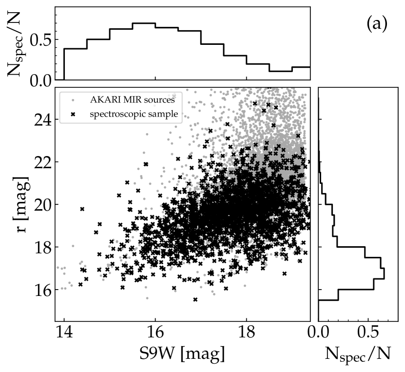
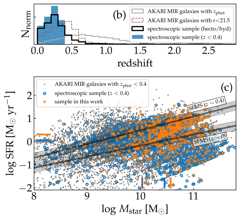
Figure 1a shows magnitude distribution of the parent AKARI MIR sources (91,861 sources from Kim et al. 2021) and the targets for optical spectroscopy in the $r$ vs. S9W plane. The approximate magnitude limit in optical ($r$-band) wavelength is $r=21.5$ mag, although some sources fainter than the $r$-band magnitude limit had a chance to occupy the spectroscopic fibers. The number fraction of the sources that have been selected for spectroscopic follow-up decreases as the $r$-band magnitude increases. At magnitudes of $\mathrm{S9W}<17.4$ (i.e., $f_{\mathrm{S9W}}>0.4$ mJy), about 50% of the AKARI sources are followed up for optical spectroscopic observations. In S11 and L15 bands, the flux limits where the 50% spectroscopic completeness is reached are $f_{\mathrm{S11}}>0.6$ mJy and $f_{\mathrm{L15}}>0.9$ mJy, respectively. The redshift distributions of the parent photometric sample and the spectroscopic sample are compared in Figure 1b. The parent sample plotted here represent 67,616 objects of which photometric redshifts are calculated and are classified as galaxies with better fits to galaxy template than stellar template (Ho et al., 2021). For the entire MIR sources, the median value of the redshift distribution is $\langle z_{\mathrm{phot}}\rangle=0.82$. If the $r$-band magnitude cut is applied, the value decreases with the decrease of the magnitude limit: $\langle z_{\mathrm{phot}}\rangle=0.38$, 0.27, and 0.18 for $r<21.5$, 20.5, and 19.5 mag. Considering that the spectroscopic sample completeness depends on the $r$-band magnitude, it is reasonable that the median redshift of the spectroscopic sample is lower than that of the photometric sample, i.e., $\langle z_{\mathrm{spec}}\rangle=0.22$.

The two representative physical properties, SFR and stellar mass, of the photometric and spectroscopic sample (both limited to redshift $z<0.4$) are illustrated in Figure 1c. Most sources are located on the previously known sequence of star-forming galaxies (e.g., Speagle et al., 2014) at $0<z<0.4$. The median values of $\mathrm{log}\,M_{\mathrm{star}}$ and $\mathrm{log}\,\mathrm{SFR}$ for different samples show that spectroscopic sample is composed of massive galaxies, as the sample consists of $r$-band bright sources. The median stellar mass of the $z<0.4$ photometric sample galaxies is $\langle\mathrm{log}\,M_{\mathrm{star}}[\mathrm{M}_{\odot}]\rangle=10$ while that of the spectroscopic sample galaxies is $\langle\mathrm{log}\,M_{\mathrm{star}}[\mathrm{M}_{\odot}]\rangle=10.4$. By applying Kolmogorov-Smirnov test, the stellar masses of the two samples are statistically different with a $p$-value less than 0.05. In case of the SFR, little difference is found for photometric and spectroscopic sample with the median values of $\langle\mathrm{log}\,\mathrm{SFR}[\mathrm{M}_{\odot}\,\mathrm{yr}^{-1}]\rangle=0.02$ and 0.04, respectively.

2.3 Emission Line Flux Measurement

Figure 2: (a) BPT diagram (Baldwin et al., 1981) for MIR-selected sources. Objects with sufficient MIR and FIR photometric data points (at least four in MIR wavelengths and one in FIR wavelengths) are marked as coral squares. Typical values of errors in $x$- and $y$-axes are plotted as an error bar at the bottom right. Overplotted are criteria to separate AGN and star-forming galaxies (Kewley et al. 2001 and Kauffmann et al. 2003 for solid and dashed lines, respectively). (b) MIR color-color diagram for AGN selection using WISE 3-bands (3.4, 4.6, and 12 $\mu$m) photometry. Dots are WISE-detected sources with spectroscopic redshifts of $z<0.4$. Objects that are classified by the BPT diagram as star-forming (H ii), composite, and AGN subgroups are plotted using different symbols. Typical error bar in both axes is shown in the right. Solid and dashed lines represent AGN selection criteria suggested by Mateos et al. (2012) and Jarrett et al. (2011), respectively, based on the assumption that AGN contribution is described by a power-law-shaped hot dust emission at 3-12 $\mu$m.

The extracted 1D spectra are flux-calibrated using the spectra of spectrophotometric standard stars that are simultaneously observed by filling the fibers in each observation configuration. Once the spectra are flux-calibrated and dereddened for Galactic extinction, spectroscopic redshifts are measured through template fitting. For line flux measurement, each spectrum is first visually inspected to check whether the spectroscopic redshift estimation is reasonable enough, then deredshifted into the rest frame using the spectroscopic redshift. Fluxes are measured for strong emission lines ([O ii], [O iii]$\lambda\lambda$4959, 5007, H$\alpha$, H$\beta$, [N ii]$\lambda\lambda$6548, 6584), applying a Gaussian profile fitting to the continuum-subtracted spectrum with the mpfit package based on the Levenberg-Marquardt method (Markwardt, 2009). The local continuum around each emission line is determined by the linear fit, except for the hydrogen lines where the stellar absorption is taken into account as a Gaussian with a broad FWHM and negative amplitude. For details of the redshift estimation and line flux measurement, please see Shim et al. (2013).

2.4 Sample Selection

The numbers of MIR-selected sources targeted for optical spectroscopic observations are 1155 (1796, including targets selected based on other selection criteria; Shim et al., 2013) and 1505, in observations that are obtained by 2008 and during the years 2020-2021, respectively. Since our motivation is to compare the gas-phase metallicity (measured in optical spectra) and the relative PAH strength to total dust luminosity (estimated from the MIR-FIR SED), we apply the following criteria for sample selection: (1) the object is detected in at least one of the Herschel/SPIRE bands (i.e., 250, 350, and 500 $\mu$m) with the flux density larger than the 10 mJy, (2) the object has at least four MIR photometric points at wavelengths between 7 and 24 $\mu$m, and (3) emission lines of H$\alpha$ and [N ii]$\lambda$6584 are clearly detected (i.e., S/N$\geq 3$) in the spectrum of the object.

The existence of flux density at wavelengths longer than the rest frame $100\,\mu$m is essential to constrain the total IR luminosity, since those wavelengths sample beyond the peak of the cold dust emission inside a galaxy. We measure flux densities in Herschel/SPIRE 250, 350, and 500 $\mu$m mosaic maps provided by the Herschel Extragalactic Legacy Project (Shirley et al., 2021) using the deblender tool xid+ (Hurley et al., 2017) with the optical source coordinates as priors. The use of a de-blender tool at a source position allows measurement of fluxes of sources that are not detectable by a blind source detection over several times the rms level. Nevertheless, in principle it is unreliable to probe below the confusion limit of the Herschel/SPIRE (Nguyen et al., 2010). Therefore we adopt 10 mJy as the flux density cut in SPIRE bands, and assign the upper limit of 10 mJy for nondetected objects. Note that we have compared 250 $\mu$m flux densities measured at the optical ($g$-band) source position and mid-infrared (9 $\mu$m) source position, to find that the two are consistent, which suggests that it is not necessary to worry about the spatial offset between dust and star for MIR sources in our sample.

We impose a criterion that at least four MIR photometric points are required in order to constrain the PAH strength. The MIR photometric points used are from the catalog of Kim et al. (2012), i.e., the original AKARI/IRC MIR source catalog. The catalog is constructed by merging flux densities measured separately in different wavelength images, therefore the availability of at least four photometric points indicates that the MIR detection is robust enough.

Finally, in order to estimate the gas-phase metallicity using ratios between strong emission lines (will be discussed in Section 3), it is required that at least H$\alpha$ and [N ii]$\lambda$6584 line fluxes are available. For spectral classification of star-formation dominated galaxies, H$\beta$ and [O iii]$\lambda$5007 line fluxes are required in addition to H$\alpha$ and [N ii]$\lambda$6584. Considering the wavelength coverage, this criterion limits the redshift of our sample galaxies to be at $z<0.4$.

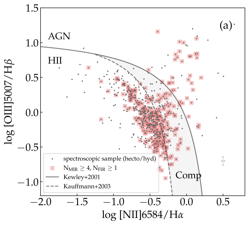
In order to use the metallicity estimators based on emission line ratios that are either empirically calibrated using star-forming galaxies or theoretically modeled for H ii regions, we exclude objects possibly dominated by active galactic nucleus (AGN) using a BPT diagram (Figure 2a) and a MIR color-color diagram (Figure 2b). In the BPT diagram, objects located below the AGN separation line (Kauffmann et al., 2003) are considered to be H ii galaxies, while the objects between the AGN line and the extreme starburst line (Kewley et al., 2001) are classified as composite systems (Kewley et al., 2006). Objects classified into three categories (H ii, composite, and AGN) in the BPT diagram (Figure 2a) are differently populated in MIR color-color diagram (Figure 2b), since MIR colors are affected by warm dusty torus around AGN. Almost, if not all, of the star-forming galaxies (“H ii”) are located outside the AGN selection wedge in the MIR color-color diagram. Note that only 25% of the AGN classified by optical spectral line ratios are located within the AGN selection window/wedge. This is explained by the fact that optical spectroscopic surveys are likely to be biased toward unobscured AGN, while MIR color-based AGN selection may identify highly obscured AGN. Completeness and reliability of AGN candidate selection are known to depend on the MIR color cut and magnitude (Assef et al., 2018). Considering MIR-selected AGN, the selection window/wedge in WISE color-color diagram is expected to be about 75% complete and fairly ($>80$%) reliable (Assef et al., 2018). Therefore, we use the selection window in the WISE color-color diagram to define photometrically selected AGN in case any of the four emission lines (H$\beta$, [O iii]$\lambda 5007$, H$\alpha$, and [N ii]$\lambda 6584$) is not detected. We exclude spectroscopically classified AGN/composite objects and photometrically selected AGN to construct the final sample of galaxies for metallicity measurement and SED fitting analysis.

The number of sample galaxies that satisfy (1) number of FIR (250, 350, and 500 $\mu$m) photometry, (2) number of MIR (7-24 $\mu$m) photometry, (3) H$\alpha$ and [N ii] line detection as well as $z_{\mathrm{spec}}<0.4$, and do not meet any of the AGN selection condition is 373. These galaxies are discussed in Section 5.

3 Metallicity Estimation

Figure 3: (a) Comparison between the oxygen abundance values derived using O3N2 index and N2 index (Pettini & Pagel, 2004). The uncertainties of $12+\mathrm{log(O/H)}$ implemented in two methods are 0.14 dex and 0.18 dex (at $1\sigma$) for O3N2 and N2, respectively. Such systematic uncertainty and uncertainty in the measured line flux ratio are quadratically summed to produce a typical error bar, marked in the corner. For Hii galaxies, $12+\mathrm{log(O/H)}$ values from O3N2 and N2 are consistent within 0.02. (b) Distribution of the $12+\mathrm{log(O/H)}$ values for spectroscopically observed objects (after the AGN exclusion), estimated using O3N2 index (371 objects) and N2 index (747 objects). Filled histograms are the metallicity distributions of objects satisfying criteria for availability of FIR and MIR photometric points (179 and 369 for O3N2 and N2 methods, respectively; the number of total objects with measured metallicity that meets other criteria is 373).

Among different metallicity indicators, one of the most widely used is the N2 index ($\mathrm{N2}\equiv\mathrm{log}{([\mathrm{N}\,\textsc{ii}]\lambda 6584/\mathrm{H}\alpha})$), while the ionization field strength that determines the observed nitrogen line flux is dependent on the gas-phase metallicity. In the low-metallicity (less than 20 % solar metallicity) and high-metallicity (above solar) regime, the higher-order polynomial fit is suggested to describe the relationship between N2 and $12+\mathrm{log(O/H)}$, rather than forcing a linear fit. Pettini & Pagel (2004) have suggested that the following equation is valid for extragalactic H ii regions in the range $-2.5<\mathrm{N2}<-0.3$, with $1\sigma$ uncertainty of 0.18 dex:

$$12+\mathrm{log(O/H)}=9.37+2.03\mathrm{N2}+1.26\mathrm{N2}^{2}+0.32\mathrm{N2}^{3}.$$ (1)

The merit of using the N2 index is that the uncertainty in extinction correction to derive this index is small since the [N ii]$\lambda 6584$ and H$\alpha$ lines are closely located in terms of the wavelength. The method is also applicable to the cases when no lines are detected in shorter wavelengths. However, in high-metallicity regime where [N ii] line saturates, adding [O iii] line is considered to provide better constraint on the metallicity as the [O iii] keeps decreasing with a decrease in oxygen abundance. An empirical calibration using [N ii]/H$\alpha$ and [O iii]/H$\beta$ line ratios, measured in the observed optical spectra, is known to be the O3N2 method. The O3N2 index is defined as $\mathrm{O3N2}\equiv\mathrm{log}$(([O iii]$\lambda 5007$/H$\beta$)/([N ii]$\lambda 6584$/H$\alpha$)). Based on the good linear correlation between the O3N2 and oxygen abundance of individual extragalactic H ii regions, the following conversion formula is suggested by Pettini & Pagel (2004, hereafter PP04 O3N2):

$$12+\mathrm{log(O/H)}=8.73-0.32\,\mathrm{O3N2}$$ (2)

of which $1\sigma$ systematic uncertainty is 0.14 dex. This equation is valid in the range $\mathrm{O3N2}<2$, corresponding to environments above 0.4 solar metallicity.

Since the uncertainty in the calibration formula is smaller in case of the O3N2 method than the N2 method, we use Equation 2 to derive gas-phase metallicity of sample galaxies. If [O iii] and/or H$\beta$ line are not detected in the optical spectrum (i.e., $\mathrm{S/N}<3$), Equation 1 is used instead. To derive line flux ratios, the measured line fluxes are corrected for dust attenuation using standard Milky Way reddening curve (Whitford, 1958) and the observed Balmer decrement H$\alpha$/H$\beta$ if both H$\alpha$ and H$\beta$ line fluxes are available. Recent work (Chartab et al., 2022) has warned that the use of rest-frame optical lines may underpredict the oxygen abundance for heavily obscured galaxies such as ultraluminous infrared galaxies (ULIRGs). Since the total IR luminosity of our sample galaxies is mostly $\mathrm{log}L_{\mathrm{IR}}[\mathrm{L}_{\odot}]<11.5$, none of our sample galaxies are classified as ULIRGs. The median of the extinction estimates, $\langle A_{V}\rangle$, of the sample galaxies are calculated to be 1.4 mag based on the H$\alpha$/H$\beta$ ratio. This value is comparable to that of local star-forming galaxies from SDSS (e.g., Hopkins et al., 2003), and is significantly smaller than $A_{V}(\mathrm{H}\alpha/\mathrm{H}\beta)\simeq 2.5$-2.9 mag of local ULIRGs and high-redshift submillimeter galaxies (e.g., Flores et al., 2004; Takata et al., 2006). Therefore we expect that it is appropriate to use the extinction-corrected optical line ratios in calculation of the oxygen abundance for our spectroscopic sample of MIR-selected galaxies.

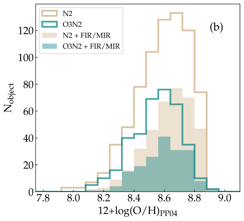
Figure 3a shows that the oxygen abundance values ($12+\mathrm{log(O/H)}$) derived using O3N2 and N2 are consistent with each other with a scatter of less than 0.02 dex in case of Hii galaxies. Objects for which metallicity is estimated using N2 index since O3N2 index is not available are more attenuated (about twice larger Balmer decrement) and slightly less luminous in H$\alpha$ (factor of 1.5 lower mean H$\alpha$ flux) compared to objects for which O3N2 index is available. Figure 3b shows the metallicity distribution of non-AGN objects. The metallicity of star-formation dominated galaxies ranges $7.9<12+\mathrm{log(O/H)}<9.0$, while the median metallicity is close to that of solar. If the sample criteria for FIR and MIR photometric data points are applied, the median metallicity for such galaxies is slightly higher. This suggests that our sample galaxies are likely to be affiliated in the massive galaxies among the entire MIR-selected galaxies, which is natural enough considering the FIR and MIR detection limits. As is already shown in Figure 1c, the final sample galaxies with MIR/FIR detection (marked in orrange) show slightly larger median stellar mass ($\langle\mathrm{log}\,M_{\mathrm{star}}[\mathrm{M}_{\odot}]\rangle=10.6$) and SFR ($\langle\mathrm{log}\,\mathrm{SFR}[\mathrm{M}_{\odot}\,\mathrm{yr}^{-1}]\rangle=0.3$) compared to entire spectroscopic sample. Therefore, our sample galaxies used in the investigation of metallicity-PAH relation are star-forming galaxies that lie above the median SFR of MIR-selected population. The SED fitting procedure to estimate physical parameters such as stellar mass and SFR is discussed in Section 4.

Figure 4: Example MIR-FIR SED of MIR-selected galaxies (best-fit template from cigale run). Blue solid and orange dashed lines represent (unattenuated) stellar component and dust emission component, respectively. Oxygen abundance $12+\mathrm{log(O/H)}$, PAH mass fraction derived from SED fitting, and redshift are indicated.

Table 1: Parameters for SED Fitting Using cigale

Model and Input parameters	Range
Star-formation history: sfhdelayed
e-folding time of the main stellar population model [Myr]	1000, 3000, 15000
Age of the main stellar population in the galaxy [Myr]	500, 2000, 5000, 6000, 7000, 8000, 9000, 10,000, 12,000
e-folding time of the late starburst population [Myr]	50
Age of the late starburst population [Myr]	20, 50, 100
Mass fraction of the late burst population	0.0, 0.1, 0.2, 0.3, 0.5
Stellar population: bc03
Initial mass function	Chabrier
Metallicity	0.02
Dust attenuation: dustatt_modified_CF00
Av_ISM	0.3, 0.6, 1.0, 1.6, 2.3, 3.8
Power-law slope of the attenuation in the ISM	$-$0.7
Power-law slope of the attenuation in the birth clouds	$-$1.3
Dust emission: dl2014
Mass fraction of PAH ($q_{\mathrm{PAH}}$)	0.47, 1.12, 1.77, 2.50, 3.19, 3.90, 4.58, 5.26, 5.95, 6.63, 7.32
Minimum radiation field ($U_{\mathrm{min}}$)	0.20, 1.00, 5.00, 10.00, 15.00, 25.00, 40.00
Power-law slope index ${\tilde{\alpha}}$ ($dU/dM\propto U^{\tilde{\alpha}}$)	1.6, 2.0, 2.3, 2.5, 2.7, 3.0
Fraction illuminated from $U_{\rm min}$ to $U_{\rm max}$ ($\gamma$)	0.00, 0.01, 0.02, 0.05, 0.1, 0.2, 0.3, 0.4, 0.5

Note that in Pettini & Pagel (2004), the number of high metallicity H ii regions ($12+\mathrm{log(O/H)}\simeq 9.0$, $\mathrm{O3N2}<0$) is small and oxygen abundances of such H ii regions are deduced from photoionization models rather than the electron temperature ($T_{e}$) method. Marino et al. (2013) have suggested a slightly flatter correlation between $12+\mathrm{log(O/H)}$ and O3N2 using the increased number of extragalactic H ii regions with $T_{e}$-based abundance measurements. The two calibrations agree with each other in low metallicity ranges, yet the difference between the two increases as the metallicity increases. For example, with $\mathrm{O3N2}=-1$, $12+\mathrm{log(O/H)}$ values calculated using Pettini & Pagel (2004) and Marino et al. (2013) are 9.0 and 8.7, respectively. The N2 methods suggested in Pettini & Pagel (2004) and Marino et al. (2013) have similar trend that Pettini & Pagel (2004) formula leads to higher metallicity than that of Marino et al. (2013). We use the N2 and O3N2 method of Pettini & Pagel (2004) in this study, and relatively metal-poor and metal-rich galaxies can be distinguished with a consistent manner. However, it should be noted that the derived $12+\mathrm{log(O/H)}$ values may not be the absolute oxygen abundance due to calibration uncertainty, and such uncertainty should be taken into account when comparing different works based on different methods.

4 SED Fitting

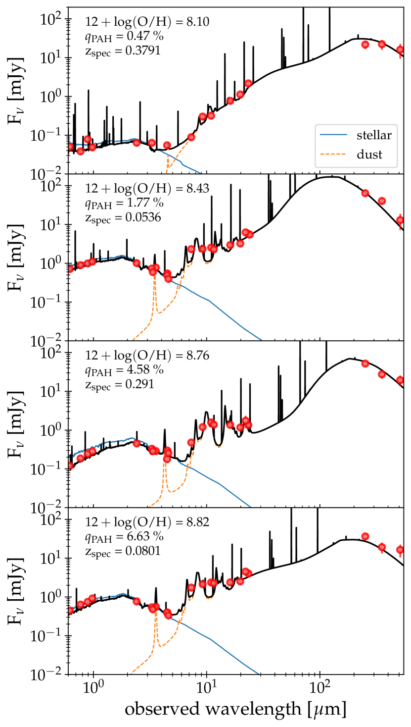
We fit the observed photometric points to the modeled SEDs using cigale (Code Investigating GAlaxy Emission, Noll et al., 2009; Boquien et al., 2019) to derive physical parameters of galaxies. The code cigale enables us to remove the stellar contribution from the observed SED by computing spectral template of a galaxy that consists of both stellar and dust component based on an energy balance principle, in which the energy from stars is reprocessed by dust to produce infrared emission. Stellar population synthesis model is convolved with the chosen star-formation history, which is then attenuated by dust. The computed spectral model (i.e., the sum of stellar component and dust emission component) is compared to the observed photometric points (or flux upper limits in case of nondetection) from UV to FIR wavelengths (0.1-500 $\mu$m). Figure 4 shows examples of best-fit templates with observed photometric data points for representative galaxies with different metallicity values (calculated in Section 3). The input parameters we use to run the modules of cigale are summarized in Table 1.

To calculate the stellar component, the “delayed” star-formation history model (sfhdelayed) is used. In this model, the SFR changes relatively smoothly according to the following formula:

$$\mathrm{SFR}(t)\propto\frac{t}{\tau^{2}}~{}\mathrm{exp}\left(-\frac{t}{\tau}\right),$$ (3)

which is valid at $0<t<t_{0}$, where $t_{0}$ is the time of star formation onset and $\tau$ is the time of SFR peak. By using small $\tau$ and large $\tau$, nearby passive galaxies and actively star-forming galaxies are efficiently modeled without the introduction of an abrupt, extreme change in SFR. For estimation of SFR and stellar mass, we choose to use the stellar population synthesis model of Bruzual & Charlot (2003) and Chabrier (2003) initial mass function. The stellar population metallicity is fixed to solar (0.02), since the relationship between oxygen abundance (gas metallicity) and stellar metallicity is not straightforward. The stellar component is reddened using the extended Charlot & Fall (2000) attenuation law, by allowing the attenuation $A_{V}$ to vary between 0.3 and 3.8 mag.

Figure 5: Test results to reproduce values of physical parameters based on the cigale run using mock catalog constructed from the best-fit SEDs. 373 non-AGN objects with estimated metallicity values are used to construct these plots. The $x$-axis represents the total IR luminosity, dust mass, mass fraction of PAH particles ($q_{\mathrm{PAH}}$), SFR, stellar mass, and IR excess (defined as the ratio between IR and UV luminosity) determined from the best-fit SED. A mock catalog is constructed using the expected flux density (based on the best-fit SED) and the observed flux uncertainty in each filter, which is to be used as an input in the cigale run with the same configuration to derive output ($y$-axis) value for each physical parameter. Gray dashed lines are $y=x$ lines, while the correlations between the input and output values are described as linear functions (blue solid lines) with the determination coefficients $r^{2}$. All properties are relatively well reproduced with strong correlation ($r^{2}>0.9$), supporting the robustness of the derived properties.

The key module to calculate the MIR-FIR SED is a dust emission module. cigale provides several ways of describing dust emission: semiempirical template (Dale et al., 2014); two-component model (Draine & Li, 2007; Draine et al., 2014); and the analytic model (Casey, 2012), as well as the model considering dust evolution according to local ISM physical condition (THEMIS; Jones et al., 2017). The dust templates of Dale et al. (2014) are constructed based on the modified SEDs of nearby star-forming galaxies with the addition of the AGN component; however, the model allows only limited variation in PAH emission. The Casey (2012) model consists of a single-temperature modified blackbody emission dominating FIR wavelengths and power-law continuum in MIR wavelengths, i.e., not taking PAH emission into account. The THEMIS model uses the fraction of HAC (hydrogenated amorphous carbons) as free parameter instead of PAH fraction, although the two are in general proportional to each other. Therefore, in order to estimate the PAH contribution in the SEDs of galaxies, we use the dl2014 module for modeling dust emission that is a refined version of the Draine & Li (2007) model.

In Draine & Li (2007) dust emission model, the spectral templates are calculated assuming that dust (silicate and graphite grains including various PAH particles) are heated by starlight. The starlight intensity $U$ (often characterized using minimum or maximum values, and the power-law slope $\tilde{\alpha}$ between them), the fraction of dust mass exposed to a starlight intensity distribution $\gamma$, and the PAH mass fraction $q_{\mathrm{PAH}}$ are free parameters for the spectral template calculation. Possible $q_{\mathrm{PAH}}$ values are [0.47, 1.12, 1.77, 2.50, 3.19, 3.90, 4.58] (%), which are tweaked to reproduce the Milky way extinction curve. Draine et al. (2014) have presented a slightly revised version of physical dust model of Draine & Li (2007), allowing a larger range of $q_{\mathrm{PAH}}$ – [0.47, 1.12, 1.77, 2.50, 3.19, 3.90, 4.58, 5.26, 5.95, 6.63, 7.32] – with slightly different normalization in total dust mass estimation. We use a wide range of $q_{\mathrm{PAH}}$, $U_{\mathrm{min}}$, $\tilde{\alpha}$, and $\gamma$ (Table 1) to reproduce diversities of MIR-FIR SED shape.

In addition to the modules and parameters in Table 1, we include nebular emission (nebular) and AGN (fritz2006) modules to compute models. However, nebular emission model parameters are fixed to default values (fixed ionization parameter, electron density and no Lyman continuum escape), and AGN module is practically switched off by fixing the AGN fraction to be zero. The reason for not considering the AGN component is because AGN-dominated galaxies, selected either spectroscopically or photometrically, are excluded from the sample (Figures 2a and 2b). To test whether such a strategy is reasonable, we fit SEDs of 179 spectroscopically selected H ii galaxies (for which O3N2 metallicity measurement is available) by switching the AGN module on, then compared best-fit models to that derived without the AGN component. The AGN component is calculated by varying AGN fraction (the ratio of AGN luminosity to total luminosity) to be between 0 and 1, with the range of 9.7 $\mu$m optical depth to be 0.6–6.0, and allowing opening angle between type 1 and type 2 AGN. For only two out of 179 (about 1 %) objects, the best-fit model is different, where the inclusion of the AGN component leads to a model with smaller $\chi^{2}$. The parameters associated with the AGN module indicate that these two prefer the AGN component contributing $\sim 10$ % of the total IR luminosity with a low optical depth of 9.7 $\mu$m silicate absorption. Considering the small number of such cases, the AGN fraction is assumed to be negligible in our sample of galaxies.

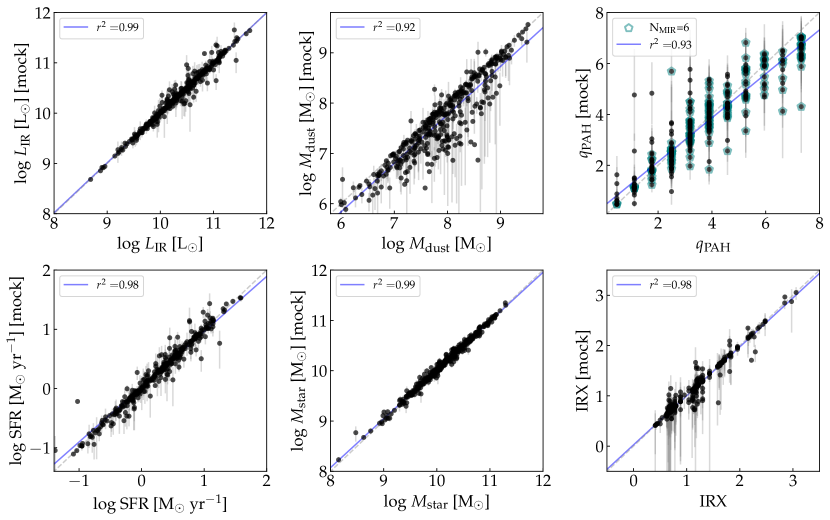
Physical properties of galaxies, such as the SFR, mass of the stellar and dust component, dust attenuation, dust luminosity (i.e., total IR luminosity), and PAH mass fraction are derived from the cigale run. Instead of extracting physical parameter values from the best-fit model, cigale probes the possible range for each parameter by taking the mean and standard deviation of the probability distribution function weighted for the goodness of fit. Such a strategy provides more robust estimates of properties and an idea of their uncertainties in case there exists degeneracy between physical properties. Based on this, it is also possible to investigate the reliability of the derived values of physical properties, through the “mock test” provided by cigale. In the mock test, once the best-fit SED model is determined for a galaxy, the synthetic flux density in each filter can be calculated from the best-fit model. By running the cigale again using the calculated synthetic flux densities and the observed flux uncertainties (i.e., mock catalog) with exactly the same configuration as the original run, it is possible to check whether the input physical values (values from the best-fit model) are well recovered, which allows us to assess the reliability of the derived values.

Figure 6: Correlation between different physical parameters: gas-phase metallicity $12+\mathrm{log(O/H)}$, stellar mass, specific SFR (sSFR), total IR luminosity, and mass fraction of PAH particles ($q_{\mathrm{PAH}}$). Spearman rank coefficients ($\rho$) between two variables in the $x$- and $y$-axis are specified in each panel. The sample is divided into three subsamples according to the redshift ($z<0.1$, $0.1\leq z<0.25$, and $0.25\leq z<0.4$), which results in a similar number of galaxies in each subsample. The distribution of each physical parameter is illustrated using a stacked histogram (in order of $0.25\leq z<0.4$, $0.1\leq z<0.25$, and $z<0.1$ bins) in order to better represent the difference between different subsamples.

The results of the mock test are summarized in Figure 5. Values for total IR luminosity, SFR, stellar mass, and IR excess (ratio between IR luminosity and UV luminosity) are robustly reproduced by a repeated cigale run that accounts for the observed flux uncertainties. In contrast to IR luminosity and stellar mass, the scatter between the input and output values is relatively large for the total dust mass and the PAH mass fraction. However, because the correlation coefficient is large enough ($r^{2}>0.9$), the relative comparison of $q_{\mathrm{PAH}}$ values between different galaxies is still valid. In panel for $q_{\mathrm{PAH}}$, galaxies that are detected in all six bands of the AKARI/IRC MIR wavelengths are separately marked. Although applying a criterion for number of MIR photometric points ($N_{\mathrm{MIR}}$) to be six removes some galaxies with large uncertainty in $q_{\mathrm{PAH}}$, it is not clear that the correlation coefficient becomes larger with $N_{\mathrm{MIR}}=6$ compared to the case of $N_{\mathrm{MIR}}\geq 4$. Therefore, the criterion is kept to be $N_{\mathrm{MIR}}\geq 4$ as mentioned in Section 2.4.

5 Results

Figure 7: (a) $q_{\mathrm{PAH}}$ vs. $12+\mathrm{log(O/H)}$ for 373 non-AGN MIR-selected galaxies (same plot as the panel (4,0) in Figure 6). Symbols are color-coded according to the sSFR. Typical error bar in oxygen abundance and $q_{\mathrm{PAH}}$ is marked in the corner. The mean value of the $q_{\mathrm{PAH}}$ is 2.3 and 3.7 for galaxies with $12+\mathrm{log(O/H)}<8.5$ and $12+\mathrm{log(O/H)}\geq 8.5$, respectively (horizontal lines). The black line is the linear regression describing the relationship between $12+\mathrm{log(O/H)}$ and $q_{\mathrm{PAH}}$, while gray lines are possibilities of linear correlation determined based on Bayesian methods considering uncertainties in $12+\mathrm{log(O/H)}$ and $q_{\mathrm{PAH}}$. (b) $q_{\mathrm{PAH}}$ vs. stellar mass. For galaxies in stellar mass bins of $\mathrm{log}(M_{\mathrm{star}}/\mathrm{M}_{\odot})=$[9.0, 9.5], [9.5, 10.0], [10.0, 10.5], and [10.5, 11.0], galaxies are divided into the low metallicity ($12+\mathrm{log(O/H)}<8.5$) and high metallicity ($12+\mathrm{log(O/H)}\geq 8.5$) subgroups and the mean $q_{\mathrm{PAH}}$ for each subgroup are plotted (note that points for the low metallicity subgroups are slightly shifted in $x$-direction for clarity). Overplotted are (1) $q_{\mathrm{PAH}}$ values measured from the stacked SEDs of $0.3<z<0.7$ star-forming galaxies in different stellar mass bins (black horizontal lines; Schreiber et al., 2018), and (2) $\langle q_{\mathrm{PAH}}\rangle$ values for different stellar mass bins of $z<0.7$ MIR/FIR-selected galaxies (gray horizontal lines; Kovács et al., 2019). The linear relationship between the $\mathrm{log}(M_{\mathrm{star}})$ and $q_{\mathrm{PAH}}$ and its posterior distribution is overplotted as black and gray lines.

5.1 Correlation between Physical Parameters

The typical values for physical properties of 373 MIR-selected non-AGN galaxies derived through SED fitting are as follows: stellar mass ranging $10^{8-11}\,\mathrm{M}_{\odot}$, having moderate ($\sim 0.1\,\mathrm{M}_{\odot}\,\mathrm{yr}^{-1}$) to large ($>10\,\mathrm{M}_{\odot}\,\mathrm{yr}^{-1}$) SFR represented by total IR luminosity of $10^{9-12}\,\mathrm{L}_{\odot}$.

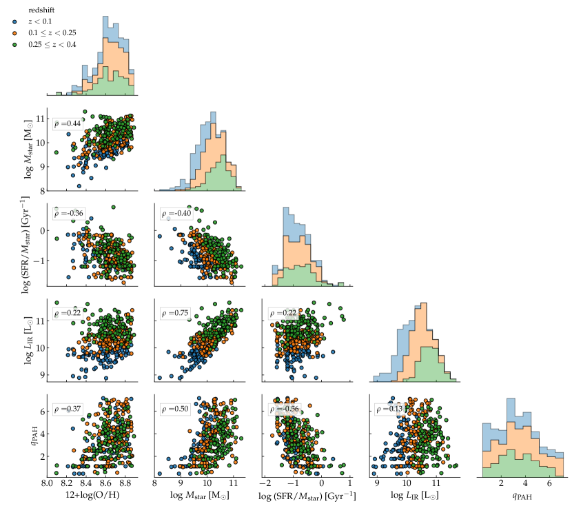
Figure 6 is a scatter plot matrix showing correlations between different physical parameters – $12+\mathrm{log(O/H)}$, stellar mass, specific SFR (sSFR; SFR divided by the stellar mass), total IR luminosity, and the PAH mass fraction, as well as the distribution of each parameter (in the diagonal locations). We present galaxies in different redshift bins with different colors. Number of galaxies in each redshift bin is 102, 158, and 113 for $z<0.1$, $0.1\leq z<0.25$, and $0.25\leq z<0.4$ bin, respectively. In case of stellar mass and IR luminosity, it is evident from the distribution plots that the properties are dependent on the redshift of galaxies. At higher redshifts, the MIR-selected sample consists of galaxies with larger median stellar mass and higher median IR luminosity. However, in case of $q_{\mathrm{PAH}}$ and $12+\mathrm{log(O/H)}$, the distributions look qualitatively similar even at different redshifts.

The Spearman’s rank correlation coefficients $\rho$ between $q_{\mathrm{PAH}}$ and other parameters are $0.37$, $0.50$, $-0.56$, and $0.13$ for $12+\mathrm{log(O/H)}$, $\mathrm{log}M_{\mathrm{star}}$, $\mathrm{log}(\mathrm{SFR}/M_{\mathrm{star}})$, and $\mathrm{log}L_{\mathrm{IR}}$. A positive correlation between $q_{\mathrm{PAH}}$ and gas-phase metallicity is found with $p$-value less than $10^{-5}$, suggesting that PAH features are on average weaker in lower metallicity galaxies than in higher metallicity galaxies. In addition, PAH mass fraction is positively correlated with stellar mass and negatively correlated with sSFR – that is, $q_{\mathrm{PAH}}$ is low in low-mass galaxies and in galaxies with large ongoing star-formation activity. The positive trend of increasing $q_{\mathrm{PAH}}$ as the increase of metallicity and stellar mass reflects the mass-metallicity relation (e.g., Tremonti et al., 2004), which is also observed with $\rho=0.44$ in our sample. Although a mass-SFR correlation of star-forming galaxies is present as is seen in the $\mathrm{log}L_{\mathrm{IR}}$ versus $\mathrm{log}M_{\mathrm{star}}$ plot (with $\rho=0.75$), the dependence of $q_{\mathrm{PAH}}$ on the IR luminosity is relatively weak unlike the other physical parameters.

5.2 Metallicity and $q_{\mathrm{PAH}}$ Variation

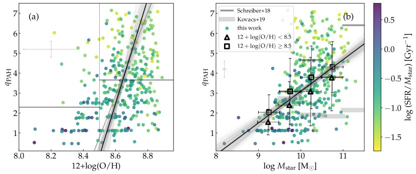
Based on Figure 6, $q_{\mathrm{PAH}}$ is positively correlated with both metallicity and stellar mass. In Figures 7a and 7b, we show the linear regression results between dependent variable $q_{\mathrm{PAH}}$ and independent variables metallicity and stellar mass. When performing linear regression, the uncertainties in the derived $12+\mathrm{log(O/H)}$, stellar mass, and $q_{\mathrm{PAH}}$ are taken into account using a Bayesian approach (Kelly, 2007). The principle of the method described in Kelly (2007) is that with measurement errors in $x$ and $y$, linear regression is performed for new independent ($\xi$) and dependent ($\eta$) variables that are defined as $x_{i}\equiv\xi_{i}+\mathrm{error}(x_{i})$ and $y_{i}\equiv\eta_{i}+\mathrm{error}(y_{i})$. By applying the MCMC algorithm, the posterior distribution of the regression coefficients are derived, along with the Pearson linear coefficient for ($x,y$). Since the uncertainties in the $12+\mathrm{log(O/H)}$ are much larger than those in the stellar mass, the linear correlation coefficient for $q_{\mathrm{PAH}}$-metallicity relation ($0.97\pm 0.03$) is higher than that of the $q_{\mathrm{PAH}}$-stellar mass relation ($0.52\pm 0.04$). In addition, the $q_{\mathrm{PAH}}$ values for our sample galaxies are compared to results from previous works (Schreiber et al., 2018; Kovács et al., 2019), which presented $q_{\mathrm{PAH}}$ according to stellar mass (Figure 7b). Although our sample consists of less massive galaxies than those studied in previous works, $q_{\mathrm{PAH}}$ values are similar in the stellar mass range that overlaps with that of Schreiber et al. (2018). The black lines in Figures 7a and b are as follows:

$$q_{\mathrm{PAH}}=(-240.5\pm 45.5)+(28.3\pm 5.3)(\mathrm{12+log(O/H)}),$$ (4)

$$q_{\mathrm{PAH}}=(-12.8\pm 1.5)+(1.6\pm 0.2)~{}\mathrm{log}\,M_{\mathrm{star}}[\mathrm{M}_{\odot}].$$ (5)

In order to investigate the variation of PAH strength in terms of metallicity, in a situation where other physical parameters such as stellar mass is fixed, the galaxies are divided into low-metallicity and high-metallicity groups using a divider of $12+\mathrm{log(O/H)}=8.5$. The value corresponds to $\sim 0.5\,Z_{\odot}$ if solar oxygen abundance is assumed to be $12+\mathrm{log(O/H)}=8.73$ (Asplund et al., 2009). Figure 7a shows that the mean $q_{\mathrm{PAH}}$ value of the low-metallicity group (2.3%) is lower than that of the high-metallicity group (3.7%). This is in line with the result presented in Ciesla et al. (2014), that metallicity and PAH fraction are directly linked in local gas-rich galaxies. In Figure 7b, $\langle q_{\mathrm{PAH}}\rangle$ values for the different metallicity group of galaxies in each stellar mass bin (with step size $\Delta\mathrm{log}(M_{\mathrm{star}}/\mathrm{M}_{\odot})=0.5$) are shown as different symbols. In the stellar mass range of $\mathrm{log}(M_{\mathrm{star}}/\mathrm{M}_{\odot})=[9,11]$, $\langle q_{\mathrm{PAH}}\rangle$ values of galaxies in the higher metallicity group are always higher than that of galaxies in the lower metallicity group. Therefore, it can be concluded that the PAH features are correlated with metallicity, even if the stellar mass is fixed, when only two variables (metallicity and stellar mass) are considered.

Figure 8: (a) Comparison between $q_{\mathrm{PAH}}$ derived from SED fitting and luminosity ($\nu L_{\nu}$) ratio between 8 $\mu$m and 4.5 $\mu$m – the former stands for PAH emission and the latter for stellar continuum (Murata et al., 2014). Blue solid line is the best-fit linear correlation with specified determination coefficient $r^{2}$. (b) Comparison between $q_{\mathrm{PAH}}$ and IR8, defined as $L_{\mathrm{IR}}^{\mathrm{total}}/\nu L_{\nu}(8\mu\mathrm{m})$. Overplotted curve is the correlation between the two suggested by Schreiber et al. (2018). (c) Comparison between luminosity fraction of PAH features (relative to total IR emission) and mass fraction $q_{\mathrm{PAH}}$. PAH luminosity is calculated by the sum of luminosities of 6.2 $\mu$m and 7.7 $\mu$m features from Ohyama et al. (2018).

From Figure 6, it is clear that sSFR is strongly correlated with the $q_{\mathrm{PAH}}$, showing an even larger correlation coefficient than that in case of stellar mass and metallicity. The correlation also is in line with stellar mass-SFR relation composed of galaxies in the star-forming main sequence. With symbol colors coded according to sSFR in Figures 7a and 7b, the three parameters (metallicity, stellar mass, and sSFR) seem to be correlated with each other. In order to understand which is the primary correlation that drives $q_{\mathrm{PAH}}$ variation, we calculate the partial correlation coefficients between $q_{\mathrm{PAH}}$ and each parameter while the effects of the other two parameters are removed. The results are $0.10$, $0.32$, and $-0.43$ in case of $12+\mathrm{log(O/H)}$, $\mathrm{log}M_{\mathrm{star}}$, and $\mathrm{log}\,\mathrm{sSFR}$. This corresponds to $p$-values of 0.067, $<10^{-5}$, and $<10^{-5}$. All three parameters are correlated to $q_{\mathrm{PAH}}$ even when effects of other parameters are removed, and among these three, sSFR appears to be the most strongly correlated parameter. However, considering the fact that coefficient calculation is affected by uncertainties as is mentioned above, it is still difficult to make a firm conclusion. The existence and the effectiveness of metallicity-mass-SFR correlation or so-called fundamental plane of star-forming galaxies is still being debated (e.g., Lara-López et al., 2010; Sánchez et al., 2017). At least for our sample of MIR-selected galaxies, metallicity-mass-SFR correlation does exist and affects PAH strength.

5.3 $q_{\mathrm{PAH}}$ Estimators

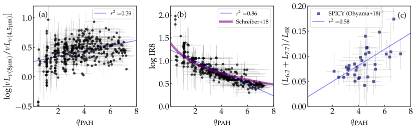
Using the MIR-selected star-forming galaxies sample, we compare observable luminosity ratios suggested by previous studies to $q_{\mathrm{PAH}}$ parameters derived from SED fitting. For example, Murata et al. (2014) have suggested 8 $\mu$m-to-4.5 $\mu$m luminosity ratio traces PAH emission features, since rest-frame 8 $\mu$m luminosity is mainly from PAH emission and 4.5 $\mu$m luminosity represents stellar continuum in case of non-AGN galaxies. They have shown that $\nu L_{\nu}(8\,\mu\mathrm{m})/\nu L_{\nu}(4.5\,\mu\mathrm{m})$ increases with “starburstiness,” i.e., offset from the star-forming main sequence, yet the ratio saturates above a certain limit. We show in Figure 8a, how $\nu L_{\nu}(8\,\mu\mathrm{m})/\nu L_{\nu}(4.5\,\mu\mathrm{m})$ differs as a function of $q_{\mathrm{PAH}}$. Little correlation is found between $q_{\mathrm{PAH}}$ and $\nu L_{\nu}(8\mu\mathrm{m})/\nu L_{\nu}(4.5\mu\mathrm{m})$, suggesting that although the ratio between 8-$\mu$m and 4.5-$\mu$m luminosity may give insight to the existence of PAH emission features, it is difficult to estimate the relative strength of PAH emission compared to the total dust emission.

On the other hand, the IR8 value ($\mathrm{IR8}\equiv L_{\mathrm{IR}}/\nu L_{\nu}(8\mu\mathrm{m})$, Elbaz et al., 2011) is well correlated with the $q_{\mathrm{PAH}}$ (Figure 8b). The correlation between IR8 and $q_{\mathrm{PAH}}$ used in generating a wide range of IR SEDs in Schreiber et al. (2018) is consistent with our sample of galaxies.

Finally, we show the relative luminosity ratio between PAH and total IR luminosity versus PAH mass fraction in Figure 8c, using sources for which 5-13 $\mu$m spectra have been obtained (Ohyama et al., 2018). The ratio between PAH luminosity estimated from specific features (rest frame 6.2 and 7.7 $\mu$m) and total IR luminosity is positively correlated with $q_{\mathrm{PAH}}$. However, scatters imply that variation between the PAH features at different wavelengths might be nonnegligible in estimating $q_{\mathrm{PAH}}$.

Figure 9: (a) Molecular gas mass for MIR-selected galaxies as a function of stellar mass. In order to calculate the molecular gas mass ($M_{\mathrm{H}_{2}}$), total gas mass is estimated using $\delta_{\mathrm{GDR}}$-metallicity calibration (De Vis et al., 2019), dust mass from SED fitting, and metallicity-dependent H₂/Hi mass ratio (Boselli et al., 2014). Error bar in the left corner represents typical uncertainties in the derived $M_{\mathrm{H}_{2}}$. Overplotted symbols are $0.05<z<0.5$ star-forming galaxies with measured molecular gas mass through CO observations (squares and triangles; Bauermeister et al., 2013; Villanueva et al., 2017). Linear regression fit between the gas mass and stellar mass of our sample galaxies is plotted as a thick black line, along with thin gray lines covering a possible range of linear relation. (b) Gas depletion time ($M_{\mathrm{gas}}/\mathrm{SFR}$) vs. sSFR ($\mathrm{SFR}/M_{\mathrm{star}}$) for our sample of MIR-selected galaxies. Error bar in the corner represents typical uncertainties in $x$- and $y$-axis parameters, reflecting the estimation errors as well as scatter in a conversion formula. Again, the CO-detected samples from Bauermeister et al. (2013) and Villanueva et al. (2017) are plotted for comparison. The thick black line and thin gray lines show linear regression results. Dot-dashed and dashed lines indicate depletion time vs. sSFR relation for nearby ($z<0.05$) galaxies measured either using global gas mass (COLD GASS; Saintonge et al., 2011; Huang & Kauffmann, 2014) or gas mass derived for 1 kpc grids (HERACLES; Huang & Kauffmann, 2014). Dotted line is such a relation for local (with distance $<25$ Mpc) ‘gas-rich’ galaxies among the Herschel reference survey galaxies (Boselli et al., 2014).

5.4 Dust Mass as a Tracer of Gas Mass

It is suggested that total dust mass ($M_{\mathrm{dust}}$) in a galaxy can be used as a proxy for estimating gas mass (e.g., Groves et al., 2015; Berta et al., 2016), since the gas and dust content of galaxies are linked to each other through a gas-to-dust mass ratio ($\delta_{\mathrm{GDR}}$). The gas-to-dust ratio is found to be a function of metallicity, in a way that gas-to-dust ratio decreases as the metallicity increases (Leroy et al., 2011; Magdis et al., 2012; Rémy-Ruyer et al., 2014; De Vis et al., 2019). For our MIR-selected star-forming galaxies at $z<0.4$, we combine the metallicity-dependent gas-to-dust ratio ($\delta_{\mathrm{GDR}}$) with the dust mass ($M_{\mathrm{dust}}$) to estimate the gas mass in these galaxies ($M_{\mathrm{gas}}\equiv\delta_{\mathrm{GDR}}M_{\mathrm{dust}}$). Dust masses are estimated from the SED fitting (Section 4) using the dust emission model of Draine et al. (2007). For gas-to-dust ratio, we use the following $\delta_{\mathrm{GDR}}$-metallicity calibration from De Vis et al. (2019):

$$\mathrm{log}\delta_{\mathrm{GDR}}=(21.19\pm 0.90)-(2.15\pm 0.11)(12+\mathrm{log(O/H)}).$$ (6)

The formula is calibrated using Dustpedia data sets that consist of nearby ($v<3000$ km s^-1) extended galaxies with Herschel FIR observations. Differences in the dust emission models used in De Vis et al. (2019) (THEMIS; Nersesian et al., 2019) and our work (Draine et al., 2007) are taken into account (for systematics and uncertainties of measuring dust mass based on different methods of modeling FIR dust emission, see Berta et al. 2016). In our case, using the Draine et al. (2007) model leads to a factor of 1.5 higher dust mass compared to the case of using THEMIS model. The gas mass in the calibration formula corresponds to the ‘total’ gas mass, including molecular hydrogen and atomic hydrogen, as well as gas of heavier elements ($M_{\mathrm{gas}}=\xi M_{\mathrm{H\textsc{i}}}(1+M_{\mathrm{H_{2}}}/M_{\mathrm{H\textsc{i}}})$, De Vis et al., 2019). Therefore, in order to compare our results with CO observations of star-forming galaxies at similar redshift range, we calculate molecular hydrogen mass by applying $\xi=1.39$ and $M_{\mathrm{H_{2}}}/M_{\mathrm{H\textsc{i}}}$ ratio that is dependent on the oxygen abundance (Boselli et al., 2014). In our oxygen abundance range, the $M_{\mathrm{H_{2}}}/M_{\mathrm{H\textsc{i}}}$ varies in the range of 0.1 to 0.8.

Figure 9a shows that our MIR-selected galaxies have molecular hydrogen gas mass of the range of $\mathrm{log}\,M_{\mathrm{H_{2}}}[\mathrm{M}_{\odot}]=7.5$-11.5. Spearman rank coefficient between $\mathrm{log}\,M_{\mathrm{H2}}$ and $\mathrm{log}\,M_{\mathrm{star}}$ is $0.60$, and if the errors in two parameters are taken into account, the Pearson correlation coefficient is $0.91\pm 0.04$. The linear regression suggests following correlation between the stellar and dust mass:

$$\mathrm{log}\,M_{\mathrm{H_{2}}}[\mathrm{M}_{\odot}]=(-0.49\pm 0.63)+(0.96\pm 0.06)~{}\mathrm{log}\,M_{\mathrm{star}}[\mathrm{M}_{\odot}].$$ (7)

Compared in Figure 9a are star-forming galaxies at similar redshift range ($0.05<z<0.5$; Bauermeister et al., 2013; Villanueva et al., 2017), of which gas masses are estimated from CO observations. Galaxies from Bauermeister et al. (2013) (squares in Figure 9a) are selected based on the large SFR (of order of several tens $\mathrm{M}_{\odot}\,\mathrm{yr}^{-1}$) with a stellar mass of order of $10^{10.6-11.5}\,\mathrm{M}_{\odot}$, thus are galaxies above the star-forming galaxy main sequence in SFR-stellar mass plane, sharing similar positions with local LIRGs. Galaxies from Villanueva et al. (2017) (triangles in Figure 9a) are galaxies selected in the 160 $\mu$m, of which total IR luminosity is larger than $10^{11}\,\mathrm{L}_{\odot}$ in most cases. Therefore the compared $0.05<z<0.5$ galaxies with CO detections are ‘scaled-up’ versions of our MIR-selected galaxies with an order of larger average stellar mass and an order of larger SFR. The fact that CO-detected galaxies show similar $M_{\mathrm{H_{2}}}$-$M_{\mathrm{star}}$ correlation with our sample implies that the gas-to-star mass fraction is roughly consistent in a wide stellar mass range of $10^{9}$-$10^{11}$ M_⊙.

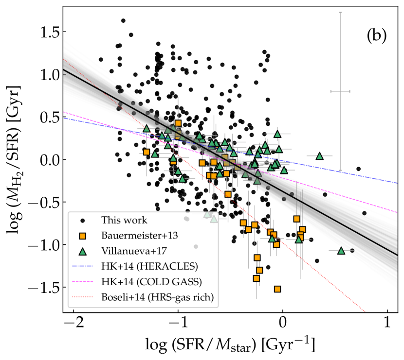
In Figure 9b, we show the molecular gas depletion time ($\tau_{\mathrm{dep}}\equiv M_{\mathrm{H_{2}}}/\mathrm{SFR}$) of our sample galaxies as a function of sSFR. From the CO-detected galaxies (Bauermeister et al., 2013; Villanueva et al., 2017), it is noticeable that the gas depletion time scale has a negative correlation with the sSFR. Such a trend is also observed for nearby ($z<0.05$) galaxies (see dashed, dotted-dashed, and dotted lines in Figure 9b; Huang & Kauffmann, 2014; Boselli et al., 2014), and implies that a fast consumption of gas in starburst galaxies is present throughout to $z\sim 0.5$. Although the uncertainties in gas mass (and thus $\tau_{\mathrm{dep}}$) is very large, we derive the following relation between $\tau_{\mathrm{dep}}$ and sSFR through linear regression:

$$\mathrm{log\,\tau_{\mathrm{dep}}}[\mathrm{Gyr}]=(-0.38\pm 0.06)+(-0.68\pm 0.07)~{}\mathrm{log\,sSFR}[\mathrm{Gyr}^{-1}].$$ (8)

Note that Spearman rank coefficient between two parameters is $-0.45$, while the linear correlation coefficient estimated with the consideration of the parameter uncertainties is $-0.88\pm 0.07$. Like local and low-redshift galaxies with CO detection, MIR-selected galaxies are suspected to have shorter gas depletion time scales if the sSFR are larger. Boselli et al. (2014) have suggested that the slope of the $\tau_{\mathrm{dep}}$-sSFR relation is steeper if only gas-rich, late type galaxies are considered, compared to the case when all galaxies (targets of CO observation with only upper limits, i.e., nondetections, like in the case of Huang & Kauffmann (2014)) are used to derive the correlation. The $\tau_{\mathrm{dep}}$-sSFR relation of our MIR-selected sample galaxies suggests that MIR-selected galaxies are similar to gas-rich galaxies.

6 Summary

Based on the optical spectra and the multiwavelength photometry, we estimate gas-phase metallicity and physical parameters of MIR-selected galaxies at $z<0.4$. The motivation of this work is to utilize multiple broad-band photometric information in MIR wavelengths to constrain relative strength of PAH emission, which is a key to understanding the scatter in ratio between the MIR and total IR luminosity. The total IR luminosity as well as the mass fraction of PAH particles among total dust mass are estimated through SED fitting.

The PAH mass fraction $q_{\mathrm{PAH}}$ is dependent on the gas-phase metallicity measured using strong emission lines, i.e., $q_{\mathrm{PAH}}$ increases as the metallicity increases. The result is in line with previous studies using local star-forming galaxies. Since possible AGN contaminants are excluded from the sample based on optical line ratios and MIR colors, the result shows that characteristics of low metallicity ISM environments for pure H ii galaxies suppress the PAH emission. Suggestions have been made that a harder UV-radiation field (originating from less dust shielding) in a low-metallicity environment is effective in the destruction of PAH particles. The $q_{\mathrm{PAH}}$ value is also dependent on the stellar mass and sSFR, in a way that PAH features are weaker in less massive galaxies and in galaxies where current SFR is relatively larger compared to the accumulated stellar mass. Partial correlation coefficients between $q_{\mathrm{PAH}}$ and physical parameters suggest that $q_{\mathrm{PAH}}$ value of galaxies with similar stellar mass and sSFR is still a function of metallicity, while the same trend is found for the cases of stellar mass and sSFR. This reflects the mass-metallicity relation of galaxies, as well as implying the mass-metallicity-SFR scaling relation of star-forming galaxies.

The metallicity of galaxies not only affects the PAH strength that dominates MIR wavelengths, but also provides a link between gas and dust mass in galaxies. Applying metallicity-dependent gas-to-dust ratio calibration to our sample galaxies, a trend of decreasing gas depletion time scale along the increase of sSFR is reproduced, similarly to the case of CO-observed galaxies. Considering these, metallicity is one of the main factors that is necessary to describe the variation in MIR-FIR SED.

References

- Alonso-Herrero et al. (2020) Alonso-Herrero, A., Pereira-Santaella, M., Rigopoulou, D., et al. 2020, A&A, 639, A43. doi:10.1051/0004-6361/202037642
- Asplund et al. (2009) Asplund, M., Grevesse, N., Sauval, A. J., et al. 2009, ARA&A, 47, 481. doi:10.1146/annurev.astro.46.060407.145222
- Assef et al. (2018) Assef, R. J., Stern, D., Noirot, G., et al. 2018, ApJS, 234, 23. doi:10.3847/1538-4365/aaa00a
- Bianchi et al. (2017) Bianchi, L., Shiao, B., & Thilker, D. 2017, ApJS, 230, 24. doi:10.3847/1538-4365/aa7053
- Baldwin et al. (1981) Baldwin, J. A., Phillips, M. M., & Terlevich, R. 1981, PASP, 93, 5. doi:10.1086/130766
- Bauermeister et al. (2013) Bauermeister, A., Blitz, L., Bolatto, A., et al. 2013, ApJ, 768, 132. doi:10.1088/0004-637X/768/2/132
- Berta et al. (2016) Berta, S., Lutz, D., Genzel, R., et al. 2016, A&A, 587, A73. doi:10.1051/0004-6361/201527746
- Boquien et al. (2019) Boquien, M., Burgarella, D., Roehlly, Y., et al. 2019, A&A, 622, A103. doi:10.1051/0004-6361/201834156
- Boselli et al. (2014) Boselli, A., Cortese, L., Boquien, M., et al. 2014, A&A, 564, A66. doi:10.1051/0004-6361/201322312
- Bruzual & Charlot (2003) Bruzual, G. & Charlot, S. 2003, MNRAS, 344, 1000. doi:10.1046/j.1365-8711.2003.06897.x
- Calzetti et al. (2007) Calzetti, D., Kennicutt, R. C., Engelbracht, C. W., et al. 2007, ApJ, 666, 870. doi:10.1086/520082
- Casey (2012) Casey, C. M. 2012, MNRAS, 425, 3094. doi:10.1111/j.1365-2966.2012.21455.x
- Chabrier (2003) Chabrier, G. 2003, PASP, 115, 763. doi:10.1086/376392
- Charlot & Fall (2000) Charlot, S. & Fall, S. M. 2000, ApJ, 539, 718. doi:10.1086/309250
- Chartab et al. (2022) Chartab, N., Cooray, A., Ma, J., et al. 2022, Nature Astronomy, 6, 844. doi:10.1038/s41550-022-01679-y
- Ciesla et al. (2014) Ciesla, L., Boquien, M., Boselli, A., et al. 2014, A&A, 565, A128. doi:10.1051/0004-6361/201323248
- Cutri et al. (2012) Cutri, R. M. & et al. 2012, VizieR Online Data Catalog, II/311
- Dale et al. (2014) Dale, D. A., Helou, G., Magdis, G. E., et al. 2014, ApJ, 784, 83. doi:10.1088/0004-637X/784/1/83
- Desai et al. (2006) Desai, V., Armus, L., Soifer, B. T., et al. 2006, ApJ, 641, 133. doi:10.1086/500426
- De Vis et al. (2019) De Vis, P., Jones, A., Viaene, S., et al. 2019, A&A, 623, A5. doi:10.1051/0004-6361/201834444
- Draine & Li (2007) Draine, B. T. & Li, A. 2007, ApJ, 657, 810. doi:10.1086/511055
- Draine et al. (2007) Draine, B. T., Dale, D. A., Bendo, G., et al. 2007, ApJ, 663, 866. doi:10.1086/518306
- Draine et al. (2014) Draine, B. T., Aniano, G., Krause, O., et al. 2014, ApJ, 780, 172. doi:10.1088/0004-637X/780/2/172
- Dwek (2005) Dwek, E. 2005, The Spectral Energy Distributions of Gas-Rich Galaxies: Confronting Models with Data, 761, 103. doi:10.1063/1.1913921
- Elbaz et al. (2005) Elbaz, D., Le Floc’h, E., Dole, H., et al. 2005, A&A, 434, L1. doi:10.1051/0004-6361:200500095
- Elbaz et al. (2011) Elbaz, D., Dickinson, M., Hwang, H. S., et al. 2011, A&A, 533, A119. doi:10.1051/0004-6361/201117239
- Engelbracht et al. (2005) Engelbracht, C. W., Gordon, K. D., Rieke, G. H., et al. 2005, ApJ, 628, L29. doi:10.1086/432613
- Flores et al. (2004) Flores, H., Hammer, F., Elbaz, D., et al. 2004, A&A, 415, 885. doi:10.1051/0004-6361:20034491
- Jeon et al. (2014) Jeon, Y., Im, M., Kang, E., et al. 2014, ApJS, 214, 20. doi:10.1088/0067-0049/214/2/20
- Galliano et al. (2008) Galliano, F., Dwek, E., & Chanial, P. 2008, ApJ, 672, 214. doi:10.1086/523621
- Galliano et al. (2008) Galliano, F., Madden, S. C., Tielens, A. G. G. M., et al. 2008, ApJ, 679, 310. doi:10.1086/587051
- Goto et al. (2010) Goto, T., Takagi, T., Matsuhara, H., et al. 2010, A&A, 514, A6. doi:10.1051/0004-6361/200913182
- Groves et al. (2015) Groves, B. A., Schinnerer, E., Leroy, A., et al. 2015, ApJ, 799, 96. doi:10.1088/0004-637X/799/1/96
- Ho et al. (2021) Ho, S. C.-C., Goto, T., Oi, N., et al. 2021, MNRAS, 502, 140. doi:10.1093/mnras/staa3549
- Hopkins et al. (2003) Hopkins, A. M., Miller, C. J., Nichol, R. C., et al. 2003, ApJ, 599, 971. doi:10.1086/379608
- Huang & Kauffmann (2014) Huang, M.-L. & Kauffmann, G. 2014, MNRAS, 443, 1329. doi:10.1093/mnras/stu1232
- Huang et al. (2020) Huang, T.-C., Matsuhara, H., Goto, T., et al. 2020, MNRAS, 498, 609. doi:10.1093/mnras/staa2459
- Hurley et al. (2017) Hurley, P. D., Oliver, S., Betancourt, M., et al. 2017, MNRAS, 464, 885. doi:10.1093/mnras/stw2375
- Hwang et al. (2007) Hwang, N., Lee, M. G., Lee, H. M., et al. 2007, ApJS, 172, 583. doi:10.1086/519216
- Jarrett et al. (2011) Jarrett, T. H., Cohen, M., Masci, F., et al. 2011, ApJ, 735, 112. doi:10.1088/0004-637X/735/2/112
- Jones et al. (2017) Jones, A. P., Köhler, M., Ysard, N., et al. 2017, A&A, 602, A46. doi:10.1051/0004-6361/201630225
- Kauffmann et al. (2003) Kauffmann, G., Heckman, T. M., Tremonti, C., et al. 2003, MNRAS, 346, 1055. doi:10.1111/j.1365-2966.2003.07154.x
- Kelly (2007) Kelly, B. C. 2007, ApJ, 665, 1489. doi:10.1086/519947
- Kennicutt et al. (2003) Kennicutt, R. C., Armus, L., Bendo, G., et al. 2003, PASP, 115, 928. doi:10.1086/376941
- Kewley et al. (2001) Kewley, L. J., Dopita, M. A., Sutherland, R. S., et al. 2001, ApJ, 556, 121. doi:10.1086/321545
- Kewley et al. (2006) Kewley, L. J., Groves, B., Kauffmann, G., et al. 2006, MNRAS, 372, 961. doi:10.1111/j.1365-2966.2006.10859.x
- Kim et al. (2012) Kim, S. J., Lee, H. M., Matsuhara, H., et al. 2012, A&A, 548, A29. doi:10.1051/0004-6361/201219105
- Kim et al. (2021) Kim, S. J., Oi, N., Goto, T., et al. 2021, MNRAS, 500, 4078. doi:10.1093/mnras/staa3359
- Knight et al. (2022) Knight, C., Peeters, E., Tielens, A. G. G. M., et al. 2022, MNRAS, 509, 3523. doi:10.1093/mnras/stab3047
- Kovács et al. (2019) Kovács, T. O., Burgarella, D., Kaneda, H., et al. 2019, PASJ, 71, 27. doi:10.1093/pasj/psy145
- Lagache et al. (2004) Lagache, G., Dole, H., Puget, J.-L., et al. 2004, ApJS, 154, 112. doi:10.1086/422392
- Lai et al. (2020) Lai, T. S.-Y., Smith, J. D. T., Baba, S., et al. 2020, ApJ, 905, 55. doi:10.3847/1538-4357/abc002
- Lara-López et al. (2010) Lara-López, M. A., Cepa, J., Bongiovanni, A., et al. 2010, A&A, 521, L53. doi:10.1051/0004-6361/201014803
- Lee et al. (2012) Lee, J. C., Hwang, H. S., Lee, M. G., et al. 2012, ApJ, 756, 95. doi:10.1088/0004-637X/756/1/95
- Leroy et al. (2011) Leroy, A. K., Bolatto, A., Gordon, K., et al. 2011, ApJ, 737, 12. doi:10.1088/0004-637X/737/1/12
- Li (2020) Li, A. 2020, Nature Astronomy, 4, 339. doi:10.1038/s41550-020-1051-1
- Lutz et al. (2005) Lutz, D., Valiante, E., Sturm, E., et al. 2005, ApJ, 625, L83. doi:10.1086/431217
- Madden et al. (2006) Madden, S. C., Galliano, F., Jones, A. P., et al. 2006, A&A, 446, 877. doi:10.1051/0004-6361:20053890
- Magdis et al. (2012) Magdis, G. E., Daddi, E., Béthermin, M., et al. 2012, ApJ, 760, 6. doi:10.1088/0004-637X/760/1/6
- Maragkoudakis et al. (2018) Maragkoudakis, A., Ivkovich, N., Peeters, E., et al. 2018, MNRAS, 481, 5370. doi:10.1093/mnras/sty2658
- Maragkoudakis et al. (2020) Maragkoudakis, A., Peeters, E., & Ricca, A. 2020, MNRAS, 494, 642. doi:10.1093/mnras/staa681
- Marino et al. (2013) Marino, R. A., Rosales-Ortega, F. F., Sánchez, S. F., et al. 2013, A&A, 559, A114. doi:10.1051/0004-6361/201321956
- Markwardt (2009) Markwardt, C. B. 2009, Astronomical Data Analysis Software and Systems XVIII, 411, 251
- Mateos et al. (2012) Mateos, S., Alonso-Herrero, A., Carrera, F. J., et al. 2012, MNRAS, 426, 3271. doi:10.1111/j.1365-2966.2012.21843.x
- Murakami et al. (2007) Murakami, H., Baba, H., Barthel, P., et al. 2007, PASJ, 59, S369. doi:10.1093/pasj/59.sp2.S369
- Murata et al. (2014) Murata, K., Matsuhara, H., Inami, H., et al. 2014, A&A, 566, A136. doi:10.1051/0004-6361/201423744
- Murata et al. (2017) Murata, K. L., Yamada, R., Oyabu, S., et al. 2017, MNRAS, 472, 39. doi:10.1093/mnras/stx1902
- Nayyeri et al. (2018) Nayyeri, H., Ghotbi, N., Cooray, A., et al. 2018, ApJS, 234, 38. doi:10.3847/1538-4365/aaa07e
- Nersesian et al. (2019) Nersesian, A., Xilouris, E. M., Bianchi, S., et al. 2019, A&A, 624, A80. doi:10.1051/0004-6361/201935118
- Nguyen et al. (2010) Nguyen, H. T., Schulz, B., Levenson, L., et al. 2010, A&A, 518, L5. doi:10.1051/0004-6361/201014680
- Noll et al. (2009) Noll, S., Burgarella, D., Giovannoli, E., et al. 2009, A&A, 507, 1793. doi:10.1051/0004-6361/200912497
- Oi et al. (2021) Oi, N., Goto, T., Matsuhara, H., et al. 2021, MNRAS, 500, 5024. doi:10.1093/mnras/staa3080
- Ohyama et al. (2018) Ohyama, Y., Wada, T., Matsuhara, H., et al. 2018, A&A, 618, A101. doi:10.1051/0004-6361/201731470
- Peeters et al. (2004) Peeters, E., Spoon, H. W. W., & Tielens, A. G. G. M. 2004, ApJ, 613, 986. doi:10.1086/423237
- Pearson et al. (2017) Pearson, C., Cheale, R., Serjeant, S., et al. 2017, Publication of Korean Astronomical Society, 32, 219. doi:10.5303/PKAS.2017.32.1.219
- Pettini & Pagel (2004) Pettini, M. & Pagel, B. E. J. 2004, MNRAS, 348, L59. doi:10.1111/j.1365-2966.2004.07591.x
- Planck Collaboration et al. (2020) Planck Collaboration, Aghanim, N., Akrami, Y., et al. 2020, A&A, 641, A6. doi:10.1051/0004-6361/201833910
- Rémy-Ruyer et al. (2014) Rémy-Ruyer, A., Madden, S. C., Galliano, F., et al. 2014, A&A, 563, A31. doi:10.1051/0004-6361/201322803
- Saintonge et al. (2011) Saintonge, A., Kauffmann, G., Wang, J., et al. 2011, MNRAS, 415, 61. doi:10.1111/j.1365-2966.2011.18823.x
- Sánchez et al. (2017) Sánchez, S. F., Barrera-Ballesteros, J. K., Sánchez-Menguiano, L., et al. 2017, MNRAS, 469, 2121. doi:10.1093/mnras/stx808
- Schreiber et al. (2018) Schreiber, C., Elbaz, D., Pannella, M., et al. 2018, A&A, 609, A30. doi:10.1051/0004-6361/201731506
- Shim et al. (2013) Shim, H., Im, M., Ko, J., et al. 2013, ApJS, 207, 37. doi:10.1088/0067-0049/207/2/37
- Shim et al. (2020) Shim, H., Kim, Y., Lee, D., et al. 2020, MNRAS, 498, 5065. doi:10.1093/mnras/staa2621
- Shipley et al. (2016) Shipley, H. V., Papovich, C., Rieke, G. H., et al. 2016, ApJ, 818, 60. doi:10.3847/0004-637X/818/1/60
- Shirley et al. (2021) Shirley, R., Duncan, K., Campos Varillas, M. C., et al. 2021, MNRAS, 507, 129. doi:10.1093/mnras/stab1526
- Shivaei et al. (2017) Shivaei, I., Reddy, N. A., Shapley, A. E., et al. 2017, ApJ, 837, 157. doi:10.3847/1538-4357/aa619c
- Smith et al. (2007) Smith, J. D. T., Draine, B. T., Dale, D. A., et al. 2007, ApJ, 656, 770. doi:10.1086/510549
- Speagle et al. (2014) Speagle, J. S., Steinhardt, C. L., Capak, P. L., et al. 2014, ApJS, 214, 15. doi:10.1088/0067-0049/214/2/15
- Takagi et al. (2010) Takagi, T., Ohyama, Y., Goto, T., et al. 2010, A&A, 514, A5. doi:10.1051/0004-6361/200913466
- Takata et al. (2006) Takata, T., Sekiguchi, K., Smail, I., et al. 2006, ApJ, 651, 713. doi:10.1086/507985
- Tielens (2008) Tielens, A. G. G. M. 2008, ARA&A, 46, 289. doi:10.1146/annurev.astro.46.060407.145211
- Tremonti et al. (2004) Tremonti, C. A., Heckman, T. M., Kauffmann, G., et al. 2004, ApJ, 613, 898. doi:10.1086/423264
- Villanueva et al. (2017) Villanueva, V., Ibar, E., Hughes, T. M., et al. 2017, MNRAS, 470, 3775. doi:10.1093/mnras/stx1338
- Whitford (1958) Whitford, A. E. 1958, AJ, 63, 201. doi:10.1086/107725
- Wu et al. (2006) Wu, Y., Charmandaris, V., Hao, L., et al. 2006, ApJ, 639, 157. doi:10.1086/499226
- Xie & Ho (2019) Xie, Y. & Ho, L. C. 2019, ApJ, 884, 136. doi:10.3847/1538-4357/ab4200
- Yamada et al. (2013) Yamada, R., Oyabu, S., Kaneda, H., et al. 2013, PASJ, 65, 103. doi:10.1093/pasj/65.5.103
- Yan et al. (2005) Yan, L., Chary, R., Armus, L., et al. 2005, ApJ, 628, 604. doi:10.1086/431205