Transient inverse energy cascade in free surface turbulence

Abstract

We study the statistics of free-surface turbulence at large Reynolds numbers produced by direct numerical simulations in a fluid layer at different thickness with fixed characteristic forcing scale. We observe the production of a transient inverse cascade, with a duration which depends on the thickness of the layer, followed by a transition to three-dimensional turbulence initially produced close to the bottom, no-slip boundary. By switching off the forcing, we study the decaying turbulent regime and we find that it cannot be described by an exponential law. Our results show that boundary conditions play a fundamental role in the nature of turbulence produced in thin layers and give limits on the conditions to produce a two-dimensional phenomenology.

I Introduction

Many geophysical and astrophysical flows are confined in thin layers of small aspect ratio either by material boundaries or by physical mechanisms which constrain the motion, such as rotation or stratification. The vertical extension (thickness) of such layers can be much smaller than the typical horizontal scales, while being at the same time much larger than the dissipative viscous scales. As a consequence, turbulent flows in those quasi-two-dimensional geometries display a rich phenomenology with both three-dimensional (3D) features at small scales and two-dimensional (2D) properties at large scales.

Remarkably, numerical simulations have shown that a physical confinement is not necessary to observe a two-dimensional phenomenology. Even fully periodic simulations in a box with large aspect ratio $L_{z}\ll L_{x}=L_{y}$, forced at intermediate scales, produce a split energy cascade in which a fraction of the energy flow to large scales (as in a pure 2D flow) and the remaining part goes to small scales producing the 3D direct cascade [1, 2, 3]. In this case, the key parameter which controls the relative flux of energy in the two cascades is the ratio $S=L_{z}/L_{f}$ between the confining scale and the characteristic scale of the forcing $L_{f}$. In the limit $S\to 0$ of very small thickness, vertical motion is suppressed by viscosity and the flow fully recovers the 2D phenomenology [4]. The phenomenology of this energy split can be changed by other physical ingredients, including solid body rotation [5] and stratification [6]. Moreover, the effects of the transition are important for several statistics, including the chaoticity of the flow [7]. Since at larger scale the flow becomes more two-dimensional, the inverse cascade of energy in thin layer proceeds until it reaches the largest scale and produces a large-scale structure, called the condensate [8, 9, 10, 11, 12].

The phenomenology changes in the presence of confining physical boundaries, as in the case of laboratory experiments performed in a thin layer of fluid confined by gravity [13, 14, 15]. The bottom (and lateral) boundary of the tank produces a boundary layer which dissipates a relevant fraction of the energy injected in the system [16, 13] and thus reduces the turbulent flux, in particular in the case of a single layer of fluid [14]. Experiments with a double layer, in particular of immiscible fluids, reduce the damping rate induced by the bottom wall, and produce an inverse cascade of energy [17, 14].

In this work we systematically study the turbulent flow in a thin layer by extensive direct numerical simulations of the Navier-Stokes equations in a box with no-slip boundary conditions (BC) at the bottom, and a free-slip BC at the top, similarly to laboratory experiments of free-surface turbulence. Simulations are done at high resolution and large Reynolds numbers which allows the development of a fully 3D turbulent motion. The forcing scale $L_{f}$ is fixed, and we vary the ratio $S$ by changing the thickness $L_{z}$ of the box. We find that, in the range of parameters explored here, the thin layer is unable to sustain an inverse cascade of energy. We observe a transient inverse cascade, of duration which depends on the thickness $S$, but the 3D motion in the bottom boundary layer eventually propagates to the full layer and the flow becomes fully three-dimensional with the inverse cascade being suppressed. We also study the decaying regime of our systems, and we find a complex behavior which cannot be described by a simple exponential law.

The remaining of this paper is organized as follows. In Sec. II, we present the details of the numerical simulations. Section III is devoted to the evolution of the global quantities of the flow, while Sec. IV discusses small scale statistics and in particular the presence of a direct or inverse cascade. In Sec. V, we report the results of the decaying simulations and finally Sec. VI is devoted to the conclusions.

II Models and direct numerical simulations

We consider the 3D Navier-Stokes equations for an incompressible velocity field ${\bm{u}}({\bm{x}},t)=(u,v,w)$ (with ${\bm{\nabla}}\cdot{\bm{u}}=0$) in a domain of dimension $L_{x}\times L_{y}\times L_{z}$

$${\partial{\bm{u}}\over\partial t}+{\bm{u}}\cdot{\bm{\nabla}}{\bm{u}}=-{\bm{\nabla}}p+\nu\nabla^{2}{\bm{u}}+{\bm{f}},$$ (1)

where the constant density has been adsorbed into the pressure $p$ and $\nu$ is the kinematic viscosity. The two-dimensional forcing ${\bm{f}}$ is restricted to the two horizontal ($x,y$) components (2D2C) ${\bm{f}}({\bm{x}})=(f_{x}(x,y),f_{y}(x,y),0)$. It is Gaussian, white in time, and in Fourier space is confined in a narrow cylindrical shell of wavenumbers centered around $k_{f}=2\pi/L_{f}=8$. One reason to have a $2D$ forcing is that it is independent on the thickness of the flow and therefore we use the same forcing for all the simulations at different $L_{z}$. Moreover, thanks to the delta-correlation in time, the rates of injection of energy $\varepsilon$ is fixed and does not depend on $L_{z}$ or on the properties of the flow.

Boundary conditions are periodic in the horizontal direction $(x,y)$ while, to simulate free-surface turbulence, we impose a no-slip BC at the bottom $z=0$ and a free-slip BC at the top $z=L_{z}$. We have therefore $u=v=w=0$ at $z=0$ while $\partial_{z}u=\partial_{z}v=0$ and $w=0$ at $z=L_{z}$. We remark that these BC have been previously used for numerical studies of free-surface turbulence [18].

The equations of motion are solved numerically with a uniform spacing in all directions. To solve the problem, we use the flow solver Fujin, an in-house code, extensively validated and used in a variety of problems [19, 20, 21, 22, 23, 24], based on the (second-order) finite-difference method for the spatial discretization and the (second-order) Adams-Bashforth scheme for time marching. See also https://groups.oist.jp/cffu/code for a list of validations. Simulations are performed at a fixed horizontal resolution and varying the vertical resolution depending on $S$ with a constant viscosity and energy input (see Table 1). Additional simulations at different viscosities (not discussed here) produced similar results. All the simulations start from an initial zero-velocity field and reach a statistically stationary states characterized by a constant energy. Another set of simulations starts from these asymptotic states and study the decaying regime by switching off the forcing. We remark that since $\langle f_{i}\rangle=0$ (the average is defined over the $(x,y)$ planes) we have no mean flow $\langle u_{i}\rangle=0$ and we will consider the statistics of the fluctuating velocity field only.

$Run\#$	$N_{z}$	$S$	$E_{2D}$	$E_{z}$	$Re$
$1$	$16$	$0.03125$	$3.9$	$0.001$	$1580$
$2$	$32$	$0.0625$	$7.8$	$0.07$	$2250$
$3$	$48$	$0.09375$	$9.9$	$0.22$	$2550$
$4$	$64$	$0.125$	$11.6$	$0.41$	$2780$
$5$	$96$	$0.1875$	$12.6$	$0.68$	$2920$
$6$	$128$	$0.25$	$13.9$	$0.96$	$3100$
$7$	$160$	$0.3125$	$12.4$	$1.1$	$2940$
$8$	$512$	$1.0$	$12.5$	$2.1$	$3060$
$9$	$1024$	$2.0$	$12.5$	$2.7$	$3100$

Table 1: Parameters of the simulations. $N_{z}$ is the resolution in the $z$ direction, $S=L_{z}/L_{f}$ the thickness in the $z$ direction (in units of the forcing scale $L_{f}$), $E_{2D}$ and $E_{z}$ are the energies of the horizontal and vertical component of the velocity in the stationary state (the total energy is $E=E_{2D}+E_{z}$). The Reynolds number is defined as $Re=\sqrt{E}L_{f}/\nu$. For all the runs $L_{x}=L_{y}=2\pi$ with a resolution $N_{x}=N_{y}=4096$. The viscosity is $\nu=9.8\times 10^{-4}$ and the random forcing is active on the scale $L_{f}=L_{x}/8$ with a fixed energy input $\varepsilon_{I}=50$.

III Large-scale properties of the flow

The $2D2C$ random forcing initially produces a two-dimensional flow. Since it cannot transfer energy to small scale, energy dissipation during this first phase is negligible and the kinetic energy grows approximatively as $E(t)\simeq\varepsilon_{I}t$. After this phase, vertical motions start to develop and eventually produce a three-dimensional turbulence with a transfer of energy to small scales where it is dissipated. As a consequence, the kinetic energy of the flow reaches a (statistically) stationary state. This is clearly shown in Fig. 1 where we plot the time evolution of the total kinetic energy $E$ and of the vertical component $E_{z}$ for the Run $6$. For $t\leq 0.3$, the vertical kinetic energy is negligible and the total energy grows at the input rate. After $t\simeq 0.4$, vertical motion sets in and the turbulent transfer to small scales produces a viscous dissipation, which reduces the energy which eventually reaches a stationary state. We remark that in this stationary state the vertical kinetic energy is still much smaller than the horizontal one (see Fig. 1 and Table 1).

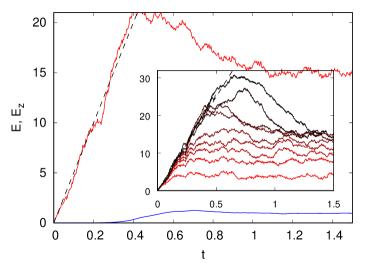
Figure 1: Time evolution of the total kinetic energy $E$ (red line) and of the vertical kinetic energy $E_{z}$ (blue line) for the forced run $6$ at $S=0.25$. The black dashed line represents the growth rate due to the energy input, $\varepsilon_{I}t$. Inset: Time evolution of the total kinetic energy $E$ for all the runs. Thickness $S$ (and Run number) increases from bottom (red) to top (black) lines. The black dashed line represents $\varepsilon_{I}t$.

From Fig. 1 we can clearly distinguish two phases in the turbulent flow: a two-dimensional regime at initial times and a three-dimensional regime at late times. This picture is observed (with quantitative differences) for all the simulations at different thickness as shown in the inset of Fig. 1. The fact that kinetic energy reaches a constant value indicates that, for any thickness, the flow is unable to sustain an inverse cascade (which would keep the energy increasing). The reason why the energy split scenario (in which both a direct and an inverse energy cascades are present) is not observed in our simulations is the main result of our work and will be discussed in details below.

From Fig. 1 we observe that the asymptotic value of the energy grows with the thickness, more rapidly for lower values of $S$. This is shown more clearly in Fig. 2 together with the dependence of $E_{z}/E$ on $S$ in stationary conditions. We see that for $S\lesssim 0.3$ the asymptotic energy has a strong dependence on $S$, while for larger values of the thickness, $E$ reaches an almost constant plateau. The inset of Fig. 2 displays the dependence of the ratio $E_{z}/E$ with the thickness. In this case we observe a growth for all the values of $S$, indicating that the presence of the bottom boundary affects the vertical motion even at $S\approx 1$. We remark that the flow remains anisotropic also at large $S$ since $E_{z}/E<1/3$.

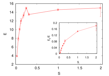
Figure 2: Asymptotic kinetic energy $E$ as a function of the thickness $S$. Inset: ratio $E_{z}/E$ as a function of $S$.

Since the flow has no mean velocity, $\langle{\bf u}\rangle=0$, it is natural to consider the vertical profiles of the rms velocities, i.e. ${\bm{u}}_{rms}(z)=\langle{\bm{u}}({\bf x})^{2}\rangle^{1/2}$. The different boundary conditions on the horizontal $(u,v)$ and vertical $w$ components, together with the $2D$ forcing, produce different profiles for the horizontal and vertical components.

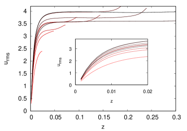
Figure 3: Vertical profile of the horizontal velocity fluctuations $u_{rms}$. The inset shows the behavior close to the boundary at $z=0$. Colors as in the inset of Fig. 1.

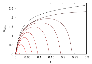
Figure 4: Vertical profile of the vertical velocity fluctuations $w_{rms}$. Colors as in the inset of Fig. 1.

Fig. 3 shows the vertical profiles of one component of the horizontal velocity $u_{rms}$ in stationary conditions. We observe, close to $z=0$, a boundary layer region, strongly affected by the presence of the bottom wall, where velocity fluctuations increase rapidly with $z$. For larger values of $z$ (and not too small $S$) horizontal velocity fluctuations saturates to an approximately constant value which increases with $S$. In these cases, we observe that close to the upper boundary $z=L_{z}$, the horizontal velocity fluctuations increase. This is a consequence of the free-slip boundary conditions and has been already observed in free-surface channel flow [18, 25]. A possible explanation of this effect is obtained from a Taylor expansion of the velocity field close to the surface $z=L_{z}$. Introducing, for simplicity of notation, the shifted variable $Z=L_{z}-z$ (such that the free surface is at $Z=0$), boundary conditions imply for one horizontal component of the velocity $u({\bf x})=u_{0}(x,y)+u_{2}(x,y)Z^{2}+O(Z^{4})$. Therefore, the variance of the velocity close to the surface has the expression

$$\langle u^{2}\rangle=\langle u_{0}^{2}\rangle+2\langle u_{0}u_{2}\rangle Z^{2}+O(Z^{4}).$$ (2)

Assuming that the energy dissipation rate averaged over horizontal planes is independent on $z$ (which is verified in our simulation for values of $z$ not too close to the bottom plane), we expect that $\langle\varepsilon\rangle=-a\nu\langle u\nabla^{2}u\rangle>0$, where the positive constant $a$ depends on the details of the flow ($a=3$ for isotropic turbulence). By Taylor expansion we can write

$$u\nabla^{2}u\simeq(u_{0}+u_{2}Z^{2})(\partial_{x}^{2}+\partial_{y}^{2}+\partial_{Z}^{2})(u_{0}+u_{2}Z^{2})\,.$$ (3)

Using integration by part in the periodic directions $x$ and $y$ we obtain

$$\langle u\nabla^{2}u\rangle=-\langle(\partial_{x}u)^{2}\rangle-\langle(\partial_{y}u)^{2}\rangle+2\langle u_{0}u_{2}\rangle+O(Z^{2})\simeq-\varepsilon/\nu<0.$$ (4)

This expression suggests that, in the absence of cancellations of leading terms, $\langle u_{0}u_{2}\rangle\propto-\varepsilon/\nu<0$ and therefore, from (2), that $\langle u^{2}\rangle$ deceases moving away from the free surface as observed in Fig. 3. A parabolic fit of the velocity variance close to $z=L_{z}$ is quantitatively consistent with the above predictions. Close to the bottom boundary with no-slip BC we observe that the extension of the boundary layer region is weakly dependent on $S$, as it is shown in the inset of Fig. 3.

Vertical profiles of the vertical velocity fluctuations are shown in Fig. 4. At variance with the horizontal components, here the velocity (and therefore its fluctuations) vanishes also at the upper free surface. The maximum value of fluctuations is observed approximately in the middle of the domain, even if, due to the different boundary conditions, the profiles are not symmetric with respect the central plane $z=L_{z}/2$. The ratio of the lines plotted in Fig. 4 and in Fig. 3 gives the profile of the anisotropy of the velocity field. Even for the largest values of $S$, we have that in the central part of the domain $w_{rms}/u_{rms}\simeq 0.5$.

IV Small-scale statistics and transient inverse cascade

As discussed in the previous Section, the 2D2C forcing produces initially a two-dimensional flow. This flow is non-stationary, as shown in Figs. 1, and eventually develops instabilities which result in a three-dimensional motion. In order to better understand and characterize this transition, we study the small scale statistics of the turbulent flow at different times and horizontal planes. We consider here the run at $S=2$ for which the results are more clear, but a similar scenario is observed for the other thickness also.

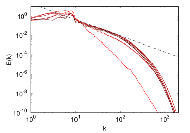
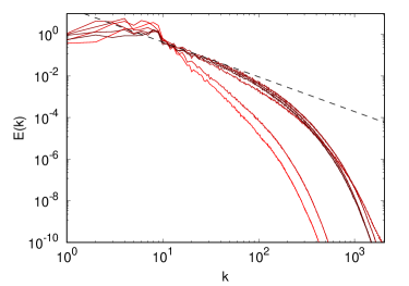
Figure 5: 2D energy spectra for the simulation at $S=2$ computed at $z=L_{z}/4$ (left) and $z\simeq L_{z}$ (right) at different times, from $t=0.2$ (light red) to time $t=1.2$ (black) with steps $\Delta t=0.2$. The dashed line represents the Kolmogorov spectrum $k^{-5/3}$.

Figure 5 shows the horizontal spectra (computed on the ($x,y$) plane) of the full velocity field in two different depth $z$ and at different times. Both at $z=L_{z}/4$ and at $z\simeq L_{z}$ (i.e. close to the lower and upper boundary respectively) the flow initially (at $t=0.2$) develops fluctuations at small scales (i.e. at $k>k_{f}=8$) with a steep spectrum compatible with a 2D direct cascade of enstrophy. During this first stage, in which the energy increases approximately with the energy injection (see Fig. 1), the flow transfers some energy at large scale as prescribed by a two-dimensional phenomenology. At $t=0.4$ the flow close to the bottom has already developed a Kolmogorov scaling $k^{-5/3}$, compatible with a 3D direct cascade, while the spectrum of the flow close to the surface is still steep (second line from bottom in both plots). At later times $t\geq 0.6$, spectra display a Kolmogorov scaling in both planes.

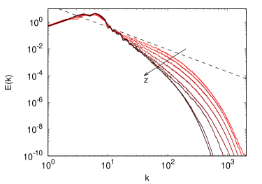
Figure 6: 2D energy spectra from the simulation at $S=2$ at time $t=0.4$ computed at different planes from $z=L_{z}/8$ (clear red) to $L_{z}\simeq L_{z}$ (black). The dashed line represents the Kolmogorov spectrum $k^{-5/3}$.

The interpretation of these results is that two-dimensional turbulence, which is initially produced by the 2D2C forcing, is transient and the flow develops a three-dimensional direct cascade starting from the layers closer to the bottom boundary. In this sense, the transition from 2D to 3D flow is not uniform in space, but proceeds from the bottom layer towards the top layer. This is clearly shown in Fig. 6, where we plot the energy spectra computed on different horizontal planes in the domain at the intermediate time $t=0.4$. It is clear that, while the upper layers (at $z\simeq L_{z}$) have a steep spectra compatible with a direct 2D cascade, the lower layers close to the bottom have already developed a 3D cascade with a Kolmogorov spectrum.

The transition from 2D to 3D dynamics at different layers is confirmed by the analysis of structure functions (SF) in physical space, in particular by the third-order SF which contains information about the flux of energy [26].

From the longitudinal velocity increments $\delta u_{L}(\ell,{\bm{x}},t)\equiv({\bm{u}}({\bm{x}}+{\bm{\ell}},t)-{\bm{u}}({\bm{x}},t))\cdot{\bm{\ell}}/\ell$ where ${\bm{\ell}}$ is a vector on the $(x,y)$ plane, we define the SF of order $p$ as

$$S_{p}(\ell;z)=\langle\delta u_{L}^{p}(\ell,{\bm{x}},t)\rangle$$ (5)

where, as in Section I, the average is over the plane $(x,y)$ and time. We remark that three-dimensional turbulence is characterized by a negative third-order SF corresponding to a direct cascade of turbulent fluctuations to small scales. In particular, in 3D homogeneous-isotropic turbulence one has $S_{3}(\ell)=-(4/5)\varepsilon\ell$ [27]. In two dimensions one has, on the contrary, an inverse cascade of turbulent fluctuations at scales larger than $L_{f}$ with a positive third-order SF given, in homogeneous-isotropic conditions, by $S_{3}(\ell)=(3/2)\varepsilon\ell$ [26].

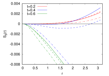
Figure 7: Horizontal longitudinal third-order velocity structure functions $S_{3}({\ell;z})$ computed at three times of the simulation, $t=0.2$ (red lines), $t=0.4$ (blues lines) and $t=0.6$ (green lines). Continuous lines correspond to $z=3/4L_{z}$, dashed line to $z=1/2L_{z}$ and dashed-dotted line to $z=1/4L_{z}$. Simulation at $S=2$.

In Fig. 7 we plot the horizontal third-order longitudinal velocity SF at three different times and at three different depth corresponding to $z/L_{z}=1/4,1/2,3/4$. At short time, $t=0.2$ the SF is positive, corresponding to an inverse energy cascade, at all the three depths considered, consistent with the spectrum shown in Fig. 4. At the intermediate time $t=0.4$ (which still correspond to the growing phase of the total energy, see inset of Fig. 1), the SF in the upper layer (continuous line) is still positive, while it becomes negative in the lower layer close to the bottom boundary (dotted-dashed line). At the intemediate layer the SF change sign with the scale and at large scales is still positive. This confirms the picture in Fourier space observed in Fig. 6. At time $t=0.6$, which corresponds to the peak of the kinetic energy in Fig. 1, the SFs become negative for all the depth considered, indicating a complete transition to 3D turbulence in the whole domain. This is at variance to what observed in simulations in fully periodic domains where, for intermediate values of $S$, it is observed an inverse cascade at large scales together with a direct cascade at small scales, both in stationary conditions [2]. Remarkably, laboratory experiments in a conducting fluid show a similar phenomenology with the transion from positive to negative third-order SF [28].

The physical interpretation of these results, which are qualitatively confirmed also for the other simulations at smaller $S$, is that the 2D2C forcing initially produces a quasi two-dimensional flow, which is turbulent (positive $S_{3}(\ell)$) in the whole domain. As the energy increases, the friction on the bottom boundary induces vertical motions which make the flow three-dimensional (negative $S_{3}(\ell)$) starting from the lower layers. Eventually, at longer times, the whole flow becomes three dimensional, turbulent fluctuations are dissipated by viscosity and the kinetic energy decreases to reach a stationary state.

V Decaying turbulence

In order to better understand the effects of the bottom layer on the turbulent flow, we performed additional simulations in decaying conditions, i.e. by integrating (1) without the forcing term ${\bm{f}}$. The initial conditions for the decaying simulations are taken from the forced runs in stationary conditions, i.e. from the last time of the inset of Fig. 1.

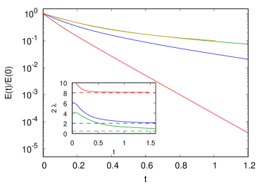
Figure 8: Decaying of total kinetic energy in unforced simulations at different thickness $S=0.03125$ (red lower line), $S=0.0625$ (blue intermediate line), $S=0.125$ and $S=0.3125$ (green and orange upper lines). Inset: local exponential slope of $\log(E(t)/E(0))$ for simulations at $S=0.03125$ (red upper line), $S=0.0625$ (blue intermediate line), $S=0.125$ (green lower line). Dashed lines represent the viscous decay rate $\lambda=\pi^{2}\nu/(4L_{z}^{2})$.

The evolution of the energy (normalized with the initial energy $E(0)$) is shown in Fig. 8 (where the initial time $t=0$ is now the time at which the forcing is switched off). From a qualitative point of view, it is evident that the decay is faster for thinner layers, indicating the importance of the bottom boundary for the dissipation of energy. Nonetheless, we see that energy dissipation rate becomes almost independent in the case of thick layers (the lines for $S=0.125$ and $S=0.3125$ are practically identical).

The lin-log plot of Fig. 8 suggests that, while in the thinnest case $S=0.03125$ the long-time decay is with good approximation exponential, this is not the case for the simulations at larger values of $S$. This is quantitatively confirmed by the inset of Fig. 8 where we plot the local rate of exponential decay for three cases. The rate $2\lambda$ is obtained by plotting the local slope of $\log(E(t)/E(0))$ vs time, while the dashed lines represent the theoretical viscous decaying rate of a 2D flow with friction, given by $\lambda=\nu\pi^{2}/(4L_{z}^{2})$ [13]. It is clear that, while the flow at $S=0.03125$, after a short transient, reaches the exponential decay with the predicted viscous rate, the other cases with larger $S$ display a more complex decay law which cannot be simply described by an exponential law and a corresponding friction coefficient $\lambda$. A complex decaying law in quasi 2D experiments has been recently reported and interpreted as different stages of exponential decay with different decaying constant [29]. The results shown in the inset of Fig. 8 indicate that in our case it is difficult to recognize a, even transient, exponential regime and that the interplay of 2D and 3D motion produces a complex decaying phenomenology.

VI Conclusions

We studied the dynamics and statistics of turbulence in a thin layer with no-slip BC on the bottom surface, forced by a 2D2C forcing. For the range of thickness explored, we find that the flow is unable to sustain an inverse energy cascade: after a initial transient, the flow develops a three-dimensional direct cascade which starts from the bottom and eventually propagates in the whole domain. The analysis of the energy spectrum and of the third-order structure function shows that at intermediate times, a 2D like and a 3D like phenomenologies can coexist at different depth in the flow. This is in contrast to what observed in homogeneous simulations in the absence of boundaries where the the flow can sustain simultaneously an inverse cascade of energy to large scales and a direct cascade to small scales [2]. Moreover, our results are also at odds with several laboratory experiments where an inverse cascade is observed [30, 17, 31, 14, 15], but mostly in the presence of two layers of fluids (miscible or not). The differences in these cases are probably due to the fact that the dynamics in the upper layer (where the flow is studied), is partially decoupled from the lower layer which is affected by the no-slip boundary conditions.

Finally, we studied the decaying behavior of the thin turbulent layer. Also in this case we find differences with respect to laboratory experiments where the decay of kinetic energy is exponential and therefore it is parameterized by a single friction coefficient [13]. We observe a clear exponential decay only for the simulation with the thinnest layer, while in the other cases a more complex decay law is observed. The different behavior in this case can be not only ascribed to the presence of stratification, but also to the different initial flow conditions between experiments and simulations.

In this work we have changed only one parameter of the flow (the thickness $S$), while there are other variables which can produce a different phenomenology, mainly the viscosity (i.e. the Reynolds number) and the forcing statistics [32]. Further work is therefore needed to uncover the reach phenomenology of turbulent thin layers.

References

- Smith et al. [1996] L. M. Smith, J. R. Chasnov, and F. Waleffe, Crossover from two-to three-dimensional turbulence, Phys. Rev. Lett. 77, 2467 (1996).
- Celani et al. [2010] A. Celani, S. Musacchio, and D. Vincenzi, Turbulence in more than two and less than three dimensions, Phys. Rev. Lett. 104, 184506 (2010).
- Alexakis and Biferale [2018] A. Alexakis and L. Biferale, Cascades and transitions in turbulent flows, Phys. Reports 767, 1 (2018).
- Musacchio and Boffetta [2017] S. Musacchio and G. Boffetta, Split energy cascade in turbulent thin fluid layers, Phys. Fluids 29, 111106 (2017).
- Deusebio et al. [2014] E. Deusebio, G. Boffetta, E. Lindborg, and S. Musacchio, Dimensional transition in rotating turbulence, Phys. Rev. E 90, 023005 (2014).
- Sozza et al. [2015] A. Sozza, G. Boffetta, P. Muratore-Ginanneschi, and S. Musacchio, Dimensional transition of energy cascades in stably stratified forced thin fluid layers, Phys. Fluids 27, 035112 (2015).
- Clark et al. [2021] D. Clark, A. Armua, C. Freeman, D. J. Brener, and A. Berera, Chaotic measure of the transition between two-and three-dimensional turbulence, Phys. Rev. Fluids 6, 054612 (2021).
- Xia et al. [2009] H. Xia, M. Shats, and G. Falkovich, Spectrally condensed turbulence in thin layers, Phys. Fluids 21, 125101 (2009).
- Laurie et al. [2014] J. Laurie, G. Boffetta, G. Falkovich, I. Kolokolov, and V. Lebedev, Universal profile of the vortex condensate in two-dimensional turbulence, Phys. Rev. Lett. 113, 254503 (2014).
- Musacchio and Boffetta [2019] S. Musacchio and G. Boffetta, Condensate in quasi-two-dimensional turbulence, Phys. Rev. Fluids 4, 022602 (2019).
- van Kan and Alexakis [2019] A. van Kan and A. Alexakis, Condensates in thin-layer turbulence, J. Fluid Mech. 864, 490 (2019).
- Fang and Ouellette [2021] L. Fang and N. T. Ouellette, Spectral condensation in laboratory two-dimensional turbulence, Phys. Rev. Fluids 6, 104605 (2021).
- Shats et al. [2010] M. Shats, D. Byrne, and H. Xia, Turbulence decay rate as a measure of flow dimensionality, Phys. Rev. Lett. 105, 264501 (2010).
- Byrne et al. [2011] D. Byrne, H. Xia, and M. Shats, Robust inverse energy cascade and turbulence structure in three-dimensional layers of fluid, Phys. Fluids 23, 095109 (2011).
- Xia et al. [2011] H. Xia, D. Byrne, G. Falkovich, and M. Shats, Upscale energy transfer in thick turbulent fluid layers, Nature Phys. 7, 321 (2011).
- Van Heijst and Clercx [2009] G. F. Van Heijst and H. J. Clercx, Studies on quasi-2d turbulence—the effect of boundaries, Fluid Dyn. Res. 41, 064002 (2009).
- Chen et al. [2006] S. Chen, R. E. Ecke, G. L. Eyink, M. Rivera, M. Wan, and Z. Xiao, Physical mechanism of the two-dimensional inverse energy cascade, Phys. Rev. Lett. 96, 084502 (2006).
- Nagaosa [1999] R. Nagaosa, Direct numerical simulation of vortex structures and turbulent scalar transfer across a free surface in a fully developed turbulence, Phys. Fluids 11, 1581 (1999).
- Olivieri et al. [2020] S. Olivieri, L. Brandt, M. E. Rosti, and A. Mazzino, Dispersed fibers change the classical energy budget of turbulence via nonlocal transfer, Phys. Rev. Lett. 125, 114501 (2020).
- Rosti and Takagi [2021] M. E. Rosti and S. Takagi, Shear-thinning and shear-thickening emulsions in shear flows, Phys. Fluids 33, 083319 (2021).
- Mazzino and Rosti [2021] A. Mazzino and M. E. Rosti, Unraveling the secrets of turbulence in a fluid puff, Phys. Rev. Lett. 127, 094501 (2021).
- Brizzolara et al. [2021] S. Brizzolara, M. E. Rosti, S. Olivieri, L. Brandt, M. Holzner, and A. Mazzino, Fiber tracking velocimetry for two-point statistics of turbulence, Phys. Rev. X 11, 031060 (2021).
- Mazzino and Rosti [2022] A. Mazzino and M. E. Rosti, Puff turbulence in the limit of strong buoyancy, Philos. Trans. Roy. Soc. A 380, 20210093 (2022).
- Hori et al. [2022] N. Hori, M. E. Rosti, and S. Takagi, An eulerian-based immersed boundary method for particle suspensions with implicit lubrication model, Comput. Fluids 236, 105278 (2022).
- Lovecchio et al. [2013] S. Lovecchio, C. Marchioli, and A. Soldati, Time persistence of floating-particle clusters in free-surface turbulence, Phys. Rev. E 88, 033003 (2013).
- Boffetta and Ecke [2012] G. Boffetta and R. E. Ecke, Two-dimensional turbulence, Annu. Rev. Fluid Mech. 44, 427 (2012).
- Frisch [1995] U. Frisch, Turbulence: the legacy of AN Kolmogorov (Cambridge University Press, 1995).
- Gledzer et al. [2011] A. Gledzer, E. Gledzer, A. Khapaev, and O. Chkhetiani, Structure functions of quasi-two-dimensional turbulence in a laboratory experiment, J. Exp. Theor. Phys. 113, 516 (2011).
- Fang and Ouellette [2017] L. Fang and N. T. Ouellette, Multiple stages of decay in two-dimensional turbulence, Phys. Fluids 29, 111105 (2017).
- Paret and Tabeling [1997] J. Paret and P. Tabeling, Experimental observation of the two-dimensional inverse energy cascade, Phys. Rev. Lett. 79, 4162 (1997).
- von Kameke et al. [2011] A. von Kameke, F. Huhn, G. Fernández-García, A. P. Muñuzuri, and V. Pérez-Muñuzuri, Double cascade turbulence and richardson dispersion in a horizontal fluid flow induced by faraday waves, Phys. Rev. Lett. 107, 074502 (2011).
- Poujol et al. [2020] B. Poujol, A. van Kan, and A. Alexakis, Role of the forcing dimensionality in thin-layer turbulent energy cascades, Phys. Rev. Fluids 5, 064610 (2020).