Semilocal Meta-GGA Exchange-Correlation Approximation From Adiabatic Connection Formalism: Extent and Limitations

Abstract

The incorporation of a strong interaction regime within the approximate, semilocal exchange-correlation functionals still remains a very challenging task for density functional theory. One of the promising attempts in this direction is the recently proposed adiabatic connection semilocal correlation (ACSC) approach [Phys. Rev. B 2019, 99, 085117] allowing to construct the correlation energy functionals by interpolation of the high and low-density limits for the given semi-local approximation. The current study extends the ACSC method to the meta-GGA level of theory, providing some new insights. As an example, we construct the correlation energy functional base on the high and low-density limits of the Tao-Perdew-Starverov-Scuseria (TPSS) functional. Arose in this way TPSS-ACSC functional is one electron self-interaction free, accurate for the strictly correlated, and quasi-two-dimensional regimes. Based on simple examples, we show the advantages and disadvantages of ACSC semi-local functionals and provide some new guidelines for future developments in this context.

I Introduction

The electronic structure calculations of quantum chemistry, solid-state physics, and material sciences become enormously simple since the advent of the Kohn-Sham (KS) Kohn and Sham (1965); Hohenberg and Kohn (1964) density functional theory (DFT) Burke (2012). In DFT, the development of efficient yet accurate exchange-correlation (XC) functional, which contains all the many-body quantum effects beyond the Hartree method, is one of the main research topics since the last couple of decades and continues to be the same in recent times. The accuracy of the ground-state properties of electronic systems depends on the XC functional approximation (density functional approximation - DFA). The non-empirical XC functionals are developed by satisfying many quantum mechanical exact constraints Levy (2010, 2016); Sun et al. (2015); Tao and Mo (2016) such as: density scaling rules of XC functionals due to coordinate transformations Levy and Perdew (1985); Levy (2016); Görling and Levy (1992); Fabiano and Constantin (2013), second (and fourth) order gradient expansion of exchange and correlation energies Svendsen and von Barth (1996); Antoniewicz and Kleinman (1985); Hu and Langreth (1986); Ma and Brueckner (1968); Argaman et al. (2022); Daas et al. (2022a, b), low density, and high density limit of the correlation energy functionalGörling and Levy (1994, 1993, 1995), asymptotic behavior of the XC energy density or potential Della Sala and Görling (2002); Engel et al. (1992); Horowitz et al. (2009); Constantin and Pitarke (2011); Constantin et al. (2016a); Niquet et al. (2003); Almbladh and von Barth (1985); Umrigar and Gonze (1994), quasi-2D behavior of the XC energy Pollack and Perdew (2000); Kaplan et al. (2018); Constantin (2016, 2008), and exact properties of the XC hole  Tao and Mo (2016); Tao et al. (2008); Přecechtělová et al. (2014, 2015).

Different rungs of Jacob’s ladder Perdew and Schmidt (2001) classification of non-empirical XC approximations are developed based on the use of various ingredients, from the simple spin densities and their gradients, until the occupied and unoccupied KS orbitals and energies Grimme (2006); Mehta et al. (2018); Bartlett et al. (2005a); Grabowski et al. (2014); Śmiga et al. (2020); Siecińska et al. (2022); Seidl et al. (2000a). The first rung of the ladder is the local density approximations (LDA)Kohn and Sham (1965). Next rungs are represented by semilocal functionals, such as generalized gradient approximations (GGA) Perdew et al. (1996a); Scuseria and Staroverov (2005) and meta-GGA  Tao et al. (2003); Sun et al. (2015); Tao and Mo (2016); Jana et al. (2019a); Patra et al. (2019); Jana et al. (2021a); Patra et al. (2020); Jana et al. (2021b). Higher rungs are known as 3.5 rung XC functionals Janesko and Aguero (2012); Janesko (2013, 2010, 2012); Janesko et al. (2018); Constantin et al. (2016b, 2017a), hybrids and hyper-GGAs Perdew et al. (2008, 2005); Odashima and Capelle (2009); Arbuznikov and Kaupp (2011); Jaramillo et al. (2003); Kümmel and Kronik (2008); Becke (2005); Becke and Johnson (2007); Becke (2003, 2013); Patra et al. (2018); Jana et al. (2018a); Jana and Samal (2019); Jana et al. (2018b, 2020a, 2019b, 2022), double hybrids Grimme and Neese (2007); Su and Xu (2014); Hui and Chai (2016); Sharkas et al. (2011); Souvi et al. (2014); Toulouse et al. (2011), and adiabatic connection (AC) random-phase approximation (RPA) like methods and DFT version of the coupled-cluster theory Toulouse et al. (2009); Ruzsinszky et al. (2016, 2010); Bates et al. (2017); Hu and Langreth (1986); Terentjev et al. (2018); Constantin (2016); Corradini et al. (1998); Erhard et al. (2016); Patrick and Thygesen (2015); Bartlett et al. (2005b, c); Grabowski et al. (2013, 2014).

Specifically, we recall that the AC formalism Langreth and Perdew (1975); Gunnarsson and Lundqvist (1976); Savin et al. (2003); Cohen et al. (2007); Ernzerhof (1996); Burke et al. (1997); Colonna and Savin (1999), used in various sophisticated XC functionals  Savin et al. (2003); Ernzerhof (1996); Burke et al. (1997); Toulouse et al. (2009); Patrick and Thygesen (2015); Cohen et al. (2007); Colonna and Savin (1999); Adamo and Barone (1998); Perdew et al. (2001); Liu and Burke (2009); Magyar et al. (2003); Sun (2009); Seidl and Gori-Giorgi (2010); Vuckovic et al. (2016a); Fabiano et al. (2019); Vuckovic et al. (2018); Kooi and Gori-Giorgi (2018); Seidl et al. (2018); Constantin (2019), is based on the coupling constant (or interaction strength) integral formula Langreth and Perdew (1975); Savin et al. (2003); Cohen et al. (2007); Ernzerhof (1996); Burke et al. (1997)

$$E_{xc}[n]=\int_{0}^{1}~{}d\alpha~{}W_{\alpha}[n]~{},$$

$$W_{\alpha}[n]=\langle\Psi_{\alpha}[n]|\hat{V}_{ee}|\Psi_{\alpha}[n]\rangle-U[n],$$ (1)

where $\hat{V}_{ee}$ is the Coulomb operator, $U[n]$ is the Hartree energy, $\Psi_{\alpha}[n]$ is the anti-symmetric wave function that yields the density $n(\mathbf{r})$ and minimizes the expectation value $<\hat{T}+\alpha\hat{V}_{ee}>$, with $\hat{T}$ being the kinetic energy operator, and $\alpha$ the coupling constant. Eq. (1) can be seen as the exact definition of the XC functional, and it connects a non-interacting single particle system ($\alpha=0$) to a fully interacting one ($\alpha=1$). Note that the $\alpha\to 0$ limit is known as the weak-interaction limit ( or high-density or $r_{s}\to 0$ limit, where $r_{s}$ is the local Seitz radius), where the perturbative approach is valid. Thus, the well-known second-order Görling-Levy perturbation theory (GL2) Görling and Levy (1994, 1993, 1995); Görling (1998) can be applied in the weak-interaction limit, and $W_{\alpha}[n]$ can be expanded as Seidl et al. (2000a)

$$W{{}_{\alpha\to 0}}[n]=W_{0}[n]+W_{0}^{\prime}[n]\alpha~{}+\dots$$ (2)

where $W_{0}=E_{x}$ and $W_{0}^{\prime}[n]=2E_{c}^{GL2}[n]$. On the other hand, the strong-interaction limit ( or low-density or $r_{s}\to\infty$ limit) of $W_{\alpha}[n]$ is given as Seidl et al. (2000b, a); Gori-Giorgi et al. (2009a); Liu and Burke (2009)

$${{\color[rgb]{0,0,0}W{{}_{\alpha\to\infty}}[n]=W_{\infty}[n]+W_{\infty}^{\prime}[n]\alpha^{-1/2}+O(\alpha^{-p})\dots,~{}~{}~{}p\geq 3/4}}$$ (3)

where $W_{\infty}[n]$ and $W_{\infty}^{\prime}[n]$ have a highly non-local density dependence, captured by the strictly-correlated electrons (SCE) limit Seidl et al. (2007); Gori-Giorgi et al. (2009b); Malet et al. (2013), and their exact evaluation in general cases is a non-trivial problem.

In particular, one of the successful attempts at practical usability of the AC DFAs came through the interaction strength interpolation (ISI) method by Seidl and coworkers Seidl et al. (2000a, b); Perdew et al. (2001); Seidl and Gori-Giorgi (2010); Gori-Giorgi et al. (2009a); Gori-Giorgi and Seidl (2010); Fabiano et al. (2016); Seidl et al. (1999a, 2018, 2016) where the DFA formula is built by interpolating between the weak- and strong interaction regimes. The $\alpha\to\infty$ limit is approximated by semilocal gradient expansions (GEA) derived within the point-charge-plus-continuum (PC) model Seidl et al. (2000a, b); Perdew et al. (2001); Seidl and Gori-Giorgi (2010). Based on this form, the ISI has been tested for various applications Fabiano et al. (2016); Giarrusso et al. (2018); Fabiano et al. (2019). Also, several modifications of the ISI have been suggested Mirtschink et al. (2012); Gori-Giorgi et al. (2009a); Liu and Burke (2009); Seidl et al. (1999b); Daas et al. (2021) as well as the PC model itself such as the hPCŚmiga et al. (2022) or modified PC (mPC) Constantin (2019) which was found to be more robust for the quasi-two dimensional (quasi-2D) density regime.

Recently, based on the ISI formula, the adiabatic connection semilocal correlation (ACSC) method was introducedConstantin (2019), showing the alternative path of construction of semilocal correlation energy functionals. The ACSC formula interpolates the high and low-density limit for the given semi-local DFA directly, contrary to the standard path where the interpolation is done at the local LDA level and then corrected by gradient or meta-GGA correctionsPerdew et al. (1996a); Tao et al. (2003). We recall that in Refs. Constantin, 2019, the ACSC functional was built using Perdew-Burke-Ernzerhof (PBE)Perdew et al. (1996a) high-density formula and mPC model showing similar or improved accuracy over its PBE precursor proving in the same time the evidence for the robustness of ACSC construction.

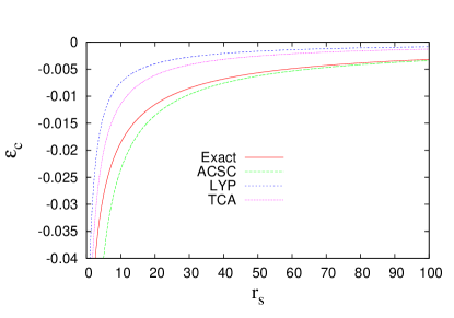
Figure 1: Correlation energy per particle $\epsilon_{c}$ versus the bulk parameter $r_{s}=(\frac{3}{4\pi n})^{1/3}$, for the uniform electron gas. See text for details of the methods and exact reference curve.

Motivated by the progress in this direction, this paper extends the ACSC method at the meta-GGA level and provides new insights in this context.

In the following, we briefly recall some aspects of ACSC functional construction and investigate a few available approximations for the high- and low-density regimes. Based on that, we propose an extension of the ACSC method to the meta-GGA level using the high and low-density limits of the Tao-Perdew-Staroverov-Scuseria (TPSS) Tao et al. (2003) DFA. Following that, we apply ACSC correlation energy functionals to some model systems (Hooke’s atom and H₂ molecule) and real calculations (the atomization energies of several small molecules) to show some advantages and current limitations of ACSC functional construction. Lastly, we conclude by discussing the possible advances of the present construction.

II Theory

II.1 Background of the Adiabatic Connection Semilocal Correlation (ACSC)

Following Ref. Constantin (2019), the ACSC correlation energy per particle is given as (Eq.(15) of ref. Constantin (2019)),

$$n\epsilon_{c}^{ACSC}(\mathbf{r})=\int_{0}^{1}d\alpha\;w_{c,\alpha}(\mathbf{r})$$ (4)

$$w_{c,\alpha}(\mathbf{r})=w_{\infty}(\mathbf{r})-w_{0}(\mathbf{r})+\frac{\mathcal{X}(\mathbf{r})}{\sqrt{1+\mathcal{Y}(\mathbf{r})\alpha}+\mathcal{Z}(\mathbf{r})}$$ (5)

$$n\epsilon_{c}^{ACSC}(\mathbf{r})=w_{\infty}(\mathbf{r})-w_{0}(\mathbf{r})$$

$$+\frac{2\mathcal{X}(\mathbf{r})}{\mathcal{Y}(\mathbf{r})}[\sqrt{1+\mathcal{Y}(\mathbf{r})}-1-\mathcal{Z}(\mathbf{r})\ln(\frac{\sqrt{1+\mathcal{Y}(\mathbf{r})}+\mathcal{Z}(\mathbf{r})}{1+\mathcal{Z}(\mathbf{r})})]~{}.$$

(6)

The above expression represents a general form for the correlation energy density derived from the ISI formula Seidl et al. (2000a, b); Perdew et al. (2001); Seidl and Gori-Giorgi (2010); Gori-Giorgi et al. (2009a); Gori-Giorgi and Seidl (2010); Fabiano et al. (2016); Seidl et al. (1999a, 2018, 2016) with

$$\mathcal{X}(\mathbf{r})=-2w^{\prime}_{0}(\mathbf{r})(w^{\prime}_{\infty}(\mathbf{r}))^{2}/(w_{0}(\mathbf{r})-w_{\infty}(\mathbf{r}))^{2},$$

$$\mathcal{Y}(\mathbf{r})=4(w^{\prime}_{0}(\mathbf{r}))^{2}(w^{\prime}_{\infty}(\mathbf{r}))^{2}/(w_{0}(\mathbf{r})-w_{\infty}(\mathbf{r}))^{4},$$

$$\mathcal{Z}(\mathbf{r})=-1-2w^{\prime}_{0}(\mathbf{r})(w^{\prime}_{\infty}(\mathbf{r}))^{2}/(w_{0}(\mathbf{r})-w_{\infty}(\mathbf{r}))^{3}.$$

(7)

and where $w_{0}$, $w^{\prime}_{0}$, and $w_{\infty}$, $w^{\prime}_{\infty}$ denote the approximation for energy densities for high- ( or weak-interaction) and low-density ( or strong-interaction) limits, respectively.

Considering the accuracy of Eq. (4), it depends on three main aspects:

• the interpolation formula is used to define the $w_{c,\alpha}(\mathbf{r})$ integrand in Eq. (4). In Refs. Constantin, 2019 (and here Eq. (5)), the ISI interpolation formula was utilized to define ACSC. We note, however, that for this choice the $W_{\alpha}[n]$ contains a spurious term proportional to $\alpha^{-1}$ in its strong-interaction limit ($\alpha\to\infty$) Seidl et al. (2000b) which has been corrected in refs. Liu and Burke (2009); Gori-Giorgi et al. (2009b). To be consistent with our previous work, we stuck with the ISI formula. Nonetheless, other possibilities also existMirtschink et al. (2012); Gori-Giorgi et al. (2009a); Liu and Burke (2009); Seidl et al. (1999b).

• the approximation for $\alpha\to\infty$ limit. Several possibilities exist, e.g., (exact treatment by employing SCE formulas (numerically expensive but feasible) or much less time consuming variants such as mPCConstantin (2019), hPCŚmiga et al. (2022) or the ones derived from semi-local DFA via the procedure described in Refs. Seidl et al., 2000b. Note that by choosing different $\alpha\to\infty$ limits, one can incorporate in ACSC formula different physics, e.g., good performance for the quasi-2D regime.

• the approximation for $\alpha\to 0$ limit. In principle, this limit can be taken into account exactly by considering the exact exchange (EXX) and GL2 limitGörling and Levy (1993); Kooi and Gori-Giorgi (2018); Vuckovic et al. (2016b). However, evaluation of the GL2 correlation energy density on the numerical grid would likely be computationally expensive. Hence, in Refs. Constantin, 2019, the non-local contributions have been substituted by semi-local high-density counterparts obtained from PBE functionalPerdew et al. (1996a).

This work extends the ACSC DFA by considering all input quantities at the semi-local (SL) meta-GGA level. For instance the $w_{0}(\mathbf{r})$ and $w_{0}^{\prime}(\mathbf{r})$ approximations are constructed as

$$w_{0}(\mathbf{r})=n(\mathbf{r})\epsilon_{x}^{SL}(n(\mathbf{r}),\nabla n(\mathbf{r}),\nabla^{2}n(\mathbf{r}),\tau(\mathbf{r})),$$

$$w^{\prime}_{0}(\mathbf{r})=2n(\mathbf{r})\epsilon_{c}^{SL-GL2}(n(\mathbf{r}),\nabla n(\mathbf{r}),\nabla^{2}n(\mathbf{r}),\tau(\mathbf{r}),\zeta(\mathbf{r})),$$

(8)

using SL form of the GL2 correlation energy density (SL-GL2) Constantin (2019), where $\tau(\mathbf{r})=\sum_{j}^{occ}|\nabla\phi_{j}(\mathbf{r})|^{2}/2$ is the KS non-interacting kinetic energy density, with $\phi_{j}(\mathbf{r})$ being the one-particle $j$-th occupied KS orbital. We underline that the Laplacian of the density ($\nabla^{2}n$) contains information that is is already encapsulated in $\tau$ Śmiga et al. (2017), such that many meta-GGA XC functionals do not consider $\nabla^{2}n$ as an ingredient.

There are also two prime motivations behind the extension of ACSC functionals to the meta-GGA level:

• many of SL-GL2 correlation energy functionals, such as TPSS-GL2 (and all TPSS-like GL2 functionals) have already been derived Perdew et al. (1996b, 2008); thus, they can be easily applied in the present construction. The quantitative comparison of the accuracy of these SL-GL2 models with reference second-order GL2 correlation energy data was reported in Refs. Śmiga and Constantin, 2020 in Table S12.

• the meta-GGA SL-GL2, such as TPSS-GL2 DFA, is one electron self-interaction free, giving precisely zero for the hydrogen atom, which is not the case for PBE-GL2.

In the next section, we will address the choice of $w_{\infty}(\mathbf{r})$ and $w^{\prime}_{\infty}(\mathbf{r})$.

II.2 TPSS-ACSC correlation functionals formula

To construct ACSC meta-GGA DFA, we fix the $w_{0}(\mathbf{r})$ and $w^{\prime}_{0}(\mathbf{r})$ (where the energy density $w_{\alpha}(\mathbf{r})$ is defined by $W_{\alpha}=\int~{}d\mathbf{r}~{}w_{\alpha}(\mathbf{r})$) in the form of TPSS exchange ($w_{0}(\mathbf{r})=n(\mathbf{r})\epsilon_{x}^{TPSS}$) and TPSS-GL2 Perdew et al. (2008) ($w^{\prime}_{0}(\mathbf{r})=2n(\mathbf{r})\epsilon_{c}^{TPSS-GL2}$) , respectively. In the case of $w_{\infty}(\mathbf{r})$ and $w^{\prime}_{\infty}(\mathbf{r})$, the choice is not so simple due to various variants available in the literature. As was noted before, the form of $w_{\infty}(\mathbf{r})$ and $w^{\prime}_{\infty}(\mathbf{r})$ implies the incorporation of important physics in the ACSC formula, i.e., the quasi-2D regime via mPCConstantin (2019) model or very accurate performance for weak and strong-interaction regime via hPC model developed recentlyŚmiga et al. (2022). However, both mPC and hPC are simple GGA level approximations of SCE formulas, which are not one-electron self-interaction freeŚmiga et al. (2022). Therefore, utilizing these GGA models might impact the performance of ACSC meta-GGA DFA. To overcome this limitation, one can develop the meta-GGA model for TPSS strong-interactionPerdew et al. (2004) regime as was done in appendix D in Refs. Seidl et al., 2000b. Thus, for clarity of this paper, we recall that for any approximate XC energy DFA ($E^{DFA}_{xc}=E^{DFA}_{x}+E^{DFA}_{c}$), the corresponding coupling-constant integrand $W^{DFA}_{\alpha}$ can be derived from the following formula.

$$W_{\alpha}^{DFA}[n_{\uparrow},n_{\downarrow}]= E_{x}^{DFA}[n_{\uparrow},n_{\downarrow}]$$

$$+ \frac{d}{d\alpha}\Big{(}\alpha^{2}E_{c}^{DFA}[n_{\uparrow,1/\alpha},n_{\downarrow,1/\alpha}]\Big{)}\;.$$

by considering the strictly correlated $\alpha\to\infty$ limit.

Thus, for the low-density limit of the TPSS functional, we obtain the $W_{\infty}^{TPSS}$ (Eq. (LABEL:err1)) and $W_{\infty}^{{}^{\prime}TPSS}$ (Eq. (LABEL:eer)) expressions with their corresponding energy densities $w_{\infty}(\mathbf{r})$ and $w^{\prime}_{\infty}(\mathbf{r})$, respectively. The latter quantities incorporate all physically meaningful features, i.e., canceling one-electron self-interaction and proper behavior for the quasi-2D regime (shown later), which was also the case for the mPC modelConstantin (2019). Based on the above consideration, we construct the TPSS-ACSC correlation functional using Eq. (5) with TPSS variants of $w_{0}$, $w^{\prime}_{0}$ and $w_{\infty}$, $w^{\prime}_{\infty}$ energy densities.

The final TPSS-ACSC formula diverges to $-\infty$ when $s\rightarrow 0$ ($w^{\prime}_{0}\to-\infty$), (e.g., for the case of the uniform electron gas (UEG) model) behaving in this limit as Constantin (2019)

$$\begin{split}\lim_{w^{\prime}_{0}\to-\infty}[n\epsilon^{ACSC}_{c}]=w_{\infty}-w_{0}+2w^{\prime}_{\infty}\\ -\frac{2(w^{\prime}_{\infty})^{2}}{w_{0}-w_{\infty}}\{\ln(1+\frac{w_{0}-w_{\infty}}{w^{\prime}_{\infty}})\}~{},\end{split}$$ (10)

which reveals the ACSC DFAs accuracy for UEG (see also Fig. 3 in Refs. Constantin, 2019 for PBE-ACSC functional). On the other hand for $w^{\prime}_{0}\rightarrow 0$ it gives

$$\lim_{w^{\prime}_{0}\to 0}[n\epsilon^{ACSC}_{c}]=\frac{1}{2}w^{\prime}_{0}+\frac{1}{3}\frac{1}{(w_{0}-w_{\infty})}(w^{\prime}_{0})^{2}+\mathcal{O}((w^{\prime}_{0})^{3}),$$ (11)

such that $E_{c}^{TPSS-ACSC}=0$ whenever $E_{c}^{TPSS-GL2}=0$. The TPSS-GL2 correlation energy density vanish whenever $\tau=\tau^{W}$, and $\zeta=1$, where $\tau^{W}$ is the von Weizsäcker kinetic energy density von Weizsäcker (1935); Della Sala et al. (2015). Thus, for one-electron systems, where $E_{c}^{TPSS-GL2}=0$, the TPSS-ACSC correlation energy is exact, showing that functional is one-electron self-correlation free.

At this point, the analysis of the behavior of TPSS-ACSC correlation energy is required. In Fig. (1), we show the UEG correlation energies per particle of the exact LDAPerdew and Wang (1992) (shown by the exact line in Fig. (1). We recall that for UEG, the reduced gradient $s=0$, thus $w_{0}$ reduces to LDA exchange energy density and $w^{\prime}_{0}\to-\infty$ thus for ACSC functional we utilize the ACSC limit for UEG given by Eq. (10). For comparison we also show Lee-Yang-Parr (LYP) Lee et al. (1988), and Tognetti-Cortona-Adamo (TCA) correlation Fabiano et al. (2015); Tognetti et al. (2008); Ragot and Cortona (2004) energy densities. One can note that the ACSC formula is accurate in the low-density limit ($r_{s}\geq 20$), while in the high-density limit ($r_{s}\rightarrow 0$) diverges as $\sim r_{s}^{-1/2}$, thus faster than the exact behavior ($\sim\ln(r_{s})$). Nevertheless, in the high-density limit, the exchange energy dominates over the correlation, so the proper choice of the exchange functional part should compensate for this failure of the ACSC correlation. This can be considered a drawback of ACSC construction because it might lead to some issues with a lack of compatibility between standard semi-local exchange functionals and the ACSC correlation functionals (mutual error cancellation effect). We will address this issue in the following.

III Results & Discussion

We first test the accuracy of $W_{\infty}^{TPSS}=\int~{}d\mathbf{r}~{}w^{TPSS}_{\infty}(\mathbf{r})$ and $W_{\infty}^{{}^{\prime}TPSS}=\int~{}d\mathbf{r}~{}w^{\prime TPSS}_{\infty}(\mathbf{r})$ expressions, which is reported in Table 1 for real atoms. For comparison, we also present the data obtained for the exact SCE method Seidl et al. (2007); Gori-Giorgi et al. (2009b); Daas et al. (2022c), PC, mPC, hPC as well as PBE ($W_{\infty}^{PBE}$, $W_{\infty}^{{}^{\prime}PBE}$) formulas from Refs. Seidl et al., 2000b. In the case of $W_{\infty}$, the TPSS approximation gives the best performance measured w.r.t. SCE values (even for Ar, Kr and Xr data reported recentlyDaas et al. (2022c)) being almost three times better than the one obtained for very accurate hPC model. This is partially because the former correctly removes one-electron self-interaction in $W_{\infty}^{TPSS}$, which is taken into account in all GGA $W_{\infty}$ approximations. Nonetheless, even without Hydrogen atom contribution (reported in parenthesis), the MARE of TPSS $W_{\infty}$ presents the best performance for this model (MARE=0.44%), closely followed by hPC (MARE=0.48%) that are twice better than original PC variant.

In the case of $W^{\prime}_{\infty}$, the overall performance of the TPSS model is worse than the one observed for hPC, in line with the results reported for PC. This can be since $W_{\infty}^{{}^{\prime}TPSS}$ in the slowly varying density limit does not recover correctly the gradient expansion of the PC model. The problem lies in the $H_{2}$ function (Eq. LABEL:eer), which when $t\to 0$ gives rise to the term proportional to $t^{6}$, in comparison to the PC model, which yields here term proportional $t^{2}$. One crucial difference, however, can be noted for the TPSS formula: it correctly recovers the SCE value for the H atom, which is impossible by any GGA variant.

An additional assessment of all models is provided in Table 2 and Fig. 2, where we present results obtained for the Hooke’s atom at different confinement strengths $\omega$ (see further text for computational details). Turning our attention to Table 2, we see similar trends to those presented in Table 1 for all values of $\omega$ where exact SCE data are available. Moreover, Fig. 2 shows that in the small $\omega$ range (strong-interaction limit of the Hooke’s atom), hPC and TPSS yield the best estimation of the XC energy $E_{xc}=W_{\infty}+2W^{\prime}_{\infty}$, being slightly better than those obtained from PC model, while the mPC and PBE methods fail. Actually, mPC and PBE $W_{\infty}$ and $W^{\prime}_{\infty}$ perform very similarly in all investigated cases giving rise to large errors.

Further, we perform the comparison of $W_{\infty}$ and $W^{\prime}_{\infty}$ behaviors for all studied models for an infinite barrier model (IBM) quasi-2D electron gas of fixed 2D electron density ($r_{s}^{2D}=4$) as a function of the quantum-well thickness $L$ as was also done in Refs. Constantin, 2019. The quasi-2D is very useful for the XC functional development, being the exact constraints in several modern density functional approximations Perdew et al. (2014); Sun et al. (2015).Under uniform density limit to the quasi-2D limit, density behaves as $n_{\lambda}^{z}(x,y,z)=\lambda n(x,y,\lambda z)$ and the system approaches the 2D limit when $\lambda\to\infty$. In this limit the XC energy is finite and negative i.e., $\lim_{\lambda\to\infty}E_{xc}[n_{\lambda}^{z}(x,y,z)]>-\infty$. We report this in Fig. 3. One can note that PC and hPC models change signs even for a mild quasi-2D regime. This feature is not allowable because it can lead to non-physical positive correlation energy or total failure of ISI or ACSC correlation energy expressions in quasi-2D regimes. On the other hand, the mPC, PBE, and TPSS $W_{\infty}$ and $W^{\prime}_{\infty}$ give correct behavior for a whole range of quantum-well thickness $L$.

Table 1: The values of $W_{\infty}$ and $W^{\prime}_{\infty}$ for several atoms obtained from different models and using EXX densities. We use atomic units. The results which agree best with SCE valuesSeidl et al. (2007); Gori-Giorgi et al. (2009b) are highlighted in bold (for Ar, Kr, and Xe the SCE $W_{\infty}$ values are taken from ref. Daas et al. (2022c)). The last line of each panel reports the mean absolute relative error (MARE) [(for $W_{\infty}$ (in parenthesis) and $W^{\prime}_{\infty}$ we report the results where H results are excluded]. The $W^{\prime SCE}_{\infty}$ reference data are reported with the same precision as in the Refs. Gori-Giorgi et al., 2009b.

	SCE	PC	hPC	mPC	PBE		TPSS
$W_{\infty}$
H	-0.3125	-0.3128	-0.3293	-0.4000	-0.4169		-0.3125
He	-1.500	-1.463	-1.492	-1.671	-1.6888		-1.5122
Be	-4.021	-3.943	-3.976	-4.380	-4.4203		-3.9803
Ne	-20.035	-20.018	-20.079	-21.022	-21.2983		-19.9792
Ar	-51.555	-51.5473	-51.6158	-53.2709	-53.9322		-51.3799
Kr	-166.850	-167.3561	-167.4387	-170.3279	-172.0157		-166.7765
Xe	-322.835	-324.5206	-324.6190	-328.6846	-331.3261		-323.3446
MARE[%]		0.78 (0.89)	1.18 (0.48)	8.64 (5.41)	10.36 (6.53)		0.38 (0.44)
$W^{\prime}_{\infty}$
H	0	0.0426	0.0255	0.2918	0.243		0
He	0.621	0.729	0.646	1.728	1.517		0.728
Be	2.59	2.919	2.600	6.167	5.442		2.713
Ne	22	24.425	23.045	38.644	35.307		23.835
MARE[%]		13.71	3.05	130.67	104.94		10.10

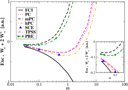
Figure 2: Comparison of the leading term of the XC energy ($E_{xc}=W_{\infty}+2W^{\prime}_{\infty}$) in the strong interaction regime of the Hooke’s atom calculated using different models with FCI dataŚmiga and Constantin (2020).

A summary of all essential features of strong-interaction models is given in Table 3. One can note that TPSS $W_{\infty}$ and $W^{\prime}_{\infty}$ reproduce reference SCE data with quite a good accuracy and some other important features, e.g., good performance in the quasi-2D regime, removes one electron self-interaction. This possibly indicates that the description of all non-local features of the SCE model can be done only by utilizing non-local ingredients such as $\tau$. This is the first important finding of the present study.

Table 2: The $W_{\infty}$ and $W^{\prime}_{\infty}$ energies (in Ha) for three values of $\omega$ for which the Hooke’s atom has analytical solutionsTaut (1993) and exact SCE reference data are availableKooi and Gori-Giorgi (2018). The last line of each panel reports the mean absolute relative error (MARE).

	SCE	PC	hPC	mPC	PBE		TPSS
$W_{\infty}$
0.0365373	-0.170	-0.156	-0.167	-0.191	-0.191		-0.170
0.1	-0.304	-0.284	-0.303	-0.344	-0.344		-0.308
0.5	-0.743	-0.702	-0.743	-0.841	-0.843		-0.754
MARE		6.78%	0.70%	12.90%	12.98%		0.96%
$W^{\prime}_{\infty}$
0.0365373	0.022	0.021	0.021	0.060	0.053		0.026
0.1	0.054	0.054	0.053	0.146	0.130		0.062
0.5	0.208	0.215	0.208	0.562	0.501		0.240
MARE		2.64%	2.13%	171.10%	139.81%		14.70%

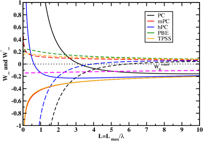
Figure 3: Comparison of $W_{\infty}$ (solid line) and $W^{\prime}_{\infty}$ (dashed line) behaviors for an IBM quasi-2D electron gas of fixed 2D electron density ($r_{s}^{2D}=4$) as a function of the quantum-well thickness $L$. Also shown is the exact exchange $W_{0}$. PC and mPC are obtained from PBE, and results are taken from ref. Constantin (2019). For PBE the $W_{\infty}$ and $W^{\prime}_{\infty}$ expression from ref. Seidl et al. (2000b). For TPSS, $W_{\infty}$ and $W^{\prime}_{\infty}$ expression are given in Eq. LABEL:err1 and Eq. LABEL:eer, respectively.

Table 3: Brief summarize of properties of $w_{\infty}(\mathbf{r})$ and $w^{\prime}_{\infty}(\mathbf{r})$ from various semi-local models.

	PC Seidl et al. (2000a, b)	mPC Constantin (2019)	hPC Śmiga et al. (2022)	PBE  Seidl et al. (2000b)	TPSSPerdew et al. (2004)
level of theory	GEA	GGA	GGA	GGA	meta-GGA
accurate for the strictly correlated regime	$\checkmark$	$\times$	$\checkmark$	$\times$	$\checkmark$
quasi-2D regime	$\times$	$\checkmark$	$\times$	$\checkmark$	$\checkmark$
self-consistent calculations	$\times$	$\checkmark$	$\checkmark$	$\checkmark$	$\checkmark$
one-electron self interaction free	$\times$	$\times$	$\times$	$\times$	$\checkmark$

Table 4: The TPSS and TPSS-ACSC correlation energies (mHa) divided by the number of electrons ($N_{e}$) for $10$ atoms (computed using Hartree-Fock analytic orbitals and densities Davidson et al. (1991); Chakravorty et al. (1993); Clementi and Corongiu (1997)) and eight molecules (computed using Hartree-Fock orbitals and densities obtained with uncontracted cc-pVTZDunning (1989) basis sets).

Atoms	$N_{e}$	TPSS	TPSS-ACSC	Ref. Davidson et al. (1991); Chakravorty et al. (1993); Clementi and Corongiu (1997)
H	1	0.0	0.0	0
He	2	-21.5	-20.2	-21
Li	3	-16.5	-15.9	-15.1
Be	4	-21.7	-20.8	-23.6
N	7	-26.5	-25.9	-26.9
Ne	10	-35.4	-35.3	-39.1
Ar	18	-39.5	-39.8	-40.1
Kr	36	-49.2	-49.9	-57.4
Zn	30	-47.0	-47.8	-56.2
Xe	54	-54.1	-55.3	-57.2
MAEatm		2.6	2.5
Molecules	$N_{e}$	TPSS	TPSS-ACSC	Ref.
H2	2	-21.1	-19.9	-19.8
LiH	4	-21.5	-20.2	-18.5
Li2	6	-21.0	-20.0	-17.9
H2O	10	-33.2	-33.1	-32.9
NH3	10	-31.9	-32.1	-30.6
HF	10	-34.3	-34.1	-33.7
CO	14	-32.4	-32.4	-34.0
N2	14	-32.7	-32.1	-30.6
MAEmol		1.7	1.2

Now, let us focus on the numerical performance of the TPSS-ACSC functional itself. In Table 4, we report the correlation energies for small atoms and molecules obtained with TPSS-ACSC and TPSS functionals energy expression. In the case of atoms, the calculations are performed using the Hartree-Fock (HF) analytic orbitals of Clementi and Roetti Clementi and Roetti (1974). For molecules, we have performed the HF calculations in ACESIIStanton et al. (2007) program using the uncontracted cc-pVTZDunning (1989) basis sets and geometries taken from refs. Grabowski et al. (2014); Śmiga et al. (2020).

We recall that using self-interaction free HF orbitals allows us to test the error specifically related to the functional construction itself, namely the functional-driven errorKim et al. (2013). As was shown in Refs. Hernandez et al., 2023, the utilization of HF densities can sometimes lead to the worsening of predictions of DFAs or improving them for the wrong reasons. This could happen when a density-driven error gives a significant contribution not canceled totally by applying the HF densities. In these cases, utilization of more accurate, correlated densities is requiredHernandez et al. (2023). However, in most semilocal DFAs, the total error is predominated by functional-driven error, meaning that HF densities are sufficiently accurate to perform such analysis.

As noted before, both considered correlation functionals are one-electron self-interaction-free, which is visible in the case of the H atom. In most cases, TPSS-ACSC performs in line with its TPSS counterpart, indicating that the correlation effects are well represented in ACSC energy expression. To visualize the correlation densities, in Fig. 4, we show a comparison between $\epsilon_{c}^{TPSS}$, $\epsilon_{c}^{TPSS-GL2}$, and $\epsilon_{c}^{TPSS-ACSC}$ for Ar atom. Whenever $s$ is small, $\epsilon_{c}^{TPSS-GL2}$ starts to depart from $\epsilon_{c}^{TPSS}$, diverging when $s=0$. However, $\epsilon_{c}^{TPSS-ACSC}$ is well-behaved everywhere.

As to the molecules, we note that TPSS-ACSC performs very well for most systems, slightly better than TPSS functional. This again confirms the robustness of correlation functional construction.

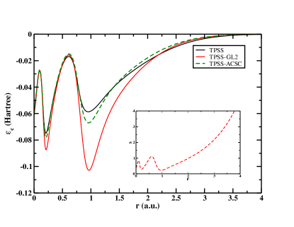
Figure 4: Correlation energy per particle $\epsilon_{c}$ versus the radial distance from the nucleus $r$, for the Ar atom. (computed using Hartree-Fock analytic orbitals and densities Davidson et al. (1991); Chakravorty et al. (1993); Clementi and Corongiu (1997)). In the inset, we show the reduced gradient $s=\frac{|\nabla n|}{2k_{F}n}$.

In Fig. 5, we report the relative error (RE) on XC energy computed for two-electron Hooke’s atoms model for various values of confinement strength $\omega$ ($\omega\in[0.03,1000]$). The errors are computed with respect to Full Configuration Interaction (FCI) results from Refs. Śmiga and Constantin, 2020. The calculations have been performed using an identical computational setup as in our previous studyŚmiga and Constantin (2020); Jana et al. (2020b, 2021a) using EXX reference orbitals. We recall that the system is strongly correlated for small values of confinement strength $\omega$, whereas we enter a weak-interaction regime for large values of $\omega$. Thus, the model provides an excellent tool for testing functional performance in these two regimes. We underline that in all following calculations, all TPSS-like correlation functionals have been combined with the TPSS exchange energy functional to obtain XC energies.

For medium and large values of $\omega$, the TPSS and TPSS-ACSC functionals perform very similarly, giving in the weak interacting region a very small relative error (RE) similar to exact GL2 and ISI XC functionals. In a strong-interaction regime, the TPSS-ACSC improves over its TPSS precursor. We note that in the latter regime, the TPSS-ACSC functional should recover, in principle, the ISI functional data due to the inclusion in both energy expressions the $W_{\infty}$ and $W^{\prime}_{\infty}$ in the form given by Eq. (LABEL:err1) and Eq. (LABEL:eer). Although qualitatively, they behave very similarly, there is a sizeable quantitative difference between these two curves. This is most probably related to the significant impact of the GL2 term, which enters both formulas. We recall that the ISI formula utilized the exact GL2 energy expression, whereas the TPSS-ACSC approximated the SL variant. Although they both diverge when $\omega$ tends to zero, the origin of that behavior is different. The exact GL2 energy diverges due to closing the HOMO-LUMO gap in this regime, whereas TPSS-GL2 is due to vanishing reduced gradient, which leads to a much faster divergence. This feature of TPSS-GL2 energy expression governs the behavior of TPSS-ACSC DFA in a small $\omega$ regime. Thus, we might conclude that the quantitative difference between ISI and TPSS-ACSC DFAs comes mainly from the inaccuracy of the SL-GL2 formula used in the later expression.

Now we turn attention to another two electron example where we may encounter a strong-interaction limit, namely, the potential energy surface for the dissociation of the H₂ molecule, in a restricted formalism Cohen et al. (2012), which is one of the main DFT challenges Cohen et al. (2012); Kirkpatrick et al. (2021); Peach et al. (2007). This is reported in Fig. 6. All energies have been obtained using EXX orbitals and densities. We want to underline that restricted HF density could give rise to substantial errors in the mid-bond region when the H₂ molecule is largely stretched. As pointed out earlier, the functional-driven error dominates most semilocal DFAs. Thus, the utilization of HF densities still gives a valid picture of the performance of semilocal DFAs for the whole range of distances of H₂.

One can note that, in general, TPSS-ACSC functional performs very similarly to TPSS, especially near equilibrium distance. More visible differences between these two DFAs can be seen for larger distances $R/R_{0}>3$. Asymptotically, the TPSS-ACSC energy goes almost to the same value as the ISI method with Eq. (LABEL:err1) and Eq. (LABEL:eer) employed to describe $W_{\infty}$ and $W^{\prime}_{\infty}$. This is an interesting finding, possibly suggesting the dominant role of strong-interaction limit (see Eq. (10)) for large separation of hydrogen atoms. We note, however, that the TPSS-GL2 total energy gives much more stable results in the asymptotic region in comparison to the exact GL2 curve, which diverges due to the closing HOMO-LUMO gap. This indicates that the proper behavior investigated here ISI and TPSS-ACSC DFAs have a different origin. In the former, the exact GL2 diverges ( $E_{GL2}\rightarrow-\infty$), leading in the asymptotic limit to $E_{xc}^{ISI}\rightarrow W_{\infty}+2W^{\prime}_{\infty}(1-\frac{1}{q}\ln(1+q))$ with $q=(E_{x}-W_{\infty})/W^{\prime}_{\infty}$ Fabiano et al. (2016); Śmiga et al. (2022). In the latter, the asymptotic limit is governed rather by the mutual error cancellation effect in TPSS-ACSC energy expression. This is because TPSS-GL2 energy expressions do not diverge for large $R/R_{0}$, meaning that at the asymptotic region Eq. 10 do not hold. One possible way to recover Eq. refszs1a within the TPSS-ACSC formula could be realized via proper incorporation of local gap modelFabiano et al. (2014); Krieger et al. (1999); Constantin et al. (2017b) within SL-GL2 formula.

Figure 5: Relative error on XC energies of harmonium atoms for various values of $\omega$ computed at @EXX orbitals for several functional using computational setup from Refs. Śmiga and Constantin, 2020. The errors have been computed with respect to FCI data obtained in the same basis setMatito et al. (2010); Śmiga and Constantin (2020). For all TPSS-like results have been obtained together with the TPSS exchange energy functional. The GL2 and ISI(TPSS) XC correlation results are obtained with the exact GL2Görling and Levy (1994) formula combined with EXX energy expression. The ISI formula utilizes the $W_{\infty}$ and $W^{\prime}_{\infty}$ given by Eq. (LABEL:err1) and Eq. (LABEL:eer). Exact ISI data are taken from Refs. Kooi and Gori-Giorgi, 2018.

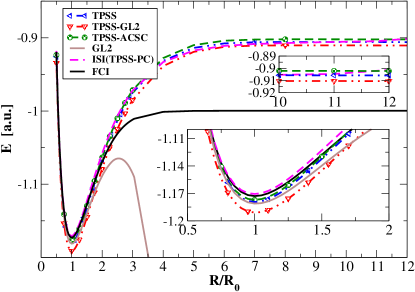
Figure 6: The total energy of the stretched H₂ molecule as it is calculated with the various methods. The insets present the same data around the equilibrium distance ($R/R_{0}=1$) and large $R/R_{0}>10$ values.

Let us focus on self-consistent results (@SCF) obtained within the generalized KS (gKS) scheme. As an example, we report in Tab. 5 AE6 Lynch and Truhlar (2003); Haunschild and Klopper (2012) atomization energies of $6$ small size molecules, obtained using SCF orbitals and densities. One can note that TPSS-ACSC functional, in general, gives results that are twice worse (MAE = 18.4 kcal/mol) than for the TPSS counterpart, which yields MAE of 7.6 kcal/mol. The same trend for the AE6 benchmark occurs when we feed TPSS-ACSC and TPSS total energy expressions with HF orbitals. This indicates the following things:

• The major part of the error for the TPSS-ACSC functional is related to functional-driven errorKim et al. (2013). This is most possibly related to the ACSC model itself, which was not designed to be accurate in the high-density limit where most of the chemical application takes place;

• because both TPSS and TPSS-ACSC utilize the same semi-local TPSS exchange, the larger error observed in the latter might suggest the lack of compatibility between exchange and correlation functionals (there is no error cancellation effect). The correlation energies are pretty accurate, as shown in Tab. 4. This might indicate that the correct behavior of TPSS-ACSC functional can be restored by proper design of compatible exchange functional;

To test this possibility, we have performed ad hoc modification of TPSS exchange functional Tao et al. (2003) by calibration of second-order gradient expansion parameter ($\mu=0.235$). We note that this parameter might generally vary based on the nature of the localized (such as atoms) or de-localized systems (solids). Using $\mu=0.40$, we have observed a significant reduction of MAE for AE6 obtained at @SCF densities to 6.63 kcal/mol.

Finally, the performance of the constructed functionals is also benchmarked for other molecular test cases such as atomization energies, barrier heights and week, and covalent interactions. These results are reported in Table 6. A noticeable improvement is observed from TPSS-ACSC ($\mu=0.40$) than TPSS-ACSC, especially for atomization energies. Interestingly, In other cases, TPSS-ACSC performs slightly better or similarly to TPSS-ACSC ($\mu=0.40$). This indicates that probably some more sophisticated modification of the TPSS exchange functional is required in order to improve the accuracy of the method for all benchmarked cases. One may note that for CT7, W17, and S22, we do not include the dispersion correction as including a functional-specific dispersion interaction is beyond the scope of the present paper.

Table 5: AE6 atomization energies (in kcal/mol) computed using self-consistent (@SCF) and Hartree-Fock (@HF) orbitals and densities, and TPSSx semi-local exchange and TPSS or TPSS-ACSC correlation functionals. The mean absolute error (MAE, in kcal/mol) is shown in the last row. The def2-QZVP basis set is used. All calculations are performed using Q-Chem code Shao et al. (2015).

	TPSS@SCF	TPSS-ACSC@SCF	TPSS-ACSC@SCF	Ref. Haunschild and Klopper (2012)
			($\mu=0.40$)
SiH4	334.2	337.9	332.0	323.1
SiO	187.1	189.4	179.3	191.5
S2	109.0	114.6	106.2	101.9
C3H4	707.8	724.0	699.8	701.0
C2H2O2	634.1	648.8	619.0	630.4
C4H8	1155.8	1182.8	1141.6	1143.4
MAE	7.6	18.4	6.6
	TPSS@HF	TPSS-ACSC@HF	TPSS-ACSC@HF	Ref. Haunschild and Klopper (2012)
			($\mu=0.40$)
SiH4	331.9	337.0	332.6	323.1
SiO	179.7	182.2	173.1	191.5
S2	103.5	109.5	101.5	101.9
C3H4	702.0	719.9	698.4	701.0
C2H2O2	621.1	637.2	610.3	630.4
C4H8	1148.3	1179.0	1142.8	1143.4
MAE	6.2	15.3	8.5

Table 6: Mean absolute errors (MAEs in kcal/mol) for the benchmark molecular tests, obtained using different methods. All calculations are performed self-consistently using a def2-QZVP basis set with Q-Chem code Shao et al. (2015).

	TPSS	TPSS-ACSC	TPSS-ACSC
			($\mu=0.40$)
G2/148a	5.5	15.7	7.8
BH6b	8.2	8.3	8.4
HTBH38c	7.7	8.3	7.1
NHTBH38c	9.2	9.2	9.1
CT7d	2.0	1.7	1.1
WI7d	0.24	0.26	0.12
S22e	3.4	4.1	5.5

^aatomization energies of 148 molecules Curtiss et al. (1997),^b 6 barrier heights Haunschild and Klopper (2012), ^c38 hydrogen (HTBH38) and 38 non-hydrogen bonded reaction barrier heights (NHTBH38) Zhao and Truhlar (2005a), ^d7 charge transfer molecules, and 7 weekly interacting test set Zhao and Truhlar (2005b), ^e22 non-covalent interacting systems Goerigk et al. (2017).

IV Conclusions

In this work, we have constructed a semilocal meta-GGA correlation energy functional, based on the ACSC method proposed in Refs. Constantin, 2019. The correlation functional, denoted as TPSS-ACSC, interpolates the high and low-density limit of the popular TPSS correlation energy functional showing some direction on how to incorporate a strong interaction regime within the approximate, semilocal exchange-correlation formula.

The new correlation TPSS-ACSC functional is non-empirical, one electron self-interaction free accurate for small atoms and molecules. We provide a careful assessment of TPSS-ACSC functional base on some model systems (the uniform electron gas, Hooke’s atom, stretched H₂ molecule) and real-life calculations (atomization energies) showing some advantages and disadvantages of ACSC construction. From this broad perspective, we can conclude that, although the ACSC method holds a promise for proper description of a strong-interaction regime, it is still in its infancy, which implies that there is still much space for improvement. The most important conclusions of the present study are as follows:

• the strong-interaction limit obtained from semilocal TPSS functional formula ($W_{\infty}^{TPSS}$ and $W_{\infty}^{{}^{\prime}TPSS}$) reproduce quite well reference SCE data. Moreover, both possess some other important features e.g., good performance in the quasi-2D regime and removing one electron self-interaction. Thus, both formulas could be effectively applied in constructing ACSC and ISI-like formulas.

• Although our numerical tests suggest the strong-interaction limit of semilocal TPSS-ACSC correlation is well represented, the semilocal GL2 part may need some amendment (Hooke’s atom, stretched H₂ molecule cases) e.g. via proper incorporation of local gap modelFabiano et al. (2014); Krieger et al. (1999); Constantin et al. (2017b).

• in order to improve the accuracy of TPSS-ACSC XC functional, it must be combined with the compatible exchange functional, leading to a much better balance in XC term (better mutual error cancelation effect). As was shown, the ad hoc modification of TPSS exchange gives some hints in that direction.

Some of these new developments in the ACSC context will be addressed in a future study.

Appendix A Details of TPSS-ACSC correlation functional

Here we summarized the expressions of energy density $w_{\alpha}$ of Eq. (4) $-$ Eq. (7) which is defined by $W_{\alpha}=\int~{}d^{3}r~{}w_{\alpha}(\bf{r})$. Thus one required following energy densities $w_{0}(\bf{r})$, $w_{0}^{\prime}(\bf{r})$, $w_{\infty}(\bf{r})$, and $w_{\infty}^{\prime}(\bf{r})$ to calculate the ACSC correlation.

We take in the following expressions:

(i) First, $w_{0}({\bf{r}})=n({\bf{r}})\epsilon_{x}^{TPSS}({\bf{r}})$, where $\epsilon_{x}^{TPSS}({\bf{r}}$ is the TPSS exchange energy per particle Tao et al. (2003) given by,

$$\epsilon_{x}^{TPSS}({\bf{r}})=-A_{x}n({\bf{r}})F_{x}^{TPSS},~{}F_{x}^{TPSS}=1+\kappa-\kappa/(1+x/\kappa)~{}$$ (12)

with $\kappa=0.804$. See ref. Tao et al. (2003) for the details of the TPSS exchange enhancement factor ($F_{x}^{TPSS}$).

(ii) Second, $w_{0}^{\prime}({\bf{r}})=2n({\bf{r}})\epsilon_{c}^{TPSS-GL2}$, where $\epsilon_{\mathrm{c}}^{\text{TPSS-GL2}}$ is the Görling-Levy second-order limit of the TPSS correlation energy Tao et al. (2003) per electron which is given by Perdew et al. (2008)

$$\epsilon_{\mathrm{c}}^{\text{TPSS-GL2}}=\epsilon_{\mathrm{c}}^{\text{revPKZB-GL2}}\left[1+d\epsilon_{\mathrm{c}}^{\text{revPKZB-GL2}}\left(\frac{\tau_{W}}{\tau}\right)^{3}\right],$$ (13)

where $d=2.8$ hartree^-1 is a constant and

$$\epsilon_{\mathrm{c}}^{\text{revPKZB-GL2}}$$

$$=\epsilon_{\mathrm{c}}^{\mathrm{PBE-GL2}}(n_{\uparrow},n_{\downarrow},\nabla n_{\uparrow},\nabla n_{\downarrow})\left[1+C(\zeta,\xi)\left(\frac{\tau_{W}}{\tau}\right)^{2}\right]$$

$$-\left[1+C(\zeta,\xi)\right]\left(\frac{\tau_{W}}{\tau}\right)^{2}\sum_{\sigma}\frac{n_{\sigma}}{n}\tilde{\epsilon}_{\mathrm{c,\sigma}}^{\mathrm{PBE-GL2}}.$$ (14)

In Eq. (14), $\epsilon_{\mathrm{c}}^{\text{PBE-GL2}}$ is the Görling–Levy limit of the PBE correlation energy per electron. It is obtained by replacing $\lambda\bf r$ with $\bf r$ in the $\lambda\to\infty$ uniform density scaling limit of the PBE correlation energy per electron, and has the expression

$$\epsilon_{\mathrm{c}}^{\text{PBE-GL2}}(n_{\uparrow},n_{\downarrow},\nabla n_{\uparrow},\nabla n_{\downarrow})$$

$$=-\gamma\phi^{3}\ln\left[1+\frac{1}{\chi s^{2}/\phi^{2}+(\chi s^{2}/\phi^{2})^{2}}\right]~{},$$ (15)

where $\gamma=(1-\ln 2)/\pi^{2}$, $\phi(\zeta)=\frac{1}{2}\left[(1+\zeta)^{2/3}+(1-\zeta)^{2/3}\right]$, $s=|\nabla n|/2nk_{F}$ is the reduced density gradient, $k_{F}=(3\pi^{2}n)^{1/3}$, and $\chi=(\beta/\gamma)c^{2}e^{-\omega/\gamma}\approx 0.72161$, where $c=(3\pi^{2}/16)^{1/3}$, $\beta=0.066725$, and $\omega=0.046644$.

The spin-dependent function $\tilde{\epsilon}_{\mathrm{c,\sigma}}^{\mathrm{PBE-GL2}}$ is defined as

$$\tilde{\epsilon}_{\mathrm{c,\sigma}}^{\mathrm{PBE-GL2}} = \max\big{[}\epsilon_{\mathrm{c}}^{\mathrm{PBE-GL2}}(n_{\sigma},0,\nabla n_{\sigma},0),$$ (16)

$$\epsilon_{\mathrm{c}}^{\mathrm{PBE-GL2}}(n_{\uparrow},n_{\downarrow},\nabla n_{\uparrow},\nabla n_{\downarrow})\big{]}.$$

The function $C(\zeta,\xi)$ is the spin-dependent function, where $\zeta$ is the spin-polarization and $\xi=|\nabla\zeta|/2k_{F}$.

(iii) Third, in the case of TPSS XC functional the $W_{\infty}$ is derived as,

$$W_{\infty}^{TPSS}[n_{\uparrow},n_{\downarrow}] = E_{x}^{TPSS}[n_{\uparrow},n_{\downarrow}]+\int~{}d^{3}r~{}n({\bf{r}})~{}\Big{\{}\Big{(}-\frac{d_{0}(\zeta)}{r_{s}}$$

$$+ H_{1}(r_{s},\zeta,t)\Big{)}\Big{[}1+C(\zeta,\xi)\Big{(}\frac{\tau^{W}}{\tau}\Big{)}^{2}\Big{]}$$

$$- (1+C(\zeta,\xi))\Big{(}\frac{\tau^{W}}{\tau}\Big{)}^{2}\sum_{\sigma}\frac{n_{\sigma}}{n}\Big{(}-\frac{d_{0}(1)}{r_{s,\sigma}}$$

$$+ H_{1}(r_{s,\sigma},1,t_{\sigma})\Big{)}\Big{\}}$$

(iv) Fourth and finally, $W^{\prime}_{\infty}$ for TPSS functional reads

$$W_{\infty}^{{}^{\prime}TPSS}[n_{\uparrow},n_{\downarrow}] = \frac{1}{2}\int~{}d^{3}r~{}n({\bf{r}})~{}\Big{\{}\Big{(}\frac{d_{1}(\zeta)}{r_{s}^{3/2}}$$

$$+ H_{2}(r_{s},\zeta,t)\Big{)}\Big{[}1+C(\zeta,\xi)\Big{(}\frac{\tau^{W}}{\tau}\Big{)}^{2}\Big{]}$$

$$- (1+C(\zeta,\xi))\Big{(}\frac{\tau^{W}}{\tau}\Big{)}^{2}\sum_{\sigma}\frac{n_{\sigma}}{n}\Big{(}\frac{d_{1}(1)}{r_{s,\sigma}^{3/2}}$$

$$+ H_{2}(r_{s,\sigma},1,t_{\sigma})\Big{)}\Big{\}}~{},$$

where $d_{1}(\zeta)=1.5$ (spin-independent) was fixed using the same reasoning as in Refs. Seidl et al., 2000b and $E_{x}^{TPSS}[n_{\uparrow},n_{\downarrow}]$ is the spin-resolved TPSS exchange Tao et al. (2003). $H_{1}$ and $H_{2}$ are same as given by Eq. (D11) and Eq. (D12) of Refs. Seidl et al., 2000b. $C(\zeta,\xi)$ is given in Eq. (14) of Refs. Tao et al., 2003. We recall that $W_{\infty}^{TPSS}[n_{\uparrow},n_{\downarrow}]$ was already reported in Refs. Perdew et al., 2004. However, the expression of $W_{\infty}^{{}^{\prime}TPSS}[n_{\uparrow},n_{\downarrow}]$ can be obtained in the similar fashion as Eq. (D16) of PKZB expression Seidl et al. (2000b). For the details of the parameters and terms see Refs. Seidl et al., 2000b (for $d_{0}(\zeta)$, $d_{1}(\zeta)$, and $d_{1}(1)$) and Refs. Tao et al., 2003 (for $C(\zeta,\xi)$). One may note that the expressions of TPSS (given in this paper) differ from PKZB (given in Refs. Seidl et al., 2000b) from their correlation point of view. Note that Eq. LABEL:err1 is slightly different from Eq.(38) of ref. Perdew et al. (2004). Similarly, Eq. LABEL:eer is constructed to ensure its’ becomes positive.

References

- Kohn and Sham (1965) W. Kohn and L. J. Sham, Phys. Rev. 140, A1133 (1965).
- Hohenberg and Kohn (1964) P. Hohenberg and W. Kohn, Phys. Rev. 136, B864 (1964).
- Burke (2012) K. Burke, J. Chem. Phys. 136, 150901 (2012).
- Levy (2010) M. Levy, International Journal of Quantum Chemistry 110, 3140 (2010).
- Levy (2016) M. Levy, Int. J. Quantum Chem. 116, 802 (2016).
- Sun et al. (2015) J. Sun, A. Ruzsinszky, and J. P. Perdew, Phys. Rev. Lett. 115, 036402 (2015).
- Tao and Mo (2016) J. Tao and Y. Mo, Phys. Rev. Lett. 117, 073001 (2016).
- Levy and Perdew (1985) M. Levy and J. P. Perdew, Phys. Rev. A 32, 2010 (1985).
- Görling and Levy (1992) A. Görling and M. Levy, Phys. Rev. A 45, 1509 (1992).
- Fabiano and Constantin (2013) E. Fabiano and L. A. Constantin, Phys. Rev. A 87, 012511 (2013).
- Svendsen and von Barth (1996) P.-S. Svendsen and U. von Barth, Phys. Rev. B 54, 17402 (1996).
- Antoniewicz and Kleinman (1985) P. R. Antoniewicz and L. Kleinman, Phys. Rev. B 31, 6779 (1985).
- Hu and Langreth (1986) C. D. Hu and D. C. Langreth, Phys. Rev. B 33, 943 (1986).
- Ma and Brueckner (1968) S.-K. Ma and K. A. Brueckner, Phys. Rev. 165, 18 (1968).
- Argaman et al. (2022) N. Argaman, J. Redd, A. C. Cancio, and K. Burke, Phys. Rev. Lett. 129, 153001 (2022).
- Daas et al. (2022a) T. J. Daas, D. P. Kooi, A. J. A. F. Grooteman, M. Seidl, and P. Gori-Giorgi, Journal of Chemical Theory and Computation 18, 1584 (2022a).
- Daas et al. (2022b) T. J. Daas, D. P. Kooi, T. Benyahia, M. Seidl, and P. Gori-Giorgi, (2022b), arXiv:2211.07512 [physics.chem-ph] .
- Görling and Levy (1994) A. Görling and M. Levy, Phys. Rev. A 50, 196 (1994).
- Görling and Levy (1993) A. Görling and M. Levy, Phys. Rev. B 47, 13105 (1993).
- Görling and Levy (1995) A. Görling and M. Levy, Phys. Rev. A 52, 4493 (1995).
- Della Sala and Görling (2002) F. Della Sala and A. Görling, Phys. Rev. Lett. 89, 033003 (2002).
- Engel et al. (1992) E. Engel, J. Chevary, L. Macdonald, and S. Vosko, Z. Phys. D 23, 7 (1992).
- Horowitz et al. (2009) C. M. Horowitz, L. A. Constantin, C. R. Proetto, and J. M. Pitarke, Phys. Rev. B 80, 235101 (2009).
- Constantin and Pitarke (2011) L. A. Constantin and J. M. Pitarke, Physical Review B 83, 075116 (2011).
- Constantin et al. (2016a) L. A. Constantin, E. Fabiano, J. M. Pitarke, and F. Della Sala, Phys. Rev. B 93, 115127 (2016a).
- Niquet et al. (2003) Y. M. Niquet, M. Fuchs, and X. Gonze, J. Chem. Phys. 118, 9504 (2003).
- Almbladh and von Barth (1985) C.-O. Almbladh and U. von Barth, Phys. Rev. B 31, 3231 (1985).
- Umrigar and Gonze (1994) C. J. Umrigar and X. Gonze, Phys. Rev. A 50, 3827 (1994).
- Pollack and Perdew (2000) L. Pollack and J. Perdew, Journal of Physics: Condensed Matter 12, 1239 (2000).
- Kaplan et al. (2018) A. D. Kaplan, K. Wagle, and J. P. Perdew, Phys. Rev. B 98, 085147 (2018).
- Constantin (2016) L. A. Constantin, Phys. Rev. B 93, 121104 (2016).
- Constantin (2008) L. A. Constantin, Phys. Rev. B 78, 155106 (2008).
- Tao et al. (2008) J. Tao, V. N. Staroverov, G. E. Scuseria, and J. P. Perdew, Phys. Rev. A 77, 012509 (2008).
- Přecechtělová et al. (2014) J. Přecechtělová, H. Bahmann, M. Kaupp, and M. Ernzerhof, J. Chem. Phys. 141, 111102 (2014).
- Přecechtělová et al. (2015) J. P. Přecechtělová, H. Bahmann, M. Kaupp, and M. Ernzerhof, J. Chem. Phys. 143, 144102 (2015).
- Perdew and Schmidt (2001) J. P. Perdew and K. Schmidt, in AIP Conference Proceedings (IOP INSTITUTE OF PHYSICS PUBLISHING LTD, 2001) pp. 1–20.
- Grimme (2006) S. Grimme, J. Chem. Phys. 124, 034108 (2006), https://doi.org/10.1063/1.2148954 .
- Mehta et al. (2018) N. Mehta, M. Casanova-Páez, and L. Goerigk, Phys. Chem. Chem. Phys. 20, 23175 (2018).
- Bartlett et al. (2005a) R. J. Bartlett, I. Grabowski, S. Hirata, and S. Ivanov, J. Chem. Phys. 122, 034104 (2005a).
- Grabowski et al. (2014) I. Grabowski, E. Fabiano, A. M. Teale, S. Śmiga, A. Buksztel, and F. D. Sala, J. Chem. Phys. 141, 024113 (2014).
- Śmiga et al. (2020) S. Śmiga, V. Marusiak, I. Grabowski, and E. Fabiano, J. Chem. Phys. 152, 054109 (2020).
- Siecińska et al. (2022) S. Siecińska, S. Śmiga, I. Grabowski, F. D. Sala, and E. Fabiano, Molecular Physics 0, e2037771 (2022), https://doi.org/10.1080/00268976.2022.2037771 .
- Seidl et al. (2000a) M. Seidl, J. P. Perdew, and S. Kurth, Phys. Rev. Lett. 84, 5070 (2000a).
- Perdew et al. (1996a) J. P. Perdew, K. Burke, and M. Ernzerhof, Phys. Rev. Lett. 77, 3865 (1996a).
- Scuseria and Staroverov (2005) G. E. Scuseria and V. N. Staroverov, in Theory and Application of Computational Chemistry: The First 40 Years, edited by C. E. Dykstra, G. Frenking, K. S. Kim, and G. E. Scuseria (Elsevier: Amsterdam, 2005) pp. 669–724.
- Tao et al. (2003) J. Tao, J. P. Perdew, V. N. Staroverov, and G. E. Scuseria, Phys. Rev. Lett. 91, 146401 (2003).
- Jana et al. (2019a) S. Jana, K. Sharma, and P. Samal, The Journal of Physical Chemistry A 123, 6356 (2019a).
- Patra et al. (2019) B. Patra, S. Jana, L. A. Constantin, and P. Samal, Phys. Rev. B 100, 155140 (2019).
- Jana et al. (2021a) S. Jana, S. K. Behera, S. Śmiga, L. A. Constantin, and P. Samal, New J. Phys. 23, 063007 (2021a).
- Patra et al. (2020) A. Patra, S. Jana, and P. Samal, The Journal of Chemical Physics 153, 184112 (2020), https://doi.org/10.1063/5.0025173 .
- Jana et al. (2021b) S. Jana, S. K. Behera, S. Śmiga, L. A. Constantin, and P. Samal, The Journal of Chemical Physics 155, 024103 (2021b), https://doi.org/10.1063/5.0051331 .
- Janesko and Aguero (2012) B. G. Janesko and A. Aguero, J. Chem. Phys. 136, 024111 (2012).
- Janesko (2013) B. G. Janesko, Int. J. Quantum Chem. 113, 83 (2013).
- Janesko (2010) B. G. Janesko, J. Chem. Phys. 133, 104103 (2010).
- Janesko (2012) B. G. Janesko, J. Chem. Phys. 137, 224110 (2012).
- Janesko et al. (2018) B. G. Janesko, E. Proynov, G. Scalmani, and M. J. Frisch, J. Chem. Phys. 148, 104112 (2018).
- Constantin et al. (2016b) L. A. Constantin, E. Fabiano, and F. Della Sala, J. Chem. Phys. 145, 084110 (2016b).
- Constantin et al. (2017a) L. A. Constantin, E. Fabiano, and F. Della Sala, J. Chem. Theory Comput. 13, 4228 (2017a).
- Perdew et al. (2008) J. P. Perdew, V. N. Staroverov, J. Tao, and G. E. Scuseria, Phys. Rev. A 78, 052513 (2008).
- Perdew et al. (2005) J. P. Perdew, A. Ruzsinszky, J. Tao, V. N. Staroverov, G. E. Scuseria, and G. I. Csonka, J. Chem. Phys. 123, 062201 (2005).
- Odashima and Capelle (2009) M. M. Odashima and K. Capelle, Phys. Rev. A 79, 062515 (2009).
- Arbuznikov and Kaupp (2011) A. V. Arbuznikov and M. Kaupp, Int. J. Quantum Chem. 111, 2625 (2011).
- Jaramillo et al. (2003) J. Jaramillo, G. E. Scuseria, and M. Ernzerhof, J. Chem. Phys. 118, 1068 (2003).
- Kümmel and Kronik (2008) S. Kümmel and L. Kronik, Reviews of Modern Physics 80, 3 (2008).
- Becke (2005) A. D. Becke, J. Chem. Phys. 122, 064101 (2005).
- Becke and Johnson (2007) A. D. Becke and E. R. Johnson, J. Chem. Phys. 127, 124108 (2007).
- Becke (2003) A. D. Becke, J. Chem. Phys. 119, 2972 (2003).
- Becke (2013) A. D. Becke, J. Chem. Phys. 138, 074109 (2013).
- Patra et al. (2018) B. Patra, S. Jana, and P. Samal, Phys. Chem. Chem. Phys. 20, 8991 (2018).
- Jana et al. (2018a) S. Jana, A. Patra, and P. Samal, The Journal of Chemical Physics 149, 094105 (2018a).
- Jana and Samal (2019) S. Jana and P. Samal, Phys. Chem. Chem. Phys. 21, 3002 (2019).
- Jana et al. (2018b) S. Jana, B. Patra, H. Myneni, and P. Samal, Chemical Physics Letters 713, 1 (2018b).
- Jana et al. (2020a) S. Jana, A. Patra, L. A. Constantin, and P. Samal, The Journal of Chemical Physics 152, 044111 (2020a).
- Jana et al. (2019b) S. Jana, A. Patra, L. A. Constantin, H. Myneni, and P. Samal, Phys. Rev. A 99, 042515 (2019b).
- Jana et al. (2022) S. Jana, L. A. Constantin, S. Śmiga, and P. Samal, The Journal of Chemical Physics 157, 024102 (2022).
- Grimme and Neese (2007) S. Grimme and F. Neese, The Journal of Chemical Physics 127, 154116 (2007).
- Su and Xu (2014) N. Q. Su and X. Xu, The Journal of Chemical Physics 140, 18A512 (2014), https://doi.org/10.1063/1.4866457 .
- Hui and Chai (2016) K. Hui and J.-D. Chai, The Journal of Chemical Physics 144, 044114 (2016).
- Sharkas et al. (2011) K. Sharkas, J. Toulouse, and A. Savin, The Journal of chemical physics 134, 064113 (2011).
- Souvi et al. (2014) S. M. Souvi, K. Sharkas, and J. Toulouse, The Journal of chemical physics 140, 084107 (2014).
- Toulouse et al. (2011) J. Toulouse, K. Sharkas, E. Brémond, and C. Adamo, The Journal of Chemical Physics 135, 101102 (2011), https://doi.org/10.1063/1.3640019 .
- Toulouse et al. (2009) J. Toulouse, I. C. Gerber, G. Jansen, A. Savin, and J. G. Angyán, Phys. Rev. Lett. 102, 096404 (2009).
- Ruzsinszky et al. (2016) A. Ruzsinszky, L. A. Constantin, and J. M. Pitarke, Phys. Rev. B 94, 165155 (2016).
- Ruzsinszky et al. (2010) A. Ruzsinszky, J. P. Perdew, and G. I. Csonka, Journal of Chemical Theory and Computation 6, 127 (2010).
- Bates et al. (2017) J. E. Bates, J. Sensenig, and A. Ruzsinszky, Phys. Rev. B 95, 195158 (2017).
- Terentjev et al. (2018) A. V. Terentjev, L. A. Constantin, and J. M. Pitarke, Phys. Rev. B 98, 085123 (2018).
- Corradini et al. (1998) M. Corradini, R. Del Sole, G. Onida, and M. Palummo, Phys. Rev. B 57, 14569 (1998).
- Erhard et al. (2016) J. Erhard, P. Bleiziffer, and A. Görling, Phys. Rev. Lett. 117, 143002 (2016).
- Patrick and Thygesen (2015) C. E. Patrick and K. S. Thygesen, J. Chem. Phys. 143, 102802 (2015).
- Bartlett et al. (2005b) R. J. Bartlett, I. Grabowski, S. Hirata, and S. Ivanov, J. Chem. Phys. 122, 034104 (2005b).
- Bartlett et al. (2005c) R. J. Bartlett, V. F. Lotrich, and I. V. Schweigert, J. Chem. Phys. 123, 062205 (2005c).
- Grabowski et al. (2013) I. Grabowski, E. Fabiano, and F. Della Sala, Phys. Rev. B 87, 075103 (2013).
- Langreth and Perdew (1975) D. C. Langreth and J. P. Perdew, Solid State Communications 17, 1425 (1975).
- Gunnarsson and Lundqvist (1976) O. Gunnarsson and B. I. Lundqvist, Phys. Rev. B 13, 4274 (1976).
- Savin et al. (2003) A. Savin, F. Colonna, and R. Pollet, Int. J. Quantum Chem. 93, 166 (2003).
- Cohen et al. (2007) A. J. Cohen, P. Mori-Sánchez, and W. Yang, J. Chem. Phys. 127, 034101 (2007).
- Ernzerhof (1996) M. Ernzerhof, Chem. Phys. Lett. 263, 499 (1996).
- Burke et al. (1997) K. Burke, M. Ernzerhof, and J. P. Perdew, Chem. Phys. Lett. 265, 115 (1997).
- Colonna and Savin (1999) F. Colonna and A. Savin, J. Chem. Phys. 110, 2828 (1999).
- Adamo and Barone (1998) C. Adamo and V. Barone, J. Chem. Phys. 108, 664 (1998).
- Perdew et al. (2001) J. P. Perdew, S. Kurth, and M. Seidl, Int. J. Mod. Phys. B 15, 1672 (2001).
- Liu and Burke (2009) Z.-F. Liu and K. Burke, Phys. Rev. A 79, 064503 (2009).
- Magyar et al. (2003) R. Magyar, W. Terilla, and K. Burke, J. Chem. Phys. 119, 696 (2003).
- Sun (2009) J. Sun, J. Chem. Theory Comput. 5, 708 (2009).
- Seidl and Gori-Giorgi (2010) M. Seidl and P. Gori-Giorgi, Phys. Rev. A 81, 012508 (2010).
- Vuckovic et al. (2016a) S. Vuckovic, T. J. Irons, A. Savin, A. M. Teale, and P. Gori-Giorgi, J. Chem. Theory Comput. 12, 2598 (2016a).
- Fabiano et al. (2019) E. Fabiano, S. Śmiga, S. Giarrusso, T. J. Daas, F. Della Sala, I. Grabowski, and P. Gori-Giorgi, Journal of Chemical Theory and Computation 15, 1006 (2019), https://doi.org/10.1021/acs.jctc.8b01037 .
- Vuckovic et al. (2018) S. Vuckovic, P. Gori-Giorgi, F. Della Sala, and E. Fabiano, The Journal of Physical Chemistry Letters 9, 3137 (2018), pMID: 29787273, https://doi.org/10.1021/acs.jpclett.8b01054 .
- Kooi and Gori-Giorgi (2018) D. P. Kooi and P. Gori-Giorgi, Theor. Chem. Acc. 137, 166 (2018).
- Seidl et al. (2018) M. Seidl, S. Giarrusso, S. Vuckovic, E. Fabiano, and P. Gori-Giorgi, J. Chem. Phys. 149, 241101 (2018).
- Constantin (2019) L. A. Constantin, Phys. Rev. B 99, 085117 (2019).
- Görling (1998) A. Görling, Int. J. Quantum Chem. 69, 265 (1998).
- Seidl et al. (2000b) M. Seidl, J. P. Perdew, and S. Kurth, Phys. Rev. A 62, 012502 (2000b).
- Gori-Giorgi et al. (2009a) P. Gori-Giorgi, G. Vignale, and M. Seidl, J. Chem. Theory Comput. 5, 743 (2009a).
- Seidl et al. (2007) M. Seidl, P. Gori-Giorgi, and A. Savin, Phys. Rev. A 75, 042511 (2007).
- Gori-Giorgi et al. (2009b) P. Gori-Giorgi, G. Vignale, and M. Seidl, J. Chem. Theory Comput. 5, 743 (2009b).
- Malet et al. (2013) F. Malet, A. Mirtschink, J. C. Cremon, S. M. Reimann, and P. Gori-Giorgi, Phys. Rev. B 87, 115146 (2013).
- Gori-Giorgi and Seidl (2010) P. Gori-Giorgi and M. Seidl, Phys. Chem. Chem. Phys. 12, 14405 (2010).
- Fabiano et al. (2016) E. Fabiano, P. Gori-Giorgi, M. Seidl, and F. Della Sala, J. Chem. Theory Comput. 12, 4885 (2016).
- Seidl et al. (1999a) M. Seidl, J. P. Perdew, and M. Levy, Phys. Rev. A 59, 51 (1999a).
- Seidl et al. (2016) M. Seidl, S. Vuckovic, and P. Gori-Giorgi, Mol. Phys. 114, 1076 (2016).
- Giarrusso et al. (2018) S. Giarrusso, P. Gori-Giorgi, F. Della Sala, and E. Fabiano, J. Chem. Phys. 148, 134106 (2018).
- Mirtschink et al. (2012) A. Mirtschink, M. Seidl, and P. Gori-Giorgi, J. Chem. Theory Comput. 8, 3097 (2012).
- Seidl et al. (1999b) M. Seidl, J. P. Perdew, and M. Levy, Phys. Rev. A 59, 51 (1999b).
- Daas et al. (2021) T. J. Daas, E. Fabiano, F. Della Sala, P. Gori-Giorgi, and S. Vuckovic, The Journal of Physical Chemistry Letters 12, 4867 (2021), pMID: 34003655, https://doi.org/10.1021/acs.jpclett.1c01157 .
- Śmiga et al. (2022) S. Śmiga, F. Della Sala, P. Gori-Giorgi, and E. Fabiano, Journal of Chemical Theory and Computation 18, 5936 (2022), pMID: 36094908, https://doi.org/10.1021/acs.jctc.2c00352 .
- Vuckovic et al. (2016b) S. Vuckovic, T. J. P. Irons, A. Savin, A. M. Teale, and P. Gori-Giorgi, Journal of Chemical Theory and Computation 12, 2598 (2016b), pMID: 27116427, https://doi.org/10.1021/acs.jctc.6b00177 .
- Śmiga et al. (2017) S. Śmiga, E. Fabiano, L. A. Constantin, and F. Della Sala, The Journal of chemical physics 146, 064105 (2017).
- Perdew et al. (1996b) J. P. Perdew, K. Burke, and Y. Wang, Phys. Rev. B 54, 16533 (1996b).
- Śmiga and Constantin (2020) S. Śmiga and L. A. Constantin, J. Chem. Theory Comput. 16, 4983 (2020).
- Perdew et al. (2004) J. P. Perdew, J. Tao, V. N. Staroverov, and G. E. Scuseria, J. Chem. Phys. 120, 6898 (2004).
- von Weizsäcker (1935) C. F. von Weizsäcker, Zeitschrift für Physik A Hadrons and Nuclei 96, 431 (1935).
- Della Sala et al. (2015) F. Della Sala, E. Fabiano, and L. A. Constantin, Phys. Rev. B 91, 035126 (2015).
- Perdew and Wang (1992) J. P. Perdew and Y. Wang, Phys. Rev. B 45, 13244 (1992).
- Lee et al. (1988) C. Lee, W. Yang, and R. G. Parr, Phys. Rev. B 37, 785 (1988).
- Fabiano et al. (2015) E. Fabiano, L. Constantin, A. Terentjevs, F. Della Sala, and P. Cortona, Theor. Chem. Acc. 134, 139 (2015).
- Tognetti et al. (2008) V. Tognetti, P. Cortona, and C. Adamo, The Journal of chemical physics 128, 034101 (2008).
- Ragot and Cortona (2004) S. Ragot and P. Cortona, The Journal of chemical physics 121, 7671 (2004).
- Daas et al. (2022c) T. J. Daas, D. P. Kooi, T. Benyahia, M. Seidl, and P. Gori-Giorgi, “Large-z atoms in the strong-interaction limit of dft: Implications for gradient expansions and for the lieb-oxford bound,” (2022c), arXiv:2211.07512 .
- Perdew et al. (2014) J. P. Perdew, A. Ruzsinszky, J. Sun, and K. Burke, J. Chem. Phys. 140, 18A533 (2014).
- Taut (1993) M. Taut, Phys. Rev. A 48, 3561 (1993).
- Davidson et al. (1991) E. R. Davidson, S. A. Hagstrom, S. J. Chakravorty, V. M. Umar, and C. F. Fischer, Phys. Rev. A 44, 7071 (1991).
- Chakravorty et al. (1993) S. J. Chakravorty, S. R. Gwaltney, E. R. Davidson, F. A. Parpia, and C. F. Fischer, Phys. Rev. A 47, 3649 (1993).
- Clementi and Corongiu (1997) E. Clementi and G. Corongiu, Int. J. Quantum Chem. 62, 571 (1997).
- Dunning (1989) T. H. Dunning, J. Chem. Phys. 90, 1007 (1989).
- Clementi and Roetti (1974) E. Clementi and C. Roetti, Atomic data and nuclear data tables 14, 177 (1974).
- Stanton et al. (2007) J. F. Stanton, J. Gauss, J. D. Watts, M. Nooijen, N. Oliphant, S. A. Perera, P. Szalay, W. J. Lauderdale, S. Kucharski, S. Gwaltney, S. Beck, A. Balková, D. E. Bernholdt, K. K. Baeck, P. Rozyczko, H. Sekino, C. Hober, and R. J. Bartlett Integral packages included are VMOL (J. Almlöf and P.R. Taylor); VPROPS (P. Taylor) ABACUS; (T. Helgaker, H.J. Aa. Jensen, P. Jörgensen, J. Olsen, and P.R. Taylor), ACES II (Quantum Theory Project, Gainesville, Florida, 2007).
- Kim et al. (2013) M.-C. Kim, E. Sim, and K. Burke, Phys. Rev. Lett. 111, 073003 (2013).
- Hernandez et al. (2023) D. J. Hernandez, A. Rettig, and M. Head-Gordon, arXiv preprint arXiv:2306.15016 (2023).
- Jana et al. (2020b) S. Jana, B. Patra, S. Śmiga, L. A. Constantin, and P. Samal, Phys. Rev. B 102, 155107 (2020b).
- Cohen et al. (2012) A. J. Cohen, P. Mori-Sánchez, and W. Yang, Chem. Rev. 112, 289–320 (2012), https://doi.org/10.1021/cr200107z .
- Kirkpatrick et al. (2021) J. Kirkpatrick, B. McMorrow, D. H. P. Turban, A. L. Gaunt, J. S. Spencer, A. G. D. G. Matthews, A. Obika, L. Thiry, M. Fortunato, D. Pfau, L. R. Castellanos, S. Petersen, A. W. R. Nelson, P. Kohli, P. Mori-Sánchez, D. Hassabis, and A. J. Cohen, Science 374, 1385–1389 (2021), https://www.science.org/doi/pdf/10.1126/science.abj6511 .
- Peach et al. (2007) M. J. G. Peach, A. M. Teale, and D. J. Tozer, The Journal of Chemical Physics 126, 244104 (2007).
- Fabiano et al. (2014) E. Fabiano, P. E. Trevisanutto, A. Terentjevs, and L. A. Constantin, J. Chem. Theory Comput. 10, 2016 (2014).
- Krieger et al. (1999) J. Krieger, J. Chen, G. Iafrate, A. Savin, A. Gonis, and N. Kioussis, Kluwer Academic, New York , 463 (1999).
- Constantin et al. (2017b) L. A. Constantin, E. Fabiano, S. Śmiga, and F. Della Sala, Phys. Rev. B 95, 115153 (2017b).
- Matito et al. (2010) E. Matito, J. Cioslowski, and S. F. Vyboishchikov, Phys. Chem. Chem. Phys. 12, 6712 (2010).
- Lynch and Truhlar (2003) B. J. Lynch and D. G. Truhlar, J. Phys. Chem. A 107, 8996 (2003).
- Haunschild and Klopper (2012) R. Haunschild and W. Klopper, Theor. Chem. Acc. 131, 1112 (2012).
- Shao et al. (2015) Y. Shao, Z. Gan, E. Epifanovsky, A. T. Gilbert, M. Wormit, J. Kussmann, A. W. Lange, A. Behn, J. Deng, X. Feng, D. Ghosh, M. Goldey, P. R. Horn, L. D. Jacobson, I. Kaliman, R. Z. Khaliullin, T. Kuś, A. Landau, J. Liu, E. I. Proynov, Y. M. Rhee, R. M. Richard, M. A. Rohrdanz, R. P. Steele, E. J. Sundstrom, H. L. W. III, P. M. Zimmerman, D. Zuev, B. Albrecht, E. Alguire, B. Austin, G. J. O. Beran, Y. A. Bernard, E. Berquist, K. Brandhorst, K. B. Bravaya, S. T. Brown, D. Casanova, C.-M. Chang, Y. Chen, S. H. Chien, K. D. Closser, D. L. Crittenden, M. Diedenhofen, R. A. D. Jr., H. Do, A. D. Dutoi, R. G. Edgar, S. Fatehi, L. Fusti-Molnar, A. Ghysels, A. Golubeva-Zadorozhnaya, J. Gomes, M. W. Hanson-Heine, P. H. Harbach, A. W. Hauser, E. G. Hohenstein, Z. C. Holden, T.-C. Jagau, H. Ji, B. Kaduk, K. Khistyaev, J. Kim, J. Kim, R. A. King, P. Klunzinger, D. Kosenkov, T. Kowalczyk, C. M. Krauter, K. U. Lao, A. D. Laurent, K. V. Lawler, S. V. Levchenko, C. Y. Lin, F. Liu, E. Livshits, R. C. Lochan, A. Luenser, P. Manohar, S. F. Manzer, S.-P. Mao, N. Mardirossian, A. V. Marenich, S. A. Maurer, N. J. Mayhall, E. Neuscamman, C. M. Oana, R. Olivares-Amaya, D. P. O’Neill, J. A. Parkhill, T. M. Perrine, R. Peverati, A. Prociuk, D. R. Rehn, E. Rosta, N. J. Russ, S. M. Sharada, S. Sharma, D. W. Small, A. Sodt, T. Stein, D. Stück, Y.-C. Su, A. J. Thom, T. Tsuchimochi, V. Vanovschi, L. Vogt, O. Vydrov, T. Wang, M. A. Watson, J. Wenzel, A. White, C. F. Williams, J. Yang, S. Yeganeh, S. R. Yost, Z.-Q. You, I. Y. Zhang, X. Zhang, Y. Zhao, B. R. Brooks, G. K. Chan, D. M. Chipman, C. J. Cramer, W. A. G. III, M. S. Gordon, W. J. Hehre, A. Klamt, H. F. S. III, M. W. Schmidt, C. D. Sherrill, D. G. Truhlar, A. Warshel, X. Xu, A. Aspuru-Guzik, R. Baer, A. T. Bell, N. A. Besley, J.-D. Chai, A. Dreuw, B. D. Dunietz, T. R. Furlani, S. R. Gwaltney, C.-P. Hsu, Y. Jung, J. Kong, D. S. Lambrecht, W. Liang, C. Ochsenfeld, V. A. Rassolov, L. V. Slipchenko, J. E. Subotnik, T. V. Voorhis, J. M. Herbert, A. I. Krylov, P. M. Gill, and M. Head-Gordon, Molecular Physics 113, 184 (2015).
- Curtiss et al. (1997) L. A. Curtiss, K. Raghavachari, P. C. Redfern, and J. A. Pople, The Journal of Chemical Physics 106, 1063 (1997).
- Zhao and Truhlar (2005a) Y. Zhao and D. G. Truhlar, Journal of Chemical Theory and Computation 1, 415 (2005a).
- Zhao and Truhlar (2005b) Y. Zhao and D. G. Truhlar, The Journal of Physical Chemistry A 109, 5656 (2005b).
- Goerigk et al. (2017) L. Goerigk, A. Hansen, C. Bauer, S. Ehrlich, A. Najibi, and S. Grimme, Phys. Chem. Chem. Phys. 19, 32184 (2017).