babble: Learning Better Abstractions with E-Graphs and Anti-Unification

Abstract.

Library learning compresses a given corpus of programs by extracting common structure from the corpus into reusable library functions. Prior work on library learning suffers from two limitations that prevent it from scaling to larger, more complex inputs. First, it explores too many candidate library functions that are not useful for compression. Second, it is not robust to syntactic variation in the input.

We propose library learning modulo theory (LLMT), a new library learning algorithm that additionally takes as input an equational theory for a given problem domain. LLMT uses e-graphs and equality saturation to compactly represent the space of programs equivalent modulo the theory, and uses a novel e-graph anti-unification technique to find common patterns in the corpus more directly and efficiently.

We implemented LLMT in a tool named babble. Our evaluation shows that babble achieves better compression orders of magnitude faster than the state of the art. We also provide a qualitative evaluation showing that babble learns reusable functions on inputs previously out of reach for library learning.

1. Introduction

Abstraction is the key to managing software complexity. Experienced programmers routinely extract common functionality into libraries of reusable abstractions to express their intent more clearly and concisely. What if this process of extracting useful abstractions from code could be automated? Library learning seeks to answer this question with techniques to compress a given corpus of programs by extracting common structure into reusable library functions. Library learning has many potential applications from refactoring and decompilation (Nandi et al., 2020; Jones et al., 2021), to modeling human cognition (Wang et al., 2021; Wong et al., 2022), and speeding up program synthesis by specializing the target language to a chosen problem domain (Ellis et al., 2021).

Consider the simple library learning task in Fig. 1. On the left, Fig. 1a shows a corpus of three programs in a 2d cad DSL from Wong et al. (2022). Each program corresponds to a picture composed of regular polygons, each of which is made of multiple rotated line segments. On the right, Fig. 1b shows a learned library with a single function (named f0) that abstracts away the construction of scaled regular polygons. The three input programs can then be refactored into a more concise form using the learned f0. Whether f0 is the “best” abstraction for this corpus is generally hard to quantify. For this paper, we follow DreamCoder (Ellis et al., 2021) and use compression as a metric for library learning, i.e., the goal is to reduce the total size of the corpus in AST nodes (from 208 to 72 Fig. 1). Importantly, the total size of the corpus includes the size of the library: this prevents library learning from generating too many overly-specific functions, and instead biases it towards more general and reusable abstractions.

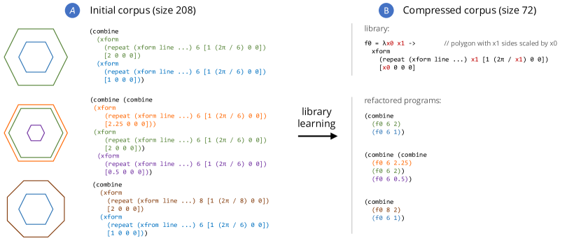
Figure 1. Example of library learning. Initial corpus A contains three graphical programs from the “nuts & bolts” dataset of Wong et al. (2022). Corpus B is the output of library learning with a single learned function for a scaled polygon, and the original programs refactored using this function.

Library learning can be phrased as a program synthesis problem structured in two phases: generating candidate abstractions, and then selecting those abstractions that produce the best (smallest) refactored corpus. The state-of-the-art technique, implemented in DreamCoder (Ellis et al., 2021), suffers from two primary limitations that hinder scaling library learning to larger and more realistic inputs.

• Candidate generation is not precise: DreamCoder generates many candidate abstractions that cannot be useful, slowing down the selection phase and the algorithm as a whole.

• The technique is purely syntactic and hence not robust to superficial variation. For example, a human programmer would immediately know that the terms $2+1$ and $1+3$ can be refactored using the abstraction $\lambda x\ \mathbf{\shortrightarrow}\ x+1$, because addition commutes; a purely syntactic library learning approach cannot generate this abstraction.

In this paper we propose library learning modulo (equational) theories (LLMT)—a new library learning algorithm that addresses both of the above limitations.

Precise Candidate Generation via Anti-Unification. To make candidate generation more precise, LLMT leverages two key observations:

• Useful abstractions must be used in the corpus at least twice. For example, in a corpus of two programs $2+1$ and $3+1$, there is no need to consider $\lambda x\ \mathbf{\shortrightarrow}\ 3+x$ because it can only be used in one place, and hence would only increase the size of the corpus.

• Abstractions should be “as concrete as possible” for a given corpus. For example, in the same corpus with $2+1$ and $3+1$, the abstraction $\lambda x\ \mathbf{\shortrightarrow}\ x+1$ is superior to the more general $\lambda x\ y\ \mathbf{\shortrightarrow}\ x+y$, since both apply to the same two terms, but applying the latter is more expensive (it requires two arguments).

In other words, a useful abstraction corresponds to the least general pattern that matches some pair of subterms from the original corpus; such a pattern can be computed via anti-unification (AU) (Plotkin, 1970). For example, anti-unifying $2+1$ and $3+1$ yields the pattern $X+1$, and the desired candidate library function $\lambda x\ \mathbf{\shortrightarrow}\ x+1$ can be derived by abstracting over the pattern variable $X$. Similarly, in Fig. 1, the abstraction f0 can be derived by anti-unifying, for example, the blue and the brown subterms of the corpus.

Robustness via E-Graphs. To make candidate generation more robust, LLMT additionally takes as input a domain-specific equational theory and uses it to find programs that are semantically equivalent to the original corpus, but share the most syntactic structure. For example, in the domain of arithmetic, we expect the theory to contain the equation $X+Y\equiv Y+X$, which states that addition is commutative. Given the corpus with terms $2+1$ and $1+3$, this rule can be used to rewrite the second term in to $3+1$, enabling the discovery of the common abstraction $\lambda x\ \mathbf{\shortrightarrow}\ x+1$.

The main challenge with this approach is to search over the large space of programs that are semantically equivalent to the original corpus. To this end, LLMT relies on the e-graph data structure and the equality saturation technique (Tate et al., 2009; Willsey et al., 2021) to compute and represent the space of semantically equivalent programs. To enable efficient library learning over this space, we propose a new candidate generation algorithm that efficiently computes the set of all anti-unifiers between pairs of sub-terms represented by an e-graph, using dynamic programming.

Finally, selecting the optimal library in this setting reduces to the problem of extracting the smallest term out of an e-graph in the presence of common sub-expressions. This problem is extremely computationally intensive in its general form, and existing approaches have limited scalability (Yang et al., 2021). Instead we propose targeted subexpression elimination: a novel e-graph extraction algorithm that uses domain-specific knowledge to reduce the search space and readily supports approximation via beam search to trade off accuracy and efficiency.

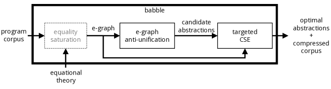
Figure 2. babble architecture overview

babble. We have implemented LLMT in babble, a tool built on top of the egg e-graph library (Willsey et al., 2021). The overview of the babble’s workflow is shown in Fig. 2, with gray boxes representing existing techniques and black boxes representing our contributions.

We evaluated babble on benchmarks from two sources: compression tasks extracted from DreamCoder runs (Bowers, 2022) and 2d cad programs used to evaluate concept learning in humans (Wong et al., 2022). Our evaluation shows that babble outperforms DreamCoder on its own benchmarks, achieving better compression in orders of magnitude less time. Adding domain-specific rewrites improves compression even further. We also show that babble scales to the larger 2d cad corpora, which is beyond reach of DreamCoder. We also present and discuss a selection of abstractions learned by babble, demonstrating that the LLMT approach can learn functions that match human intuition.

Contributions. In summary, this paper makes the following contributions:

• library learning modulo equational theory: a library learning algorithm that can incorporate an arbitrary domain-specific equational theory to make learning robust to syntactic variations;

• e-graph anti-unification: an algorithm that efficiently generates the set of candidate abstractions using the mechanism of anti-unification extended from terms to e-graphs;

• targeted common subexpression elimination: a new approximate algorithm for extracting the best term from an e-graph in the presence of common sub-expressions.

2. Overview

We illustrate LLMT via a running example building on Fig. 1. The input corpus in Fig. 1 is written in a 2d cad DSL by Wong et al. (2022), which features the following primitives:

line	a line segment from the origin (0, 0) to the point (1, 0)
${\mbox{\leavevmode\lstinline{{\lst@@@set@language\lst@@@set@numbers\lst@@@set@frame\lst@@@set@rulecolor\lst@@@set@language\small{\@listingGroup{ltx_lst_identifier}{combine}}}}}}(F_{1},\ F_{2})$	the union of figures $F_{1}$ and $F_{2}$
${\mbox{\leavevmode\lstinline{{\lst@@@set@language\lst@@@set@numbers\lst@@@set@frame\lst@@@set@rulecolor\lst@@@set@language\small{\@listingGroup{ltx_lst_identifier}{xform}}}}}}(F,\ \tau)$	applying transformation $\tau$ to figure $F$
${\mbox{\leavevmode\lstinline{{\lst@@@set@language\lst@@@set@numbers\lst@@@set@frame\lst@@@set@rulecolor\lst@@@set@language\small{\@listingGroup{ltx_lst_identifier}{repeat}}}}}}(F,\ 0,\ \tau)$	the empty figure
${\mbox{\leavevmode\lstinline{{\lst@@@set@language\lst@@@set@numbers\lst@@@set@frame\lst@@@set@rulecolor\lst@@@set@language\small{\@listingGroup{ltx_lst_identifier}{repeat}}}}}}(F,\ n+1,\ \tau)$	${{{\mbox{\leavevmode\lstinline{{\lst@@@set@language\lst@@@set@numbers\lst@@@set@frame\lst@@@set@rulecolor\lst@@@set@language\small{\@listingGroup{ltx_lst_identifier}{combine}}}}}}(F,\ \mbox{\leavevmode\lstinline{{\lst@@@set@language\lst@@@set@numbers\lst@@@set@frame\lst@@@set@rulecolor\lst@@@set@language\small{\@listingGroup{ltx_lst_identifier}{xform}}}}}}(\mbox{\leavevmode\lstinline{{\lst@@@set@language\lst@@@set@numbers\lst@@@set@frame\lst@@@set@rulecolor\lst@@@set@language\small{\@listingGroup{ltx_lst_identifier}{repeat}}}}}}(F,\ n,\ \tau),\ \tau))$, similar to a “fold”

A transformation $\tau$ is a 4-tuple $[s,\theta,t_{x},t_{y}]$ denoting uniformly scaling by a factor of $s$, rotating by $\theta$ radians, and translating by $(t_{x},\ t_{y})$ in the $x$ and $y$ directions respectively. For example, the green hexagon in Fig. 1 is implemented as:

$${{{{\mbox{\leavevmode\lstinline{{\lst@@@set@language\lst@@@set@numbers\lst@@@set@frame\lst@@@set@rulecolor\lst@@@set@language\small{\@listingGroup{ltx_lst_identifier}{xform}}}}}}(\mbox{\leavevmode\lstinline{{\lst@@@set@language\lst@@@set@numbers\lst@@@set@frame\lst@@@set@rulecolor\lst@@@set@language\small{\@listingGroup{ltx_lst_identifier}{repeat}}}}}}(\mbox{\leavevmode\lstinline{{\lst@@@set@language\lst@@@set@numbers\lst@@@set@frame\lst@@@set@rulecolor\lst@@@set@language\small{\@listingGroup{ltx_lst_identifier}{xform}}}}}}(\mbox{\leavevmode\lstinline{{\lst@@@set@language\lst@@@set@numbers\lst@@@set@frame\lst@@@set@rulecolor\lst@@@set@language\small{\@listingGroup{ltx_lst_identifier}{line}}}}}},\ [1,0,-0.5,0.5/\tan(\pi/6)]),\ 6,\ [1,2\pi/6,0,0]),\ [2,0,0,0])$$

That is, a hexagon side ${{\mbox{\leavevmode\lstinline{{\lst@@@set@language\lst@@@set@numbers\lst@@@set@frame\lst@@@set@rulecolor\lst@@@set@language\small{\@listingGroup{ltx_lst_identifier}{xform}}}}}}(\mbox{\leavevmode\lstinline{{\lst@@@set@language\lst@@@set@numbers\lst@@@set@frame\lst@@@set@rulecolor\lst@@@set@language\small{\@listingGroup{ltx_lst_identifier}{line}}}}}},\ [1,0,-0.5,0.5/\tan(\pi/6)])$ is repeated six times, each time rotated by another $2\pi/6$ radians, and the resulting unit hexagon is scaled by $2$.

Taking a closer look at the two blue hexagons in Fig. 1, however, we notice something peculiar. The two occurrences of ${{\mbox{\leavevmode\lstinline{{\lst@@@set@language\lst@@@set@numbers\lst@@@set@frame\lst@@@set@rulecolor\lst@@@set@language\small{\@listingGroup{ltx_lst_identifier}{xform}}}}}}(\mbox{\leavevmode\lstinline{{\lst@@@set@language\lst@@@set@numbers\lst@@@set@frame\lst@@@set@rulecolor\lst@@@set@language\small{\@listingGroup{ltx_lst_identifier}{repeat}}}}}}\ldots,\ [1,0,0,0])$ in Fig. 1 are no-ops: they merely scale a figure $F$ by a factor of 1 and neither rotate nor translate it. These redundant transformations would likely not be there had the code been written by hand or decompiled from a lower-level representation (by a tool like Szalinski (Nandi et al., 2020)); and yet, they are crucial if we hope to learn the optimal abstraction $f_{0}$ with a purely syntactic technique.

Fig. 3 shows a simplified and “more natural” version of the corpus from Fig. 1, which eliminates these no-op transformations. As illustrated in the figure, this causes a purely syntactic technique to learn a different function, $f_{1}$, which abstracts over an unscaled unit polygon. Because the scaling transformation is now outside the abstraction, it must be repeated five times. As a result, although the simplified input corpus C from Fig. 3 is smaller than the original corpus A (196 AST nodes instead of 208), its compressed version D is larger (81 AST nodes instead of 72)! In other words, syntactic library learning is not robust with respect to semantics-preserving code variations.

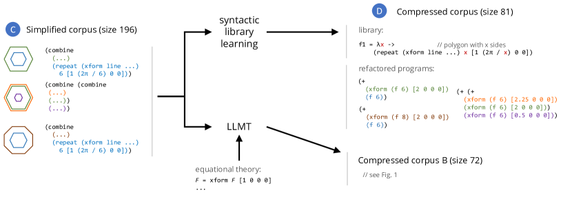
Figure 3. Difference between syntactic library learning and LLMT. Here the initial corpus C is the simplified version of corpus A from Fig. 1, with the redundant transformations on the blue subterms removed (unchanged terms are shown as ellipses). With this modification, syntactic techniques would learn an inferior abstraction $f_{1}$, leading to corpus D, while LLMT still learns the better abstraction $f_{0}$.

In contrast, our tool babble can take the simplified corpus C as input and still discover, in a fraction of a second, the scaled polygon abstraction $f_{0}$, yielding the compressed corpus B of size 72. In the rest of this section, we illustrate how babble achieves this using our new algorithm, library learning modulo equational theory (LLMT).

Simplified DSL. In the rest of this section we use a tailored version of the 2d cad DSL with the following additional constructs:

${\mbox{\leavevmode\lstinline{{\lst@@@set@language\lst@@@set@numbers\lst@@@set@frame\lst@@@set@rulecolor\lst@@@set@language\small{\@listingGroup{ltx_lst_identifier}{scale}}}}}}(F,\ s)$	scale $F$ by a factor of $s$
${\mbox{\leavevmode\lstinline{{\lst@@@set@language\lst@@@set@numbers\lst@@@set@frame\lst@@@set@rulecolor\lst@@@set@language\small{\@listingGroup{ltx_lst_identifier}{repRot}}}}}}(F,\ n,\ \theta)$	a special case of repeat that only performs rotation between iterations
${\mbox{\leavevmode\lstinline{{\lst@@@set@language\lst@@@set@numbers\lst@@@set@frame\lst@@@set@rulecolor\lst@@@set@language\small{\@listingGroup{ltx_lst_identifier}{side}}}}}}(n)$	a side of a regular unit $n$-gon

These are expressible in the original DSL, and could be even discovered with library learning, given an appropriate corpus; we treat them as primitives here for the sake of simplifying presentation.

2.1. Representing Equivalent Terms with E-Graphs

To exploit equivalences during library learning, babble takes as input a domain-specific equational theory. For our running example, let us assume that the theory contains a single equation:

(1) $${F\equiv\mbox{\leavevmode\lstinline{{\lst@@@set@language\lst@@@set@numbers\lst@@@set@frame\lst@@@set@rulecolor\lst@@@set@language\small{\@listingGroup{ltx_lst_identifier}{scale}}}}}}(F,\ 1)$$

which stipulates that any figure $F$ is equivalent to itself scaled by one. With this equation in hand, it is possible to “rewrite” corpus C into corpus A, and from there learn the optimal compressed corpus B by purely syntactic techniques. The challenge is that there are infinitely many alternative corpora C may be rewritten to; how do we know which to pick to maximize syntactic alignment, and thus the chance of discovering an optimal abstraction?

Instead of trying to guess the best equivalent corpus or enumerating them one by one, babble uses equality saturation (Tate et al., 2009; Willsey et al., 2021). Equality saturation takes as input a term $t$ and a set of rewrite rules, and finds the space of all terms equivalent to $t$ under the given rules; this is possible due to the high degree of sharing provided by the e-graph data structure, which can compactly represent the resulting space.

Fig. 4 (left) shows the e-graph built by equality saturation for the blue term in Fig. 3—represented in the simplified DSL as ${{\mbox{\leavevmode\lstinline{{\lst@@@set@language\lst@@@set@numbers\lst@@@set@frame\lst@@@set@rulecolor\lst@@@set@language\small{\@listingGroup{ltx_lst_identifier}{repRot}}}}}}(\mbox{\leavevmode\lstinline{{\lst@@@set@language\lst@@@set@numbers\lst@@@set@frame\lst@@@set@rulecolor\lst@@@set@language\small{\@listingGroup{ltx_lst_identifier}{side}}}}}}(6),\ 6,\ 2\pi/6)$—using the rewrite rule (1). The blue part of the graph represents the original term, and the gray part is added by equality saturation. The solid rectangles in the e-graph denote e-nodes (which are similar to regular AST nodes), while the dashed rectangles denote e-classes (which represent equivalence classes of terms). Importantly, the edges in the e-graph go from e-nodes to e-classes, which enables compact representation of programs with variation in sub-terms: for example, making e-class $c_{1}$ the first child of the repRot node, enables it to represent both terms ${{\mbox{\leavevmode\lstinline{{\lst@@@set@language\lst@@@set@numbers\lst@@@set@frame\lst@@@set@rulecolor\lst@@@set@language\small{\@listingGroup{ltx_lst_identifier}{repRot}}}}}}(\mbox{\leavevmode\lstinline{{\lst@@@set@language\lst@@@set@numbers\lst@@@set@frame\lst@@@set@rulecolor\lst@@@set@language\small{\@listingGroup{ltx_lst_identifier}{side}}}}}}(6),\ 6,\ 2\pi/6)$ and ${{{\mbox{\leavevmode\lstinline{{\lst@@@set@language\lst@@@set@numbers\lst@@@set@frame\lst@@@set@rulecolor\lst@@@set@language\small{\@listingGroup{ltx_lst_identifier}{repRot}}}}}}(\mbox{\leavevmode\lstinline{{\lst@@@set@language\lst@@@set@numbers\lst@@@set@frame\lst@@@set@rulecolor\lst@@@set@language\small{\@listingGroup{ltx_lst_identifier}{scale}}}}}}(\mbox{\leavevmode\lstinline{{\lst@@@set@language\lst@@@set@numbers\lst@@@set@frame\lst@@@set@rulecolor\lst@@@set@language\small{\@listingGroup{ltx_lst_identifier}{side}}}}}}(6),\ 1),\ 6,\ 2\pi/6)$ without duplicating their common parts. Furthermore, because e-graphs can have cycles, they can also represent infinite sets of terms: for example, the e-class $c_{1}$ represents all terms of the form: ${\mbox{\leavevmode\lstinline{{\lst@@@set@language\lst@@@set@numbers\lst@@@set@frame\lst@@@set@rulecolor\lst@@@set@language\small{\@listingGroup{ltx_lst_identifier}{side}}}}}}(6)$, ${{\mbox{\leavevmode\lstinline{{\lst@@@set@language\lst@@@set@numbers\lst@@@set@frame\lst@@@set@rulecolor\lst@@@set@language\small{\@listingGroup{ltx_lst_identifier}{scale}}}}}}(\mbox{\leavevmode\lstinline{{\lst@@@set@language\lst@@@set@numbers\lst@@@set@frame\lst@@@set@rulecolor\lst@@@set@language\small{\@listingGroup{ltx_lst_identifier}{side}}}}}}(6),\ 1)$, ${{{\mbox{\leavevmode\lstinline{{\lst@@@set@language\lst@@@set@numbers\lst@@@set@frame\lst@@@set@rulecolor\lst@@@set@language\small{\@listingGroup{ltx_lst_identifier}{scale}}}}}}(\mbox{\leavevmode\lstinline{{\lst@@@set@language\lst@@@set@numbers\lst@@@set@frame\lst@@@set@rulecolor\lst@@@set@language\small{\@listingGroup{ltx_lst_identifier}{scale}}}}}}(\mbox{\leavevmode\lstinline{{\lst@@@set@language\lst@@@set@numbers\lst@@@set@frame\lst@@@set@rulecolor\lst@@@set@language\small{\@listingGroup{ltx_lst_identifier}{side}}}}}}(6),\ 1),\ 1)$, etc. Because this e-graph represents the space of all equivalent terms up to the rewrite (1), the term we seek for library learning, namely ${{{\mbox{\leavevmode\lstinline{{\lst@@@set@language\lst@@@set@numbers\lst@@@set@frame\lst@@@set@rulecolor\lst@@@set@language\small{\@listingGroup{ltx_lst_identifier}{scale}}}}}}(\mbox{\leavevmode\lstinline{{\lst@@@set@language\lst@@@set@numbers\lst@@@set@frame\lst@@@set@rulecolor\lst@@@set@language\small{\@listingGroup{ltx_lst_identifier}{repRot}}}}}}(\mbox{\leavevmode\lstinline{{\lst@@@set@language\lst@@@set@numbers\lst@@@set@frame\lst@@@set@rulecolor\lst@@@set@language\small{\@listingGroup{ltx_lst_identifier}{side}}}}}}(6),\ 6,\ 2\pi/6),\ 1)$, is also represented in the e-class $c_{0}$.

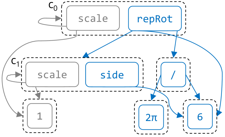
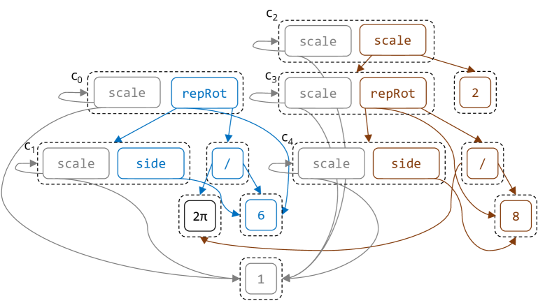
Figure 4. (Left) An e-graph representing the space of all programs equivalent the blue term in Fig. 3 under rule (1). (Right) An e-graph with both the blue and the brown terms from Fig. 3 after equality saturation. All terms are written in the simplified DSL.

2.2. Candidate Generation via E-Graph Anti-Unification

After building an e-graph from the given corpus by running equality saturation with the given equational theory, the next step in library learning is to generate candidate patterns that capture syntactic similarities across the corpus. The challenge is to generate sufficiently few candidates to make library learning tractable, but sufficiently many to achieve good compression. We illustrate candidate generation using the e-graph in Fig. 4 (right), which represents the part of our corpus consisting of the (saturated) blue and brown terms. Recall that the optimal pattern—which corresponds to the scaled polygon abstraction $f_{0}$—is:

(2) $${{{P_{0}=\mbox{\leavevmode\lstinline{{\lst@@@set@language\lst@@@set@numbers\lst@@@set@frame\lst@@@set@rulecolor\lst@@@set@language\small{\@listingGroup{ltx_lst_identifier}{scale}}}}}}(\mbox{\leavevmode\lstinline{{\lst@@@set@language\lst@@@set@numbers\lst@@@set@frame\lst@@@set@rulecolor\lst@@@set@language\small{\@listingGroup{ltx_lst_identifier}{repRot}}}}}}(\mbox{\leavevmode\lstinline{{\lst@@@set@language\lst@@@set@numbers\lst@@@set@frame\lst@@@set@rulecolor\lst@@@set@language\small{\@listingGroup{ltx_lst_identifier}{side}}}}}}(X),\ X,\ 2\pi/X),\ Y)$$

Prior work on DreamCoder generates patterns by picking a random fragment from the corpus, and then replacing arbitrarily chosen subterms with pattern variables. For example, to generate the pattern $P_{0}$, DreamCoder needs to pick the entire brown subterm as a fragment, and then decide to abstract over its subterms $8$ and $2$. This approach successfully restricts the set of candidates from all syntactically valid patterns to only those that have at least one match in the corpus; however, since there are too many ways to select the subterms to abstract over, this space is still too large to explore exhaustively beyond small corpora of short programs. In babble, this problem is exacerbated by equality saturation, since the e-graph often contains exponentially or infinitely more programs than the original corpus.

Generality Filters. To further prune the set of viable candidates in babble, we identify two classes of patterns that can be safely discarded, either because they are too concrete or too abstract. First, a pattern like ${{\mbox{\leavevmode\lstinline{{\lst@@@set@language\lst@@@set@numbers\lst@@@set@frame\lst@@@set@rulecolor\lst@@@set@language\small{\@listingGroup{ltx_lst_identifier}{repRot}}}}}}(\mbox{\leavevmode\lstinline{{\lst@@@set@language\lst@@@set@numbers\lst@@@set@frame\lst@@@set@rulecolor\lst@@@set@language\small{\@listingGroup{ltx_lst_identifier}{side}}}}}}(8),\ X,\ 2\pi/8)$ can be discarded because it is too concrete for this corpus: the corresponding abstraction can be applied only once, essentially replacing the sole matching term, ${{\mbox{\leavevmode\lstinline{{\lst@@@set@language\lst@@@set@numbers\lst@@@set@frame\lst@@@set@rulecolor\lst@@@set@language\small{\@listingGroup{ltx_lst_identifier}{repRot}}}}}}(\mbox{\leavevmode\lstinline{{\lst@@@set@language\lst@@@set@numbers\lst@@@set@frame\lst@@@set@rulecolor\lst@@@set@language\small{\@listingGroup{ltx_lst_identifier}{side}}}}}}(8),\ 8,\ 2\pi/8)$ with ${{(\lambda x\ \mathbf{\shortrightarrow}\ \mbox{\leavevmode\lstinline{{\lst@@@set@language\lst@@@set@numbers\lst@@@set@frame\lst@@@set@rulecolor\lst@@@set@language\small{\@listingGroup{ltx_lst_identifier}{repeat}}}}}}(\mbox{\leavevmode\lstinline{{\lst@@@set@language\lst@@@set@numbers\lst@@@set@frame\lst@@@set@rulecolor\lst@@@set@language\small{\@listingGroup{ltx_lst_identifier}{side}}}}}}(8),\ x,\ 2\pi/8))\ 8$, which only adds more AST nodes to the corpus. Second, a pattern like ${{\mbox{\leavevmode\lstinline{{\lst@@@set@language\lst@@@set@numbers\lst@@@set@frame\lst@@@set@rulecolor\lst@@@set@language\small{\@listingGroup{ltx_lst_identifier}{repRot}}}}}}(\mbox{\leavevmode\lstinline{{\lst@@@set@language\lst@@@set@numbers\lst@@@set@frame\lst@@@set@rulecolor\lst@@@set@language\small{\@listingGroup{ltx_lst_identifier}{side}}}}}}(X),\ X,\ Y)$ can be discarded because it is too abstract for this corpus: everywhere it matches, a more concrete pattern ${{\mbox{\leavevmode\lstinline{{\lst@@@set@language\lst@@@set@numbers\lst@@@set@frame\lst@@@set@rulecolor\lst@@@set@language\small{\@listingGroup{ltx_lst_identifier}{repRot}}}}}}(\mbox{\leavevmode\lstinline{{\lst@@@set@language\lst@@@set@numbers\lst@@@set@frame\lst@@@set@rulecolor\lst@@@set@language\small{\@listingGroup{ltx_lst_identifier}{side}}}}}}(X),\ X,\ 2\pi/X)$ would also match; using the more concrete pattern leads to better compression, since the actual arguments in its applications are both fewer and smaller: f 6 2$\pi$/6 and f 8 2$\pi$/8 vs. f 6 and f 8.

Thus, our first key insight is to restrict the set of candidates to the most concrete patterns that match some pair of subterms in the (saturated) corpus. For example, pattern $P_{0}$ is the most concrete pattern that matches the two terms

(3) $${{{\displaystyle\mbox{\leavevmode\lstinline{{\lst@@@set@language\lst@@@set@numbers\lst@@@set@frame\lst@@@set@rulecolor\lst@@@set@language\small{\@listingGroup{ltx_lst_identifier}{scale}}}}}}(\mbox{\leavevmode\lstinline{{\lst@@@set@language\lst@@@set@numbers\lst@@@set@frame\lst@@@set@rulecolor\lst@@@set@language\small{\@listingGroup{ltx_lst_identifier}{repRot}}}}}}(\mbox{\leavevmode\lstinline{{\lst@@@set@language\lst@@@set@numbers\lst@@@set@frame\lst@@@set@rulecolor\lst@@@set@language\small{\@listingGroup{ltx_lst_identifier}{side}}}}}}(6),\ 6,\ 2\pi/6),\ 1)$$

(4) $${{{\displaystyle\mbox{\leavevmode\lstinline{{\lst@@@set@language\lst@@@set@numbers\lst@@@set@frame\lst@@@set@rulecolor\lst@@@set@language\small{\@listingGroup{ltx_lst_identifier}{scale}}}}}}(\mbox{\leavevmode\lstinline{{\lst@@@set@language\lst@@@set@numbers\lst@@@set@frame\lst@@@set@rulecolor\lst@@@set@language\small{\@listingGroup{ltx_lst_identifier}{repRot}}}}}}(\mbox{\leavevmode\lstinline{{\lst@@@set@language\lst@@@set@numbers\lst@@@set@frame\lst@@@set@rulecolor\lst@@@set@language\small{\@listingGroup{ltx_lst_identifier}{side}}}}}}(8),\ 8,\ 2\pi/8),\ 2)$$

represented in Fig. 4 by the e-classes $c_{0}$ and $c_{2}$, respectively.

Term Anti-Unification. Computing the most concrete pattern that matches two given terms is known as anti-unification (AU) (Reynolds, 1969; Plotkin, 1970). AU works by a simple top-down traversal of the two terms, replacing any mismatched constructors by pattern variables. For example, to anti-unify the terms (3) and (4), we start from the root of both terms; since both AST nodes share the same constructor scale, it becomes part of the pattern and we recurse into the children. We eventually encounter a mismatch, where the term on the left is 6 and the term on the right is 8; so we create a fresh pattern variable $X$ and remember the anti-substitution ${{\sigma=\{(\mbox{\leavevmode\lstinline{{\lst@@@set@language\lst@@@set@numbers\lst@@@set@frame\lst@@@set@rulecolor\lst@@@set@language\small 6}}}},\mbox{\leavevmode\lstinline{{\lst@@@set@language\lst@@@set@numbers\lst@@@set@frame\lst@@@set@rulecolor\lst@@@set@language\small 8}}}})\mapsto X\}$. When we encounter a mismatch in the denominator of the angle, we look up the pair of mismatched terms ${{(\mbox{\leavevmode\lstinline{{\lst@@@set@language\lst@@@set@numbers\lst@@@set@frame\lst@@@set@rulecolor\lst@@@set@language\small 6}}}},\mbox{\leavevmode\lstinline{{\lst@@@set@language\lst@@@set@numbers\lst@@@set@frame\lst@@@set@rulecolor\lst@@@set@language\small 8}}}})$ in $\sigma$; because we already created a variable for this pair, we simply return the existing variable $X$. The final mismatch is ${{(\mbox{\leavevmode\lstinline{{\lst@@@set@language\lst@@@set@numbers\lst@@@set@frame\lst@@@set@rulecolor\lst@@@set@language\small 1}}}},\mbox{\leavevmode\lstinline{{\lst@@@set@language\lst@@@set@numbers\lst@@@set@frame\lst@@@set@rulecolor\lst@@@set@language\small 2}}}})$ in the second child of scale; since this pair is not yet in $\sigma$, we create a second pattern variable, $Y$. At this point, the resulting anti-unifier is the pattern $P_{0}$ (2).

Anti-unifying a single pair of terms is simple and efficient. However, in LLMT we want to anti-unify all pairs of subterms that can occur in any corpus equivalent (modulo the given equational theory) to the original. Explicitly enumerating all equivalent corpora represented by the e-graph and then performing AU on each pair of subterms is infeasible. Instead, babble performs anti-unification directly on the e-graph.

From Terms to E-Classes. We first explain how to anti-unify two e-classes. This operation takes as input a pair of e-classes and returns a set of dominant anti-unifiers, i.e. a set of patterns that (1) match both e-classes, and (2) is guaranteed to include the best abstraction among the most concrete patterns that match pairs of terms represented by the two e-classes.

Consider computing $\mathsf{AU}(c_{1},c_{4})$ for the e-classes $c_{1}$ and $c_{4}$ in the e-graph from Fig. 4 (right). AU still proceeds as a top-down traversal, but in this context we must check whether two e-classes have any constructors in common. In this case they do: both a side constructor and a scale constructor. Let us first pick the two side constructors and recurse into their only child, computing ${{\mathsf{AU}(\{\mbox{\leavevmode\lstinline{{\lst@@@set@language\lst@@@set@numbers\lst@@@set@frame\lst@@@set@rulecolor\lst@@@set@language\small 6}}}}\},\{\mbox{\leavevmode\lstinline{{\lst@@@set@language\lst@@@set@numbers\lst@@@set@frame\lst@@@set@rulecolor\lst@@@set@language\small 8}}}}\})$. These two e-classes have no matching constructors, so AU simply returns a pattern variable, similarly to term anti-unification; this yields the first pattern for $c_{1}$ and $c_{4}$: ${\mbox{\leavevmode\lstinline{{\lst@@@set@language\lst@@@set@numbers\lst@@@set@frame\lst@@@set@rulecolor\lst@@@set@language\small{\@listingGroup{ltx_lst_identifier}{side}}}}}}\ X$.

Recall, however, that $c_{1}$ and $c_{4}$ also have matching scale constructors. This is where things get interesting: these constructors are involved in a cycle (their first child is the parent e-class itself). If we let AU follow this cycle, the set of anti-unifiers becomes infinite:

$${{\mathsf{AU}(c_{1},c_{4})=\{\mbox{\leavevmode\lstinline{{\lst@@@set@language\lst@@@set@numbers\lst@@@set@frame\lst@@@set@rulecolor\lst@@@set@language\small{\@listingGroup{ltx_lst_identifier}{side}}}}}}\ X\}\cup\{\mbox{\leavevmode\lstinline{{\lst@@@set@language\lst@@@set@numbers\lst@@@set@frame\lst@@@set@rulecolor\lst@@@set@language\small{\@listingGroup{ltx_lst_identifier}{scale}}}}}}\ p\ 1\mid p\in\mathsf{AU}(c_{1},c_{4})\}$$

Fortunately, we can show that ${\mbox{\leavevmode\lstinline{{\lst@@@set@language\lst@@@set@numbers\lst@@@set@frame\lst@@@set@rulecolor\lst@@@set@language\small{\@listingGroup{ltx_lst_identifier}{side}}}}}}\ X$ dominates all the other patterns from this set, because their pattern variables—in this case, just $X$—match the same e-classes, but they are also larger (in Sec. 4 we show how this domination relation lets us prune other patterns, not just those caused by cycles). Hence $\mathsf{AU}(c_{1},c_{4})$ simply returns ${\{\mbox{\leavevmode\lstinline{{\lst@@@set@language\lst@@@set@numbers\lst@@@set@frame\lst@@@set@rulecolor\lst@@@set@language\small{\@listingGroup{ltx_lst_identifier}{side}}}}}}\ X\}$.

Following the same logic for the root e-classes of the two polygons, $c_{0}$ and $c_{2}$, $\mathsf{AU}(c_{0},c_{2})$ yields that pattern $P_{0}$ (2), which is required to learn the optimal abstraction.

From E-Classes to E-Graphs. To obtain the set of all candidate abstractions, we need to perform anti-unification over all pairs of e-classes in the e-graph. Clearly, these computations have overlapping subproblems (for example, we have to compute $\mathsf{AU}(c_{1},c_{4})$ as part of $\mathsf{AU}(c_{0},c_{2})$ and $\mathsf{AU}(c_{0},c_{3})$). To avoid duplicating work, babble uses an efficient dynamic programming algorithm that processes all pairs of e-classes in a bottom-up fashion.

2.3. Candidate Selection via Targeted Common Subexpression Elimination

We now illustrate the final step of library learning in babble: given the set of candidate abstractions generated by e-graph anti-unification, the goal is to pick a subset that gives the best compression for the corpus as a whole. For example, the candidates generated for the corpus from Fig. 3 include:

$${{{{{{{{\begin{array}[]{rcll}f_{0}&=&\lambda x\ y\ \mathbf{\shortrightarrow}\ \mbox{\leavevmode\lstinline{{\lst@@@set@language\lst@@@set@numbers\lst@@@set@frame\lst@@@set@rulecolor\lst@@@set@language\small{\@listingGroup{ltx_lst_identifier}{scale}}}}}}(\mbox{\leavevmode\lstinline{{\lst@@@set@language\lst@@@set@numbers\lst@@@set@frame\lst@@@set@rulecolor\lst@@@set@language\small{\@listingGroup{ltx_lst_identifier}{repRot}}}}}}(\mbox{\leavevmode\lstinline{{\lst@@@set@language\lst@@@set@numbers\lst@@@set@frame\lst@@@set@rulecolor\lst@@@set@language\small{\@listingGroup{ltx_lst_identifier}{side}}}}}}(x),\ x,\ 2\pi/x),\ y)&\quad\text{scaled regular $x$-gon}\\[2.0pt] f_{1}&=&\lambda x\ \mathbf{\shortrightarrow}\ \mbox{\leavevmode\lstinline{{\lst@@@set@language\lst@@@set@numbers\lst@@@set@frame\lst@@@set@rulecolor\lst@@@set@language\small{\@listingGroup{ltx_lst_identifier}{repRot}}}}}}(\mbox{\leavevmode\lstinline{{\lst@@@set@language\lst@@@set@numbers\lst@@@set@frame\lst@@@set@rulecolor\lst@@@set@language\small{\@listingGroup{ltx_lst_identifier}{side}}}}}}(x),\ x,\ 2\pi/x)&\quad\text{regular $x$-gon}\\[2.0pt] f_{2}&=&\lambda y\ \mathbf{\shortrightarrow}\ \mbox{\leavevmode\lstinline{{\lst@@@set@language\lst@@@set@numbers\lst@@@set@frame\lst@@@set@rulecolor\lst@@@set@language\small{\@listingGroup{ltx_lst_identifier}{scale}}}}}}(\mbox{\leavevmode\lstinline{{\lst@@@set@language\lst@@@set@numbers\lst@@@set@frame\lst@@@set@rulecolor\lst@@@set@language\small{\@listingGroup{ltx_lst_identifier}{repRot}}}}}}(\mbox{\leavevmode\lstinline{{\lst@@@set@language\lst@@@set@numbers\lst@@@set@frame\lst@@@set@rulecolor\lst@@@set@language\small{\@listingGroup{ltx_lst_identifier}{side}}}}}}(6),\ 6,\ 2\pi/6),\ y)&\quad\text{scaled hexagon}\end{array}$$

It is not immediately clear which abstraction is better: $f_{0}$ matches more terms than $f_{2}$, but $f_{2}$ requires fewer arguments (so if we have enough scaled hexagons in the corpus and only one octagon, it might be better to leave the octagon un-abstracted). On the other hand, $f_{1}$ might be better, since it does not introduce the redundant transformation on the blue hexagons. Finally, if we pick $f_{0}$ and $f_{2}$ together, we can also abstract the definition of $f_{2}$ as $f_{0}\ 6$, thereby getting additional reuse! As you can see, candidate selection is highly non-trivial, since it needs to take into account the choice between different equivalent programs in the e-graph, and the fact that some abstractions can be defined using others.

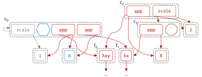
Figure 5. The e-graph from Fig. 4 (right) with applications of $f_{0}$ and $f_{1}$ depicted in red. We show the unchanged parts of the graph representing the unit hexagon and octagon as corresponding shapes; we also omit some of the gray e-nodes added in the previous stage.

Reduction to E-Graph Extraction. To overcome this difficulty, we once again leverage e-graph and equality saturation. Our second key insight is that selecting the optimal subset of abstractions can be reduced to the problem of extracting the smallest term from an e-graph in the presence of common sub-expressions.

To illustrate this reduction, let us limit our attention to only two candidate abstractions, $f_{0}$ and $f_{1}$, defined above. babble converts each of the candidate patterns and its corresponding abstraction into a rewrite rule that introduces a local $\lambda$-abstraction followed by application into the corpus; for our two abstractions these rules are:

(5) $${{{\displaystyle\mbox{\leavevmode\lstinline{{\lst@@@set@language\lst@@@set@numbers\lst@@@set@frame\lst@@@set@rulecolor\lst@@@set@language\small{\@listingGroup{ltx_lst_identifier}{scale}}}}}}(\mbox{\leavevmode\lstinline{{\lst@@@set@language\lst@@@set@numbers\lst@@@set@frame\lst@@@set@rulecolor\lst@@@set@language\small{\@listingGroup{ltx_lst_identifier}{repRot}}}}}}(\mbox{\leavevmode\lstinline{{\lst@@@set@language\lst@@@set@numbers\lst@@@set@frame\lst@@@set@rulecolor\lst@@@set@language\small{\@listingGroup{ltx_lst_identifier}{side}}}}}}(X),\ X,\ 2\pi/X),\ Y) \Rightarrow f_{0}\ X\ Y$$

(6) $${{\displaystyle\mbox{\leavevmode\lstinline{{\lst@@@set@language\lst@@@set@numbers\lst@@@set@frame\lst@@@set@rulecolor\lst@@@set@language\small{\@listingGroup{ltx_lst_identifier}{repRot}}}}}}(\mbox{\leavevmode\lstinline{{\lst@@@set@language\lst@@@set@numbers\lst@@@set@frame\lst@@@set@rulecolor\lst@@@set@language\small{\@listingGroup{ltx_lst_identifier}{side}}}}}}(X),\ X,\ 2\pi/X) \Rightarrow f_{1}\ X$$

The result of applying these rules to the e-graph from Fig. 4 (right) is shown in Fig. 5. For example, you can see that the e-class $c_{2}$ (which represents the scale-2 octagon) now stores an alternative representation: $f_{0}\ 8\ 2$. The e-class $c_{0}$ (unit hexagon) has representations using either $f_{0}$ or $f_{1}$, because this class matches both rewrite rules (5) and (6) above. Note also that because the definitions of the $\lambda$-abstractions are also stored in the e-graph, equality saturation can use the above rewrite rules inside their bodies, to make one function use another: for example, one term stored for the definition of $f_{0}$ is

$${\lambda x\ y\ \mathbf{\shortrightarrow}\ \mbox{\leavevmode\lstinline{{\lst@@@set@language\lst@@@set@numbers\lst@@@set@frame\lst@@@set@rulecolor\lst@@@set@language\small{\@listingGroup{ltx_lst_identifier}{scale}}}}}}(f_{1}\ x,\ y).$$

Once we have built the version of the e-graph with local lambdas for all the candidate abstractions, all that is left is to extract the smallest term out of this e-graph. The tricky part is that we want to count the size of the duplicated lambdas only once. For example, in Fig. 5, $f_{0}$ is applied twice (in $c_{0}$ and $c_{2}$); if term extraction were to choose both of these e-nodes, we want to treat their first child (the definition of $f_{0}$) as a common sub-expression, whose size contributes to the final expression only once. Intuitively, this is because we can “float” these lambdas into top-level let-bindings, thereby defining $f_{0}$ only once, and replacing each local lambda with a name.

Extraction with common sub-expressions is a known but notoriously hard problem, which is traditionally reduced to integer linear programming (ILP) (Yang et al., 2021; Wang et al., 2020). Because the scalability of the ILP approach is very limited, we have developed a custom extraction algorithm, which scales better by using domain-specific knowledge and approximation.

Extraction Algorithm. The main idea for making extraction more efficient is that for library learning we are only interested in sharing a certain type of sub-terms: namely, the $\lambda$-abstractions. Hence for each e-class we only need to keep track of the the best term for each possible library (i.e. each subset of $\lambda$-abstractions). More precisely, for each e-class and library, we keep track of (1) the smallest size of the library (2) the smallest size of the program refactored using this library (counting the $\lambda$-abstractions as a single node). We compute and propagate this information bottom-up through the e-graph. Once this information is computed for the root e-class (that represents the entire corpus), we can simply choose the library with the smallest total size.

For example, for the e-class $c_{2}$ from Fig. 5, with the empty library $\emptyset$, the size of library is 0 and the size of the smallest program (${{{\mbox{\leavevmode\lstinline{{\lst@@@set@language\lst@@@set@numbers\lst@@@set@frame\lst@@@set@rulecolor\lst@@@set@language\small{\@listingGroup{ltx_lst_identifier}{scale}}}}}}(\mbox{\leavevmode\lstinline{{\lst@@@set@language\lst@@@set@numbers\lst@@@set@frame\lst@@@set@rulecolor\lst@@@set@language\small{\@listingGroup{ltx_lst_identifier}{repRot}}}}}}(\mbox{\leavevmode\lstinline{{\lst@@@set@language\lst@@@set@numbers\lst@@@set@frame\lst@@@set@rulecolor\lst@@@set@language\small{\@listingGroup{ltx_lst_identifier}{side}}}}}}(8),\ 8,\ 2\pi/8),\ 2)$) is 9; with the library $\{f_{0}\}$, the size of the library is 9 and the size of the smallest program ($f_{0}\ 2\ 8$) is 3; while with the library $\{f_{1}\}$, the size of the library is 7 and the size of the smallest program (${\mbox{\leavevmode\lstinline{{\lst@@@set@language\lst@@@set@numbers\lst@@@set@frame\lst@@@set@rulecolor\lst@@@set@language\small{\@listingGroup{ltx_lst_identifier}{scale}}}}}}(f_{1}\ 8,\ 2)$) is 4. Clearly for this e-class introducing library functions is not paying off yet ($0+9<7+4<9+3$), since each one can be only used once. This situation changes, however, as we move up towards the root. Already for the parent e-class of $c_{0}$ and $c_{2}$, the cost of introducing $\{f_{0}\}$ and $\{f_{1}\}$ is amortized: the size of the smallest program is 17 with the empty library and 7 with either $\{f_{0}\}$ or $\{f_{1}\}$, so $\{f_{1}\}$ is already worthwhile to introduce ($9+7<0+17$). Including even more programs with scaled polygons eventually makes the library $\{f_{0}\}$ the most profitable of the four subsets.

Since in a larger corpus, keeping track of all subsets of candidate abstractions is not feasible, babble provides a way to trade off scalability and precision by using a beam search approach.

3. Library Learning over Terms

In this section we formalize the problem of library learning over a corpus of terms and motivate our first core contribution: generating candidate abstractions via anti-unification. Sec. 4 generalizes this formalism to library learning over an e-graph. For simplicity of exposition, our formalization of library learning is first order, that is, the initial corpus does not itself contain any $\lambda$-abstractions, and all the learned abstractions are first-order functions (the babble implementation does not have this limitation).

3.1. Preliminaries

Terms. A signature $\Sigma$ is a set of constructors, each associated with an arity. $\mathcal{T}(\Sigma)$ denotes the set of terms over $\Sigma$, defined as the smallest set containing all $s(t_{1},\dots,t_{k})$ where $s\in\Sigma$, $k=\mathsf{arity}(s)$, and $t_{1},\dots,t_{k}\in\mathcal{T}(\Sigma)$. We abbreviate nullary terms of the form $s()$ as $s$. The size of a term $\mathsf{size}(t)$ is defined in the usual way (as the number of constructors in the term). We use $\mathsf{subterms}(t)$ to denote the set of all subterms of $t$ (including $t$ itself). We assume that $\Sigma$ contains a dedicated variadic tuple constructor, written $\langle t_{1},\ldots,t_{n}\rangle$, which we use to represent a corpus of programs as a single term ($\langle\rangle$ does not contribute to the size of a term).

Patterns. If $\mathcal{X}$ is a denumerable set of variables, $\mathcal{T}(\Sigma,\mathcal{X})$ is a set of patterns, i.e. terms that can contain variables from $\mathcal{X}$. A pattern is linear if each of its variables occurs only once: $\forall X\in\mathsf{vars}(p).\mathsf{occurs}(X,p)=1$. A substitution $\sigma=[{X_{1}}\mapsto{p_{1}},\ldots,{X_{n}}\mapsto{p_{n}}]$ is a mapping from variables to patterns. We write ${\sigma}({p})$ to denote the application of $\sigma$ to pattern $p$, which is defined in the standard way. We define the size of a substitution $\mathsf{size}(\sigma)$ as the total size of its right-hand sides.

A pattern $p$ is more general than (or matches) $p^{\prime}$, written $p^{\prime}\sqsubseteq p$, if there exists $\sigma$ such that $p^{\prime}={\sigma}({p})$; we will denote such a $\sigma$ by $\mathsf{match}(p^{\prime},p)$. For example $X+1\sqsubseteq X+Y$ with $\mathsf{match}(X+1,X+Y)=[{Y}\mapsto{1}]$. The relation $\sqsubseteq$ is a partial order on patterns, and induces an equivalence relation $p_{1}\sim p_{2}\triangleq p_{1}\sqsubseteq p_{2}\wedge p_{2}\sqsubseteq p_{1}$ (equivalence up to variable renaming). In the following, we always distinguish patterns only up to this equivalence relation.

The join of two patterns $p_{1}\sqcup p_{2}$—also called their anti-unifier—is the least general pattern that matches both $p_{1}$ and $p_{2}$; the join is unique up to $\sim$. Note that $\langle\mathcal{T}(\Sigma,\mathcal{X}),\sqsubseteq,\sqcup,\top=X\rangle$ is a join semi-lattice (part of Plotkin’s subsumption lattice (Plotkin, 1970)). Consequently, the join can be generalized to an arbitrary set of patterns.

A context $\mathcal{C}$ is a pattern with a single occurrence of a distinguished variable $\circ$. We write $\mathcal{C}[p]$—$p$ in context $\mathcal{C}$—as a syntactic sugar for ${[{\circ}\mapsto{p}]}({\mathcal{C}})$. A rewrite rule $R$ is a pair of patterns, written $p_{1}\Rightarrow p_{2}$. Applying a rewrite rule $R$ to a term or pattern $p$, written ${R}({p})$ is defined in the standard way: ${R}({p})={(\mathsf{match}(p,p_{1}))}({p_{2}})$ if $p\sqsubseteq p_{1}$ and undefined otherwise. A pattern $p$ can be re-written in one step into $q$ using a rule $R$, written $p\rightarrow^{R}_{1}q$, if there exists a context $\mathcal{C}$ such that $p=\mathcal{C}[p^{\prime}]$ and $q=\mathcal{C}[{R}({p^{\prime}})]$. The reflexive-transitive closure of this relation is the rewrite relation $\rightarrow^{\mathcal{R}}$, where $\mathcal{R}$ is a set of rewrite rules.

Compressed Terms. Compressed terms $\hat{\mathcal{T}}(\Sigma,\mathcal{X})$ are of the form:

$$\hat{t}::=X\mid s(\hat{t}_{1},\ldots,\hat{t}_{k})\mid(\lambda X_{1}\ldots X_{n}\ \mathbf{\shortrightarrow}\ \hat{t})\ \hat{t}_{1}\ \ldots\ \hat{t}_{n}$$

In other words, compressed terms may contain applications of a $\lambda$-abstraction with zero or more binders to the same number of arguments. Note that this is a first-order language in the sense that all abstractions are fully applied. Importantly, we define $\mathsf{size}(\hat{t})$ in such a way that multiple occurrences of a $\lambda$-abstraction are only counted once. For simplicity of accounting, the size of an application $(\lambda\overline{X}\ \mathbf{\shortrightarrow}\ \hat{t}_{1})\ \overline{\hat{t}_{2}}$ is defined as $\mathsf{size}(\hat{t}_{1})+\sum{\overline{\mathsf{size}(\hat{t}_{2})}}$, that is, abstraction nodes themselves do not add to the size.

Beta-reduction on compressed terms, denoted $\hat{t}_{1}\rightarrow^{\beta}_{1}\hat{t}_{2}$, is defined in the usual way:

$$(\lambda\overline{X}\ \mathbf{\shortrightarrow}\ \hat{t}_{1})\ \overline{\hat{t}_{2}}\rightarrow^{\beta}_{1}{[\overline{X\mapsto\hat{t}_{2}}]}({\hat{t}_{1}})$$

where substitution on compressed terms is the standard capture-avoiding substitution for $\lambda$-calculus. Note that because our language is first-order and has no built-in recursion, it is strongly normalizing (the proof of this statement, as well as other proofs omitted from this section, can be found in the supplementary material). Hence, the order of $\beta$-reductions is irrelevant, and without loss of generality we can define evaluation on compressed terms, $\hat{t}_{1}\rightarrow^{\beta}\hat{t}_{2}$, to follow applicative order, i.e. innermost $\beta$-redexes are reduced first. As a result, any application reduced during evaluation has the form $(\lambda\overline{X}\ \mathbf{\shortrightarrow}\ p_{1})\ \overline{p_{2}}$, that is, neither the body $p_{1}$ nor the actual arguments $\overline{p_{2}}$ contain any redexes (and hence any $\lambda$-abstractions). This simplifies several aspects of our formalization; for example, there is no need for $\alpha$-renaming, since with no binders in $p_{1}$, no variable capture can occur.

Problem Statement. We can now formalize the library learning problem as follows: given a term $t\in\mathcal{T}(\Sigma)$, the goal is to find the smallest compressed term $\hat{t}\in\hat{\mathcal{T}}(\Sigma,\mathcal{X})$ that evaluates to $t$ (i.e. $\hat{t}\rightarrow^{\beta}t$). The reason such $\hat{t}$ may be smaller than $t$, is that it may contain multiple occurrences of the same $\lambda$-abstraction (applied to different arguments), whose size is only counted once. An example is shown in Fig. 6.

Although in full generality the solution might include nested lambdas with free variables (defined in the outer lambdas), in the rest of the paper we restrict our attention to global library learning, where all lambdas are closed terms. This is motivated by the purpose of library learning to discover reusable abstraction for a given problem domain. The solution in Fig. 6 already has this form.

$$\langle f(g(a)+g(a))+(g(1)+h(2))$$

$$,\ f(g(b)+g(b))+(g(3)+h(4))$$

$$,\ g(5)+h(6)\rangle$$

$$\langle\hat{f}_{2}\ g(a)\ 1\ 2,\hat{f}_{2}\ g(b)\ 2\ 3,\hat{f}_{1}\ 5\ 6\rangle\quad\text{where}$$

$$\hat{f}_{1}=\lambda Y\ Z\ \mathbf{\shortrightarrow}\ g(Y)+h(Z)$$

$$\hat{f}_{2}=\lambda X\ Y\ Z\ \mathbf{\shortrightarrow}\ f(X+X)+\hat{f}_{1}\ Y\ Z$$

Figure 6. Library learning. Left: initial term (size 29). Right: an optimal solution with two abstractions, one of which uses the other (size 26). A solution with $\hat{f}_{2}=\lambda X\ Y\ Z\ \mathbf{\shortrightarrow}\ f(g(X)+g(X))+\hat{f}_{1}\ Y\ Z$ also has size 26.

3.2. Pattern-Based Library Learning

At a high-level, our approach to library learning is to use patterns that occur in the original corpus as candidate bodies for $\lambda$-abstractions in the compressed corpus. Looking at the example in Fig. 6, it is not immediately obvious that using just the patterns from the original corpus is sufficient, since the body of $f_{2}$ contains an application of $f_{1}$. Perhaps surprisingly, this is not an issue: the key idea is that we can compress $t$ into $\hat{t}$ by inverting the evaluation $\hat{t}\rightarrow^{\beta}t$, and because the evaluation order is applicative, the rewritten sub-term at every step will not contain any $\beta$-redexes.

Compression. More formally, given a pattern $p$, let us define its compression rule (or $\kappa$-rule for short) as the rewrite rule

$$\kappa(p)\;\triangleq\;p\Rightarrow(\lambda\overline{X}\ \mathbf{\shortrightarrow}\ p)\ \overline{X}\quad\text{where}\quad\overline{X}=\mathsf{vars}(p)$$

In other words, $\kappa(p)$ will replace any term matching $p$ with an application of a function whose body is exactly $p$. For example, if $p=g(Y)+h(Z)$, its $\kappa$-rule is $g(Y)+h(Z)\Rightarrow(\lambda Y\ Z\ \mathbf{\shortrightarrow}\ g(Y)+h(Z))\ Y\ Z$. Note that on the right-hand side of this rule only the free occurrences of $Y$ and $Z$ will be substituted during rewriting; the bound $Y$ and $Z$ will be left unchanged, following the usual semantics of substitution for $\lambda$-calculus. For example, this rule can rewrite the third term in Fig. 6 (left) as follows:

$$g(5)+h(6)\;\rightarrow^{\kappa(g(Y)+h(Z))}_{1}\;(\lambda Y\ Z\ \mathbf{\shortrightarrow}\ g(Y)+h(Z))\ 5\ 6$$

A sequence of $\kappa$-rewrites $t\rightarrow^{\kappa(p_{1})}_{1}\dots\rightarrow^{\kappa(p_{n})}_{1}\hat{t}$, where all $p_{i}\in\mathcal{P}$, is called a compression of $t$ into $\hat{t}$ using patterns $\mathcal{P}$ and written $t\rightarrow^{\kappa(\mathcal{P})}\hat{t}$. We can now show that the library learning problem is equivalent to finding the smallest compression of $t$ using only patterns that occur in $t$.

Theorem 3.1 (Soundness and Completeness of Pattern-Based Library Learning).

For any term $t\in\mathcal{T}(\Sigma)$ and compressed term $\hat{t}\in\hat{\mathcal{T}}(\Sigma,\mathcal{X})$:

(Soundness):

If $t$ compresses into $\hat{t}$, then $\hat{t}$ evaluates to $t$: $\forall\mathcal{P}.t\rightarrow^{\kappa(\mathcal{P})}\hat{t}\Longrightarrow\hat{t}\rightarrow^{\beta}t$.

(Completeness):

If $\hat{t}$ is a solution to the (global) library learning problem, then $t$ compresses into $\hat{t}$ using only patterns that have a match in $t$: $\hat{t}\in\operatorname*{arg\,min}_{\hat{t}^{\prime}\rightarrow^{\beta}t}\mathsf{size}(\hat{t}^{\prime})\Longrightarrow t\rightarrow^{\kappa(\mathcal{P})}\hat{t}$, where $\mathcal{P}=\{p\in\mathcal{T}(\Sigma,\mathcal{X})\mid t^{\prime}\in\mathsf{subterms}(t),t^{\prime}\sqsubseteq p\}$.

The proof can be found in the supplementary material.

Example. Consider once again the library learning problem in Fig. 6. Here the set of patterns used to compress the original corpus into the solution on the right is:

$$p_{1}=g(Y)+h(Z)\quad\quad\quad p_{2}=f(X+X)+g(Y)+h(Z)$$

Rewriting the first term of the corpus proceeds in two steps (the redexes of $\kappa$-steps are highlighted):

$${\color[rgb]{0,0.21,0.79}f(g(a)+g(a))+(g(1)+h(2))}\;\rightarrow^{\kappa(p_{2})}_{1}\\ (\lambda X\ Y\ Z\ \mathbf{\shortrightarrow}\ f(X+X)+{\color[rgb]{0,0.21,0.79}g(Y)+h(Z)})\ g(a)\ g(a)\ (g(1)+h(2))\;\rightarrow^{\kappa(p_{1})}_{1}\\ (\lambda X\ Y\ Z\ \ \mathbf{\shortrightarrow}\ f(X+X)+(\lambda Y\ Z\ \mathbf{\shortrightarrow}\ g(Y)+h(Z))\ Y\ Z)\ g(a)\ g(a)\ (g(1)+h(2))$$

In other words, we first rewrite the entire term using $p_{2}$, and then rewrite inside the body of the introduced abstraction using $p_{1}$ (note that this order of compression is the inverse of the applicative evaluation order). The second term of the corpus compresses analogously; the third term compresses in a single step using $p_{1}$. Although this is not obvious from the rewrite sequence above, the resulting compressed corpus is indeed smaller than the original thanks to sharing of both $\lambda$-abstractions, as illustrated on the right of Fig. 6.

Library Learning as Term Rewriting. Theorem 3.1 reduces library learning to a term rewriting problem. Namely, given a term $t$ and a finite set of rewrite rules $\mathcal{R}=\{\kappa(p)\mid t^{\prime}\in\mathsf{subterms}(t),t^{\prime}\sqsubseteq p\}$, our goal is to find a minimal-size term $\hat{t}$ such that $t\rightarrow^{\mathcal{R}}\hat{t}$, which is a standard formulation in term rewriting. Unfortunately, this particular problem is notoriously difficult because (a) the rule set $\mathcal{R}$ is very large for any non-trivial term $t$, and (b) our $\mathsf{size}$ function is non-local (it takes sharing into account) In the rest of this section we discuss how we can prune the rule set $\mathcal{R}$ to reduce it to a tractable size. Sec. 5 discusses how we tackle the remaining term rewriting problem using the equality saturation technique (Tate et al., 2009; Willsey et al., 2021).

3.3. Pruning Candidate Patterns

In this section, we discuss which patterns can be discarded from consideration when constructing the set of $\kappa$-rules $\mathcal{R}$ for the term rewriting problem.

Cost of a Pattern. Consider a compression $t\rightarrow^{\kappa(\mathcal{P})}\hat{t}$ where each pattern $p\in\mathcal{P}$ is used some number $n$ times, with substitutions $\sigma^{p}_{1},\ldots,\sigma^{p}_{n}$. We can break down the total amount of compression into contributions of individual patterns:

$$\mathsf{size}(\hat{t})-\mathsf{size}(t)=\sum_{p\in\mathcal{P}}\mathsf{cost}(p,\{\sigma^{p}_{1},\dots\sigma^{p}_{n}\})$$

The cost of a pattern $p$, in turn, consists of three components. The cost of introducing the abstraction is the size of its body, i.e. $\mathsf{size}(p)$. The cost of using an abstraction—$\textsf{use}(p,\sigma)$ (7)—includes the application itself and the size of the arguments. The cost saved by using an abstraction—$\textsf{save}(p,\sigma)$ (8)—is just the cost of the term matched by $p$ (i.e. the redex of the corresponding $\kappa$-step).

(7) $$\textsf{use}(p,\sigma) =1+\sum_{X\in\mathsf{vars}(p)}\mathsf{size}(\sigma(X))$$

(8) $$\textsf{save}(p,\sigma) =\mathsf{size}({\sigma}({p}))=\mathsf{size}(p)+\sum_{X\in\mathsf{vars}(p)}\mathsf{occurs}(X,p)\cdot(\mathsf{size}(\sigma(X))-1)$$

The total cost of $p$ is the cost of introducing the abstraction paid a single time, plus the cost of each use, minus what you save for each application:

(9) $$\textsf{cost}(p,\{\sigma_{1},\ldots,\sigma_{n}\})=\mathsf{size}(p)+\sum_{\sigma_{i}}(\textsf{use}(p,\sigma_{i})-\textsf{save}(p,\sigma_{i}))$$

When $p$ is linear (all $\mathsf{occurs}(X,p)=1$), the cost depends only on $n$ but not on the substitutions $\sigma_{i}$:

(10) $$\textsf{cost}(p,\{\sigma_{1},\ldots,\sigma_{n}\}) =\mathsf{size}(p)+\sum_{\sigma_{i}}\left(1-\mathsf{size}(p)+|\mathsf{vars}(p)|\right)$$

(11) $$=\mathsf{size}(p)+n\cdot\left(1-\mathsf{size}(p)+|\mathsf{vars}(p)|\right)$$

We can show that a pattern $p$ with a non-negative cost can be safely discarded, that is: there exists another compression using only $\mathcal{P}\setminus\{p\}$, whose result is at least as small.

Trivial Patterns. Based on this analysis, any linear pattern $p$ with $\mathsf{skeleton}(p)\leq 1$ can be discarded, where $\mathsf{skeleton}(p)=\mathsf{size}(p)-|\mathsf{vars}(p)|$ is the size of $p$’s “skeleton”, i.e. it’s body without the variables. Intuitively, the skeleton of $p$ is simply too small to pay for introducing an application. In this case, $\mathsf{cost}(p,\_)>0$ independently of how many times it is used. We refer to such patterns as trivial. Examples of trivial patterns are $X$ and $X+Y$.

Patterns with a Single Match. We can show that patterns with only a single match in the corpus can also be discarded. If $p$ has a single match in $t$, then it can appear at most once in any compression of $t$. If $p$ is linear, $\mathsf{cost}(p,\_)=1+|\mathsf{vars}(p)|$, which is always positive, so $p$ can be discarded. But what about non-linear patterns, where even a single $\kappa$-step can decrease size thanks to variable reuse? It turns out that any non-linear pattern with a single match can always be replaced by a nullary pattern (with no variables) that is more optimal.

Without loss of generality, assume that $p$ has a single variable $X$ that occurs $m>1$ times, and let its sole $\kappa$-step be ${\sigma}({p})\rightarrow^{\kappa(p)}_{1}(\lambda X\ \mathbf{\shortrightarrow}\ p)\ {\sigma}({X})$. The size of the right-hand side is $\mathsf{size}(p)+1+\mathsf{size}({\sigma}({X}))$, or, rewritten in terms of $p$’s skeleton: $1+(\mathsf{skeleton}(p)+m)+\mathsf{size}({\sigma}({X}))$. Instead, we can rewrite the same redex ${\sigma}({p})\rightarrow^{\{R\}}p^{\prime}$ using $m$ applications of the rule $R\;\triangleq\;{\sigma}({X})\Rightarrow(\lambda\epsilon\ \mathbf{\shortrightarrow}\ {\sigma}({X}))\ \epsilon$. This is a $\kappa$-rule for a nullary pattern ${\sigma}({X})$ with no variables (hence the corresponding $\lambda$-abstraction has zero binders). The size of $p^{\prime}$ obtained in this way is $\mathsf{size}({\sigma}({X}))+m+\mathsf{skeleton}(p)$ (where the former is the size of the shared $\lambda$-abstraction, $m$ is the number of applications, and $\mathsf{skeleton}(p)$ is the size of the term around the applications). As you can see, this term is one smaller than the one we get by applying $p$. Intuitively, this result says that instead of using a non-linear pattern that occurs only once, it is better to perform common sub-expression elimination.

Parameterization Lattice. Eliminating from consideration all patterns with fewer than two matches in the corpus suggests an algorithm for generating a complete set $\mathcal{P}$ of candidate patterns: (1) start from the set $\mathcal{P}^{2}(t)=\{t_{1}\sqcup t_{2}\mid t_{i}\in\mathsf{subterms}(t)\}$ of all pairwise joins of subterms of the input program, (2) explore all elements of the subsumption semi-lattice above those patterns, by gradually replacing sub-patterns with variables, until we hit trivial patterns at the top of the lattice. We will refer to this semi-lattice above $\mathcal{P}^{2}(t)$ as the parametrization lattice of $t$, denoted $\mathcal{P}(t)$. A fragment of $\mathcal{P}(t)$ for $t=\langle f(a+b),f(a+c),f(b+c)\rangle$ is shown in Fig. 7 (left).

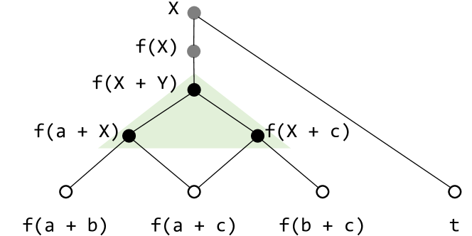
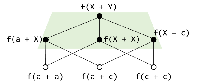
Figure 7. Left: fragment of the parametrization lattice for the term $t=\langle f(a+b),f(a+c),f(b+c)\rangle$; only filled black circles correspond to candidate patterns: hollow circles match fewer than two terms and gray circles are trivial. Right: an example where is it insufficient to consider pairwise joins to obtain an optimal pattern.

Approximation. In practice, computing the set $\mathcal{P}^{2}(t)$ is feasible: although there are quadratically many pairs of subterms, most of them do not have a common constructor at the root, and hence their join is trivially $X$. An example is the join of $t$ with any of its subterms in Fig. 7 (left). Unfortunately, generalizing the patterns from $\mathcal{P}^{2}(t)$ according to the parameterization lattice (Fig. 7) is expensive. For this reason, babble adopts an approximation and simply uses $\mathcal{P}^{2}(t)$ as the set of candidates.

This approximation makes our pattern generation theoretically incomplete. Consider a pattern $p\in\mathcal{P}(t)\setminus\mathcal{P}^{2}(t)$; there are two reasons why we might need $p$ in the optimal compression of $t$:

1. there is no $p^{\prime}\in\mathcal{P}^{2}(t)$ with the same set of matches as $p$, or

2. there is such a $p^{\prime}$ but it has few enough matches that its larger size does not pay off.

The first kind of incompleteness occurs when $p$ matches a set of subterms $t_{1},\ldots,t_{n}$ ($n>2$), whose join is distinct from all their pairwise joins (otherwise some $t_{i}\sqcup t_{j}\in\mathcal{P}^{2}(t)$ would also match all $t_{1},\ldots,t_{n}$). An example is shown in Fig. 7 (right), where the three subterms in question are $f(a+a)$, $f(a+c)$, and $f(c+c)$. In this case, an optimal compression might use the pattern $f(X+Y)$ to rewrite all three subterms, but our approximation would only include the patterns $f(a+X)$, $f(X+X)$, and $f(X+c)$, each of which can rewrite only two of the three subterms.

The second kind of incompleteness occurs when there exists $p^{\prime}\in\mathcal{P}^{2}(t)$ that has the same set of matches as $p$, despite being strictly more specific, and yet using $p^{\prime}$ instead of $p$ still doe not pay off. The understand when this happens, consider the difference in costs between $p$ and $p^{\prime}$, assuming that they are both used to rewrite the same $n$ subterms (i.e. their save cost is the same):

$$\mathsf{cost}(p^{\prime},\overline{\sigma^{\prime}})-\mathsf{cost}(p,\overline{\sigma}) =\mathsf{size}(p^{\prime})-\mathsf{size}(p)+\sum_{i}(\mathsf{use}(p^{\prime},\sigma^{\prime}_{i})-\mathsf{use}(p,\sigma_{i}))$$

$$=\mathsf{size}(p^{\prime})-\mathsf{size}(p)+\sum_{i}(\mathsf{size}(\sigma^{\prime}_{i})-\mathsf{size}(\sigma_{i}))$$

Because $p^{\prime}$ is strictly more specific than $p$, we know that $\mathsf{size}(p^{\prime})\geq\mathsf{size}(p)$, but all its substitutions $\sigma^{\prime}_{i}$ must be strictly smaller than $\sigma_{i}$. Hence, with enough uses, $p^{\prime}$ is bound to become more compressive than $p$; when there are just a few uses, however, $p$ can be more optimal. For example, consider the corpus $\langle\mathcal{C}[f(1,2,3)],\mathcal{C}[f(4,5,6)]\rangle$, where $\mathcal{C}$ is some sufficiently large context. Here, a more general pattern $p=\mathcal{C}[X]$ is more optimal than the more specific $p^{\prime}=\mathcal{C}[f(X,Y,Z)]$, because $\mathsf{size}(p^{\prime})-\mathsf{size}(p)=3$, each use of $p^{\prime}$ is only one node cheaper, and there are only two uses.

Despite the lack of theoretical completeness guarantees, we argue that restricting candidate patterns to $\mathcal{P}^{2}(t)$ is a reasonable trade-off. Note, that the counter-examples above are quite contrived, and they no longer apply once the corpus contains sufficiently many and sufficiently diverse instances of a pattern (for example, adding $f(b,b)$ to the first corpus would make $f(X,Y)$ appear in $\mathcal{P}^{2}(t)$, and adding just one more occurrence of $p^{\prime}$ into the second corpus would make it as optimal as $p$). Our empirical evaluation confirms that this approximation works well in practice.

4. Library Learning modulo Equational Theory

Syntax

$$\begin{array}[]{rll}\text{e-class ids}&a,b&\in\mathcal{I}\\ \text{e-nodes}&n\mathrel{\mathord{:}\mathord{:=}}s(a_{1},\ldots,a_{k})&\in N\\ \text{e-classes}&c\mathrel{\mathord{:}\mathord{:=}}\{n_{1},\ldots,n_{m}\}&\in C\end{array}$$

Denotation $\llbracket\cdot\rrbracket\colon N\to 2^{\mathcal{T}(\Sigma)}$, $\llbracket\cdot\rrbracket\colon C\to 2^{\mathcal{T}(\Sigma)}$

$$\begin{array}[]{rl}\\ \llbracket s(a_{1},\ldots,a_{k})\rrbracket&=\{s(t_{1},\ldots,t_{k})\mid t_{i}\in\llbracket M(a_{i})\rrbracket\}\\ \llbracket\{n_{1},\ldots,n_{m}\}\rrbracket&=\bigcup_{i\in[1,m]}\llbracket n_{i}\rrbracket\end{array}$$

Figure 8. Syntax, metavariables, and denotation for the components of an e-graph. Here $s\in\Sigma$ and $k=\mathsf{arity}(s)$.

E-Graphs. Let $\mathcal{I}$ be a denumerable set of e-class ids. An e-graph $\mathcal{G}$ is a triple $\langle C,M,r\rangle$, where $C$ is a set of e-classes, $M\colon\mathcal{I}\to C$ is an e-class map. and $r\in\mathcal{I}$ is the root class id. An e-class $c\in C$ is a set of e-nodes $n\in N$, and an e-node is a constructor applied to e-class ids. The syntax of e-classes and e-nodes is summarized in Fig. 8 (left). An e-graph has to satisfy the congruence invariant, which states that the e-graph has no two identical e-nodes (or alternatively, that all e-classes are disjoint).

The denotation of an e-graph—the set of terms it represents—is the denotation of its root e-class $\llbracket M(r)\rrbracket$, where the denotation of e-classes and e-nodes is defined mutually-recursively in Fig. 8 (right). Note that the denotation can be infinite if the e-graph has cycles. An e-graph induces an equivalence relation $\equiv^{\mathcal{G}}$, where $t_{1}\equiv^{\mathcal{G}}t_{2}$ iff there exists an e-class $c\in C$ such that $t_{1}\in\llbracket c\rrbracket\wedge t_{2}\in\llbracket c\rrbracket$.

E-graphs provide means to extract the cheapest term from an e-class according to some cost function: $\mathsf{extract}_{\mathsf{cost}}(a)=\operatorname*{arg\,min}_{t\in\llbracket M(a)\rrbracket}\mathsf{cost}(t)$. If $\mathsf{cost}$ is local, meaning that the cost of a term can be computed from the costs of its immediate children, extraction can be done efficiently by a greedy algorithm, which recursively extracts the best term from each e-class.

E-Matching. E-matching is a generalization of pattern matching to e-graphs, where matching an e-class $c$ against a pattern $p$ yields a set of e-class substitutions $\theta\colon\mathcal{X}\to\mathcal{I}$ such that ${\theta}({p})$ is a “subgraph” of $c$. To formalize this notion, we introduce partial terms $\pi\in\mathcal{T}(\Sigma,\mathcal{I})$, which are terms whose leaves can be e-class ids (or, alternatively, patterns with e-class ids for variables). The containment relation ${\pi}\prec{a}$ for some e-class id $a$ is defined as follows:

$${a}\prec{a}\quad\quad\quad{s(\pi_{1},\ldots,\pi_{k})}\prec{a}\ \text{iff}\ s(a_{1},\ldots,a_{k})\in M(a)\wedge{\pi_{i}}\prec{a_{i}}$$

With this definition, a pattern $p$ matches an e-class $a$, $a\sqsubseteq p$, if there exists an e-class substitution $\theta$, such that ${{\theta}({p})}\prec{a}$. We denote the set of such substitutions as $\mathsf{matches}(a,p)$.

Rewriting and Equality Saturation. Equality saturation (EqSat) (Tate et al., 2009; Willsey et al., 2021) takes as input a term $t$ and a set of equations that induce an equivalence relation $\equiv$, and produces an e-graph $\mathcal{G}$ such that $\llbracket\mathcal{G}\rrbracket=\{t^{\prime}\mid t\equiv t^{\prime}\}$ and $t\equiv t^{\prime}$ iff $t\equiv^{\mathcal{G}}t^{\prime}$. The core idea of EqSat is to convert equations into rewrite rules and apply them to the e-graph in a non-destructive way: so that the original term and the rewritten terms are both represented in the same e-class. Applying a rewrite rule $p_{1}\Rightarrow p_{2}$ to an e-class $a$ works as follows: for each $\theta\in\mathsf{matches}(a,p_{1})$, we obtain the rewritten partial term $\pi^{\prime}={\theta}({p_{2}})$ and then add this partial term to the same e-class $a$, restoring the congruence invariant (i.e. merging e-classes that now have identical e-nodes).

4.1. Top-Level Algorithm

⬇

1# Original term $t$, set of equational rewrite rules $\ruleset_\semeq$, maximum library size $N$

2def LLMT($t$, $R_\semeq$, $N$):

3 # EqSat phase:

4 $\mathcal{G}$ = egraph($t$) # initialize with a single term $t$

5 $\mathcal{G}$ = eqSat($\mathcal{G}, \ruleset_\semeq$) # $\mathcal{G}$ represents all terms that are $\semeq t$

6

7 # candidate generation phase:

8 $\patset$ = AU($\mathcal{G}$) # generate candidate patterns by anti-unification

9 $\ruleset_\kappa$ = $\{\kappa(p) \mid p \in \patset\}$ # construct a compression rule from every pattern

10 $\mathcal{G}’$ = eqSat($\mathcal{G}, \ruleset_\kappa$) # $\mathcal{G}’$ represents all ways to compress $\mathcal{G}$

11

12 # candidate selection phase:

13 $\ruleset’$ = select_library($\mathcal{G}’, N$) # select the best $N$ rules from $\ruleset_\kappa$ using beam search

14 $\mathcal{G}’’$ = eqSat($\mathcal{G}, R’$) # $\mathcal{G}’’$ represents all ways to compress $\mathcal{G}$ using the optimal library

15 return extract($\mathcal{G}’’$) # extract the smallest compressed term from $\mathcal{G}’’$’

Figure 9. The top-level LLMT algorithm.

We can formalize the problem of library learning modulo equational theory (LLMT) as follows: given a term $t$ and a set of equations that induce an equivalence relation $\equiv$, the goal is to find a compressed term $\hat{t}\in\hat{\mathcal{T}}(\Sigma,\mathcal{X})$, such that $\hat{t}\rightarrow^{\beta}t^{\prime}\equiv t$ (for some $t^{\prime}$), and $\hat{t}$ has a minimal size.

Our top-level algorithm LLMT is depicted in Fig. 9. This algorithm takes as input the original corpus $t$ and the equational theory, represented as a set of require rules $\mathcal{R}_{\equiv}$ (another input to the algorithm is the maximum size of the library; this parameter is introduced for the sake of efficiency, as we explain in Sec. 5). As the first step (lines 4–5), LLMT applies EqSat to obtain an e-graph $\mathcal{G}$ that represents all terms $t^{\prime}$ such that $t^{\prime}\equiv t$. This reduces the LLMT problem to library learning over an e-graph: i.e. the goal is to find a minimal-size compressed term $\hat{t}$, such that $\hat{t}\rightarrow^{\beta}t^{\prime}$ for some $t^{\prime}\in\llbracket\mathcal{G}\rrbracket$. Similarly to Sec. 3, we take a pattern-based approach to this problem, that is, we select a set $\mathcal{P}$ of candidate patterns and then perform compression rewrites using these patterns.

The rest of the algorithm is split into two phases: candidate generation and candidate selection. Candidate generation (lines 8–10) first computes the set of candidate patterns $\mathcal{P}$ using the anti-unification mechanism extended to e-graphs. Then it creates a compression rule ($\kappa$-rule, see Sec. 3) from each candidate pattern, and once again applies EqSat to obtain a new e-graph $\mathcal{G}^{\prime}$. This new e-graph represents all possible ways to compress the terms from $\mathcal{G}$ using patterns in $\mathcal{P}$. Finally, the candidate selection phase (lines 13–15) selects the optimal subset of compression rules $\mathcal{R}^{\prime}$, constructs an e-graph $\mathcal{G}^{\prime\prime}$ that represents all possible compressions using only the selected compression rules, and finally extracts the smallest compressed term from this e-graph.

The rest of this section focuses on the candidate generation via e-graph anti-unification (line 8). The candidate selection functions select_library and extract are discussed in Sec. 5.

4.2. Candidate Generation via E-Graph Anti-Unification

The goal of candidate generation is to find a set of patterns that are useful for compression. Following the discussion in Sec. 3, we restrict our attention to patterns $\mathsf{AU}(t_{1},t_{2})$, where $t_{1}$ and $t_{2}$ are subterms of some $t\in\llbracket\mathcal{G}\rrbracket$. The naïve approach is to enumerate all such $t$, and for each one, perform anti-unification on all pairs of subterms; this is suboptimal at best, and impossible at worst (when $\llbracket\mathcal{G}\rrbracket$ is infinite). Hence in this section we show how to compute a finite set of candidate patterns directly on the e-graph, without discarding any optimal patterns.

E-Class Anti-Unification. Let us first consider anti-unification of two e-classes, $\mathsf{AU}(a,b)$, which takes as input e-class ids $a$ and $b$ and returns a set of patterns. We define $\mathsf{AU}(a,b)=\mathsf{AU}(\epsilon\vdash a,b)$, where $\mathsf{AU}(\Gamma\vdash a,b)$ is an auxiliary function that additionally takes into account a context $\Gamma$. A context is a list of pairs of e-classes that have been visited while computing the AU, and is required to prevent infinite recursion in case of cycles in the e-graph.

E-node Anti-Unification $\mathsf{AU}(\Gamma\vdash n_{1},n_{2})$

$$\begin{array}[]{rl}\mathsf{AU}(\Gamma,(a,b)\vdash s(a_{1},\ldots,a_{k}),s(b_{1},\ldots,b_{k}))&=\{s(p_{1},\ldots,p_{k})\mid p_{i}\in\mathsf{AU}(\Gamma\vdash a_{i},b_{i})\}\\ \mathsf{AU}(\Gamma,(a,b)\vdash s_{1}(\ldots),s_{2}(\ldots))&=\{X_{a,b}\}\quad\text{if}\ s_{1}\neq s_{2}\\ \end{array}$$

E-class Anti-Unification $\mathsf{AU}(\Gamma\vdash a,b)$

$$\begin{array}[]{rl}\mathsf{AU}(\Gamma\vdash a,b)&=\emptyset\quad\text{if}\ (a,b)\in\Gamma\\ \mathsf{AU}(\Gamma\vdash a,b)&={\color[rgb]{0,0.21,0.79}\mathsf{dominant}}\left(\bigcup_{n_{a}\in M(a),n_{b}\in M(b)}\mathsf{AU}(\Gamma,(a,b)\vdash n_{a},n_{b})\right)\end{array}$$

Figure 10. E-class anti-unification defined as two mutually-recursive functions of e-nodes and e-class ids.

Fig. 10 defines this operation using two mutually recursive functions that anti-unify e-classes and e-nodes. Note that e-node AU is always invoked in a non-empty context. The first equation anti-unifies two e-nodes with the same constructor: in this case, we recursively anti-unify their child e-classes and return the cross-product of the results. The second equation applies to e-nodes with different constructors: as in term AU, this results in a pattern variable. A nice side-effect of dealing with e-graphs is that we need not keep track of the anti-substitution to guarantee that each pair of subterms maps to the same variable: because any duplicate terms are represented by the same e-class, we can simply use the e-class ids $a$ and $b$ in the name of the pattern variable $X_{a,b}$.

The second block of equations defines anti-unification of e-classes (let us first ignore the dominant which will be explained shortly). The first equation applies when $a$ and $b$ have already been visited: in this case, we break the cycle and return the empty set. Otherwise, the last equation anti-unifies all pairs of e-nodes from the two e-classes in an updated context and merges the results. Note that this will add a pattern variable unless all e-nodes in both e-classes have the same constructor; we have omitted this detail in Sec. 2 for simplicity, but this is implemented in babble and often yields more optimal patterns. For example, consider anti-unifying $c_{1}$ and $c_{2}$ from Fig. 4 (right): although they have the constructor scale in common, $X$ is actually a better pattern for abstracting these two e-classes than ${\mbox{\leavevmode\lstinline{{\lst@@@set@language\lst@@@set@numbers\lst@@@set@frame\lst@@@set@rulecolor\lst@@@set@language\small{\@listingGroup{ltx_lst_identifier}{scale}}}}}}\ X\ Y$, because the total size of the actual arguments to pattern $X$ (${\mbox{\leavevmode\lstinline{{\lst@@@set@language\lst@@@set@numbers\lst@@@set@frame\lst@@@set@rulecolor\lst@@@set@language\small{\@listingGroup{ltx_lst_identifier}{side}}}}}}(6)$ and ${{{\mbox{\leavevmode\lstinline{{\lst@@@set@language\lst@@@set@numbers\lst@@@set@frame\lst@@@set@rulecolor\lst@@@set@language\small{\@listingGroup{ltx_lst_identifier}{scale}}}}}}(\mbox{\leavevmode\lstinline{{\lst@@@set@language\lst@@@set@numbers\lst@@@set@frame\lst@@@set@rulecolor\lst@@@set@language\small{\@listingGroup{ltx_lst_identifier}{repRot}}}}}}(\mbox{\leavevmode\lstinline{{\lst@@@set@language\lst@@@set@numbers\lst@@@set@frame\lst@@@set@rulecolor\lst@@@set@language\small{\@listingGroup{ltx_lst_identifier}{side}}}}}}(8),\ 8,\ 2\pi/8),\ 2)$) is the same as those to the pattern ${\mbox{\leavevmode\lstinline{{\lst@@@set@language\lst@@@set@numbers\lst@@@set@frame\lst@@@set@rulecolor\lst@@@set@language\small{\@listingGroup{ltx_lst_identifier}{scale}}}}}}\ X\ Y$ (${\mbox{\leavevmode\lstinline{{\lst@@@set@language\lst@@@set@numbers\lst@@@set@frame\lst@@@set@rulecolor\lst@@@set@language\small{\@listingGroup{ltx_lst_identifier}{side}}}}}}(6)$, $1$, ${{\mbox{\leavevmode\lstinline{{\lst@@@set@language\lst@@@set@numbers\lst@@@set@frame\lst@@@set@rulecolor\lst@@@set@language\small{\@listingGroup{ltx_lst_identifier}{repRot}}}}}}(\mbox{\leavevmode\lstinline{{\lst@@@set@language\lst@@@set@numbers\lst@@@set@frame\lst@@@set@rulecolor\lst@@@set@language\small{\@listingGroup{ltx_lst_identifier}{side}}}}}}(8),\ 8,\ 2\pi/8)$, and $2$), and the pattern $X$ itself is smaller. This happens because the class $c_{1}$ represents several different terms, and the term “compatible with” $X$ in this case is smaller than the term “compatible wit” ${\mbox{\leavevmode\lstinline{{\lst@@@set@language\lst@@@set@numbers\lst@@@set@frame\lst@@@set@rulecolor\lst@@@set@language\small{\@listingGroup{ltx_lst_identifier}{scale}}}}}}\ X\ Y$.

Dominant Patterns. Recall that $\mathsf{AU}(a,b)$ produces patterns with variable names $X_{a_{i},b_{i}}$, which record the e-class ids they abstract; let us refer to such a pattern $p$ as uniquely matched and define $\theta_{l}(p)=\{\overline{X_{a_{i},b_{i}}\mapsto a_{i}}\}$ and $\theta_{r}(p)=\{\overline{X_{a_{i},b_{i}}\mapsto b_{i}}\}$; these substitutions are necessarily among $\mathsf{matches}(a,p)$ and $\mathsf{matches}(b,p)$, respectively. Given two uniquely matched patterns $p_{1},p_{2}\in\mathsf{AU}(a,b)$, we say that $p_{1}$ dominates $p_{2}$ in the context of $(a,b)$ if (1) $\mathsf{vars}(p_{1})\subseteq\mathsf{vars}(p_{2})$, and (2) $\mathsf{size}(p_{1})\leq\mathsf{size}(p_{2})$. We can show that if $p_{1}$ dominates $p_{2}$, then we can safely discard $p_{2}$ from the set of candidate patterns. First, since $p_{1}$ is no larger than $p_{2}$, the definition of its $\lambda$-abstraction is also no larger. Second, given a term $t_{a}\in\llbracket a\rrbracket$, compressing this term using $p_{1}$ vs $p_{2}$, requires choosing actual arguments from $\mathsf{range}(\theta_{l}(p_{1}))$ vs $\mathsf{range}(\theta_{l}(p_{2}))$; because the former is a subset of the latter, the first application can always be made no larger (symmetric argument applies for $t_{b}\in\llbracket b\rrbracket$).

Hence it is sufficient that $\mathsf{AU}(a,b)$ only returns the set of dominant patterns (i.e. a pattern dominated by any pattern in the set can be discarded). This is what the function ${\color[rgb]{0,0.21,0.79}\mathsf{dominant}}$ does in the last equation of Fig. 10. This pruning technique is especially helpful in the presence of equational theories. Suppose our theory contains the equation $X+Y\equiv Y+X$, and that the original term $t$ contains subterms $1+2$ and $3+1$. After saturation, the e-graph will represent $1+2$ and $2+1$ in some e-class $a$ and $3+1$ and $1+3$ in another e-class $b$; $\mathsf{AU}(a,b)$ will then produce both patterns $X+1$ and $1+X$, but it is clearly redundant to have both, since they match the same e-classes with the same substitutions $\theta$. Pruning of dominated patterns will eliminate one of them.

Avoiding Cycles. Interestingly enough, the same notion of dominant patterns justifies why we need not follow cycles in the e-graph when computing $\mathsf{AU}(a,b)$, or, alternatively, why a finite set of candidate patterns is sufficient to compress any term in $\llbracket\mathcal{G}\rrbracket$, even if this set is infinite. Removing the first equation that short-circuits cycles can only lead to solutions $p^{\prime}$ of the form

$$p^{\prime}={[X\mapsto p]}({q})$$

where $p\in\mathsf{AU}(a,b)$ is another solution, and $q$ is some context, added by the cycle. It is clear that any such $p^{\prime}$ is dominated by $p$, and hence can be discarded.

E-Graph Anti-Unification. The algorithm $\mathsf{AU}(a,b)$ computes a set of patterns that can be used to compress terms represented by the e-classes $a$ and $b$. Our ultimate goal, however, is to compute candidate patterns for abstracting all subterms of some $t\in\llbracket\mathcal{G}\rrbracket$. The most straightforward way to achieve this is to apply $\mathsf{AU}(a,b)$ to all pairs of e-classes in $\mathcal{G}$. We can do better, however: some pairs of e-classes need not be considered, because they cannot occur together in a single term $t$. For an example, consider the following e-graph, with $\mathcal{I}=\mathbb{N}$ and $r=0$:

$$0\mapsto\{f(1),g(2)\}\quad 1\mapsto\{g(3)\}\quad 2\mapsto\{f(3)\}\quad 3\mapsto\{a\}$$

This e-graph can result, for example, by rewriting a term $f(g(a))$ using an equation $f(g(X))\equiv g(f(X))$. In this e-graph, the e-classes $1$ and $2$ (representing $g(a)$ and $f(a)$, respectively) clearly cannot co-occur in the same term: since the e-graph only represents two terms, $f(g(a))$ and $g(f(a))$.

To formalize this intuition, we define the co-occurrence relation between two e-class ids as follows. An e-class $a$ is a sibling of $b$ if there is an e-node that has both $a$ and $b$ as children. An e-class $a$ is an ancestor of $b$ if $a=b$ or $b$ is a child of some e-node $n\in M(c)$ and $a$ is an ancestor of $c$; $a$ is a proper ancestor of $b$ if $a$ is an ancestor of $b$ and $a\neq b$. Two e-classes $a$ and $b$ are co-occurring if (1) one of them is a proper ancestor of another, or (2) they have ancestors that are siblings.

Finally, to compute the set $\mathsf{AU}(\mathcal{G})$ of all candidate patterns for an e-graph $\mathcal{G}$, LLMT first computes the co-occurrence relation between all e-classes in $\mathcal{G}$, and then computes $\mathsf{AU}(a,b)$ of all pairs of e-classes that are co-occurring. As mentioned in Sec. 2, we use a dynamic programming algorithm that memoizes the results of $\mathsf{AU}(a,b)$ to avoid recomputation.

5. Candidate Selection via E-Graph Extraction

After generating candidate abstractions, the LLMT algorithm invokes select_library to pick the subset of candidate patterns that can best be used to compress the input corpus. This section describes our approach to selecting the optimal library dubbed targeted common subexpression elimination.

Library Selection as E-Graph Extraction. Recall that candidate selection starts with an e-graph $\mathcal{G}^{\prime}$, which represents all the ways of compressing the initial corpus and its equivalent terms using the candidate patterns $\mathcal{P}$. We will refer to a subset $\mathcal{L}\subset\mathcal{P}$ as a library. The optimal size of an e-class $c$ compressed with $\mathcal{L}$ can be computed as the sum of the sizes of (1) the smallest term $t\in\llbracket c\rrbracket$ using only the library functions in $\mathcal{L}$ and where $\lambda$-abstractions do not count toward the size of $t$, and (2) the smallest version of each $p\in\mathcal{L}$. Note that the cost of defining an abstraction in $\mathcal{L}$ is only counted once, and that abstractions in $\mathcal{L}$ can be used to compress other abstractions in $\mathcal{L}$. Our goal is to find $\mathcal{L}$ such that the root e-class compressed with $\mathcal{L}$ has the smallest size.

Given a particular library, we can find the size of the smallest term via a relatively straightforward top-down traversal of the e-graph. Hence, a naïve approach to library selection would be to enumerate all subsets of $\mathcal{P}$ and pick the one that produces the smallest term at the root. Unfortunately, this approach becomes intractable as the size of $\mathcal{P}$ grows.

E-node cost set $\mathsf{costset}_{N}(n)$

$$\begin{array}[]{rl}\mathsf{costset}_{N}(s())&=\{(\emptyset,1)\}\\ \mathsf{costset}_{N}(s(\overline{a_{i}}))&=\{(\mathcal{L},u+1)\mid(\mathcal{L},u)\in\mathsf{cross}(\overline{a_{i}})\}\\ \mathsf{costset}_{N}((\lambda\overline{X}\ \mathbf{\shortrightarrow}\ a)\ b)&=\mathsf{addlib}(a,\mathsf{costset}(a),\mathsf{costset}(b))\\ \end{array}$$

E-class cost set $\mathsf{costset}(a)$

$$\begin{array}[]{rl}\mathsf{costset}(\{\overline{n_{j}}\})&={\color[rgb]{0.79,0,0}\mathsf{prune}}({\color[rgb]{0,0.21,0.79}\mathsf{reduce}}(\bigcup\overline{\mathsf{costset}_{N}(n_{j})}))\\ \end{array}$$

Auxiliary definitions $\mathsf{cross}$, $\mathsf{addlib}$, ${\color[rgb]{0,0.21,0.79}\mathsf{reduce}}$, ${\color[rgb]{0.79,0,0}\mathsf{prune}}$

$$\begin{array}[]{rl}\mathsf{cross}(z_{1},z_{2})&={\color[rgb]{0.79,0,0}\mathsf{prune}}({\color[rgb]{0,0.21,0.79}\mathsf{reduce}}(\{(\mathcal{L}_{1}\cup\mathcal{L}_{2},u_{1}+u_{2})\mid(\mathcal{L}_{1},u_{1})\in z_{1},(\mathcal{L}_{2},u_{2})\in z_{2}\}))\\ \mathsf{addlib}(a,z_{1},z_{2})&={\color[rgb]{0.79,0,0}\mathsf{prune}}({\color[rgb]{0,0.21,0.79}\mathsf{reduce}}(\{(\mathcal{L}_{1}\cup\mathcal{L}_{2}\cup\{a\},u_{2})\mid(\mathcal{L}_{1},u_{1})\in z_{1},(\mathcal{L}_{2},u_{2})\in z_{2}\}))\\ {\color[rgb]{0,0.21,0.79}\mathsf{reduce}}(z)&=\{(\mathcal{L}_{1},u_{1})\in z\mid\forall(\mathcal{L}_{2},u_{2})\in z\setminus(\mathcal{L}_{1},u_{1}).\ \mathcal{L}_{1}\subset\mathcal{L}_{2}\lor u_{1}<u_{2}\}\\ {\color[rgb]{0.79,0,0}\mathsf{prune}}(N,K,z)&=\mathsf{top\_k}(\{(\mathcal{L},u)\in z\mid|\mathcal{L}|\leq N\},K)\\ \end{array}$$

Figure 11. Cost set propagation, defined as two mutually recursive functions. Blue text corresponds to the partial order reduction optimization and red text corresponds to the beam approximation. $\mathsf{top\_k}(S,K)$ is a helper function that returns top $K$ elements from the sorted set $S$.

Exploiting Partial Shared Structure. Instead, babble selects the optimal library using a bottom-up dynamic programming algorithm. To this end, it associates each e-node and e-class with a cost set, which is a set of pairs $(\mathcal{L},u)$ where $\mathcal{L}$ is a library and $u$ is the use cost of this library, i.e. the size of the smallest term represented by the e-node / e-class if it is allowed to use $\mathcal{L}$ (excluding the size of $\mathcal{L}$ itself). Cost sets are propagated up the e-graph using the rules shown in Fig. 11. The base case is a nullary e-node $s()$, which cannot use any library functions and whose size is always $1$. For an e-node that has children, babble computes the $\mathsf{cross}$ product over the cost sets of all its child e-classes. Finally, for an application e-node $(\lambda\overline{X}\ \mathbf{\shortrightarrow}\ a)\ b$, the cost set must include the library function $a$ (in addition to some combination of libraries from the cost sets of $a$ and $b$); note that the use cost of the abstraction node only includes the use cost of $b$, since abstraction bodies are excluded from the use cost.

To compute the cost set of an e-class, babble takes the union of the cost sets of all its e-nodes. However, doing this naively would result in the size of the cost set growing exponentially. To mitigate this, we define a partial order reduction (${\color[rgb]{0,0.21,0.79}\mathsf{reduce}}$), which only prunes provably sub-optimal cost sets. Given two pairs $(\mathcal{L}_{1},u_{1})$ and $(\mathcal{L}_{2},u_{2})$ in the cost set of an e-class, if $\mathcal{L}_{1}\subset\mathcal{L}_{2}$ and $u_{1}\leq u_{2}$, then $\mathcal{L}_{2}$ is subsumed by $\mathcal{L}_{1}$ and can be removed from the cost set, intuitively because $\mathcal{L}_{1}$ can compress this e-class even better and with fewer library functions. In practice this optimization prunes libraries with redundant abstraction, where two different abstractions can be used to compress the same subterms.

Beam Approximation. Even with the partial order reduction, calculating the cost set for every e-node and e-class can blow up exponentially. To mitigate this, babble provides the option to limit both the size of each library inside a cost set and the size of the cost set stored for each e-class. This results in a beam-search style algorithm, where the cost set of each e-class is ${\color[rgb]{0.79,0,0}\mathsf{prune}}$ed, as shown in Fig. 11. This pruning operation first filters out libraries that have more than $N$ patterns, then ranks the rest by the total cost (i.e. the sum of use cost and the size of the library), and finally returns the top $K$ libraries from that set.

6. Evaluation

We evaluated babble and the LLMT algorithm behind it with two quantitative research questions and a third qualitative one:

1. Can babble compress programs better than a state-of-the-art library learning tool?

2. Are the main techniques in LLMT (anti-unification and equational theories) important to the algorithm’s performance?

3. Do the functions babble learns make intuitive sense?

Benchmark Selection. We use two suites of benchmarks to evaluate babble, both shown in Tab. 1. The first suite originates from the DreamCoder work (Ellis et al., 2021), and is available as a public repository (Bowers, 2022). DreamCoder is the current state-of-the-art library learning tool, and using these benchmarks allows us to perform a head-to-head comparison. The DreamCoder benchmarks are split into five domains (each with a different DSL); we selected two of the domains—List and Physics—which we understood best, to add an equational theory.

The second benchmark suite, called 2d cad, comes from Wong et al. (2022). This work collects a large suite of programs in a graphics DSL for the purpose of studying connections between the generated objects and their natural language descriptions. There are 1,000 programs in the “Drawings” portion of this dataset, divided into four subdomains (listed in Tab. 1) of 250 programs each.

We ran babble on all benchmarks on an AMD EPYC 7702P processor at 2.0 GHz. Each benchmark was run on a single core. The DreamCoder results were taken from the benchmark repository (Bowers, 2022); DreamCoder was run on 8 cores of an AMD EPYC 7302 processor at 3.0 GHz.

DreamCoder (Ellis et al., 2021)
Domain	# Benchmarks	# Eqs
List	59	14
Physics	18	8
Text	66	-
Logo	12	-
Towers	18	-

2d cad (Wong et al., 2022)
Domain	# Benchmarks	# Eqs
Nuts & Bolts	1	7
Vehicles	1	9
Gadgets	1	17
Furniture	1	9

Table 1. We selected our benchmark domains from two previous works: DreamCoder (Ellis et al., 2021) and 2d cad (Wong et al., 2022). Each domain from DreamCoder has multiple benchmarks; 2d cad has one large benchmark per domain. For some domains, we additionally supplied babble with an equational theory; we report the number of equations in the final column.

6.1. Comparison with DreamCoder

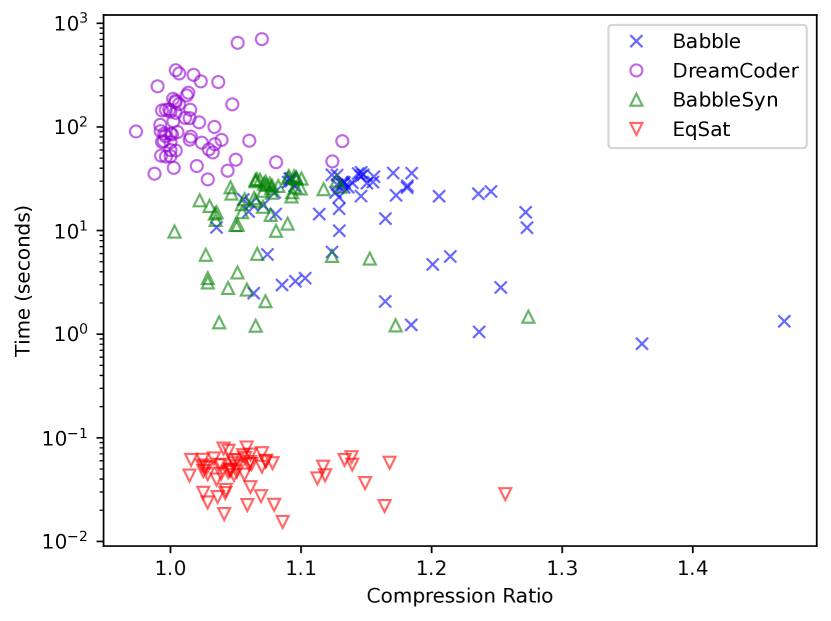
(a) List domain

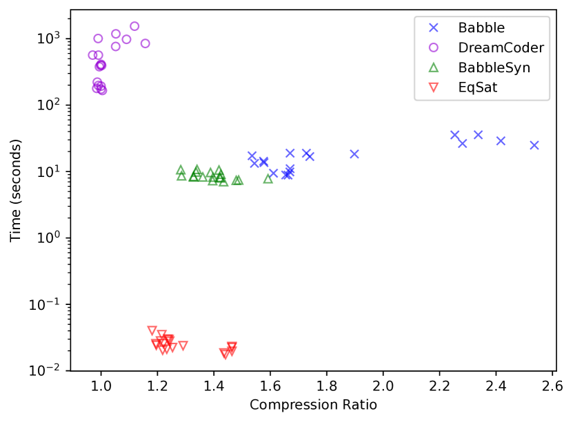
(b) Physics domain

(c) Text domain

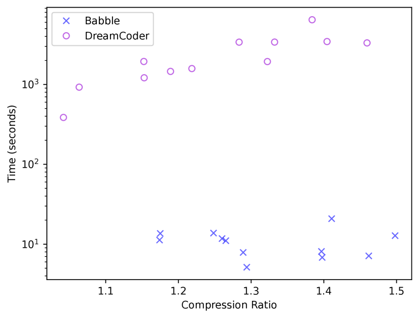
(d) Logo domain

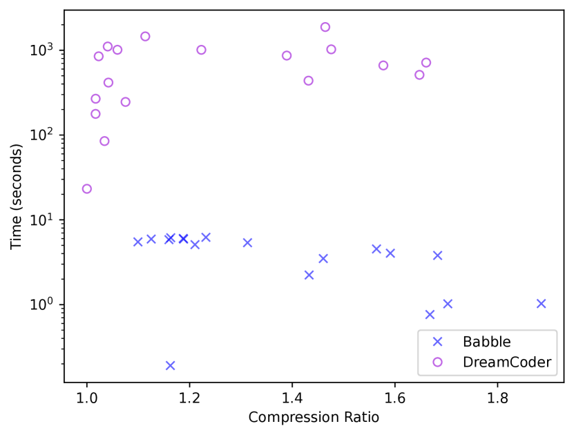
(e) Towers domain

Figure 12. babble consistently achieves better compression ratios than DreamCoder on benchmarks from the DreamCoder domains, and it does so 1–2 orders of magnitude faster. Each marker shows the compression ratio (x-axis) and run time (y-axis) of a benchmark. Each benchmark is one DreamCoder input, i.e., a set of groups of programs as described above. Lower and to the right is better. In the domains where we supplied babble with an equational theory (List and Physics), additional markers show the performance of babble using purely syntactic learning (without equations, “BabbleSyn”) or only equality saturation without library learning (“EqSat”).

To answer RQ 1, we compare to the state-of-the-art DreamCoder tool (Ellis et al., 2021) on its own benchmarks. The DreamCoder benchmarks are suited to its workflow; while the input to a library learning task is conceptually a set of programs (or just one big program), each input to DreamCoder is a set of groups of programs. Each group is a set of programs that are all output from the same program synthesis task (from an earlier part of the DreamCoder pipeline). When compressing a program via library learning, DreamCoder is minimizing the cost of the program made by concatenating the most compressed program from each group together, in other words:

$$\sum_{\textsf{group $g$}}\min_{\textsf{program $p\in g$}}\textsf{cost}(p)$$

DreamCoder takes this approach to give its library learning component many variants of the same program, in order to introduce more shared structure between solution programs across different synthesis problems.

To implement DreamCoder’s benchmarks in babble, we use the e-graph to capture the notion of program variants in a group. Since every program in a group is the output of the same synthesis task, babble considers them equivalent and places them in the same e-class.

Results. We ran babble on five domains from the DreamCoder benchmark suite. The results are shown in Fig. 12. In summary, babble consistently achieves better compression ratios than DreamCoder on benchmarks from the DreamCoder domains, and it does so 1–2 orders of magnitude faster.

The Role of Equational Theory. To answer RQ 2, we again turn to the DreamCoder benchmarks, focusing on the domains where we supplied babble with an equational theory: List and Physics. In these domains, we ran babble in two additional configurations:

• “BabbleSyn” ignores the equational theory, just doing syntactic library learning.

• “EqSat” just optimizes the program using Equality Saturation with the rewrites from the equational theory. This configuration does not do any library learning.

12(a) and 12(b) show the results for these additional configurations, as well as DreamCoder and the normal babble configuration. All babble configurations rely on targeted subexpression elimination to select the final learned library. The “EqSat” configuration is unsurprisingly very fast but performs relatively little compression, as it does not learn any library abstractions. The “BabbleSyn” configuration does indeed compress the inputs, in fact it is still better than DreamCoder in both domains. However, the addition of the equational theory (the “babble” markers in the plots) significantly improves compression and adds relatively little run time, well within an order of magnitude.

6.2. Large-Scale 2d cad Benchmarks

		Without Eqs			With Eqs
Benchmark	Input Size	Out Size	CR	Time (s)	Out Size	CR	Time (s)
Nuts & Bolts	19009	2059	9.23	18.74	1744	10.90	40.75
Vehicles	35427	6477	5.47	79.50	5505	6.44	78.03
Gadgets	35713	6798	5.25	75.07	5037	7.09	82.29
Furniture	42936	10539	4.07	133.25	9417	4.56	110.00
Nuts & Bolts (clean)	18259	2215	8.24	18.12	1744	10.47	40.91

Table 2. Results for running babble on the four large examples from the 2d cad dataset (Wong et al., 2022), both without and with an equational theory. Each row includes the input and output AST sizes, the compression ratio (CR), and babble’s run time in seconds. Fig. 13 plots this data. The final row shows performance on a modified dataset.

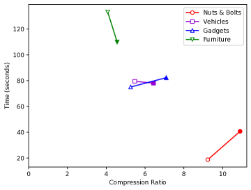
Figure 13. Data from Tab. 2 in scatter plot. Each line segment shows compression ratio and run time for a domain without (hollow marker) and with (solid marker) an equational theory. Using an equational theory improves compression in all cases, and even improves run time in two cases.

The previous section demonstrated that babble’s performance far surpasses the state of the art. In this section, we present and discuss the results of running babble on benchmarks from the 2d cad domain. These benchmarks, taken from Wong et al. (2022), are significantly larger (roughly 10x - 100x) than those from the DreamCoder dataset and out of reach for DreamCoder.

Quantitative Results. Tab. 2 and Fig. 13 show the results of running babble on the benchmarks from the 2d cad domain. The plot in Fig. 13 makes two observations clear. First and relevant for RQ 2, the addition of an equational theory improved all four benchmarks (the solid marker is always to the right of the hollow marker). Second, and perhaps surprisingly, equational theories can sometimes make babble faster! This is consistent with previous observations about equality saturation (Willsey et al., 2021): while equality saturation typically makes an e-graph larger, it can sometimes combine two relevant e-classes into one and reduce the amount of work that some operation over an e-graph must do.

We also observed that the Nuts-and-bolts dataset contains several redundant transformations, like the “scale by 1” featured in the running example of Sec. 2. These redundancies can be useful for finding abstractions in the absence of an equational theory. However, they should not be required in babble since LLMT can introduce the redundancies wherever required. We therefore removed all existing redundant transformations from Nuts-and-bolts and ran babble on the transformed dataset. The results are in the final row of Tab. 2. On the modified dataset, babble achieves identical compression when using the equational theory, but without the equations it performs worse than on the unmodified dataset.

Qualitative Evaluation.

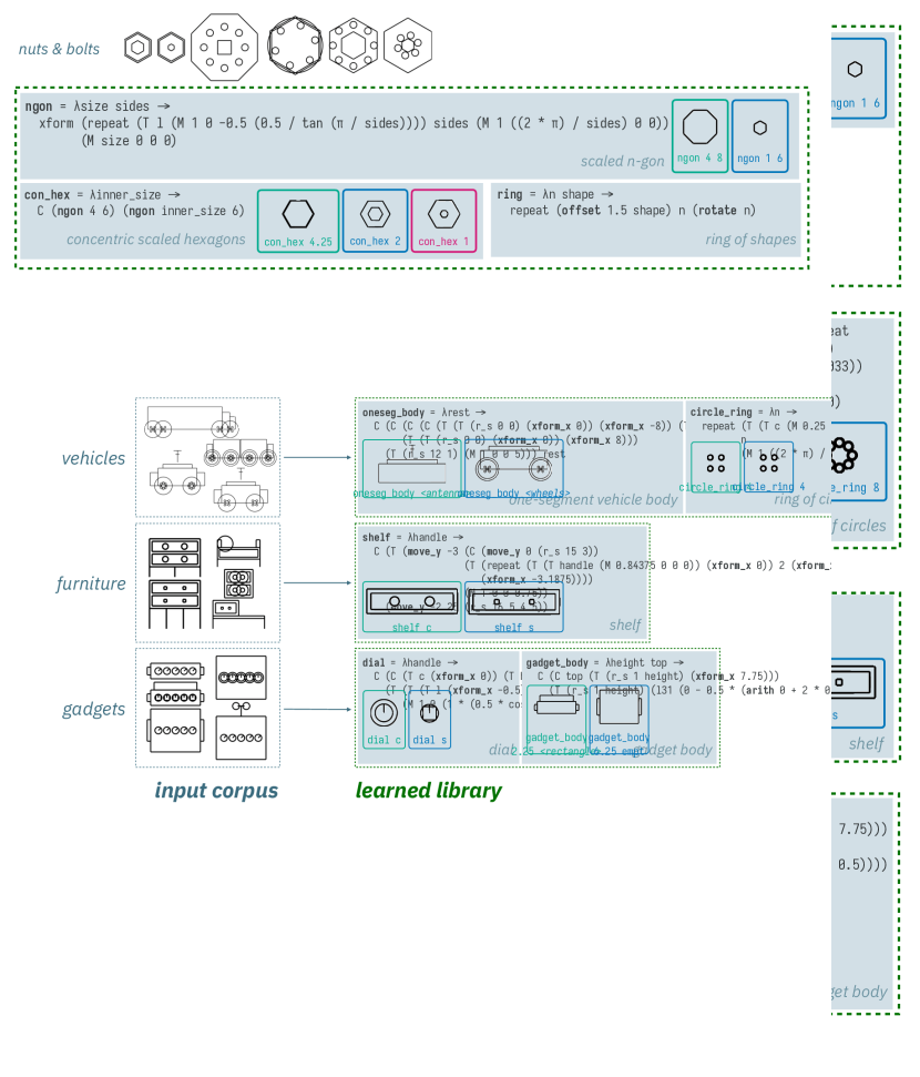
Figure 14. A selection of evaluated programs from each of the domains in the 2d cad dataset, along with a selection of functions that babble learns within the first ten rounds for each domain. Bolded functions represent learned abstractions. Note this figure uses the concrete syntax from the 2d cad dataset; it is similar to the simplified form shown in the overview. We named the learned functions and their parameters for clarity.

Fig. 14 highlights a sample of abstractions that babble discovered from the 2d cad benchmarks. We ran babble on each of the benchmarks and applied the learned abstractions on a few input programs to visualize their usage. Questions about usability and readability of learned libraries are difficult to answer without rigorous user studies which we leave for future work. Nevertheless, Fig. 14 shows that babble identifies common structures that are similar across different benchmarks, which makes its output easier to reuse and interpret.

First, we revisit the Nuts-and-bolts example from Sec. 1: Fig. 14 shows that babble learns the scaled polygon (ngon) abstraction which is applicable to several programs in the dataset. We also see that babble consistently finds a similar abstraction representing a “ring of shapes” for both Nuts-and-bolts and Vehicles. Finally, as the Gadgets example shows, babble finds abstractions for both the entire model as well as its components. In this case, it learned the function gadget_body that abstracts the entire outer shape, and it also learned dial that abstracts the handles of the outer shape.

7. Related Work

babble is inspired by work on library learning, specifically the DreamCoder line of work, as well as equality saturation-based program synthesis and decompilation.

DreamCoder. DreamCoder (Ellis et al., 2021) is a program synthesizer that learns a library of abstractions from solutions to a set of related synthesis tasks. The library is intended to be used for solving other similar synthesis tasks. DreamCoder uses version spaces (Mitchell, 1977; Lau et al., 2001) to compactly store a large set of programs and leverages ideas from e-graphs (such as e-matching) but only for exploring the space of refactorings of the original program using the candidate libraries, not for making library learning robust to syntactic variation. Our evaluation shows that babble can find more optimal abstractions faster than DreamCoder.

DreamCoder has sparked several direction of follow-up work that attempt to improve the efficiency of its library learning procedure and the quality of the learned abstractions. One of them is by Wong et al. (2021), which uses natural language annotations and a neural network to guide library learning. Another one is Stitch (Bowers et al., 2023), which was developed concurrently with this work and is the most closely related to babble; we discuss Stitch in some detail below.

Stitch. The core difference between the two approaches is that Stitch focuses on improving efficiency of purely syntactic library learning, whereas babble attempts to improve its expressiveness by adding equational theories. While babble separates library learning into two phases—candidate generation via anti-unification and candidate selection via e-graph extraction—the Stitch algorithm interleaves the generation and selection phases in a branch-and-bound top-down search. Starting from the “top” pattern $X$, Stitch gradually refines it until further refinement does not pay off. To quickly prune suboptimal candidate patterns, Stitch computes an upper bound on their compression by summing up the compression at each match of this pattern in the corpus (this bound is imprecise because it does not take into account that matches might overlap). For candidates that are not pruned this way, Stitch computes their true compression by searching for the optimal subset of matches to rewrite, a so-called “rewrite strategy”. babble’s extraction algorithm can be seen as a generalization of Stitch’s rewrite strategy: while the former searches over both subsets of patterns and how to apply them to the corpus at the same time, the latter considers a single pattern at a time and only searches for the best way to apply it. Since the search space in the former case is much larger, babble uses a beam search approximation, while in Stitch the rewrite strategy is precise. To sum up, the main pros and cons of the two approaches are:

• babble can learn libraries modulo equational theories, while Stitch cannot;

• Stitch provides optimality guarantees for learning a single best abstraction at a time, while babble can learn multiple abstractions at once, but sacrifices theoretical optimality.

Other Library Learning Techniques. Knorf (Dumancic et al., 2021) is a library learning tool for logic programs, which, like babble, proceeds in two phases. Their candidate generation phase is similar to the upper bound computation in Stitch, while their selection phase uses an off-the-shelf constraint solver. It would be interesting to explore whether their constraint-based technique can be generalized beyond logic programs.

Other work develops limited forms of library learning, where only certain kinds of sub-terms can be abstracted. For example, ShapeMod (Jones et al., 2021) learns macros for 3D shapes represented in a DSL called ShapeAssembly, and only supports abstracting over numeric parameters, like dimensions of shapes. Our own prior work (Wang et al., 2021) extracts common structure from graphical programs, but only supports abstracting over primitive shapes and applying the abstraction at the top level of the program. Such restrictions make the library learning problem more computationally tractable, but limit the expressiveness of the learned abstractions.

There are several neural program synthesis tools (Shin et al., 2019; Iyer et al., 2019; Dechter et al., 2013; Lázaro-Gredilla et al., 2018) that learn programming idioms using statistical techniques. Some of these tools have used “explore-compress” algorithms (Dechter et al., 2013) to iteratively enumerate a set of programs from a grammar and find a solution that exposes abstractions that make the set of programs maximally compressible. This is similar to common subexpression elimination which babble uses for guiding extraction.

Loop rerolling. Loop rerolling is related to library learning in that it also aims to discover hidden structure in a program, except that this structure is in the form of loops. A variety of domains have used loop rerolling to infer abstractions from flat input programs. In hardware, loop rerolling is used to optimize programs for code size (Rocha et al., 2022; Stiff and Vahid, 2005; Su et al., 1984). In many of these tools, the compiler first unrolls a loop, applies optimizations, then rerolls it — the compiler therefore has structural information about the loop that can be used for rerolling (Rocha et al., 2022). The graphics domain has used loop-rerolling to discover latent structure from low-level representations. CSGNet (Sharma et al., 2017) and Shape2Prog (Tian et al., 2019) used neural program generators to discover for loops from pixel- and voxel-based input representations. (Ellis et al., 2017) used program synthesis and machine learning to infer loops from hand-drawn images. Szalinski (Nandi et al., 2020) used equality saturation to automatically learn loops in the form of maps and folds from flat 3D CAD programs that are synthesized by mesh decompilation tools (Nandi et al., 2018). WebRobot (Dong et al., 2022) has used speculative rewriting for inferring loops from traces of web interactions. Similar to babble (and unlike Szalinski), WebRobot finds abstractions over multiple input traces.

Applications of Anti-Unification. Anti-unification is a well-established technique for discovering common structure in programs. It is the core idea behind bottom-up Inductive Logic Programming (Cropper and Dumancic, 2022), and has also been used for software clone detection (Bulychev et al., 2010), programming by example (Raza et al., 2014), and learning repetitive code edits (Meng et al., 2013; Rolim et al., 2017). It is possible that these applications could also benefit from babble’s notion of anti-unification over e-graphs to make them more robust to semantics-preserving transformations.

Synthesis and Optimization using E-graphs. While traditionally e-graphs have been used in SMT solvers for facilatiting communication between different theories, several tools have demonstrated their use for optimization and synthesis. Tate et al. (2009) first used e-graphs for equality saturation: a rewrite-driven technique for optimizing Java programs with loops. Since then, several tools have used equality saturation for finding programs equivalent to, but better than, some input program (Willsey et al., 2021; Panchekha et al., 2015; Yang et al., 2021; Nandi et al., 2020; VanHattum et al., 2021; Wang et al., 2020; Wu et al., 2019). babble uses an anti-unification algorithm on e-graphs (together with domain specific rewrites), which prior work has not shown. Additionally, prior work has either used greedy or ILP-based extraction strategies, whereas babble uses a new targeted common subexpression elimination approach which we believe can be used in many other applications of equality saturation, especially given its amenability to approximation via beam search.

8. Conclusion and Future Work

We presented library learning modulo theory (LLMT), a technique for learning abstractions from a corpus of programs modulo a user-provided equational theory. We implemented LLMT in babble. Our evaluation showed that babble achieves better compression orders of magnitude faster than the state of the art. On a larger benchmark suite of 2d cad programs, babble learns sensible functions that compress a dataset that was—until now—too large for library learning techniques.

LLMT and babble present many avenues for future work. First, our evaluation showed that equational theories are important for achieving high compression, but these must be provided by domain experts. Recent work in automated theory synthesis like Ruler (Nandi et al., 2021) or TheSy (Singher and Itzhaky, 2021) could aid the user in this task. Second, LLMT uses e-graph anti-unification to generate promising abstraction candidates, but this approach is incomplete and misses some patterns that could achieve better compression. An exciting direction for future work is to combine LLMT with more efficient top-down search from Stitch (Bowers et al., 2023). This is challenging because Stitch crucially relies on the ability to quickly compute an upper bound on the compression of a given pattern by summing up the local compression at each of its matches in the corpus. This upper bound does not straightforwardly extend to e-graphs because in an e-graph different matches of a pattern may come from different syntactic variants of the corpus, and one needs to trade-off the compression from abstractions against the size difference between different syntactic variants.

Appendix A Proofs

Proposition A.1.

The language of compressed terms is strongly normalizing.

Proof.

Consider evaluating $\hat{t}$ in applicative order (leftmost innermost). In this case, any left-hand size of a $\beta$-reduction has no inner $\beta$-redexes. Since in our language a $\lambda$-abstraction can only be on the left-hand side of a $\beta$-redex, it means that expression being reduced has no inner $\lambda$-abstractions. For that reason, the number of $\lambda$-abstractions in an expression strictly decreases with every $\beta$-step (the sole one in the reduced redex disappears, and all other $\lambda$-abstractions are outside of the reduced redex, and hence unchanged). ∎

Lemma A.2.

Given a $\kappa$-step $\hat{t}_{1}\rightarrow^{\kappa(p^{\prime})}_{1}\hat{t}_{2}$ if a pattern $p$ has $N$ matches in $\hat{t}_{2}$, it also has at least $N$ matches in $\hat{t}_{1}$.

Proof.

There are four cases for what $p$ can match in $\hat{t}_{2}$:

• a subterm that does not overlap with the newly introduced $\beta$-redex: in this case, the match is unaffected by the $\kappa$-step;

• a subterm inside an actual argument of the $\beta$-redex: this actual argument becomes a sub-term of $\hat{t}_{1}$;

• a sub-term inside the body of the $\beta$-redex: $\hat{t}_{1}$ has a sub-term that is more specific than the body, and hence still matches $p$;

• a sub-term that includes the entire $\beta$-redex inside: since $p$ is first order, it cannot mention the redex, so the redex must be contained entirely inside the substitution; hence again the match is unaffected by the $\kappa$-step.

∎

Theorem A.3 (Soundness and Completeness of Pattern-Based Library Learning).

For any term $t\in\mathcal{T}(\Sigma)$ and compressed term $\hat{t}\in\hat{\mathcal{T}}(\Sigma,\mathcal{X})$:

(Soundness):

If $t$ compresses into $\hat{t}$, then $\hat{t}$ evaluates to $t$: $\forall\mathcal{P}.t\rightarrow^{\kappa(\mathcal{P})}\hat{t}\Longrightarrow\hat{t}\rightarrow^{\beta}t$.

(Completeness):

If $\hat{t}$ is a solution to the (global) library learning problem, then $t$ compresses into $\hat{t}$ using only patterns that have a match in $t$: $\hat{t}\in\operatorname*{arg\,min}_{\hat{t}^{\prime}\rightarrow^{\beta}t}\mathsf{size}(\hat{t}^{\prime})\Longrightarrow t\rightarrow^{\kappa(\mathcal{P})}\hat{t}$, where $\mathcal{P}=\{p\in\mathcal{T}(\Sigma,\mathcal{X})\mid t^{\prime}\in\mathsf{subterms}(t),t^{\prime}\sqsubseteq p\}$.

Proof.

The soundness is trivial because inverting any $\kappa$-rewrite gives a valid $\beta$-reduction.

The other direction (completeness) is more involved. First let us prove that $\hat{t}$ can be obtain by any compression, regardless of whether the patterns occur in $t$. This is non-trivial because inverting a $\beta$-reduction $(\lambda\overline{X}\ \mathbf{\shortrightarrow}\ \hat{t}_{1})\ \overline{\hat{t}_{2}}\rightarrow^{\beta}_{1}\hat{t}^{\prime}$ does not always correspond to a well-form $\kappa$-step, for two reasons: (a) $\hat{t}_{1}$ itself contains $\lambda$-abstractions (and hence does not correspond to a pattern); (b) $\overline{X}\neq\mathsf{vars}(\hat{t}_{1})$. To overcome point (a), note that in an applicative evaluation, both $\hat{t}_{1}$ and $\hat{t}_{2}$ contain no $\beta$-redexes (and hence no $\lambda$-abstractions). Hence $\hat{t}_{1}$ is a valid pattern.

For point (b), there are two cases: either (1) $\mathsf{vars}(\hat{t}_{1})\subsetneq\overline{X}$ or (2) $\mathsf{vars}(\hat{t}_{1})\supsetneq\overline{X}$. Consider case (1). In this case, the compressed term $\hat{t}$ has $\lambda$-bindings that are not used in their bodies. Such a term cannot possibly be minimal. Removing unused bindings makes each individual $\beta$-redex smaller and cannot remove sharing, so it always makes the overall term smaller as well.

Now consider case (2). This means that $\lambda\overline{X}\ \mathbf{\shortrightarrow}\ \hat{t}_{1}$ has free variables, which must be defined in outer $\lambda$-abstractions. However, using such a $\lambda$-abstraction contradicts the assumption that we are only interested in global library learning.

Finally, let us prove that all patterns used in the compression have a match in $t$. Consider a compression $t=\hat{t}_{0}\rightarrow^{\kappa(p_{1})}_{1}\hat{t}_{1}\dots\rightarrow^{\kappa(p_{n})}_{1}\hat{t}_{n}=\hat{t}$. Clearly, each pattern $p_{i}$ has a match in the (compressed) term $\hat{t}_{i-1}$, by definition of the $\kappa$-rewrite. Hence, it also occurs in $t$, by induction using Lemma A.2. ∎

Appendix B Additional Experiments

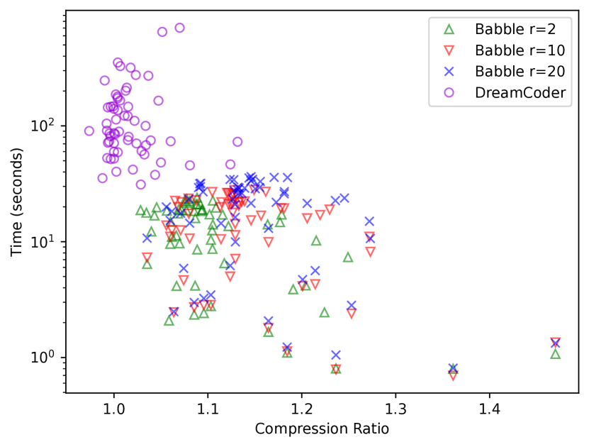
(a) List domain

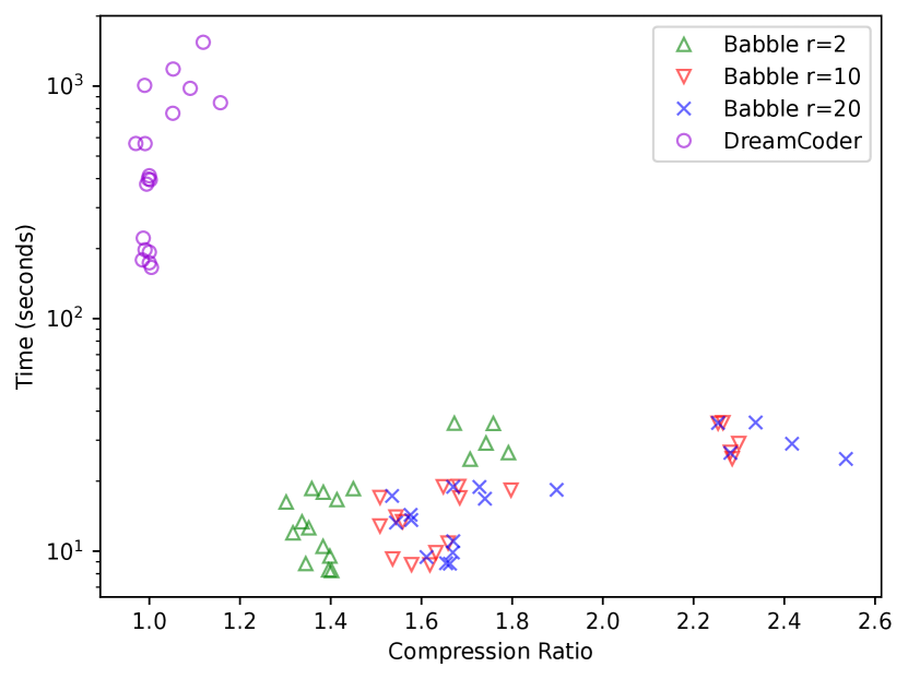
(b) Physics domain

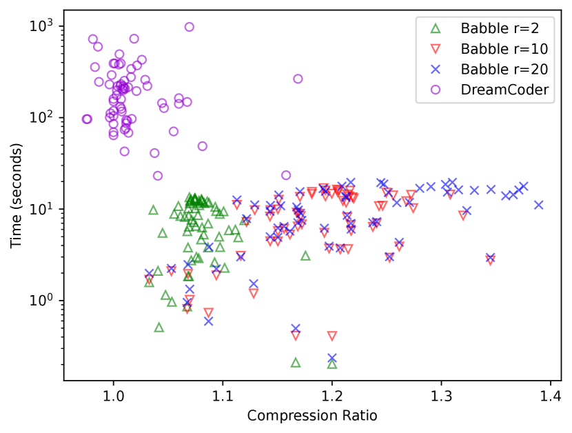
(c) Text domain

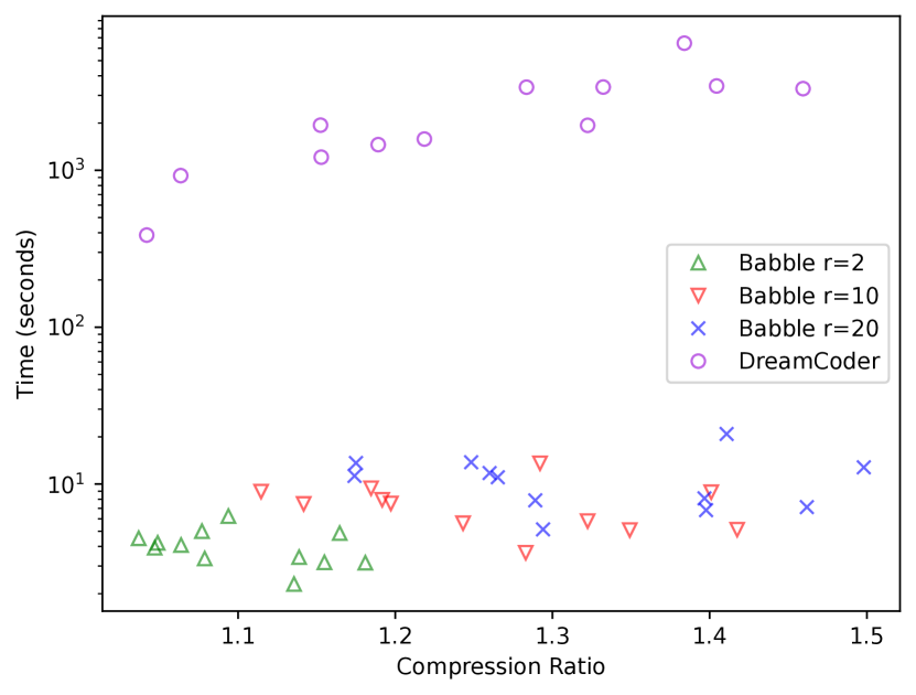
(d) Logo domain

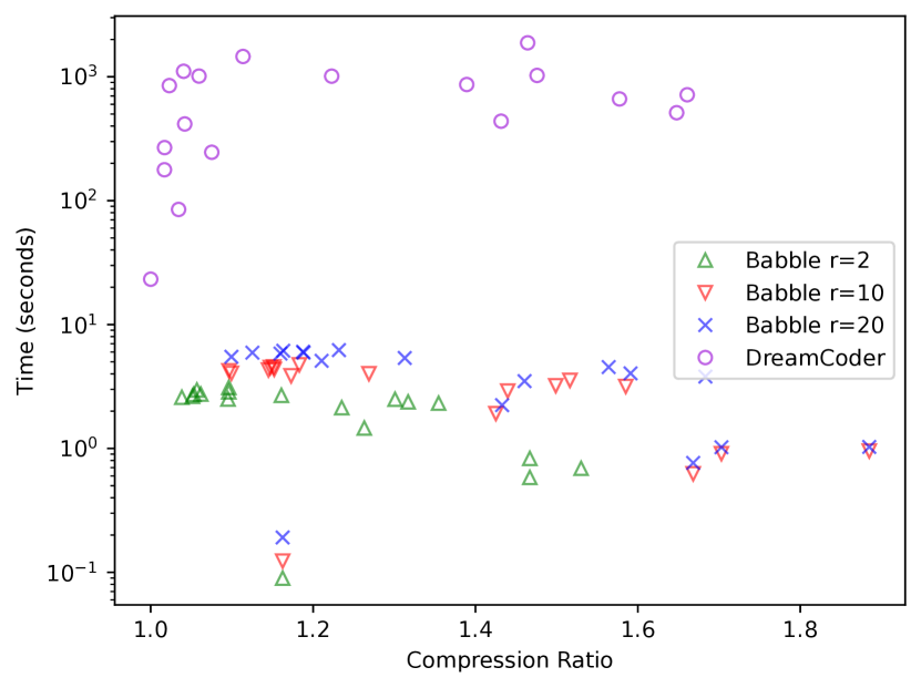
(e) Towers domain

Figure 15. babble’s default configuration runs for 20 rounds (r=20) to learn additional library functions. This plot shows the data from Fig. 12, but with additional babble configuration running fewer rounds. With fewer rounds, babble runs faster but compresses worse.