DP-RAFT: A Differentially Private Recipe for Accelerated Fine-Tuning

Abstract

A major direction in differentially private machine learning is differentially private fine-tuning: pretraining a model on a source of "public data" and transferring the extracted features to downstream tasks. This is an important setting because many industry deployments fine-tune publicly available feature extractors on proprietary data for downstream tasks. In this paper, we carefully integrate techniques, both new and from prior work, to solve benchmark tasks in computer vision and natural language processing using differentially private fine-tuning. Our key insight is that by accelerating training with the choice of key hyperparameters, we can quickly drive the model parameters to regions in parameter space where the impact of noise is minimized. We obtain new state-of-the art performance on CIFAR10, CIFAR100, FashionMNIST, STL10, and PersonaChat, including $99\%$ on CIFAR10 for $\varepsilon=1,\delta=1e-5$-DP.

1 INTRODUCTION

As organizations increasingly use machine learning in real world systems to provide insights on the data generated by real users (Team, 2017), issues of user data privacy have risen to the forefront of existing problems in machine learning. Differential privacy (DP) (Dwork et al., 2006) is the de facto standard for privacy preserving statistics. Common algorithms for privately training machine learning models are differentially private stochastic gradient descent (DP-SGD) (Song et al., 2013; Abadi et al., 2016) and differentially private empirical risk minimization (DP-ERM) (Chaudhuri et al., 2011).

While advancements in deep learning can be partially attributed to scaling up the number of model parameters  (Kaplan et al., 2020; Brown et al., 2020), as shown by  (Kurakin et al., 2022; Tramèr and Boneh, 2020; Yu et al., 2021b; Shen et al., 2021) increasing the number of model parameters in DP-SGD often has an adverse impact on the privacy-utility tradeoff due to the curse of dimensionality present in DP-SGD. Briefly, the "curse" is that the magnitude of the noise added scales with $\sqrt{d}$ the square root of the number of parameters, and because the signal does not scale with the number of parameters, the signal to noise ratio (SNR) suffers at scale. The curse of dimensionality has prevented SOTA DP-SGD benchmarks, such as training from scratch on CIFAR10 and MNIST variants, from improving at the same pace as non-private training. However, we can achieve this performance with private fine-tuning. Training large models with unsupervised or self-supervised learning on massive datasets, and then transferring the learned features to smaller models on downstream tasks via fine-tuning, is increasingly common to achieve good performance on benchmark tasks and in industry applications (Brown et al., 2020). We produce a new recipe for differentially private fine-tuning that can recover the same performance as non-private fine-tuning by carefully integrating techniques from prior work that individually have not reproduced non-private performance (De et al., 2022; Bu et al., 2022; Cattan et al., 2022; Li et al., 2021).

Table 1: We compare the best private and best non-private test accuracy performances of DP-RAFT to prior work using models pretrained on ImageNet-21k and fine-tuned on CIFAR10 and CIFAR100. Full results are in Section 3

Model	Dataset	$\varepsilon=0.1$	$\varepsilon=1$	$\varepsilon=\infty$	Gap ($1-\infty$)
DP-RAFT	CIFAR10	98.65	99.00	99.00	0.00
	CIFAR100	72.39	89.81	91.57	1.76
SOTA (Mehta et al., 2022a)	CIFAR10	95.8	96.3	96.6	0.3
	CIFAR100	78.5	82.7	85.29	2.59

To achieve the desired privacy guarantees, fine-tuning with DP-SGD requires selecting the appropriate values for several hyperparameters. These hyperparameters include the learning rate schedule, the clipping bound, the batch size, and the amount of noise to add at each iteration. Prior work has either fixed these hyperparameters or performed an extensive search to find the best values (De et al., 2022). In this work, we propose DP-RAFT, a simple yet effective step-by-step recipe that automatically selects the hyperparameters to fine-tune a model with DP-SGD. Our method is based on the observation that adding noise to the gradients can perturb the optimization trajectory, and it is this perturbation that degrades performance. We propose to use gradient descent with momentum to take many large steps in the direction of the gradients, so that the model parameters can reach regions in parameter space where adding noise does not perturb the optimization trajectory. We evaluate DP-RAFT on four benchmark computer vision tasks (CIFAR10, CIFAR100, STL10, FashionMNIST) and report new state-of-the-art results for $\varepsilon\in[0.01,1.0]$, and also provide results for PersonaChat, an NLP task. We notably recover the same performance as non-private fine-tuning for CIFAR10 (99 $\%$) for $\varepsilon=1,\delta=1e-5$, and come within $0.1\%$ accuracy of non-private performance on FashionMNIST and STL10. An abbreviated version of our key results is given in Table. 1 As a part of this empirical evaluation, we open-source our code that includes a 100-line script to reproduce our experiments as well as implementations of a number of techniques proposed by prior work.

2 RELATED WORK

In this section we provide a brief overview of differential privacy, DP-SGD and prior work on fine-tuning pretrained feature extractors with differential privacy. We provide insight onto the key gaps between prior work and this work, and include a detailed treatment of concurrent work.

2.1 Differential Privacy

Differential privacy (Dwork et al., 2006) is the gold standard for data privacy. It is formally defined as below:

Definition 2.1 (Differential Privacy).

A randomized mechanism $\mathcal{M}$ with domain $\mathcal{D}$ and range $\mathcal{R}$ preserves $(\varepsilon,\delta)$-differential privacy iff for any two neighboring datasets $D,D^{\prime}\in\mathcal{D}$ and for any subset $S\subseteq\mathcal{R}$ we have:

$$\Pr[\mathcal{M}(D)\in S]\leq e^{\varepsilon}\Pr[\mathcal{M}(D^{\prime})\in S]+\delta$$ (1)

where $D$ and $D^{\prime}$ are neighboring datasets if they differ in a single entry, $\varepsilon$ is the privacy budget and $\delta$ is the failure probability.

2.2 DP-SGD

Stochastic gradient descent (SGD) performs the following update during non-private training:

$$w^{(t+1)}=w^{(t)}-\frac{\eta_{t}}{|B_{t}|}\sum_{i\in B_{t}}\nabla\ell(x_{i},w^{(t)})$$

where $\eta_{t}$ is the learning rate at iteration $t$, and we update the weights with the loss on the batch $B_{t}$ of size $|B_{t}|$ sampled at iteration $t$. (Abadi et al., 2016) propose the differentially private stochastic gradient descent (DP-SGD) algorithm to train models under a differential privacy guarantee, which adds steps to SGD: (1) gradient clipping to bound sensitivity, where the gradient per each training sample is clipped to make sure its norm is no larger than the clipping bound; (2) noise addition to achieve DP guarantees, where a random Gaussian noise is added to gradient before gradient descent. The new update can be written as:

$$w^{(t+1)}=w^{(t)}-\frac{\eta_{t}}{|B_{t}|}\left(\sum_{i\in B_{t}}\frac{1}{\text{C}}\textbf{clip}_{\text{C}}(\nabla\ell(x_{i},w^{(t)}))+\sigma\xi\right)$$ (2)

where $\textbf{clip}_{\text{C}}(\nabla\ell(x_{i},w^{(t)}))=\frac{C\times\nabla\ell(x_{i},w^{(t)})}{\max(C,||\nabla\ell(x_{i},w^{(t)})||_{2})}$, $\xi\sim\mathcal{N}(0,1)$ is noise sampled from a $d$-dimensional Gaussian distribution, and $\sigma$ is the standard deviation of the added noise. Note that the clipping parameter $C$ can be chosen to a range of possible values, and as long as the clipping threshold is smaller than the norm of every per-sample gradient, this is equivalent to just adjusting the learning rate (De et al., 2022).

Short review of fine-tuning efforts with DP-SGD.

(De et al., 2022; Cattan et al., 2022) propose the use of a number of techniques when fine-tuning a ResNet pretrained on ImageNet on CIFAR10/CIFAR100. The peak accuracy of $96.7\%$ accuracy is achieved for $(8,10^{-5})$-DP using a myriad of these techniques, and for $\varepsilon=1$ they get $95.0\%$ accuracy. A key takeaway from this line of work is the use of large batch sizes and initializing the weights to small values near-zero to standardize training. However, they use ResNet architectures rather than modern vision transformers, and we find that other techniques that they use such as data augmentation, fine-tuning the embedding layer, and weight averaging do not always improve performance.  (Mehta et al., 2022b) propose differentially private transfer learning at the scale of ImageNet, using large-scale models with large batches.  Bu et al. (2022) report better results of $(\varepsilon=1,96.7\%)$, with GDP and Poisson subsampling, tuning the entire network. They fine-tune modern vision transformer architectures, thus producing massive performance improvements, but we crucially observe that updating all parameters incurs the curse of dimensionality and counter-intuitively, it is better to only update the last layer.  (Radford et al., 2021) shows that a sufficiently sophisticated pretrained model can achieve SOTA performance on CIFAR10 and other benchmark computer vision tasks with zero-shot learning, i.e. ($\varepsilon=0$)-DP, so intuitively similar performance should be well within the reach of DP fine-tuning. Besides vision tasks, (Li et al., 2021) and (Yu et al., 2021a) provide methods for fine-tuning large language models under DP-SGD by proposing new clipping methods to mitigate the memory burden of per-sample gradient clipping. However, they do not achieve performance comparable to non-private models when fine-tuning a pretrained model on the PersonaChat dataset. We adapt their techniques to the hyperparameter settings that we show are optimal for DP fine-tuning, and produce similar performance to non-private fine-tuning on the PersonaChat dataset.

Concurrent Work.

Most recently,  (Mehta et al., 2022a) provide an extensive evaluation of various alternatives to DP-SGD for transfer learning. As the computational burden of fine-tuning the last layer of a pre-trained model is relatively low, they investigate second-order DP algorithms including DP Newton for logistic regression and DP Least Square for linear regression and find that second-order information is helpful to improve the model utility in private training. They further propose DP-FC (DP-SGD with Feature Covariance) to avoid the computation of Hessian over iterations. We also focus on training the linear layer on features extracted from a model pre-trained on a public dataset. However, the goal of our paper is to focus on the common DP-SGD setting and provide a recipe for accelerated finetuning. We note that all numbers we report for models pretrained on ImageNet-21k using first-order methods surpass those in (Mehta et al., 2022a), but for sufficiently small values of $\varepsilon$ on harder datasets, specifically $\varepsilon\leq 0.01$ on CIFAR100 the second-order methods they propose provide better performance.

3 Evaluation

In this section, we present DP-RAFT, a simple recipe for differentially private (DP) fine-tuning and provide results on four image classification tasks and one next-word prediction task.

DP-RAFT: A Differentially Private Recipe for Accelerated Fine-tuning.

We provide pseudocode for DP-RAFT in Alg. 1, full code and summarize the improvement of each step in Table 2. At a high level, we want to ensure that the noisy updates of differentially private gradient descent point in the direction of the optimal solution, by maximizing the signal-to-noise ratio of updates and accelerating optimization.

1) Extract features from a private dataset using an open source feature extractor pretrained on a public dataset.

2) Zero-initialize a classifier that maps features to classes: by minimizing the number of parameters, we mitigate the curse of dimensionality.

3) Apply a new linear scaling rule to create a training schedule: we select the optimal hyperparameters for a given privacy budget using trials with much smaller privacy budgets.

4) Compute the full batch gradient: this optimizes the signal-to-noise ratio of the update and enables using large step sizes.

5) Enforce sensitivity by clipping per-sample gradients to unit norm: this keeps step sizes large without introducing significant bias into the gradient.

6) Use privacy loss variable accounting (Gopi et al., 2021) to calibrate Gaussian noise for the given privacy budget and add noise to the gradient: this enables budgeting for small values of $\varepsilon$ without underestimating privacy expenditure.

7) Take a step of size given by (3) using momentum (Qian, 1999): large step sizes with acceleration quickly increase the size of the model.

8) Repeat steps 4-7 according to the number of iterations given by (3): training for many iterations provides good performance for all values of $\varepsilon$.

9) Take a final step with the same learning rate in the direction of the momentum buffer: the momentum is private by post-processing, so taking a free step further boosts performance.

We ablate and provide intuition for each step in the following sections.

Algorithm 1 Differentially Private Recipe for Accelerated Fine-Tuning (DP-RAFT)

  Inputs: Private dataset $\mathcal{D}$, open source feature extractor F, number of classes $C$, privacy budget $\varepsilon$

  Extract features from $\mathcal{D}$ using F: $\mathcal{X}=\text{F}(\mathcal{D})$

  Zero-initialize classifier $w\leftarrow 0_{C\times d}$

  Apply the linear scaling rule to obtain a training schedule $(\eta,T)$ given $\varepsilon$

  Use privacy loss variable accounting to calibrate noise parameter $\sigma$ given $\varepsilon$

  for $i=1,2,\dots,T$ do

     Compute full-batch gradient according to Eq. 2 $\nabla^{(i)}=\frac{1}{|D|}\left(\sum_{i\in D}\textbf{clip}_{1}(\nabla\ell(x_{i},w^{(i)}))+\sigma\xi\right)$

     Take a step with momentum: $v^{(i)}\leftarrow 0.9\cdot v^{(i-1)}+\nabla^{(i)}$, $w^{(i)}\leftarrow w^{(i-1)}-\eta v^{(i)}$

  end for

  Take a final step in the direction of the momentum buffer: $w\leftarrow w-\eta v$

  Output: Private classifier $w$

Table 2: Improvements obtained by following the Recipe for Private Fine-Tuning. Details for ablations can be found in the corresponding paragraphs.

Method	Baseline	Baseline Accuracy	Improvement
New Linear Scaling Rule	Early Stopping (Mehta et al., 2022a)	80.7	4.29
Classifier (no bias)	(Mehta et al., 2022b)	71.3	0.36
Zero Initialization	Random Initialization (De et al., 2022)	64.85	6.81
Gradient Descent	SGD(Batch=4096) (De et al., 2022)	70.2	1.46
Momentum ($\rho=0.9$)	$\rho=0$ (Bu et al., 2022)	69.02	2.09
PLV Accounting	RDP (De et al., 2022)	68.43	3.23
Unit Clipping (C=1)	$C\ll 1$ (Mehta et al., 2022a)	71.2	0.46
Free Step	N/A	71.11	0.55

Table 3: We compare the best private and best non-private performances of all models on all datasets. We use the same grid search settings for all experiments. When ’Prior SOTA’ is listed, we use results from their models fine-tuned on ImageNet-21k.

Model	Dataset	$\varepsilon=1$	$\varepsilon=\infty$	Gap
beitv2-224	CIFAR10	99.00	99.00	0.00
	CIFAR100	89.81	91.57	1.76
	FashionMNIST	91.38	91.53	0.15
	STL10	99.71	99.81	0.10
convnext-384	CIFAR10	96.94	97.22	0.28
	CIFAR100	83.69	86.59	2.90
	FashionMNIST	90.43	91.13	0.77
	STL10	99.61	99.71	0.10
beit-512	CIFAR10	98.27	98.51	0.24
	CIFAR100	87.31	90.08	2.77
	FashionMNIST	90.87	91.6	0.73
	STL10	99.62	99.78	0.16
vit-large-384	CIFAR10	98.29	98.44	0.40
	CIFAR100	86.18	89.72	3.54
	FashionMNIST	90.58	91.37	0.79
	STL10	99.62	99.76	0.14
Prior SOTA (Mehta et al., 2022a)	CIFAR10	96.3	96.6	0.3
	CIFAR100	82.7	85.29	2.59

Models.

We evaluate five models: two masked-image modeling transformers, beit (Bao et al., 2021) and beitv2 (Peng et al., 2022), their backbone architecture ViT (Dosovitskiy et al., 2020) at both the base and large scales, and the pure convolutional architecture convnext (Liu et al., 2022). All models are pretrained on ImageNet-21k (Deng et al., 2009). These models span a range of input resolutions: beitv2 (224x224), convnext, vit-base, vit-large (384x384), and beit (512x512) and we upsample images to the necessary input size.

Datasets.

For image classification we use CIFAR10, CIFAR100 (Krizhevsky et al., 2009), FashionMNIST (Xiao et al., 2017), STL10 (Coates et al., 2011) for private fine-tuning. For next word generation we use PersonaChat (Zhang et al., 2018a). Similar to prior work, these fine-tuning datasets do not contain any sensitive data.

Availability.

Our results tune open source models from the PyTorch timm package (Wightman, 2019) using existing privacy accounting from (Gopi et al., 2021) and per-sample clipping code in (Yousefpour et al., 2021), requiring no new algorithms or pretraining. As a result, our key results can be reproduced in a matter of minutes.

A New Linear Scaling Rule.

We propose a new linear scaling rule for the remaining hyperparameters: increase either the learning rate $\eta$ or number of epochs $T$ linearly with $\varepsilon$ so that the total step size $r=\eta\times T$ is linear in $\varepsilon$. In Fig. 1 we report that following this rule produces new state-of-the-art results for all values of $\varepsilon$, shown in Table 3. Fig. 2 validates that this rule is robust: we can move from one set of hyperparameters to another similarly performing set of hyperparameters by increasing the number of iterations $T$ by a constant factor and decreasing the learning rate $\eta$ by the same factor (or vice versa). Consider the second heatmap in Fig. 2: $(\eta=0.5,T=10)=70.17$ and $(\eta=0.1,T=50)=71.16$ perform similarly. We zoom in on CIFAR100 in Fig. 3 and show the improvement from linearly scaling $r$ with $\varepsilon$. Although our evaluation focuses on the beit models trained with self-supervised pretraining, to compare the effectiveness of linear scaling against the hyperparameter selection strategies used in prior work we apply linear scaling to the ViT used in  (Mehta et al., 2022a). Using hyperparameters corresponding to $r=20$, we recover performance of $82.7\%$ for $\varepsilon=1$, a $2\%$ improvement over the early stopping strategy employed in  (Mehta et al., 2022a) for DP-Adam and in fact reproducing the performance of their proposed second-order method. This suggests that, at least for this relatively larger value of $\varepsilon$, first-order methods are competitive with second-order methods. Full heatmaps for all datasets and models can be found in the Appendix.

Our key insight is that this new linear scaling rule turns existing intuition on noisy optimization into an actionable strategy for hyperparameter selection.

The New Linear Scaling Rule is Intuitive.

We provide an intuitive explanation for the new linear scaling rule here. First note that the classification accuracy of a linear model is scale-invariant; the optimal solution of GD($r$) is $\theta^{\prime}=\theta^{*}/\left\lVert\theta^{*}\right\rVert\times r$: the projection of $\theta^{*}$ onto $B_{r}$, the ball of radius $r$, and for linear models, the performance (top-1 accuracy) of $\theta^{\prime}$ is the same as the performance of $\theta^{*}$: $\operatorname*{argmax}_{c}\theta^{\prime}(x)=\operatorname*{argmax}_{c}\theta^{*}(x)\,\forall x$. The critical factor in the success of logistic regression is the angle between the gradient update $\nabla_{i}$ and $\theta^{\prime}$. Let $\text{similarity(i)}=\frac{\nabla_{i}\cdot\theta^{\prime}}{\left\lVert\nabla_{i}\right\rVert\cdot\left\lVert\theta^{\prime}\right\rVert}$. Suppose that $\left\lVert\theta_{i}\right\rVert=\left\lVert\theta^{\prime}\right\rVert\ll 1$, then adding Gaussian noise $\sigma\xi$ where $\xi\sim\mathcal{N}(0,1)$ to the update will significantly decrease the cosine similarity of the updated model and $\theta^{\prime}$. If we decrease $\sigma$, it is easy to see that this mitigates the impact on the trajectory. This is the setting pursued by prior work: by keeping the number of iterations small (Mehta et al., 2022a), we reduce $\sigma$. However, we can equivalently keep $\sigma$ constant and increase the scale of the parameters, and also decrease the impact of noise on the trajectory: $\text{similarity}(\theta_{i}+\sigma\xi,\theta^{\prime})<\text{similarity}(\alpha\cdot\theta_{i}+\sigma\xi,\alpha\cdot\theta^{\prime}),\forall\alpha>1$. Note that by increasing $r$ we scale the optimal solution while keeping its performance identical, and thus optimize the cosine similarity of the noisy update. The linear scaling rule advocates exactly this: increasing the number of iterations and the learning rate linearly increases $r$ but does not linearly increase $\sigma$ due to the composition of Gaussian differential privacy (Gopi et al., 2021), therefore the impact on the optimization trajectory is minimized.

Selecting the Best Model and Training Schedule is Challenging.

There are hundreds of open source models pretrained on ImageNet that can be used as feature extractors, and choosing the best model for the downstream task is critical (Kornblith et al., 2018). A straightforward baseline is to always pick the model with the highest ImageNet top-1 accuracy. However, as we show in Table 4 this greedy baseline does not select the best model for the task. Hyperparameter selection is another critical problem in private fine-tuning, because hyperparameter tuning costs privacy and naive grid search swiftly burns through even generous privacy budgets (Papernot and Steinke, 2021). While our recipe does not use many hyperparameters, we still need to specify the number of training iterations $T$ and the learning rate $\eta$. Prior work generally trains for a small number of iterations with a small learning rate (Bu et al., 2022; Cattan et al., 2022; Mehta et al., 2022a; De et al., 2022), but as we show in Fig. 2 this strategy (corresponding to the top left of the heatmaps) is suboptimal.

Table 4: Comparing four models for DP transfer learning with $\varepsilon=0.1$, we see that choosing the model based on the pretrained accuracy does not typically produce the best model for the task.

Model	Pretraining Accuracy (ImageNet)	CIFAR10	CIFAR100	STL10	FashionMNIST
convnext-384	87.54	96.03	68.38	94.48	87.72
vit-384	87.08	96.84	62.22	80.15	83.65
beitv2-224	87.48	98.65	63.25	81.58	88.87
beit-512	88.60	97.74	72.39	94.1	88.1

(a) Pareto Frontier for $\varepsilon$ vs Test Accuracy

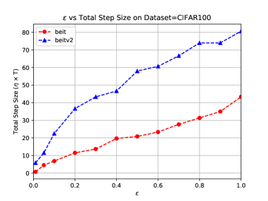
(b) Pareto Frontier for $\varepsilon$ vs Total Step Size

Figure 1: As $\varepsilon$ increases, the optimal value of $\eta\times T$ increases linearly, and test accuracy also increases. The optimal value of $\eta\times T$ for beitv2 increases much faster than beit, and therefore for larger privacy budgets beitv2 outperforms beit.

(a) CIFAR100 Beit

(b) CIFAR100 Beitv2

Figure 2: Heatmaps for beit and beitv2 on CIFAR100; lighter is higher test accuracy. $\varepsilon$ increases from $0.05\rightarrow 1.0$, iterations $T$ increases from $5\rightarrow 100$, and the learning rate $\eta$ increases from $0.05\downarrow 1$. As $\varepsilon$ increases, left to right, the optimal value of $\eta\times T$ increases in accordance with the new linear scaling rule. Prior work has generally operated in the top-left regime, that is often suboptimal.

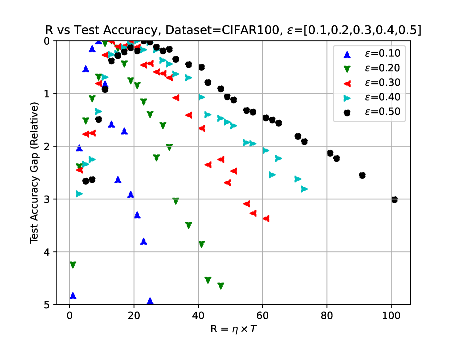
(a) CIFAR100 Beitv2

Figure 3: A scatter plot of $r=\eta\times T$ the linear scaling parameter vs the relative gap in test accuracy; this gap is measured as the difference between the test accuracy at the plotted value of $r$ and the optimal value of $r$. Even though the absolute performance differs greatly, we see that the optimal value of $r$ increases linearly with $\varepsilon$.

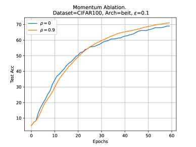
(a) Momentum Acceleration

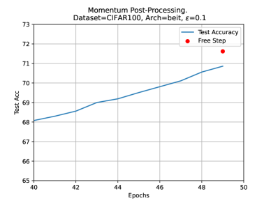
(b) Momentum Post-Processing

Figure 4: Ablation of momentum parameter during training (left) and post processing of the parameter exponential moving average stored in the momentum buffer to take an extra step ’for free’ (right). Use of both methods increases performance slightly.

Momentum Accelerates Convergence.

Despite the exhaustive study of the acceleration of gradient descent with momentum done by prior work (Sutskever et al., 2013; Qian, 1999) work on DP-SGD generally eschews the use of a momentum term. A notable exception (Mehta et al., 2022a) use AdamW rather than SGD with momentum; in a later section we discuss the reason to prefer SGD with momentum. The reason to use momentum to accelerated the convergence of DP-SGD is straightforward: the exponentially moving average of noisy gradients will have higher SNR than individual gradients. Furthermore, momentum is shown to provably benefit normalized SGD (Cutkosky and Mehta, 2020). In Fig. 4 we observe that momentum complements our new linear scaling rule and accelerates convergence. Separately, we report the improvement of taking a step ’for free’ in the direction of the exponential moving average stored during training in the momentum buffer. Note that this exponential moving average is in no way tied to momentum, and it is equivalent to perform DP-SGD without acceleration, store an exponential moving average of gradients with decay parameter $\gamma=0.9$, and then take an additional step in the direction of the stored gradient average after training has finished; we only use the momentum buffer for ease of implementation. As we discuss above when introducing the new linear scaling rule, we maximize performance by maximizing SNR and terminating training while the model is still improving. Intuitively we therefore expect that the momentum buffer will contain a good estimate of the direction of the next step that we would have taken had we continued training, and taking a step in this direction with our usual learning rate should only improve performance without any privacy loss. We use momentum with $\rho=0.9$ in all other experiments and also take a ’free step’ at the end of private training.

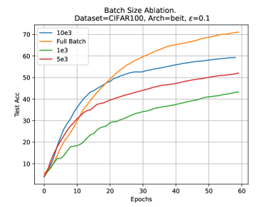
(a) Batch Size

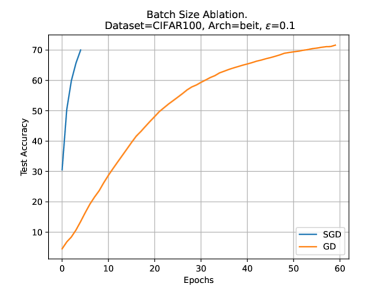
(b) Gradient Descent vs SGD

Figure 5: Ablation of batch size. Left: We vary the batch size using the learning rate and number of iterations tuned for full batch; all other batch sizes perform much worse. Right: We compare SGD and GD. For SGD we tune the batch size jointly with learning rate and number of iterations, arriving at a batch size of 4096 and plot the best performing run against full batch.

Full Batches Optimize Signal-to-Noise Ratio.

Since its inception, the use of privacy amplification via Poisson subsampling and RDP has been a mainstay in the DP community (Zhu and Wang, 2019; Wang et al., 2019; Erlingsson et al., 2018). Prior work almost universally uses privacy amplification via subsampling, but as early as (McMahan et al., 2017), and more recently in (De et al., 2022) it has become apparent that DP-SGD can actually benefit from large batch sizes because the signal-to-noise ratio (SNR) improves. Note that the noise term in 2 is divided by the batch size, so if we are willing to give up amplification via subsampling entirely, we can reduce the noise by a factor of $5e4$ for the benchmark computer vision tasks. In Fig. 5 we report the improvement of full-batch DP-GD over Poisson subsampled DP-SGD. We attribute the success of DP-GD to the improvement in SNR. For example, we achieve 91.52$\%$ accuracy on CIFAR10 for $\varepsilon=0.01$ when training for 100 epochs with learning rate $\eta=0.01$ and noise multiplier $\sigma=2561$. When the noise is divided by the batch size, the effective noise multiplier is $\frac{\sigma}{|B|=5e4}=0.05$ and the SNR is $\frac{1}{0.051}=20$. When we use subsampling with sampling probability $p=0.2$ and train for the same number of epochs under the same privacy budget, our effective noise multiplier is $\frac{\sigma}{|B|}=\frac{1145}{1e4}=0.114$, and the corresponding SNR of ${\frac{1}{0.114}=8.7}$ is much worse than in the full batch setting. Although at first glance our analysis merely supports the typical conclusion that large batches are better in DP-SGD, (De et al., 2022) observe that DP-SGD is still preferrable to DP-GD because minibatching produces the optimal choice of noise multiplier. Our findings run counter to this: as discussed above, we contend that performance depends not only on the optimal noise multiplier but on our new linear scaling rule, and DP-GD unlocks the use of larger step sizes (Goyal et al., 2017). We use DP-GD instead of DP-SGD in all other experiments, removing the batch size from the hyperparameter tuning process and improving the overall privacy cost of deploying our baselines (Papernot and Steinke, 2021).

Small Clipping Norms Bias Optimization.

The standard deviation of the noise added in DP-SGD scales with the sensitivity of the update, defined by the clipping norm parameter. To decrease the amount of noise added, prior work has used very strict clipping (Mehta et al., 2022a; Bu et al., 2022). Intuitively, if the clipping norm parameter is already chosen to be some value smaller than the norm of the unclipped gradient, the gradient estimator is no longer unbiased and this may have a negative impact on optimization. In Fig. 6 we observe that decreasing the clipping norm below 1 only degrades performance. As we can see in equation 2, further decreasing the clipping norm is equivalent to training with a smaller learning rate, and this is suboptimal because Fig. 2 indicates that we can prefer to use larger learning rates. We use a clipping norm of 1 in all other experiments.

Initializing Weights to Zero Mitigates Variance in DP-GD.

(Qiao et al., 2019) propose initializing the model parameters to very small values to improve the stability of micro-batch training, and (De et al., 2022) find that applying this technique to DP-SGD improves performance. In Fig. 6 we ablate the effectiveness of zero initialization with standard He initialization and find that the best performance comes from initializing the weights uniformly to zero. We initialize the classifier weights to zero in all other experiments.

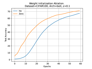
(a) Weight Initialization

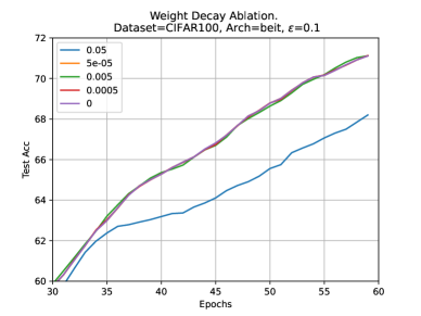
(b) Weight Decay

Figure 6: Ablation of two previously proposed methods: zero initialization of parameters and weight decay. Zero initialization increases accuracy in all experiments, but weight decay only degrades performance.

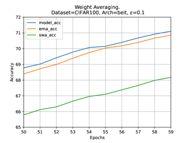
(a) Weight Averaging

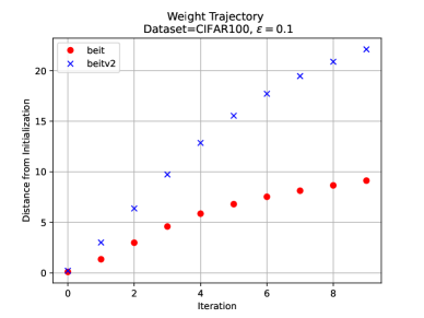
(b) Weight Trajectory

Figure 7: Left:Ablation of Weight Averaging. Right: Plot of distance from initialization. Weight Averaging does not improve performance because the model is monotonically moving away from the initialization and weight averaging cannot ’catch up’.

Weight Averaging Cannot Catch Up To Accelerated Fine-Tuning.

(Shejwalkar et al., 2022) perform an in-depth empirical analysis and find that averaging the intermediate model checkpoints reduces the variance of DP-SGD and improves model performance.  (De et al., 2022) first proposed the use of an Exponential Moving Average (EMA) to mitigate the noise introduced by DP-SGD. Previously, methods that use stochastic weight averaging (SWA) during SGD have been proposed and are even available by default in PyTorch (Izmailov et al., 2018). The idea of averaging weights to increase acceleration was first proposed by (Polyak and Juditsky, 1992), and is theoretically well-founded. In Fig. 7 we compare EMA and SWA with no averaging and find that no averaging performs the best. This is because weight averaging methods work well when optimization has converged and the model is plotting a trajectory that orbits around a local minima in the loss landscape (Izmailov et al., 2018). That is to say, the model’s distance from the initialization does not continually increase and at some point stabilizes so that the weight averaging method can ’catch up’. However, as discussed in Fig. 1 the optimal number of iterations for DP-RAFT is to train for longer epochs without decaying the learning rate for convergence, because when the model converges the SNR decays. This is corroborated by Fig. 7, where we see that the distance from initialization is monotonically increasing. Our findings run counter to those of (Shejwalkar et al., 2022) for hyperparameters in line with our proposed linear scaling rule because we find that the best optimization regime for DP-RAFT is precisely one where weight averaging can never catch up to the optimization trajectory. Therefore, the averaging methods only serve to lag one step behind no averaging.

Data Augmentation Does Not Work When Freezing Embeddings.

Data augmentation is used during training to bias the model towards selecting features that are invariant to the rotations we use in the augmentations.  (Geirhos et al., 2018) find that feature extractors pretrained on ImageNet are naturally biased towards texture features.  (De et al., 2022) eschew traditional data augmentation and instead propose the use of multiple dataset augmentations or "batch augmentation", first introduced by (Hoffer et al., 2019), to mitigate the variance of DP-SGD. In Fig. 8 we ablate the effectiveness of batch augmentation and find that it does not noticeably improve accuracy during transfer learning. This is because dataset augmentation changes the prior of the model when training the entire network (Shorten and Khoshgoftaar, 2019), but when we freeze all layers but the classifier, the model does not have the capacity to change to optimize for the prior introduced by data augmentation, because the embedding layer is frozen.

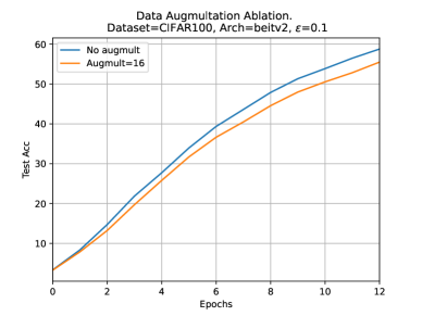
(a) CIFAR100 (hard)

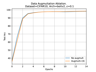
(b) CIFAR10 (easy)

Figure 8: Ablation of Data Augmultation on two datasets. On both datasets, Data Augmultation lags behind the baseline because there is much more training data, and even at the end, Data Augmultation does not have a noticeable improvement.

Weight Decay Is Not Needed When Freezing Embeddings.

Regularization methods such as weight decay are commonly used during pretraining to prevent overfitting, and the feature extractors we use are pretrained with AdamW (Dosovitskiy et al., 2020). One of the benefits of weight decay during fine-tuning is limiting the change of the embedding layer to not overfit and thus retain the features learned during pretraining (Kumar et al., 2022a). In the ongoing debate on whether to use weight decay during fine-tuning (Touvron et al., 2021), we submit that weight decay should not be used in private fine-tuning. In Fig. 6 we ablate a range of values of the weight decay parameter and observe that increasing the weight decay beyond a negligible amount (the gradient norm is $\approx 1e-2$) only decreases accuracy, and no value of the weight decay increases accuracy. There are two reasons for this. The first is that we initialize the weights of the model to zero, so we do not expect the gradients to be large. The second is that we only train the last layer, and therefore there is no need to regularize the training of the embedding layer. This supports the conclusion of (Kumar et al., 2022b) that SGD with momentum is outperforms AdamW as long as the embedding layer is not updated.

Table 5: Finetuning GPT-2 on Persona-Chat dataset including full model and different layers of model. We also include non-private baseline.

DP Guarantee	(Li et al., 2021)	Full Model	Last Block	First-Last-Block
$\varepsilon=0.5$	-	$21.25$	-	-
$\varepsilon=3$	$24.59$	$17.91$	$19.80$	$18.93$
$\varepsilon=8$	$23.57$	$17.27$	$19.20$	$18.26$
$\varepsilon=\infty$	$18.52$	$13.37$	-	-

(a) $\varepsilon=3$

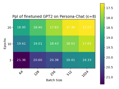
(b) $\varepsilon=8$

Figure 9: Comparison of perplexity at different batch size and epochs of GPT2 on Persona-Chat dataset.

Finetuning Large Language Models.

As shown by (Li et al., 2021; Yu et al., 2021a), privately fine-tuning pretrained language models can achieve performance close to non-private models. Here we focus on Persona-Chat dataset (Zhang et al., 2018b) as there is a relatively large gap between private and non-private models in the reported metric in (Li et al., 2021) (probably because they did not fine-tune for best hyperparameters). Here we do hyperparameter tuning to further decrease the perplexity (See Appendix A for hyper-parameters search range). We report the result in Table 5 and we can see that we can push the perplexity under $18$ for $\varepsilon=3$ and $\varepsilon=8$ and the result for $\varepsilon=0.5$ is better than $\varepsilon=8$ in (Li et al., 2021). Furthermore, we also report the perplexity of GPT2 on the Persona-Chat dataset at different epochs and batch size in Figure 9 (with tuned learning rate in Appendix A) and we can see that larger batch size and longer epochs can achieve better perplexity, which is consistent with (Li et al., 2021) on lager batch size and learning rate are better at fixed training epochs and larger batch size better at fixed updated steps. Besides, we also investigate fine-tuning multiple layers. With letting the embedding layer and last LayerNorm layer in transformer trainable, we consider fine-tuning only last block in transformer, first and last block in transformer and report the result in Table 5 and we can see that the best perplexity is achieved by fine-tuning the whole model.

Appendix A Experimental Set-up for Finetuning for GPT-2

We write code based on winners of ConvAI2 competition and private-transformers library. We first do clipping norm $[0.1,0.2,0.5,1.0]$, learning rate in $[2,5,10,20,50]\times 10^{-5}$, batch size $64$ and epochs $[3,10,20]$ at $\varepsilon=3$ and $\varepsilon=8$ and find that the clipping norm in this range achieves almost same perplexity with other hyperparams fixed. We then do hyperparameter tuning as reported in Table 6 for finetuning GPT2.

Table 6: Set of hyper-parameters used in the finetuning GPT-2.

Parameter	Values
Clipping Norm	$0.1$
Learning Rate	$[2,5,10,20,50,100]\times 10^{-5}$
Batch Size	$[64,128,256,512,1024]$
Epochs	$[3,10,20]$

Appendix B Further Results for Computer Vision Tasks

We provide full heatmaps and pareto frontiers for all datasets and the 3 best performing models (we do not perform a full evaluation on the ViT in order to minimize any knowledge leak for the evaluation of the linear scaling rule with the strategy in  [Mehta et al., 2022a]). We note that while all of these datasets are arguably in-distribution, our focus is on comparing the regime of optimization preferred by DP-RAFT to those of other works, and this is achieved by producing results on benchmark tasks. We further note that STL10 is explicitly in-distribution for the pretraining dataset (ImageNet); we only use this dataset as a temporary stand-in for evaluation on ImageNet-1k, a common benchmark in prior work [Mehta et al., 2022a] to minimize the computational burden.

Hyperparameter Tuning and Selecting Epsilon.

Prior work often uses unrealistic values of $\varepsilon$ that provide no real privacy guarantee. While some prior work makes the case that hyperparameters need to be tuned even for non-private learning and can be chosen beforehand, we show that this is not the case. Not only are the optimal choices of key hyperparameters different between training from scratch and transfer learning [Li et al., 2020], they are also different for non-private and private transfer learning [Li et al., 2021, De et al., 2022]. We now provide guidelines for selecting $\varepsilon$ and broad intuition behind our choice to design a system that minimizes dependence on hyperparameters.

For a decade the standard values of $\varepsilon$ proposed for privacy preserving statistics queries have fallen in the range of $0.1$ in line with $e^{\varepsilon}\approx 1+\varepsilon$ for $\varepsilon\ll 1$ [Dwork et al., 2006], and recently surveyed DP deployments generally abide by the rule of selecting $\varepsilon\approx 0.1$ [Dwork et al., 2019]. We know that while all small values of $\varepsilon$ generally behave the same, every large value of $\varepsilon$ is fundamentally different in a unique way [Dwork et al., 2019]. In line with these guidelines, we only evaluate $\varepsilon\in[0.01,1.0]$ and perform most of our ablations on the most challenging task where we can see a range of performance: CIFAR100 for $\varepsilon=0.1$.

(a) CIFAR10 Beitv2

(b) CIFAR10 Beit

(c) CIFAR10 Convnext

(d) CIFAR100 Beitv2

(e) CIFAR100 Beit

(f) CIFAR100 Convnext

Figure 10: Heatmaps for the reported datasets and architectures; lighter is better. Note that the scale of the axes differs from the heatmaps in the main body; this will be fixed in a future update. $\varepsilon$ increases left to right with a different value for each heatmap according to: $[0.01,0.05,0.1,0.2,0.3,0.4,0.5,0.6,0.7,0.8,0.9,1.0]$, epochs increase from left to right on the x-axis of each heatmap according to: $[1,5,10,20,30,40,50,60,70,80,90,100]$, and the learning increases from top to bottom on the y-axis of each heatmap according to: $[0.01,0.05,0.1,0.15,0.2,0.25,0.5,1.0]$. As $\varepsilon$ increases, left to right, the optimal hyperparameters trend towards longer training with lower learning rates (bottom right).

(a) STL10 Beitv2

(b) STL10 Beit

(c) STL10 Convnext

(d) FashionMNIST Beitv2

(e) FashionMNIST Beit

(f) FashionMNIST Convnext

Figure 11: Heatmaps for the reported datasets and architectures; lighter is better. Note that the scale of the axes differs from the heatmaps in the main body; this will be fixed in a future update. $\varepsilon$ increases left to right with a different value for each heatmap according to: $[0.01,0.05,0.1,0.2,0.3,0.4,0.5,0.6,0.7,0.8,0.9,1.0]$, epochs increase from left to right on the x-axis of each heatmap according to: $[1,5,10,20,30,40,50,60,70,80,90,100]$, and the learning increases from top to bottom on the y-axis of each heatmap according to: $[0.01,0.05,0.1,0.15,0.2,0.25,0.5,1.0]$. As $\varepsilon$ increases, left to right, the optimal hyperparameters trend towards longer training with lower learning rates (bottom right).

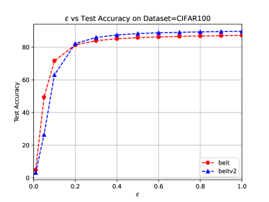
(a) CIFAR100 Test Accuracy

(b) CIFAR100 Total Step Size

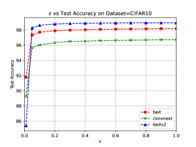
(c) CIFAR10 Test Accuracy

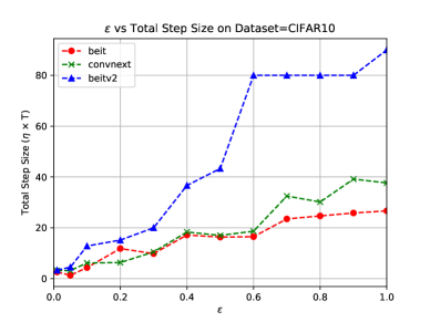
(d) CIFAR10 Total Step Size

Figure 12: Pareto frontier for $\varepsilon$ vs test accuracy and total step size for CIFAR10, and CIFAR100. Beitv2 excels for larger values of $\varepsilon$ but beit and convnext are better for smaller values of $\varepsilon$. The inflection point varies across datasets.

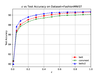
(a) FashionMNIST Test Accuracy

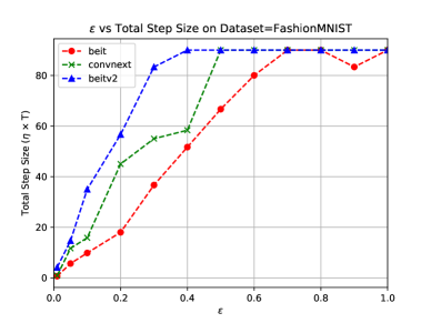
(b) FashionMNIST Total Step Size

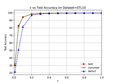
(c) STL10 Test Accuracy

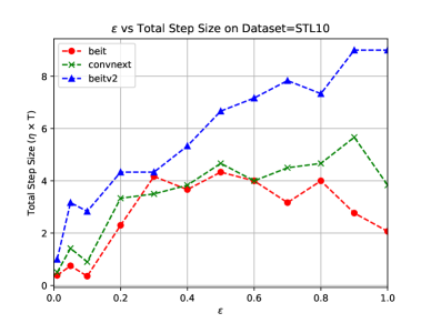
(d) STL10 Total Step Size

Figure 13: Pareto frontier for $\varepsilon$ vs test accuracy and total step size for STL10 and FashionMNIST. Beitv2 excels for larger values of $\varepsilon$ but beit and convnext are better for smaller values of $\varepsilon$. The inflection point varies across datasets.