On inclusion of time-varying source in the acoustic wave equation

Abstract

Acoustic wave equation is a partial differential equation (PDE) which describes propagation of acoustic waves through a material. In general, the solution to this PDE is nonunique. Therefore, it is necessary to impose initial conditions in the form of Cauchy conditions for obtaining a unique solution. Theoretically, solving the wave equation is equivalent to representing the wavefield in terms of a radiation source which possesses finite energy over space and time. The radiation source is represented by a forcing term in the right-hand-side of the wave equation. In practice, the source may be represented in terms of normal derivative of pressure or normal velocity over a surface. The pressure wavefield is then calculated by solving an associated boundary value problem via imposing conditions on the boundary of a chosen solution space. From an analytic point of view, this manuscript aims to review typical approaches for obtaining unique solution to the acoustic wave equation in terms of either a volumetric radiation source $s$, or a surface source in terms of normal derivative of pressure $(\partial/\partial\bm{n})p$ or normal velocity $u^{\bm{n}}=\bm{u}\cdot\bm{n}$, where $\bm{n}$ is a unit vector normal to the surface. A numerical approximation of the derived formulae will then be explained. The key step for numerically approximating the derived analytic formulae is inclusion of source, and will be studied carefully in this manuscript.

1. Introduction

Acoustic wave equation is one of the most important partial differential equations (PDEs) in mechanics [1, 2, 3, 4, 5, 6], and has broad ranges of applications [7, 8, 9, 10, 11, 12, 13, 14, 15, 16, 17, 18]. The forcing term in the right-hand-side of this second-order PDE can be assumed time instant or time-varying. For biomedical applications, one important example for formation of time-instant acoustic sources is photo-acoustic (PA) effect, the process of absorption of optical energy, its conversion to heat and generation of local acoustic pressures via therm-elastic expansion. Because the PA effect, which leads to local rises in pressure, occurs in a time few orders of magnitude shorter than the time for propagation of acoustic waves, the acoustic source is assumed time-instant [19, 20, 21, 22, 23, 24, 25, 26, 27, 28, 29, 30, 31, 32, 33, 34, 35, 36, 37]. For time-varying sources, also known as radiation sources, an important example is radiation from vibrating sources, e.g., piezolectric transducers [38]. Modelling time-varying sources has received growing attention for biomedical applications, for example for full-wave inversion approaches which are used for the purpose of quantitative ultrasound tomography [38, 39, 40, 41, 42, 43, 44, 45, 46, 47, 48, 49, 50, 51, 52, 53, 54], or for treatment planning using focused ultrasound, which is an emerging technology for treatment of medical disorders via targeting deep tissues by ultrasonic energy [55, 56, 57, 58, 59, 60, 61]. For the latter, an accurate solution to the wave equation is very important because of safety reasons [62].

The solution to the wave equation is typically nonunique. Therefore, Cauchy initial conditions in terms of the wavefield and its time derivative at time origin are enforced for obtaining unique solution. These initial conditions establish a causal relation between solution wavefield and source, i.e., the solution wavefield vanishes prior to the time the source starts radiating. Therefore, solving the wave equation can be expressed as uniquely representing the propagated wavefield in terms of the radiation source (forcing term) via applying the causality conditions. The radiation source $s$ is defined over a finite volume and time and is assumed to possess finite energy, i.e., it is square-integrable over space and time. Furthermore, the source may be defined as a surface source in terms of normal derivative of pressure $(\partial/\partial\bm{n})p$ or normal velocity $u^{\bm{n}}=\bm{u}\cdot\bm{n}$, where $\bm{n}$ is a unit vector normal to the surface. To obtain a unique solution for a surface source, in addition to assumption of causality conditions, conditions must be imposed on the boundary of a chosen solution space. The choice for the solution space and the conditions applied on its boundary are dependent on geometry of the problem and the source.

It will be shown that a numerical approximation of the wave equation is equivalent to representing the propagated wavefield as a weighted superposition of actions of a causal Green’s function on the source defined on a distribution of sampled point sources over a finite volume or surface and over finite time of radiation of source. The weighting parameter for each sampled point is the contribution of the volume or surface of the source to that sampled point. The derived formulae for a numerical approximation of the wave equation will be compared with a state-of-the-art numerical approach [3]. The key step for an accurate numerical approximation of the wave equation in the time domain was found to be modelling the mass source, specifically how to model the mass source such that it is included in the associated numerical systems correctly and with consistent units.

Section 2 introduces the wave equation in the time domain. This section will explain how a unique solution to the wave equation can be obtained using homogeneous Cauchy conditions, which establish a causal relation between solution wavefield and radiation source. A primary solution to the wave equation, which describes the propagated wavefield in terms of a volumetric radiation source, will be described, and a Kirchhoff-Helmholtz solution to the wave equation, which solves the wavefield in terms of a surface source, will be derived. It will be explained how the boundary conditions of Dirichlet, Neumann or Mixed types can be imposed for obtaining a unique solution for an arising over-determined formula describing the Kirchhoff-Helmholtz solution. Section 3 describes the primary and Kirchhoff-Helmholtz solutions to the wave equation in the frequency domain. Furthermore, a Rayleigh-sommerfeld solution to the wave equation will be explained for cases in which the surface source is defined over a flat plane. Section 4 describes how the derived time-domain analytical formulae can be numerically approximated on a grid discretised in space and time. Specifically, this section describes how the mass source is modelled and is given as an input to numerical systems for solving the wave equation in the time domain without the need for changing units of quantities in the wave equation, as done in [5], section 2.4., equations (2.18) and (2.19). It will be shown that a numerical solution to the wave equation is equivalent to computing a weighted superposition of actions of a causal Green’s function on a distribution of point sources over a finite volume or surface and over finite time of radiation of source. In section 5, the derived analytic formulae in the time domain will be compared to their numerical approximation on a discretised grid for a source defined on a single point in space. It will be shown that the action of the Green’s function on this point source gives nonphysical quantities, but computing a weighted superposition of these actions on a distribution of point sources over a volume or surface of support of the source will give the wavefield representing the solution to the wave equation in time. Section 6 contains a brief discussion about the explained approaches and the obtained numerical results.

2. Wave equation in the time domain

This section considers the propagation of acoustic waves from a real-valued space and time-varying source in an infinite, isotropic and homogeneous medium in free space. Let $\bm{x}=(x^{1},...,x^{d})$ denote a spatial position in $\mathbb{R}^{d}$ with $d\in\{2,3\}$ the number of dimensions. (Here, the analysis is done for $d=3$, but it also holds for $d=2$ by changing the volumes to planes, and planes to lines. A line source produces acoustic waves which propagate as cylindrical waves in a 3D medium, and is equivalent to an omnidirectional point source in a 2D medium.) The real-valued wavefield satisfies the inhomogeneous wave equation, which is in the form

$$\frac{1}{c^{2}}\frac{\partial^{2}}{\partial t^{2}}p(\bm{x},t)-\rho_{0}\nabla\cdot\Big{[}\frac{1}{\rho_{0}}\nabla p(\bm{x},t)\Big{]}=s(\bm{x},t).$$ (1)

Here, the term in the right-hand-side is the forcing term $s(\bm{x},t)$, also known as radiation source, and is assumed compactly supported in $\chi_{s}=\{\bm{x}\in\nu_{s},\ t\in[0,T_{s}]\}$, where $\nu_{s}$ is a spatial volume, and $[0,T_{s}]$ is radiation time of the source. The source has units $\text{kgm}^{-\text{d}}\text{s}^{-2}$. It is assumed that the source $s$ is square-integrable in $\chi_{s}$. In addition, $c$ is velocity of wave propagation in medium and has units $\text{ms}^{-1}$. Also, $\rho_{0}$ is ambient density of medium, and has units $\text{kgm}^{-\text{d}}$. Furthermore, $p$ denotes the pressure wavefield, which is the unknown parameter of the wave equation, and has units $\text{kgm}^{2-\text{d}}\text{s}^{-2}$ (or Pascal). By assuming constant values for $\rho_{0}$, the wave equation (1) is reduced to its canonical form

$$\Big{[}\frac{1}{c^{2}}\frac{\partial^{2}}{\partial t^{2}}-\nabla^{2}\Big{]}p(\bm{x},t)=s(\bm{x},t).$$ (2)

2.1. Cauchy conditions for unique solution.

The solution to the wave equation is nonunique. A unique solution is obtained by confining the wavefield to a particular solution which is causally related to the source, i.e., a wavefield $p$ which vanishes prior to the time $t=0$, the initial time of source radiation. By imposing the Cauchy conditions

$$p_{+}(\bm{x},t)|_{t=0}=0,\ \ \ \frac{\partial}{\partial t}p_{+}(\bm{x},t)|_{t=0}=0,$$ (3)

a causal solution to the wave equation (2) is obtained, where the subscript $+$ stands for the causality. The problem of solving the inhomogeneous wave equation (2), together with the causality conditions, i.e., Cauchy conditions (3), is called radiation problem. Note that by setting the forcing term $s$ zero, and relaxing the Cauchy conditions (3) to arbitrary and inhomogeneous fields at $t=0$, the wave equation (2) will be an initial-value problem, which arises for example in photoacoustic tomography. The focus of this manuscript is on analytic and numerical solutions to the radiation problem.

2.2. Green’s function solution.

Consider the wave equation (2) as a radiation problem for a particular choice $s(\bm{x},t)=\delta(\bm{x}-\bm{x}^{\prime})\delta(t-t^{\prime})$, where $\delta(\cdot)$ is the Dirac delta function. In an infinite free space, a Green’s function solution to the wave equation then satisfies

$$\Big{[}\frac{1}{c^{2}}\frac{\partial^{2}}{\partial t^{2}}-\nabla^{2}\Big{]}g(\bm{x}-\bm{x}^{\prime},t-t^{\prime})=\delta(\bm{x}-\bm{x}^{\prime})\delta(t-t^{\prime}),$$ (4)

where $\bm{x}$ and $t$ are general parameters of the wave equation, and $\bm{x}^{\prime}$ and $t^{\prime}$ are the fixed parameters, which can be chosen any values in space and time. For brevity, the Green’s function will be written in the form

$$g(\bm{x}_{d},t_{d})=g(\bm{x}-\bm{x}^{\prime},t-t^{\prime}),$$ (5)

where $\bm{x}_{d}=\bm{x}-\bm{x}^{\prime}$ and $t_{d}=t-t^{\prime}$. Similar to the wave equation (2), a unique solution to Eq. (4) is satisfied by assuming a causality condition for the Green’s function, i.e., $g_{+}(\bm{x}_{d},t_{d})=0$ for $t_{d}<0$. By applying causality condition, the wave equations (2) and (4) will be in the forms

$$\Big{[}\frac{1}{c^{2}}\frac{\partial^{2}}{\partial t^{\prime 2}}-\nabla_{\bm{x}^{\prime}}^{2}\Big{]}p_{+}(\bm{x}^{\prime},t^{\prime})=s(\bm{x}^{\prime},t^{\prime}),$$ (6)

and

$$\Big{[}\frac{1}{c^{2}}\frac{\partial^{2}}{\partial{t^{\prime}}^{2}}-\nabla_{\bm{x}^{\prime}}^{2}\Big{]}g_{+}(\bm{x}-\bm{x}^{\prime},t-t^{\prime})=\delta(\bm{x}-\bm{x}^{\prime})\delta(t-t^{\prime}),$$ (7)

where $\bm{x}$ and $t$ are now the fixed parameters, whose values are confined to a closed set $\chi=\{\bm{x}\in\nu,t\in[t_{0},t_{1}]\}$ of free space and time within which the solution is sought [63]. Now, multiplying (6) by $g_{+}(\bm{x}-\bm{x}^{\prime},t-t^{\prime})$ and (7) by $p_{+}(\bm{x}^{\prime},t^{\prime})$, and then subtracting the modified (7) from the modified (6), yield

$$(\nabla^{2}g_{+})p_{+}-g_{+}\nabla^{2}p_{+}-\frac{1}{c^{2}}\Big{[}(\frac{\partial^{2}}{\partial{t^{\prime}}^{2}}g_{+})p_{+}-g_{+}\frac{\partial^{2}}{\partial{t^{\prime}}^{2}}p_{+}\Big{]}=g_{+}s-\delta(\bm{x}_{d})\delta(t_{d})\ p_{+},$$ (8)

where the dependence on space and time has been neglected for brevity. Now, integrating the left side of Eq. (8) over the chosen spatio-temporal solution set $\chi$ gives

$$\int_{t_{0}}^{t_{1}}dt^{\prime}\ \int_{\nu}d\bm{x}^{\prime}\ \nabla\cdot\Big{[}(\nabla g_{+})p_{+}-g_{+}\nabla p_{+}\Big{]}-\frac{1}{c^{2}}\int_{t_{0}}^{t_{1}}dt^{\prime}\ \int_{\nu}d\bm{x}^{\prime}\ \frac{\partial}{\partial t^{\prime}}\Big{[}(\frac{\partial}{\partial t^{\prime}}g_{+})p_{+}-g_{+}\frac{\partial}{\partial t^{\prime}}p_{+}\Big{]}.$$ (9)

Now, applying the well-known Green’s theorem to the first term in (9), taking the temporal integral of the second term in (9), and then taking the integral of the right-hand side in (8) over the solution set $\chi$, give [63]

$$\begin{split}&\int_{t_{0}}^{t_{1}}dt^{\prime}\ \int_{\partial\nu}dS^{\prime}\ \Big{[}(\frac{\partial}{\partial\bm{n}^{\prime}}g_{+})p_{+}-g_{+}\frac{\partial}{\partial\bm{n}^{\prime}}p_{+}\Big{]}-\frac{1}{c^{2}}\ \int_{\nu}d\bm{x}^{\prime}\ \Big{[}(\frac{\partial}{\partial t^{\prime}}g_{+})p_{+}-g_{+}\frac{\partial}{\partial t^{\prime}}p_{+}\Big{]}\Big{|}_{t_{0}}^{t_{1}}=\\ &\int_{t_{0}}^{t_{1}}dt^{\prime}\ \int_{\nu}d\bm{x}^{\prime}\ g_{+}s\ -\begin{cases}p_{+},&\text{if}\ \bm{x}\in\nu,t\in[t_{0},t_{1}]\\ 0,&\text{otherwise},\end{cases}\end{split}$$ (10)

where $\bm{n}^{\prime}$ is an outward unit vector normal to the surface $\partial\nu$.

2.2.1. Primary solution

A primary solution for all space and all time can be obtained by enlarging the spatio-temporal set $\chi$ to infinity. Accordingly, we take the limits $\nu\rightarrow\infty$, $t_{0}\to-\infty$ and $t_{1}\to\infty$. Now, for the second term in the left-hand-side of Eq. (10), by the assumption of causality, $p_{+}$ vanishes at $t=-\infty$ and $g$ vanishes for the time $t=+\infty$, and the second term will thus drop. In addition, considering that a causal Green’s function gives $g(\bm{x}_{d},t_{d})=0$ unless $x_{d}=ct_{d}$ with $x_{d}=|\bm{x}_{d}|$, the contribution from surface $\partial\nu$ with infinite radius vanishes for any finite and arbitrarily large value for $t_{1}$. Therefore, the left-hand-side of Eq. (10) vanishes as well, and therefore, the primary solution for $p_{+}$ at any pair of $\bm{x}$ and $t$ which lie in the set $\chi$ satisfies

$$p_{+}(\bm{x},t)=\int_{0}^{T_{s}}dt^{\prime}\int_{\nu_{s}}d\bm{x}^{\prime}\ g_{+}(\bm{x}_{d},t_{d})s(\bm{x}^{\prime},t^{\prime}).$$ (11)

Considering the infinity assumptions used for the set $\chi$, this solution holds over all space and all time. The Primary formula (11) represents the solution wave field in terms of the radiation source $s$, the forcing term in the right-hand-side of the wave equation.

2.2.2. Kirchhoff-Helmholtz solution

The Equation (11), which gives a primary solution, directly maps the forcing term $s$ to the wavefield solution $p_{+}$, and is based on an integration of source $s$ over its volumetric support. However, for many problems, the source is quantified over an external surface. Correspondingly, a more practical formula can be derived based on assuming $\nu$ a finite volume which contains the source volume $\nu_{s}$. It is assumed that the volume $\nu$ has a closed boundary $\partial\nu$, and the space in which the solution is sought is now confined to the volume lying outside $\partial\nu$ [63]. Now, by assuming a causal solution to the wave equation (6) over a time $[t_{0},t_{1}]$ with $t_{0}\to-\infty$ and $t_{1}\to+\infty$ and using an assumption of causality for the Green’s function solution in (7), a solution is sought in the volume $\nu^{\mathcal{C}}$, which is bounded by the closed surface $\partial\nu$ and the closed boundary of a sphere with a radius of infinity. The procedure is the same as in section 2.2.1, except the integral in Eq. (10) is taken over $\nu^{\mathcal{C}}$, instead of $\nu$. Accordingly, the second term in the left-hand-side of Eq. (10) vanishes because of causality of $p_{+}$ and $g$, the same as in section 2.2.1. For the first term in Eq. (10), the contribution of the surface with infinity radius (10) vanishes, as discussed in section 2.2.1. Therefore, the field $p_{+}$ which resides in the solution space $\nu^{\mathcal{C}}$, satisfies [63]

$$\int_{-\infty}^{\infty}dt^{\prime}\ \int_{\partial\nu}dS^{\prime}\ \Big{[}g_{+}\frac{\partial}{\partial\bm{n}^{\prime}}p_{+}-(\frac{\partial}{\partial\bm{n}^{\prime}}g_{+})p_{+}\Big{]}=\begin{split}\begin{cases}p_{+}(\bm{x},t),\ \ \ &\bm{x}\in\nu^{\mathcal{C}}\\ 0,\ \ \ &\bm{x}\in\nu\end{cases}\end{split}$$ (12)

where $\bm{n}^{\prime}$ is a unit vector normal to the surface $\partial\nu$ and directed outward from the interior volume $\nu$ to the exterior volume $\nu^{\mathcal{C}}$ in which the solution is sought. In Eq. (12), the formula for the exterior volume is called first Helmholtz identity, and describes a solution wavefield outside an arbitrary surface $\partial\nu$ bounding the source volume $\nu_{s}$ as a function of the field and its outward-directed normal derivative over that surface. The formula for the internal volume is called second Helmholtz identity, and is a homogeneous integral equation, which establishes a dependence between the field and its normal derivative over the surface $\partial\nu$. Sadly, because of the dependence established by the second Helmholtz identity over the surface $\partial\nu$, the first Helmholtz identity is an over-determined problem. Therefore, boundary conditions must be imposed to make this formula well-posed. A well-posedness requires that the integrand in the Kirchhoff-Helmholtz formula (12) be a function of only the wavefield, only its normal derivative, or a linear combination of both. These can be satisfied by imposing Neumann, Dirichlet or Mixed boundary conditions, respectively. Correspondingly, by imposing homogeneous Dirichlet or Neumann conditions on the boundary surface $\partial\nu$, the formula (12) is reduced to the well-posed formula

$$p_{+}^{D}(\bm{x},t)=-\int_{-\infty}^{\infty}dt^{\prime}\ \int_{\partial\nu}dS^{\prime}\ \Big{(}\frac{\partial}{\partial\bm{n}^{\prime}}g_{+}^{D}(\bm{x}_{d},t_{d})\Big{)}p_{+}(\bm{x}^{\prime},t^{\prime}),\ \ \ g_{+}^{D}(\bm{x}_{d},t_{d})|_{\bm{x}^{\prime}\in\partial\nu}=0,$$ (13)

$$p_{+}^{N}(\bm{x},t)=\int_{-\infty}^{\infty}dt^{\prime}\ \int_{\partial\nu}dS^{\prime}\ g_{+}^{N}(\bm{x}_{d},t_{d})\frac{\partial}{\partial\bm{n}^{\prime}}p_{+}(\bm{x}^{\prime},t^{\prime}),\ \ \ \frac{\partial}{\partial\bm{n}^{\prime}}g_{+}^{N}(\bm{x}_{d},t_{d})|_{\bm{x}^{\prime}\in\partial\nu}=0,$$ (14)

where $\bm{x}\in\nu^{\mathcal{C}}$, and $g_{+}^{D}$ and $g_{+}^{N}$ denote Green’s functions satisfying homogeneous Dirichlet and Neumann conditions on the boundary surface $\partial\nu$, respectively. Note that the formulae (13) and (14) are equivalent by an integration by parts.

3. Wave equation in the frequency domain

In this section, the wave equation is treated in the temporal frequency domain. Here, the temporal Fourier transform of a function or field and its inverse is defined by

$$F(\bm{x},\omega)=\int_{-\infty}^{\infty}dt\ f(\bm{x},t)e^{{i\mkern 1.0mu}\omega t},\ \ \ f(\bm{x},t)=\frac{1}{2\pi}\int_{-\infty}^{\infty}d\omega F(\bm{x},\omega)e^{-{i\mkern 1.0mu}\omega t}.$$ (15)

Taking a temporal Fourier transform of (4) gives the Helmholtz equation of the form

$$\big{[}\frac{\omega^{2}}{c^{2}}+\nabla^{2}\big{]}G(\bm{x}_{d},\omega)=-\delta(\bm{x}_{d}),$$ (16)

where $G(\bm{x}_{d},\omega)$ is the frequency-domain Green’s function, which relates to the time-domain Greens’s function through the pair of equations

$$G(\bm{x}_{d},\omega)=\int_{-\infty}^{+\infty}dt_{d}\ g(\bm{x}_{d},t_{d})e^{{i\mkern 1.0mu}\omega t_{d}},\ \ \ g(\bm{x}_{d},t_{d})=\frac{1}{2\pi}\int_{-\infty}^{+\infty}d\omega\ G(\bm{x}_{d},\omega)e^{-{i\mkern 1.0mu}\omega t_{d}}.$$ (17)

3.1. Causality condition and outgoing Green’s function.

Like Eq. (4), the solution to the inhomogeneous wave equation (16) is not unique, and therefore, constraints must be enforced to obtain a unique solution. It will be shown below that causality condition described for the time-domain wave equation results in a boundary condition at infinity in the temporal frequency domain. The associated Green’s function can be derived by taking a spatial Fourier transform of the Helmholtz equation (16). This approach yields

$$G_{+}(\bm{x}_{d},\omega)=\frac{1}{4\pi}\frac{e^{{i\mkern 1.0mu}kx_{d}}}{x_{d}},$$ (22)

where $x_{d}=|\bm{x}_{d}|$ and $k=\omega/c$ is the wavenumber. Here, the subscript $+$ indicates that the Green’s function is outgoing. Substituting (22) into the inverse Fourier formula defined in the right equation in (17) gives

$$g_{+}(\bm{x}_{d},t_{d})=\frac{1}{2\pi}\int_{-\infty}^{\infty}dk\ \frac{1}{4\pi}\frac{e^{{i\mkern 1.0mu}k(x_{d}-ct_{d})}}{x_{d}}.$$ (23)

Here, the Green’s function is expressed as a superposition of time-harmonic waves with spherical surfaces of constant phase $x_{d}-ct_{d}$. These constant-phase surfaces are outgoing, because by initialising at $t_{d}=0$ and increasing $t_{d}$, a constant phase requires that $x_{d}$ increases proportionally (causality requirement).

Remark 1.

An equivalent causal Green’s function can be obtained for 2D media, where $\bm{x}$ is now a position in a plane. Accordingly, an asymptotic expansion of the 2D Green’s function in a homogeneous medium satisfies

$$G_{+}^{2D}(\bm{x}_{d},\omega)=\frac{{i\mkern 1.0mu}}{4}H_{0}^{+}(kx_{d})\approx\Big{[}\frac{1}{8\pi kx_{d}}\Big{]}^{1/2}e^{{i\mkern 1.0mu}(kx_{d}+\frac{\pi}{4})},\ \ \ kx_{d}\to\infty,$$ (24)

where $kx_{d}$ is the accumulated phase.

3.2. Green’s function solution

This section describes the solutions to the wave equation in the frequency domain. Like section 2.2, the wavefield solution will first be derived in terms of a volumetric radiation source $s$. The taken approach will then be extended to solve the wavefield in terms of a source defined over an external surface of a volumetric space which is the support of the radiation source $s$.

3.2.1. Frequency-domain Primary solution

Below, a primary solution to the inhomogeneous wave equation in the frequency domain is described. Plugging the right equation in (17) into the time-domain primary solution (11), and then applying the replacement

$$S(\bm{x}^{\prime},\omega)=\int_{0}^{T_{s}}dt^{\prime}\ e^{{i\mkern 1.0mu}\omega t^{\prime}}s(\bm{x}^{\prime},t^{\prime}),$$ (25)

yield a frequency-domain primary solution, which is in the form

$$P_{+}(\bm{x},\omega)=\int_{\nu_{s}}d\bm{x}^{\prime}\ G_{+}(\bm{x}_{d},\omega)S(\bm{x}^{\prime},\omega),$$ (26)

where $t_{d}=t-t^{\prime}$ has been used.

Sommerfeld radiation condition. At large distances from the source, an approximate Green’s function can be obtained using a far-field approximation

$$x_{d}=|\bm{x}-\bm{x}^{\prime}|=(x^{2}+{x^{\prime}}^{2}-2\bm{x}\cdot\bm{x}^{\prime})^{1/2}\approx x-\hat{\bm{x}}\cdot\bm{x}^{\prime},\ \ \ x\rightarrow\infty$$ (27)

where $\hat{\bm{x}}=\bm{x}/x$ is a unit vector along $\bm{x}$. Plugging the approximation (27) into the outgoing Green’s function (22), and substituting the resulting far-field approximated Green’s function into Eq. (26), give the Sommerfeld radiation condition (SRC) [63]

$$p_{+}(\bm{x},\omega)\approx f(\hat{\bm{x}},\omega)\frac{e^{{i\mkern 1.0mu}kx}}{x},\ \ \ x\to\infty,$$ (28)

where

$$f(\hat{\bm{x}},\omega)=\frac{1}{4\pi}\int_{\nu_{s}}d\bm{x}\ S(\bm{x},\omega)e^{-{i\mkern 1.0mu}k\hat{\bm{x}}\cdot\bm{x}}.$$ (29)

Alternatively, the SRC can be expressed using

$$\lim_{x\to\infty}x^{\frac{d-1}{2}}\Big{[}\frac{\partial}{\partial x}P_{+}(\bm{x},\omega)-{i\mkern 1.0mu}kP_{+}(\bm{x},\omega)\Big{]}\to 0,$$ (30)

where we remind that $d\in\{2,3\}$ stands for the number of dimensions. Eq. (30) can be derived directly from (28).

3.2.2. Frequency-domain Kirchhoff-Helmholtz solution

The frequency-domain version of the Kirchhoff-Helmholtz formula (12) gives [63]

$$\int_{\partial\nu}dS^{\prime}\ \Big{[}G_{+}(\bm{x}_{d},\omega)\frac{\partial}{\partial\bm{n}^{\prime}}P_{+}(\bm{x}^{\prime},\omega)-\big{(}\frac{\partial}{\partial\bm{n}^{\prime}}G_{+}(\bm{x}_{d},\omega)\big{)}P_{+}(\bm{x}^{\prime},\omega)\Big{]}=\begin{split}\begin{cases}P_{+}(\bm{x},\omega),\ \ \ &\bm{x}\in\nu^{\mathcal{C}}\\ 0,\ \ \ &\bm{x}\in\nu,\end{cases}\end{split}$$ (31)

where it is reminded that $\bm{n}^{\prime}$ is a unit vector and outwardly normal from the interior volume $\nu$, which is the support of the source volume $\nu_{s}$, to the exterior solution space $\nu^{\mathcal{C}}$. As discussed in section 2.2.2, the equation for $\bm{x}\in\nu^{\mathcal{C}}$ is termed the first Helmholtz identity, and is an over-determined problem. The reason is that because for $\bm{x}\in\nu$, known as the second Helmholtz identity, the surface integral vanishes, a dependence is established between the field and its normal derivative over $\partial\nu$. Therefore, conditions must be imposed on the surface $\partial\nu$ to make the problem well-posed. Correspondingly, by imposing the Dirichlet or Neumann boundary conditions, the formula (31) is reduced to

$$P_{+}^{D}(\bm{x},\omega)=-\int_{\partial\nu}dS^{\prime}\ \Big{(}\frac{\partial}{\partial\bm{n}^{\prime}}G_{+}^{D}(\bm{x}_{d},\omega)\Big{)}P_{+}(\bm{x}^{\prime},\omega),\ \ \ G_{+}^{D}(\bm{x}_{d},\omega)|_{\bm{x}^{\prime}\in\partial\nu}=0,$$ (32)

$$P_{+}^{N}(\bm{x},\omega)=\int_{\partial\nu}dS^{\prime}\ G_{+}^{N}(\bm{x}_{d},\omega)\frac{\partial}{\partial\bm{n}^{\prime}}P_{+}(\bm{x}^{\prime},\omega),\ \ \ \frac{\partial}{\partial\bm{n}^{\prime}}G_{+}^{N}(\bm{x}_{d},\omega)|_{\bm{x}^{\prime}\in\partial\nu}=0,$$ (33)

where $\bm{x}\in\nu^{\mathcal{C}}$, and $G^{D}$ and $G^{N}$ are the Green’s functions satisfying the homogeneous Dirichlet and Neumann boundary conditions over $\partial\nu$, respectively. The formulae (32) and (33) are equivalent by an integration by parts.

3.2.3. Rayleigh-Sommerfeld solution

A common Green’s approach for solving the boundary-value problem of the Helmholtz wave equation is the Rayleigh-Sommerfeld solution. Using this approach, the solution space $\nu^{\mathcal{C}}$ is taken a half-space which is bounded by a plane $\partial\nu$ and an infinite hemisphere. For simplicity, the bounding plane is assumed $x^{3}=0$, and the solution is sought in the half-space $x^{3}>0$. As discussed above, the associated Kirchhoff-Helmholtz formula is over-determined. To make this problem well-posed, the boundary conditions of the form Dirichlet or Neumann are imposed on $\partial\nu$, and the SRC condition is applied on the infinite surface. A popular method for solving this boundary-value problem is method of images [63]. Accordingly, $\bm{x}$ and $\bm{x}^{\prime}$ are used to denote the position of the general field and a point source in a 3D medium, and it is assumed that both lie in the half-space $\nu^{\mathcal{C}}=\{\bm{x}:x^{3}>0\}$. Using the notation $\bm{x}^{\prime}=(x^{\prime 1},x^{\prime 2},x^{\prime 3})$, another image point $\tilde{\bm{x}}^{\prime}=(x^{\prime 1},x^{\prime 2},-x^{\prime 3})$ is introduced [63]. Accordingly, considering that $\bm{x}$ and $\tilde{\bm{x}}^{\prime}$ lie at different sides of the plane, and therefore $\delta(\bm{x}-\tilde{\bm{x}}^{\prime})=0$, a Helmholtz equation with an augmented forcing term can be defined in the form

$$\big{[}k^{2}+\nabla_{\bm{x}}^{2}\big{]}G_{+}^{N}(\bm{x}-\bm{x}^{\prime},\omega)=-\delta(\bm{x}-\bm{x}^{\prime})-\delta(\bm{x}-\tilde{\bm{x}}^{\prime}),$$ (34)

where the Green’s function $G_{+}^{N}$ satisfies

$$G_{+}^{N}(\bm{x}_{d},\omega)=G_{+}(\bm{x}-\bm{x}^{\prime},\omega)+G_{+}(\bm{x}-\tilde{\bm{x}}^{\prime},\omega),$$ (35)

and also satisfies the SRC condition over the infinite surface. For a point source $\bm{x}^{\prime}$ which lies on the bounding plane $x^{3}=0$, $|\bm{x}-\tilde{\bm{x}}^{\prime}|=|\bm{x}-\bm{x}^{\prime}|$, and thus the Green’s function in (35) satisfies

$$G_{+}^{N}(\bm{x}_{d},\omega)|_{x^{\prime 3}=0}=2G_{+}(\bm{x}_{d},\omega)|_{x^{\prime 3}=0},\ \ \ \frac{\partial}{\partial{\bm{n}^{\prime}}}G_{+}^{N}(\bm{x}_{d},\omega)|_{x^{\prime 3}=0}=0.$$ (36)

Now, plugging the Green’s function $G_{+}^{N}$ into the Kirchhoff-Helmholtz formula (31) yields the solution

$$P_{+}^{N}(\bm{x},\omega)=2\int_{(\partial\nu=\{\bm{x}^{\prime}:x^{\prime 3}=0\})}{dS^{\prime}}\ G_{+}^{N}(\bm{x}_{d},\omega)\frac{\partial}{\partial\bm{n}^{\prime}}P_{+}(\bm{x}^{\prime},\omega),\ \ \ \frac{\partial}{\partial\bm{n}^{\prime}}G_{+}^{N}(\bm{x}_{d},\omega)|_{x^{\prime 3}=0}=0,$$ (37)

where we remind that $\bm{x}\in\nu^{\mathcal{C}}$ with $\nu^{\mathcal{C}}$ the half-space $\{\bm{x}:x^{3}>0\}$, and the integral has been taken over the surface $\partial\nu$, which is here set the plane $x^{3}=0$. Also, $\bm{n}^{\prime}$ is a unit vector normal to the surface $x^{3}=0$ and directed to the solution half-space. Accordingly, a time-domain variant of the Rayleigh-Sommerfeld formula (37) yields

$$p_{+}^{N}(\bm{x},t)=a_{p}\int_{0}^{T_{s}}dt^{\prime}\ \int_{(\partial\nu=\{\bm{x}^{\prime}:x^{\prime 3}=0\})}dS^{\prime}\ g_{+}^{N}(\bm{x}_{d},t_{d})\frac{\partial}{\partial\bm{n}^{\prime}}p(\bm{x}^{\prime},t^{\prime}),\ \ \ \frac{\partial}{\partial\bm{n}^{\prime}}G_{+}^{N}(\bm{x}_{d},t_{d})|_{x^{\prime 3}=0}=0,$$ (38)

where $a_{p}=2$ and $\bm{x}\in\nu^{\mathcal{C}}$.

4. Numerical approximation to the Wave equation in the time domain

This section describes the numerical approaches for approximation of the wave equation (1). First, this section explains a semi-numerical approximation to the the time-domain Primary solution to the wave equation (Eq. (11)), i.e., a solution to the wave equation (1) which links the causal wavefield directly to the radiation source $s$. Then, it will be described how the derived system for semi-numerical approximation to the primary solution to the wave equation can be generalised to solve the wave equation in terms a surface source, specifically the Kirchhoff-Helmholtz formula (14) for an arbitrary-shaped closed surface bounding a volumetric source $s$, or the Rayleigh-Sommerfeld formula (38) for a planar source. It will be shown that the key step is how to define the mass source and include it in the derived semi-numerical systems for solving the wave equation. Then, the procedure for full-disretisation of the derived numerical systems for solving the wave equation will be explained.

4.1. Systems of wave equations for solving the time-domain Primary solution

This section describes the systems for a semi-numerical approximation to the wave equation, specifically it describes an approximation to the time-domain Primary solution derived in Eq. (11). The numerical approximation will be facilitated by transferring the term including the spatial gradients to the right-hand-side of the wave equation (1)

$$\frac{1}{c^{2}}\frac{\partial^{2}}{\partial t^{2}}p(\bm{x},t)=\rho_{0}\nabla\cdot\big{[}\frac{1}{\rho_{0}}\nabla p(\bm{x},t)\big{]}+s(\bm{x},t),$$ (39)

where we remind that $s$ is assumed to have finite volume and radiate within a finite time, and it is square-integrable in the space-time domain.

4.1.1. System of second-order wave equations

Solving the second-order wave equation (39) directly gives the system of wave equations

$$\begin{split}&\frac{\partial}{\partial t}\rho^{\prime}(\bm{x},t)=\rho_{0}\nabla\cdot\big{[}\frac{1}{\rho_{0}}\nabla p(\bm{x},t)\big{]}+s(\bm{x},t)\\ &\frac{\partial}{\partial t}\rho(\bm{x},t)=\rho^{\prime}(\bm{x},t)\\ &p(\bm{x},t)=c(\bm{x})^{2}\rho(\bm{x},t),\end{split}$$ (40)

where the first and second lines are approximated via numerical integration in time. Note that by assuming a homogeneous $\rho_{0}$, the first term in the right-hand-side of Eq. (39) is reduced to $\nabla^{2}p=\nabla\cdot\nabla p$. The physical quantity given as an input to the wave equation is the mass source $s_{m}$, which relates to the radiation source $s$ in the form

$$s(\bm{x},t)=\frac{\partial}{\partial t}s_{m}(\bm{x},t)\rightleftarrows s_{m}(\bm{x},t)=\int_{0}^{t}dt^{\prime}\ s(\bm{x},t^{\prime}).$$ (41)

The mass source $S_{m}$ has units $\text{kg m}^{-\text{d}}\text{s}^{-1}$. Accordingly, the semi-numerical representation of the second-order wave equation (39) in terms of the mass source gives

$$\begin{split}&\frac{\partial}{\partial t}\rho^{\prime}(\bm{x},t)=\rho_{0}\nabla\cdot\big{[}\frac{1}{\rho_{0}}\nabla p(\bm{x},t)\big{]}\\ &\frac{\partial}{\partial t}\rho(\bm{x},t)=\rho^{\prime}(\bm{x},t)+s_{m}(\bm{x},t)\\ &p(\bm{x},t)=c(\bm{x})^{2}\rho(\bm{x},t),\end{split}$$ (42)

4.1.2. System of three-coupled first-order wave equations

It is possible to recast the wave equation (39) as coupled first-order wave equations, which yield the time stepping system [2]

$$\begin{split}&\frac{\partial}{\partial t}\bm{u}(\bm{x},t)=-\frac{1}{\rho_{0}}\nabla p(\bm{x},t)\\ &\frac{\partial}{\partial t}\rho(\bm{x},t)=-\rho_{0}\nabla\cdot\bm{u}(\bm{x},t)+\big{[}s_{m}(\bm{x},t)=\int_{0}^{t}dt^{\prime}\ s(\bm{x},t^{\prime})\big{]}\\ &p(\bm{x},t)=c(\bm{x})^{2}\rho(\bm{x},t).\end{split}$$ (43)

With some minor algebra, it can be shown that the solution to the second-order systems (40) and (42), and the coupled first-order system (43), all match. These systems all approximate the time-domain Primary solution, and link the pressure field $p$ with units $\text{kg m}^{2-\text{d}}\text{s}^{-2}$ (or Pascal) directly to a radiation source $s$ with units $\text{kg m}^{-\text{d}}\text{s}^{-2}$ (or Pascal times $\text{m}^{-2}$), or to a mass source $(\partial/\partial t)s_{m}$ with units $\text{kg m}^{-\text{d}}\text{s}^{-1}$ (or Pascal times $\text{m}^{-2}s$). When these numerical systems are used for solving the primary formula (11), the source is defined over a finite volume. It is reminded that the Primary solution to the wave equation represents the wavefield as a superposition of actions of Green’s function over the volume and radiation time of the source.

4.2. A generalisation to the mass source

The semi-numerical systems introduced in section 4.1 was used for solving the primary formula (11) in terms of a radiation source $s$. However, in the time-domain Kirchhoff-Helmholtz formulae (14), or the Rayleigh-Sommerfeld formula (38), the source is defined in terms of the normal derivative of the pressure or the normal velocity over a surface. Here, to extend the semi-numerical systems introduced in section 4.1 to solve these analytic formulae, a generalised mass source, whose choice is dependent on the analytic formula we approximate, is defined. To do that, we start with dividing the space of support of a generalised mass source $\mathcal{S}_{m}$, which can be either the volume $\nu_{s}$ or the bounding surface (or plane) $\partial\nu$, into a union of non-overlapping primitive shapes (elements) $e,\ e\in\{1,...,N_{e}\}$ with vertices $j,\ j\in\{1,...,N_{j}\}$. Accordingly, $l(e)$ denotes the set of vertices of element $e$, and has $N_{l(e)}$ members. Here, for $d=3$ and a volumetric (resp. surface) source, the elements are set tetrahedrons (resp. triangles). The volumetric (resp. surface) sources for $d=3$ are equivalent to surface (resp. line) source for $d=2$.

4.2.1. $\mathcal{S}_{m}$ in terms of radiation source $s$

For numerically approximating the time-domain primary formula (11), a generalised mass source in terms of the radiation source $s$ is defined in the form

$$\begin{split}\mathcal{S}_{(m,s)}(\bm{x},t)&=\int_{\nu_{s}}d\bm{x}^{\prime}\ \delta(\bm{x}-\bm{x}^{\prime})\Big{[}\int_{0}^{t}dt^{\prime}\ q_{s}(\bm{x}^{\prime},t^{\prime})\Big{]}\ \ \\ &\approx\frac{1}{N_{l(e)}}\ \sum_{e=1}^{N_{e}}v_{e}\sum_{j\in l(e)}\delta(\bm{x}-\bm{x}_{j})\Big{[}\int_{0}^{t}dt^{\prime}\ q_{s}(\bm{x}_{j},t^{\prime})\Big{]},\ \ \ \bm{x}_{j}\in\nu_{s},\end{split}$$ (44)

where

$$q_{s}(\bm{x},t)=s(\bm{x},t).$$ (45)

In Eq. (44), for $d=3$ (resp. $d=2$), the element $e$ is a tetrahedron (resp. triangle) with $v_{e}$ the volume (resp. area) of element $e$, and $N_{l(e)}=d+1$, i.e., $e$ has $d+1$ connected vertices. Let us recheck the units. $\int_{0}^{t}dt^{\prime}\ s(\bm{x},t^{\prime})$ has units $\text{kg}\text{m}^{-\text{d}}s^{-1}$. In addition, $\delta(\bm{x}-\bm{x}_{j})$ and the elemental volume $v_{e}$ have units $\text{m}^{-\text{d}}$ and $\text{m}^{\text{d}}$, respectively.

4.2.2. $\mathcal{S}_{m}$ in terms of pressure $p$

For numerically approximating the time-domain Kirchhoff-Helmholtz formula (14), or the time-domain Rayleigh-Sommerfeld formula (38), a generalised mass source in terms of the pressure field $p$ is defined in the form

$$\begin{split}\mathcal{S}_{(m,p)}(\bm{x},t)&=\int_{\partial\nu}dS(\bm{x}^{\prime})\ \delta(\bm{x}-\bm{x}^{\prime})\Big{[}\int_{0}^{t}dt^{\prime}\ q_{p}(\bm{x}^{\prime},t^{\prime})\Big{]}\ \ \\ &\approx\frac{a_{p}}{N_{l(e)}}\ \sum_{e=1}^{N_{e}}s_{e}\sum_{j\in l(e)}\delta(\bm{x}-\bm{x}_{j})\Big{[}\int_{0}^{t}dt^{\prime}\ q_{p}(\bm{x}_{j},t^{\prime})\Big{]},\ \ \ \bm{x}_{j}\in\partial\nu,\end{split}$$ (46)

where

$$q_{p}(\bm{x},t)=\frac{\partial}{\partial\bm{n}}p(\bm{x},t).$$ (47)

In Eq. (46), for $d=3$ (resp. $d=2$), the element $e$ is a triangle (resp. a line) with $s_{e}$ the area (resp. length) of element $e$, and $N_{l(e)}=d$, i.e., $e$ has $d$ connected vertices. It is reminded that for the Kirchhoff-Helmholtz formula (14), $\partial\nu$ is a closed surface bounding the volume $\nu_{s}$, the support of the radiation source $s$, and $\bm{n}$ is an outward vector normal to the surface $\partial\nu$. For approximating Eq. (14), $a_{p}=1$ is set. (cf. section 2.2.2.) Furthermore, for deriving the Rayleigh-Sommerfeld formula (38), $\partial\nu$ has been assumed a plane. Accordingly, for approximating Eq. (38), $a_{p}=2$ is set. (cf. section 3.2.3.) Let us recheck the units now. $\int_{0}^{t}dt^{\prime}\ (\partial/\partial\bm{n})p(t^{\prime})$ has units $\text{kg}\text{m}^{1-\text{d}}s^{-1}$. In addition, $\delta(\bm{x}-\bm{x}_{e})$ has units $\text{m}^{-\text{d}}$, and the elemental area $s_{e}$ has units $\text{m}^{\text{d}-1}$. Altogether provide a mass source with units $\text{kgm}^{-\text{d}}s^{-1}$.

4.2.3. $\mathcal{S}_{m}$ in terms of velocity $\bm{u}$

It may be more convenient to define the formulae (14) and (38) in terms of the normal velocity via a replacement $(\partial/\partial\bm{n})p=-\rho_{0}(\partial/\partial t)u^{\bm{n}}$, where $u^{\bm{n}}$ is the velocity vector outwardly normal to a surface. Our generalised mass source in terms of $u^{\bm{n}}$ is defined as

$$\begin{split}\mathcal{S}_{(m,u)}(\bm{x},t)&=\int_{\partial\nu}dS(\bm{x}^{\prime})\ \delta(\bm{x}-\bm{x}^{\prime})\ q_{u}(\bm{x}^{\prime},t)\ \ \\ &\approx\frac{a_{u}}{N_{l(e)}}\ \sum_{e=1}^{N_{e}}s_{e}\sum_{j\in l(e)}\delta(\bm{x}-\bm{x}_{j})q_{u}(\bm{x}_{j},t),\ \ \ \bm{x}_{j}\in\partial\nu,\end{split}$$ (48)

where

$$q_{u}(\bm{x},t)=\rho_{0}(\bm{x})u^{\bm{n}}(\bm{x},t),$$ (49)

and $u^{\bm{n}}=\bm{u}\cdot\bm{n}$. For approximating Eq. (14), $a_{u}=-1$ is set. For approximating Eq. (38), $a_{u}=-2$ is set. Considering that $\rho_{0}u^{\bm{n}}$ has the units $\text{kg}\text{m}^{1-\text{d}}s^{-1}$, the same as $\int_{0}^{t}dt^{\prime}\ (\partial/\partial\bm{n})p(t^{\prime})$ in Eq. (46), both sides of equation (48) have units $\text{kgm}^{-\text{d}}s^{-1}$.

4.3. Full-discretisation on a regular grid

This section explains the procedure for discretisation of the systems of wave equations derived in section 4.1 with an emphasis on inclusion of source in the wave equation. Here, compared to section 4.1, the mass source $s_{m}$ in terms of a volumetric $s$ will be replaced with a generalised mass source defined in section 4.2. For approximating the time-domain primary formula (11), the generalised mass source $\mathcal{S}_{m}$ is defined in terms of $s$, which has a $d$-dimensional support in space. For approximating the time-domain Kirchhoff-Helmholtz formula (14), or the time-domain Rayleigh-Sommerfeld formula (38), the generalised mass source $\mathcal{S}_{m}$ is defined in terms of either $(\partial/\partial\bm{n})p$ or $-\rho_{0}u^{\bm{n}}$ over a $d-1$-dimensional surface. The full-discretisation will be described for the system of three-coupled first-order wave equations (43), and an extension to the second-order wave equation systems (40) and (42) will be left for the readers.

4.3.1. Discretised algorithm

Let $\bm{X}=\{X^{\zeta}\}$ with $\zeta\in\{1,...,d\}$ the Cartesian coordinates and $\Delta x^{\zeta}$ the grid spacing along the Cartesian coordinate $\zeta$. Also, $\mathfrak{t}\in\{1,,...,N_{t}\}$ stands for the sampled times within the measurement time $t\in\{0,...,T\}$ with $N_{s}$ the sampled time associated with the time duration of radiation of source, $T_{s}$. Here, a bar notation will be used for specifying the quantities in the full-discretised domain. Accordingly, a discretisation of the system of wave equations (43) on a grid staggered in space and time is outlined in algorithm 1.

Algorithm 1 Full-discretisation at time step $\mathfrak{t}\in\{1,...,N_{t}-1\}$

1:Input: $\bar{c},\bar{\rho}_{0},\Delta t,\Lambda^{\zeta}\ (\zeta\in\{1,..,d\}),\bar{\mathcal{S}}_{m}^{\zeta}(\bm{X},\mathfrak{t}+\frac{1}{2})$

2:Initialise: $p(\bm{X},1)=0,\ \bar{\bm{\rho}}(\bm{X},1)=0,\ \bar{\bm{u}}(\bm{X},\frac{1}{2})=0,\ \forall\bm{X}$ $\triangleright$ Set Cauchy conditions

3:Start at iteration $\mathfrak{t}=1$ $\triangleright$ Iterate

4:Record $\bar{p}(\bm{X},\mathfrak{t})$ $\triangleright$ Record pressure

5:$\bar{\bm{u}}^{\zeta}(\bm{X},\mathfrak{t}+\frac{1}{2})\leftarrow\Lambda^{\zeta}\ \Big{[}\Lambda^{\zeta}\bar{\bm{u}}^{\zeta}(\bm{X},\mathfrak{t}-\frac{1}{2})-\Delta t\frac{1}{\bar{\rho}_{0}(\bm{X})}\ \frac{\partial}{\partial\zeta}\bar{p}(\bm{X},\mathfrak{t})\Big{]}$ $\triangleright$ Update $\bm{u}$

6:$\bar{\bm{\rho}}(\bm{X},\mathfrak{t}+1)\leftarrow\Lambda^{\zeta}\ \Big{[}\Lambda^{\zeta}\bar{\bm{\rho}}(\bm{X},\mathfrak{t})+\Delta t\ \Big{(}-\bar{\rho}_{0}(\bm{X})\frac{\partial}{\partial\zeta}\bar{\bm{u}}_{\zeta}(\bm{X},\mathfrak{t}+\frac{1}{2})+\bar{\mathcal{S}}_{m}^{\zeta}(\bm{X},\mathfrak{t}+\frac{1}{2})\Big{)}$ ]

7:$\triangleright$ Update $\rho$

8:$\bar{p}(\bm{X},\mathfrak{t}+1)\ \leftarrow\bar{c}(\bm{X})^{2}\ \sum_{\zeta=1}^{d}\ \bar{\bm{\rho}}^{\zeta}(\bm{X},\mathfrak{t})$ $\triangleright$ Update p

9:Terminate at iteration $\mathfrak{t}=N_{t}-1$

10:Record $\bar{p}(\bm{X},N_{t})$ $\triangleright$ Record pressure at $t=T$

11:Output: $\bar{p}(\bm{X},\mathfrak{t})\ (\mathfrak{t}\in\{1,...,N_{t}\})$ $\triangleright$ Recorded pressure at $t\in\big{[}0,T\big{]}$.

In algorithm 1, $\Lambda^{\zeta}=e^{-\alpha^{\zeta}\Delta t/2}$ is a direction-dependent Perfectly-matched layer (PML) with $\alpha^{\zeta}$ the absorption coefficient of the PML along the Cartesian coordinate $\zeta$. In addition, $\bar{\mathcal{S}}_{m}^{\zeta}=(1/d)\bar{\mathcal{S}}_{m}$, and $\bar{\mathcal{S}}_{m}$ is computed via a discretisation of formulae (44), (46) or (48).

4.3.2. Interpolation operator

For defining the discretised version of the mass source, a dimensionless map $b(\bm{X},\bm{x})$, which interpolates a function from any arbitrary points $\bm{x}$ onto any grid points $\bm{X}$, will be used. This interpolation map can be defined in different ways. One choice is based on a Fourier interpolation. Using a Fourier interpolation approach for a discretised grid with $N_{n}^{\zeta}$ grid points along the Cartesian coordinate $\zeta$ and with $N_{n}^{\zeta}$ an odd scalar, the interpolation from any arbitrary points $\bm{x}$ which lie in the grid onto any grid points $\bm{X}$ can be done using the formula

$$\begin{split}b^{\text{fourier}}(\bm{X},\bm{x})=\prod_{\zeta=1}^{d}\ \frac{\sin\Big{(}\frac{\pi(X^{\zeta}-x^{\zeta})}{\Delta x^{\zeta}}\Big{)}}{N_{n}^{\zeta}\sin\Big{(}\frac{\pi(X^{\zeta}-x^{\zeta})}{N_{n}^{\zeta}\ \Delta x^{\zeta}}\Big{)}},\end{split}$$ (50)

where $\prod_{\zeta=1}^{d}$ denotes the product of functions associated with the Cartesian coordinates [66].

4.3.3. Discretised mass source

Using this interpolation map, the discretisation of formula (44) gives

$$\bar{\mathcal{S}}_{(m,s)}(\bm{X},\mathfrak{t})=\frac{\Delta t}{\Delta x^{1}...\Delta x^{d}\ N_{l(e)}}\sum_{e=1}^{N_{e}}v_{e}\sum_{j\in l(e)}b(\bm{X},\bm{x}_{j})\sum_{\mathfrak{t}^{\prime}=1}^{\mathfrak{t}}\bar{s}(\bm{x}_{j},\mathfrak{t}^{\prime}).$$ (51)

The discretisation of formula (46) gives

$$\bar{\mathcal{S}}_{(m,p)}(\bm{X},\mathfrak{t})=\frac{a_{p}\ \Delta t}{\Delta x^{1}...\Delta x^{d}\ N_{l(e)}}\sum_{e=1}^{N_{e}}s_{e}\sum_{j\in l(e)}b(\bm{X},\bm{x}_{j})\sum_{\mathfrak{t}^{\prime}=1}^{\mathfrak{t}}\frac{\partial}{\partial\bm{n}}\bar{p}(\bm{x}_{j},\mathfrak{t}^{\prime}).$$ (52)

The discretisation of formula (48) gives

$$\bar{\mathcal{S}}_{(m,u)}(\bm{X},\mathfrak{t})=\frac{a_{u}}{\Delta x^{1}...\Delta x^{d}\ N_{l(e)}}\sum_{e=1}^{N_{e}}s_{e}\sum_{j\in l(e)}b(\bm{X},\bm{x}_{j})\ \bar{\rho}_{0}(\bm{x}_{j})\bar{u}^{\bm{n}}(\bm{x}_{j},\mathfrak{t}),$$ (53)

where $a_{u}=-a_{p}$. Note that in these discretised formulae, we have used

$$\bar{\delta}(\bm{X}-\bm{x}_{0})q(\bm{x}_{0})\approx\frac{1}{\Delta x^{1}...\Delta x^{d}}b(\bm{X},\bm{x}_{0})\ q(\bm{x}_{0}),$$ (54)

which is the interpolated function $\delta(\bm{x}-\bm{x}_{0})q(\bm{x}_{0})$ onto the discretised grid. Note that all these formulae, equations (51), (52), and (53), approximate $\int dt\int d\bm{x}\ gq$ or $\int dt\int dS\ gq$ on a regular computational grid, where $q$ is a volumetric or surface source, respectively. In these formulae, the factors $v_{e}/(\Delta x^{1}...\Delta x^{d})$ and $s_{e}/(\Delta x^{1}...\Delta x^{d})$ account for a change of variable of the integral in space from the volume and surface of an element $e$ to a voxel on the regular grid, respectively.

4.3.4. Discretisation of the directional gradients

In this study, a k-space pseudo-spectral approach is used for discretisation of the directional gradients of fields included in algorithm 1 [2]. This approach has been used in the open-source k-Wave toolbox [3]. However, the steps for including the source in the wave equation was changed. Note that the explained numerical approaches including algorithm 1 and the numerical results which will be presented in the next section, are found to be independent of the approach taken for discretising directional gradients of the fields. That means no specific or magic rule was found to be required for matching the analytic approaches to their full discretisation, when the gradients are discretised using a k-space pseudo-spectral approach. We just used the common numerical approaches, as explained above.

5. Numerical results

This section compares an analytic solution to the wave equation to its full discretisation using algorithm 1. For the sake of generality, this comparison is done for a single point, i.e., one vertex $j=j_{0}$ with position $\bm{x}_{j_{0}}$. By assuming the source $q$ on a position $\bm{x}_{j_{0}}$, the time-domain analytic formulae (11), (14) and (38), all are reduced to an analytic action

$$a_{\{s,p,u\}}\int dt^{\prime}\ g_{+}(\bm{x}-\bm{x}_{j_{0}},t-t^{\prime})\ q^{\text{point}}(\bm{x}_{j_{0}},t^{\prime}),$$ (55)

where $a_{\{s,p,u\}}$ is a scalar included in the formulae (44), (46) and (48), for example $a_{s}=1$. As discussed in section 3, the frequency-domain version of the action (55) at frequency $\omega$ is in the form

$$a_{\{s,p,u\}}G_{+}(\bm{x}-\bm{x}_{j_{0}},\omega)Q^{\text{point}}(\bm{x}_{j_{0}},\omega),$$ (56)

where it is reminded that $G_{+}$ is the frequency-domain causal (or outgoing) Green’s function, and is analytically calculated using the formulae (22) or (24) in a 3D or 2D medium, respectively.

A full-discretised approximation of propagation of acoustic waves induced by this point source can be done using algorithm 1. For a source on a single point, the formulae (44), (46) and (48) are reduced to

$$\mathcal{S}_{(m,\{s,p\})}^{\text{point}}(\bm{x},t)=a_{\{s,p\}}\delta(\bm{x}-\bm{x}_{j_{0}})\Big{[}\int_{0}^{t}dt^{\prime}\ q_{\{s,p\}}^{\text{point}}(\bm{x}_{j_{0}},t^{\prime})\Big{]},$$ (57)

or

$$\mathcal{S}_{(m,u)}^{\text{point}}(\bm{x},t)=a_{u}\delta(\bm{x}-\bm{x}_{j_{0}})\ q_{u}^{\text{point}}(\bm{x}_{j_{0}},t).$$ (58)

Here, the superscript “point” has been used to indicate that the mass source is not a physical quantity for a source defined on a single point, but this simple representation is sufficient for comparing the derived analytic formulae and their full-discretisation using algorithm 1.

A full discretisation of formula (57) gives

$$\bar{\mathcal{S}}_{(m,\{s,p\})}^{\text{point}}(\bm{X},\mathfrak{t})=\frac{a_{\{s,p\}}\Delta t}{\Delta x^{1}...\Delta x^{d}}b(\bm{X},\bm{x}_{j_{0}})\sum_{\mathfrak{t}^{\prime}=1}^{\mathfrak{t}}\bar{q}_{\{s,p\}}^{\text{point}}(\bm{x}_{j_{0}},\mathfrak{t}^{\prime}).$$ (59)

Now, the analytic action (55) for a point source $q^{\text{point}}$ on position $\bm{x}_{j_{0}}$ will be compared to its numerical approximation using algorithm 1, in which the discretised mass source has been approximated using Eq. (59). Because the source is assumed point, the spatial integral has been dropped, and therefore, the source $q^{\text{point}}$ can be assumed either a radiation point source $s$ with a volumetric support, or the normal derivative $(\partial/\partial\bm{n})p$ at a single point on a surface. By ignoring the factor $a_{\{s,p\}}$, both types of sources will give the same solution $p^{\text{point}}$, which will be a nonphysical quantity with units $\text{m}^{-\text{d}}\ \text{Pascal}$ for a source $s$ or with units $\text{m}^{1-\text{d}}\ \text{Pascal}$ for a source $(\partial/\partial{\bm{n}})p$. (By ignoring the time integral in (59), the source $q$ can be assumed $-\rho_{0}u^{\bm{n}}$ on a single point on a surface, but what will be approximated below is formula (59), which includes the time integral, and uses $a_{(s,p)}=1$ for generality.) As discussed in section 4.3.4, the gradient of the fields are approximated using a k-space pseudo-spectral approach [2]. To do this, an open-source toolbox, k-Wave [3], was used, but the step for including the source in the wave equation was changed.

5.1. Wave simulation for a 2D medium

The wave simulations were performed on a grid with the same grid spacing $0.4$ mm along all the Cartesian coordinates. The grid spacing is arbitrary, but it must be chosen sufficiently small that the frequency spectrum of the source is supported by the grid. One emitter and 256 receivers were placed on a ring with a radius of 9.5 cm. The interpolations between the position of the emitter/receivers and the grid points were performed using the formula (50). The sound speed was set homogeneous and 1500 $\text{ms}^{-1}$. The emitter was placed on the position $\bm{x}_{j_{0}}=\big{[}0,-9.5\big{]}\ \text{cm}$. Figure 1 shows the emitter and receivers by the red and blue colours, respectively.

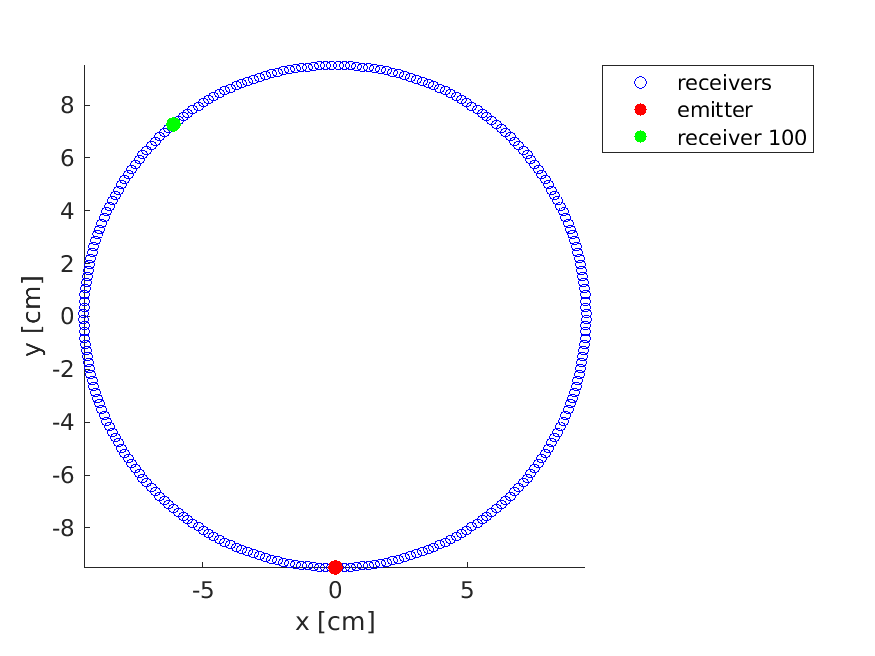
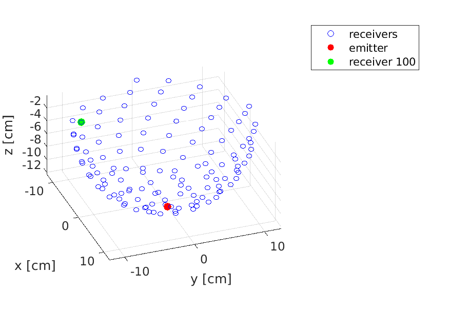
Figure 1. Transducers: (a) 2D medium, (b) 3D medium.

Three different source pulses $q_{\{s,p\}}^{\text{point}}$ were used, and the simulations were performed within a time $\big{[}0,T]$ with $T=163.26\ \mu s$. $q_{\{s,p\}}^{\text{point}}$ means a nonphysical source, which can be either $s$ or $(\partial/\partial\bm{n})p$, and is defined on a single point. Figures 2, 2 and 2 show the source pulses 1, 2 and 3, respectively. A low-pass filter was applied on each source using the filterTimeSeries.m function in the k-Wave to ensure that the frequency spectrum of the pulse be smaller than the maximum frequency supported by the computational grid. The maximum absolute amplitudes of the pulses were then normalised. The source pulses are shown after low-pass filtering and normalisation in amplitude. The maximum frequency supported by the grid for the wave simulation can be determined by the Shannon-Nyquist limit [2]. For a homogeneous medium with sound speed $c$, the maximum supported frequency is determined by [5]

$$f_{\text{max}}=\frac{c}{2\Delta x}.$$ (60)

Here, considering that $\Delta x=0.4$ mm and $c=1500\text{m}{s}^{-1}$ and homogeneous, the computed $f_{\text{max}}$ was $1.875$ MHz. The simulations were done using different Courant–Friedrichs–Lewy (CFL) numbers. The simulation for source pulse 1 was performed using a CFL number 0.1, which gives a time spacing $\Delta t=25.25$ $ns$, equivalent to a sampling rate of $39.6$ MHz. The simulation for source pulse 2 was performed using a CFL number 0.2, which gives a time spacing $50.51$ ns, equivalent to a sampling rate of 19.80 MHz. The simulation 3 was performed using a CFL number 0.3, which is equivalent to a time spacing $75.76$ ns and a sampling rate of 13.20 MHz. Figures 2, 2 and 2 show the amplitude and phase of the source pulses in the frequency domain for the simulations 1, 2 and 3, respectively. For each simulation, the simulated field was recorded at the sampled times and on the receivers, and the recorded signals in time on the receivers were then decomposed into the frequency components (phase and amplitude) using a Fourier Transform operator. As a benchmark, this nonphysical solution field was also analytically calculated using the frequency-domain formula (56), in which the Green’s function was calculated using Eq. (24).

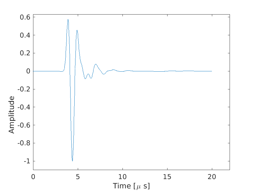
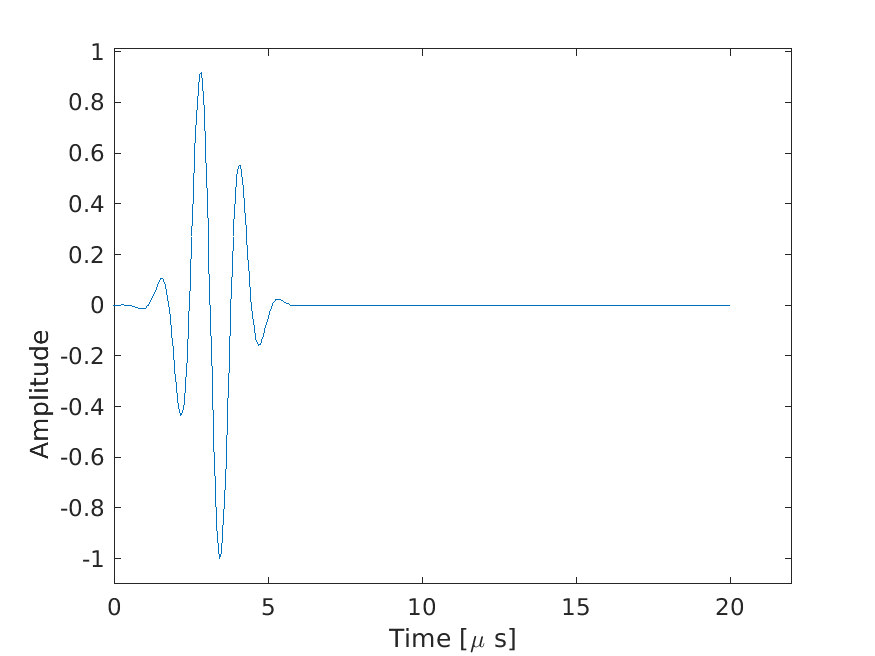
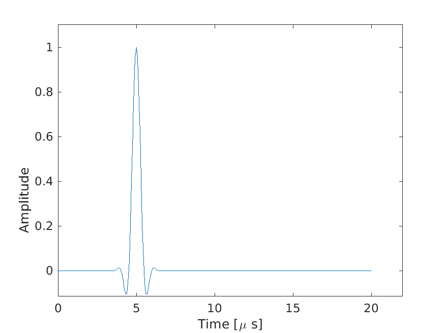
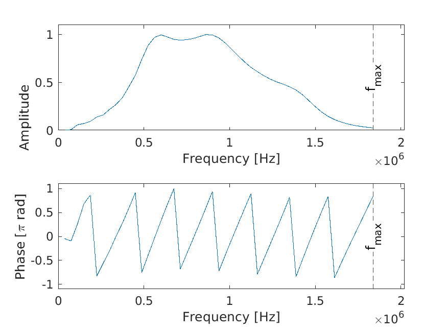
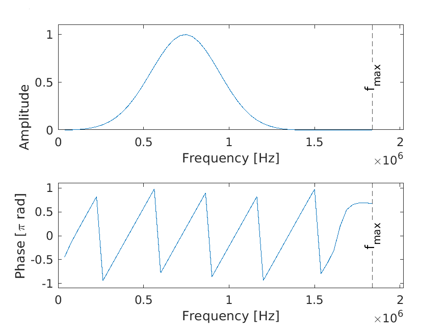
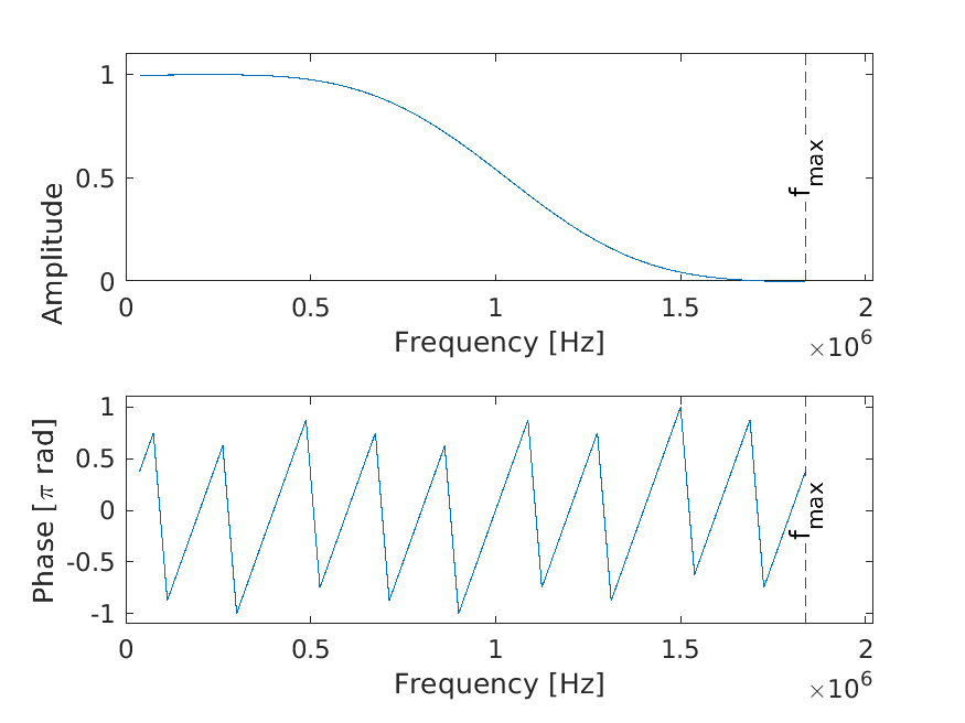
Figure 2. 2D medium. The time-domain source pulses on a single point ($q_{\{s,p\}}^{\text{point}}$): a) 1, b) 2 and c) 3. The frequency-domain amplitude and phase of the point sources: d) 1, e) 2 and f) 3.

Figures 3, 3 and 3 show the amplitude of the solution field induced by a radiation of the emitter (the red circle in figure 1) and recorded on the receiver 100 (the green circle in figure 1) as a function of temporal frequency, when the source pulses 1, 2 and 3 were used, respectively. As shown in these figures, the amplitudes of the solution field approximated using algorithm 1 and a mass source computed using Eq. (59) (the modified k-Wave) match the amplitudes analytically calculated using the Green’s formula (56) for all frequencies, but the amplitudes approximated using the original k-Wave are different from the analytically calculated amplitudes. It must be reminded that the details about the full-discretisation of the wave equation in the original k-Wave is given in the k-Wave manual [5], section 2.4, or [45], Algorithm 1. Specifically, the step taken for including the mass source has been described in the k-Wave manual [5], section 2.4, equations (2.18) and (2.19), or [45], Algorithm 1, line 5.

In the same way, figures 3, 3 and 3 show the phases of the solution field recorded on the receiver 100, when the source pulses 1, 2 and 3 were used, respectively. The phases were wrapped to $\big{[}-\pi,\pi\big{]}$ rad. As shown in the these figures, the phases approximated by the modified k-Wave and phases analytically calculated using the frequency-domain Green’s formula (56) match for all frequencies, but the phases approximated using the original k-Wave are different from the analytically calculated phases.

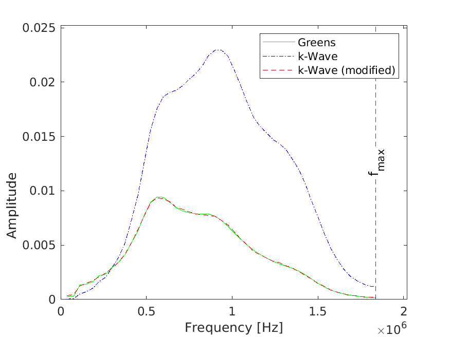
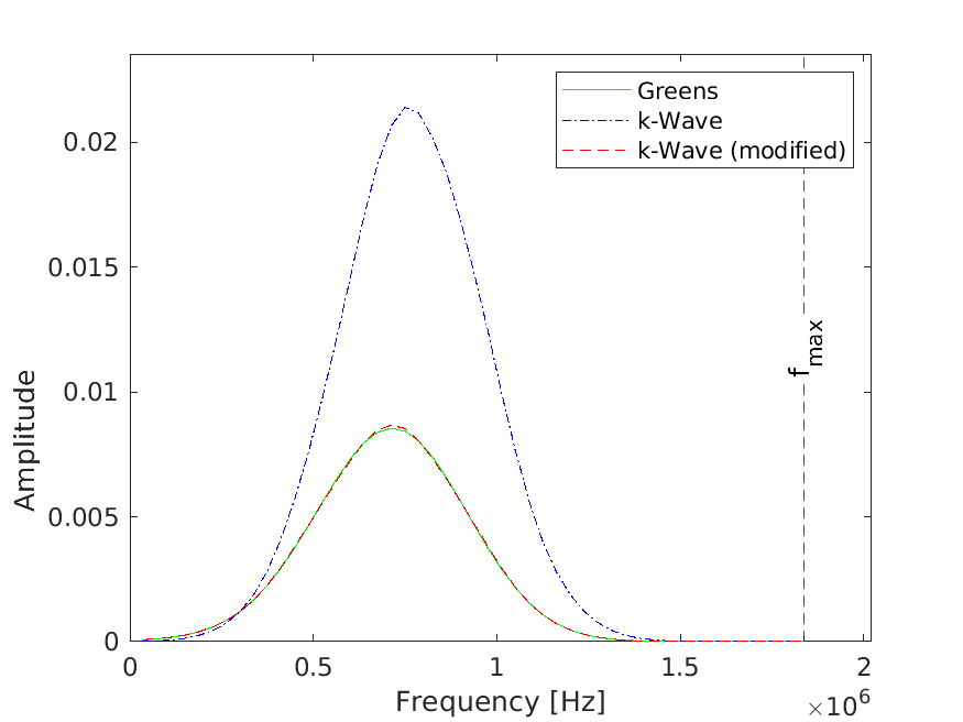
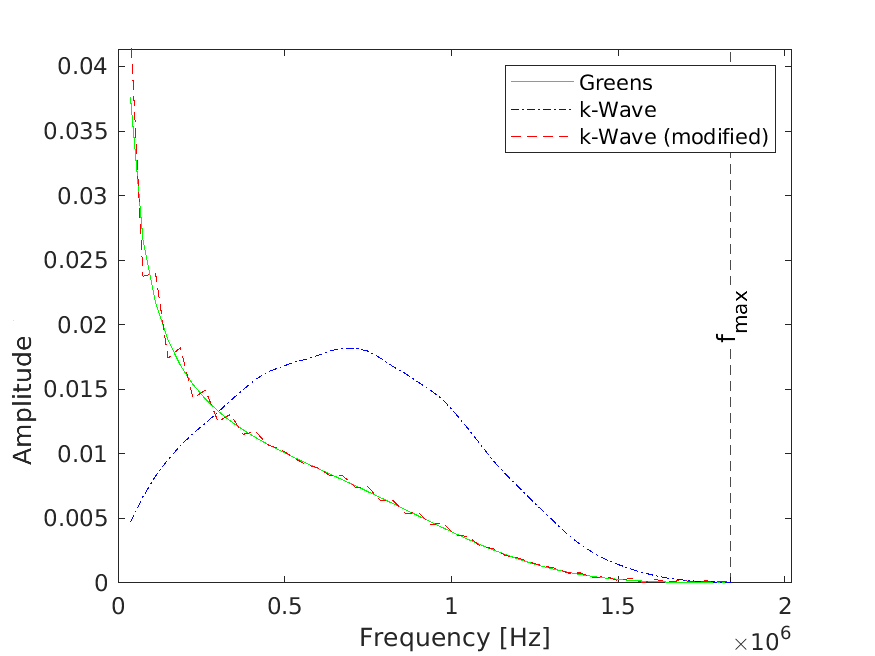
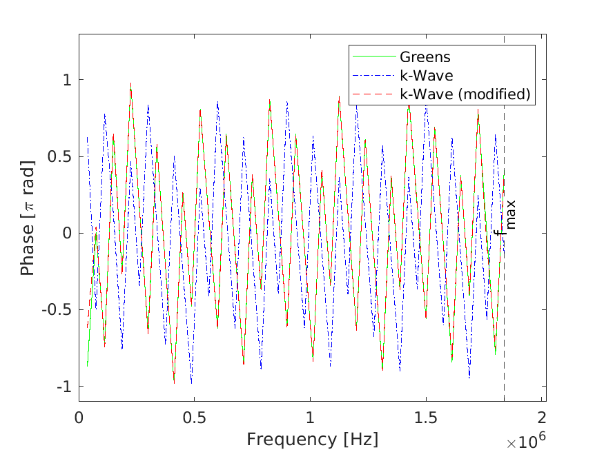
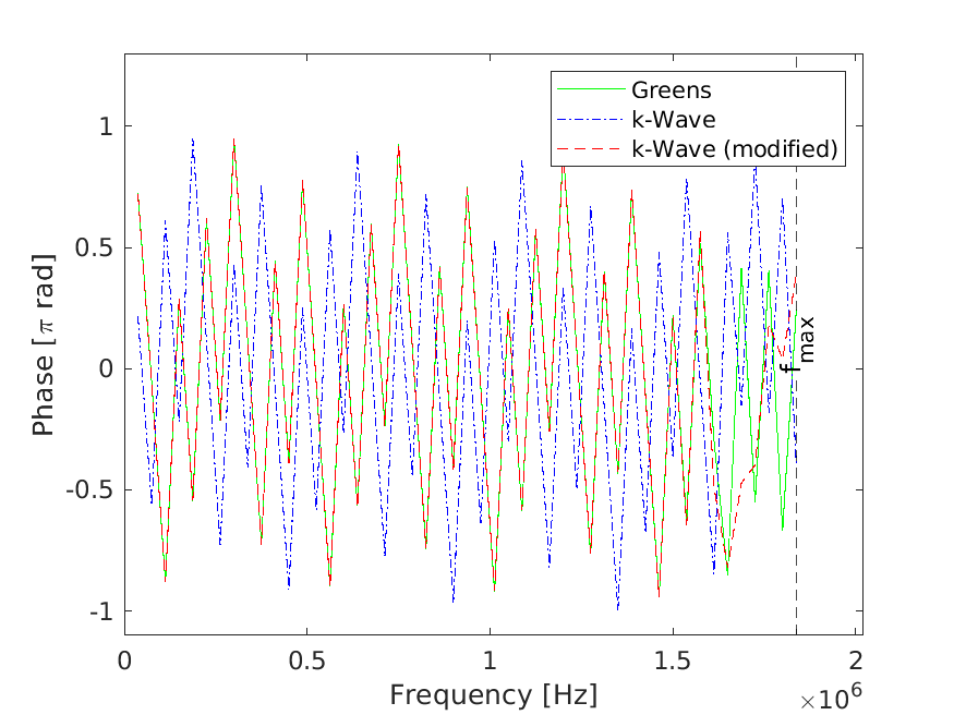
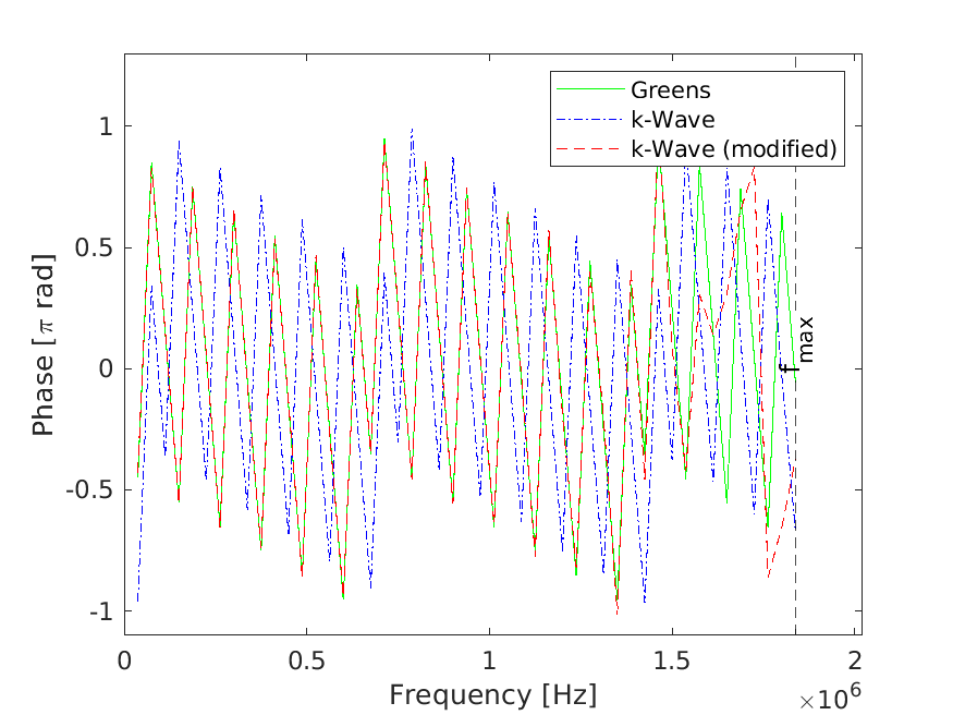
Figure 3. 2D medium. The solution field recorded on the point receiver 100 after radiation of the point source (emitter). The solution field was decomposed into amplitude and phase in the frequency domain. Amplitudes for simulation experiments: a) 1, b) 2 and c) 3. Because the source is defined on a single point, the quantities of the wave simulation are not physical and the solution field is not pressure. But an integration over a distribution of point sources using the derived formulae in section 4.2 and their discretisation discussed in section 4.3 will provide a solution field in terms of the pressure and with the units of Pascal. Phases for simulation experiments: d) 1, e) 2 and f) 3. The phases were wrapped to $\big{[}-\pi,\pi\big{]}$ rad.

Figures 4, 4 and 4 show the amplitudes of the solution field recorded on all the receivers as a function of distance of receivers to the emitter, when the source pulses 1, 2 and 3 were used, respectively. In these figures, the amplitudes were computed at the single frequency $f_{\text{max}}/2=0.92$ MHz. As shown in these figures, for all these source pulses, the amplitudes computed using the modified k-Wave simulation (red plot) match the analytic solution to the wave equation using the Green’s function (green plot), but the amplitudes computed by the original k-Wave (blue plot) are different from the analytically calculated amplitudes. In the same way, figures 4, 4 and 4 show the phase of the solution field recorded on all the receivers, when the source pulses 1, 2 and 3 were used, respectively. The phases were wrapped to $\big{[}-\pi,\pi\big{]}$ rad. As shown in these figures, the phases approximated by the modified k-Wave match the analytically calculated phases on all the receivers, but the phases approximated using the original k-Wave are different from the analytically calculated phases .

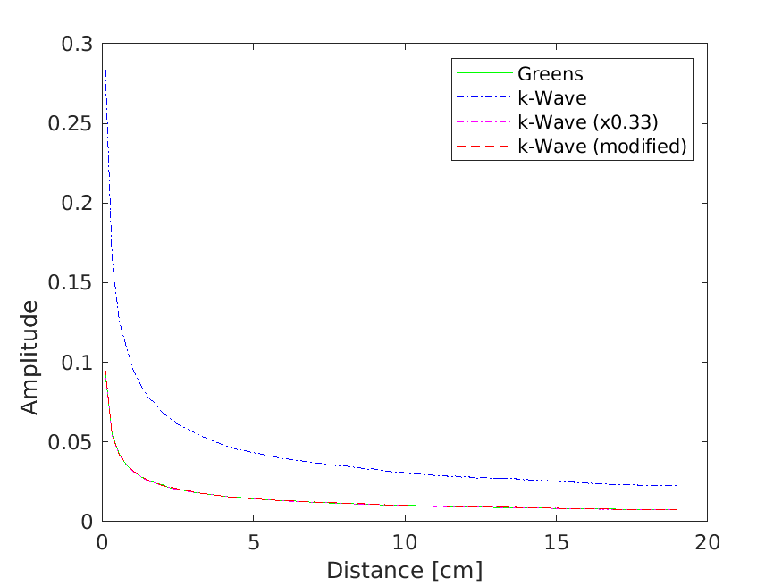
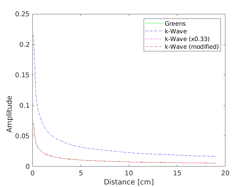
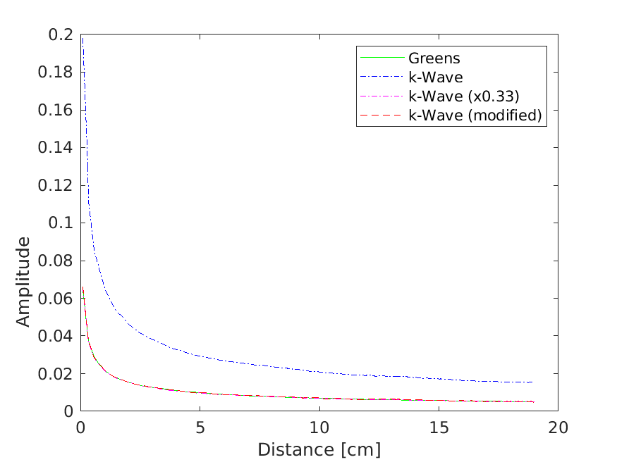
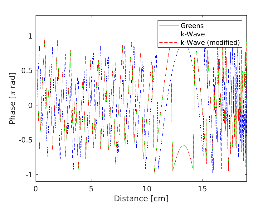
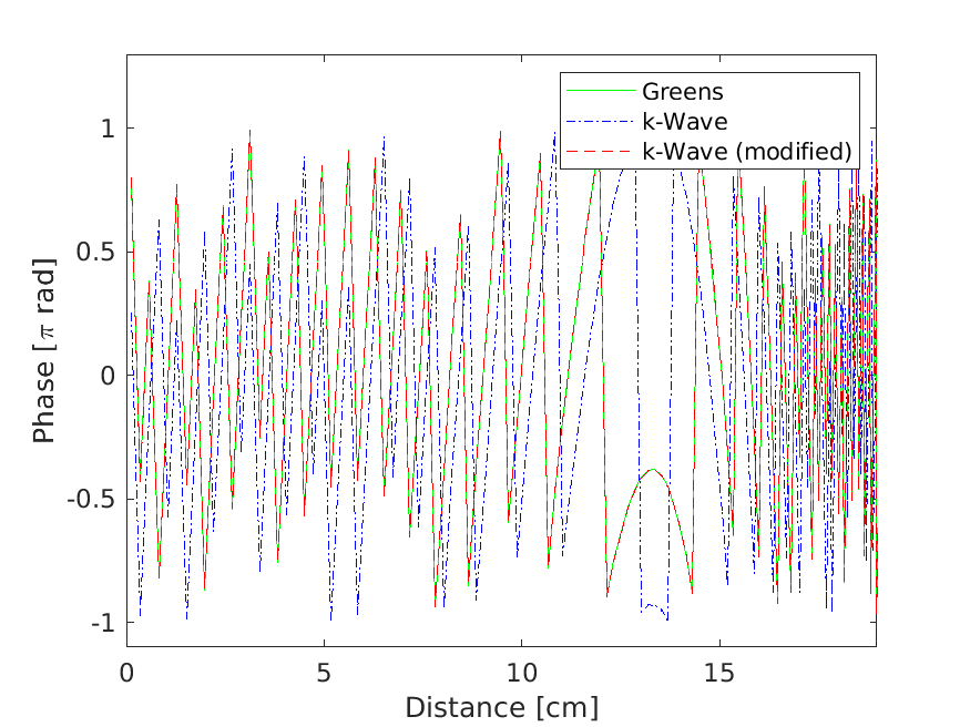
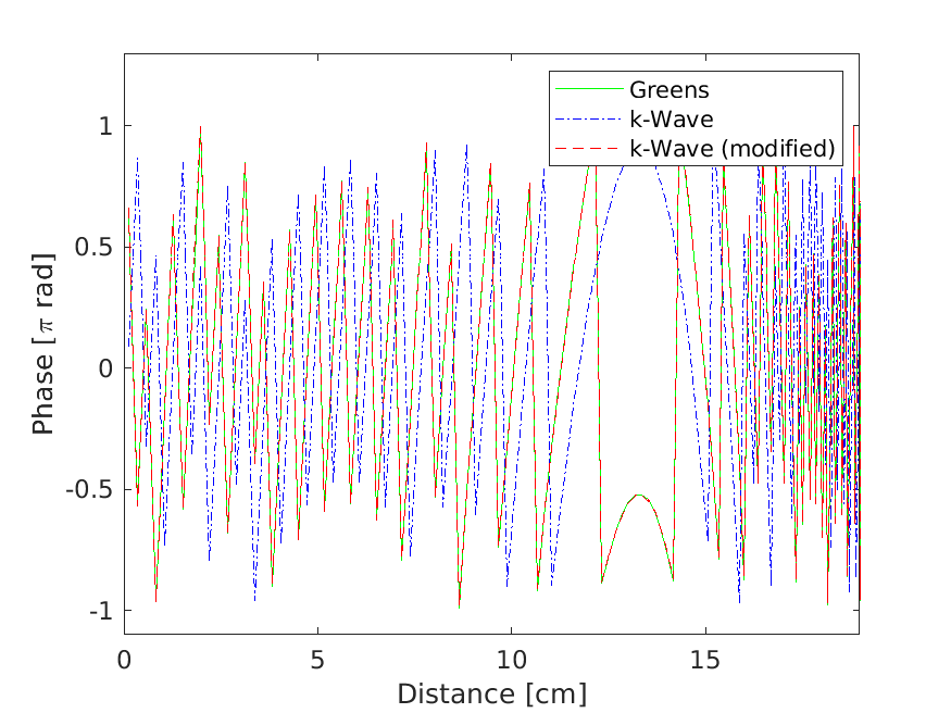
Figure 4. 2D medium. The solution field recorded on all the receivers after radiation of the point source (emitter). The solution field was decomposed into amplitude and phase in the frequency domain, and is shown at the single frequency $f_{\text{max}}/2$ as a function of distances of the receivers to the emitter. Amplitudes for simulation experiments: a) 1, b) 2 and c) 3. Phases for simulation experiments: d) 1, e) 2 and f) 3. The phases were wrapped to $\big{[}-\pi,\pi\big{]}$ rad.

5.2. Wave simulation for a 3D medium

The wave simulations were performed on a grid with the same grid spacing $0.5$ mm along all the Cartesian coordinates. The grid spacing must be small sufficiently that the frequency range of the source is supported by the grid. One emitter and 256 receivers were placed on a hemisphere with a radius of 12.35 cm, as shown in figure 1. The emitter was placed at the bottom of the hemisphere on the position $\bm{x}_{j_{0}}=\big{[}1.54,0,-12.25\big{]}\text{cm}$. Figure 1 shows the emitter by the red colour and the receivers by the blue colour. The interpolations between the position of the emitter/receivers and the grid points were performed using the formula (50) [3]. The sound speed was set 1500 $\text{ms}^{-1}$ and homogeneous. The wave simulations were performed using three different sources $q_{\{s,p\}}^{\text{point}}$ for a time duration $T=212.2\mu s$. Figures 5, 5 and 5 show the source pulses 1, 2 and 3 in time, respectively. Here, a low-pass filter was applied on each source using the filterTimeSeries.m function in the k-Wave to ensure that the frequency spectrum of the associated pulse be smaller than the maximum frequency supported by the computational grid, and then the maximum absolute amplitudes of the pulses were normalised. The maximum frequency supported by the grid was $f_{\text{max}}=1.5$ MHz.

For the simulation using the source pulse 1, the CFL number was set 0.1, which is equivalent to a time spacing $\Delta t=31.57$ ns and a sampling rate of $31.68$ MHz. The simulation 2 was performed using the CFL number 0.2, which gives a time spacing $63.13$ ns, equivalent to a sampling rate $15.84$ MHz. The simulation using the source pulse 3 was performed using the CFL number 0.3, equivalent to a time spacing $94.70$ ns and a sampling rate of $10.56$ MHz. Figures 5, 5 and 5 show the amplitudes and phases of the sources in the frequency domain for the simulations 1, 2 and 3, respectively. Note that the approach taken for including a discretised version of the mass source in the original k-Wave has been explained in [5], section 2.4., equations (2.18) and (2.19), or [45], Algorithm 1, line 5. The taken approach in the original k-Wave for including the mass source was not clear to the author, and was thus replaced by the formula (59) to represent a nonphysical mass source for a single point. An integration using the formulae (51)-(53) over a distribution of point sources will then provide the physical quantities with physical units, as explained in sections 4.2 and 4.3.

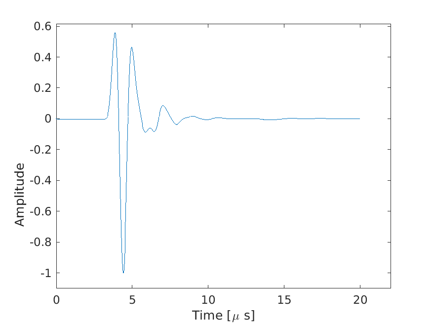
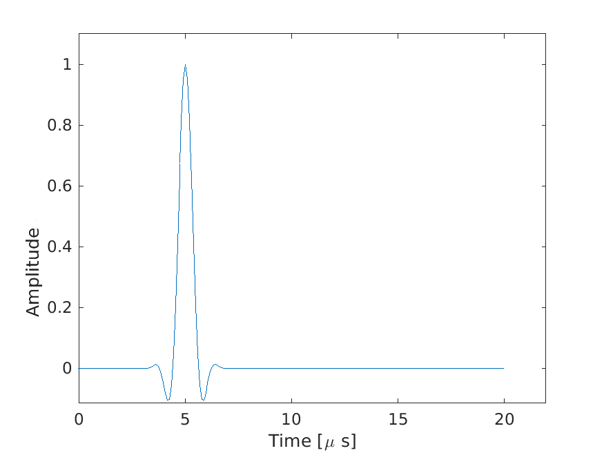
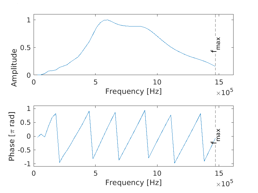
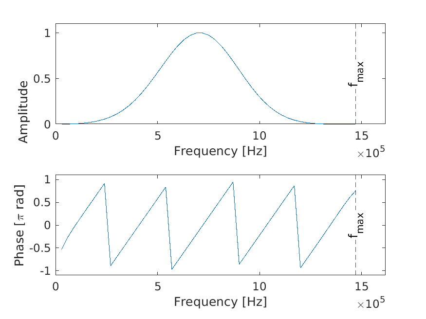
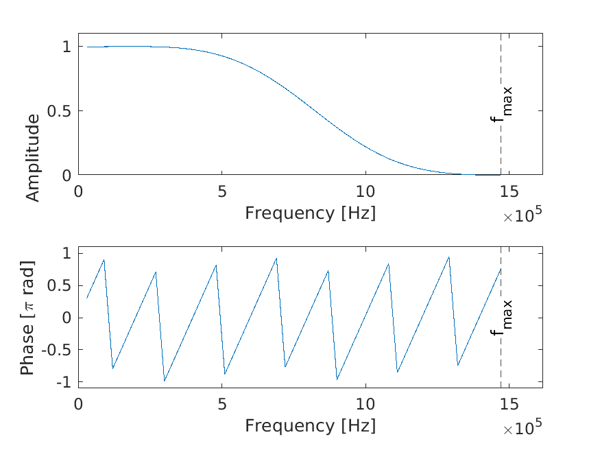
Figure 5. 3D medium. The time-domain source pulses on a single point ($q_{\{s,p\}}^{\text{point}}$): a) 1, b) 2 and c) 3. The frequency-domain amplitude and phase of the point sources: d) 1, e) 2 and f) 3.

For each simulation, the solution field was recorded on the receivers in time. The recorded time-domain signal on each receiver was then decomposed into the frequency components (phase and amplitude) using a Fourier Transform operator. The solution field was also calculated analytically in the frequency domain using the formula (56), in which the source is transferred to the frequency domain using the same Fourier operator, and the causal (or outgoing) Green’s function is calculated using (22). Figures 6, 6 and 6 show the frequency-domain amplitudes of the solution field recorded on receiver 100 (the green circle in figure 1) after excitation of emitter (the red circle in figure 1) using the source pulses 1, 2 and 3, respectively. Because the amplitudes computed by the original k-Wave (the blue plot) are much smaller than the amplitudes calculated using Eq. (56) (green plot), a variant of the original k-Wave amplitudes enlarged by a factor 666.7 was also shown by the magenta colour for a better visualisation.

As shown in these figures, the amplitudes approximated using the modified k-Wave match the amplitudes calculated analytically using the Green’s formula (56) for all frequencies. In addition, considering Eq. (22), the amplitude of the Green’s function in a 3D medium depends only on the distances, and is not changed with frequency. Note that for a nonabsorbing medium, the amplitude of the Green’s function represents only geometrical attenuation. (cf. [64] and [65].) Therefore, the fact that the amplitude of the Green’s function in (22) is independent of frequency implies that the shape of the ultrasonic pulse should remain unchanged after propagation in the medium. A comparison between the amplitudes of the source pulses in figures 5, 5 and 5 and the approximated amplitudes of the solution field on the receiver 100 in the respective figures 6, 6 and 6 shows that the geometrical attenuation approximated by the k-Wave has changed with frequency, but the attenuation approximated using the modified k-Wave has remained unchanged with frequency. For example, for simulation 1, the maximum amplitude of the source in the frequency domain, the amplitude analytically calculated using the Green’s formula, and the amplitude approximated using the modified k-Wave in the frequency domain are all close to 0.6 MHz, but the maximum amplitude approximated using the original k-Wave has been shifted to about 0.9 MHz, as shown in figure 6 by the magenta plot. Figures 6, 6 and 6 show the phases of the solution field recorded on the receiver 100, when the source pulses 1, 2 and 3 were used, respectively. The phases were wrapped to $\big{[}-\pi,\pi\big{]}$ rad. As shown in these figures, the phases approximated using the modified k-Wave and the phases calculated using the Green’s formula match for all frequencies, but the phases approximated using the original k-Wave are different.

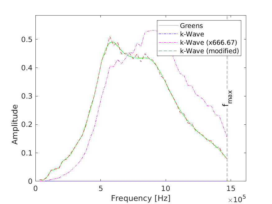
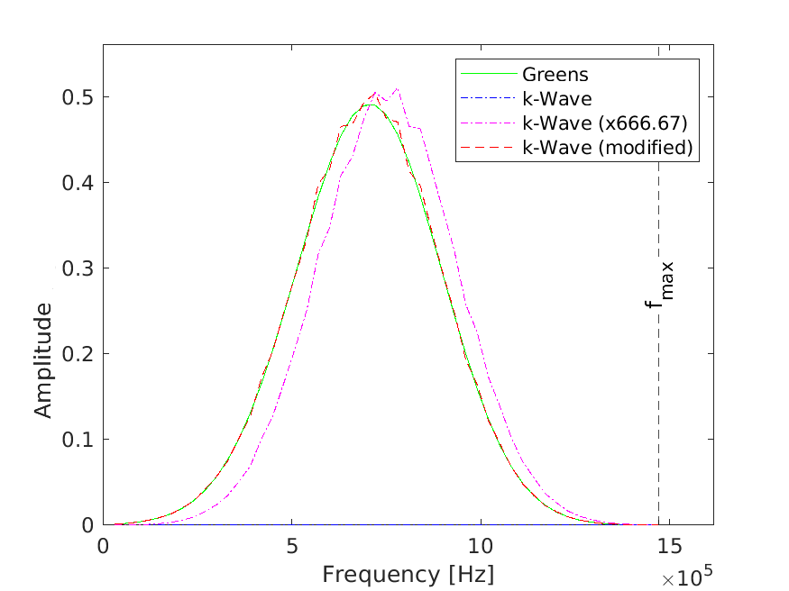
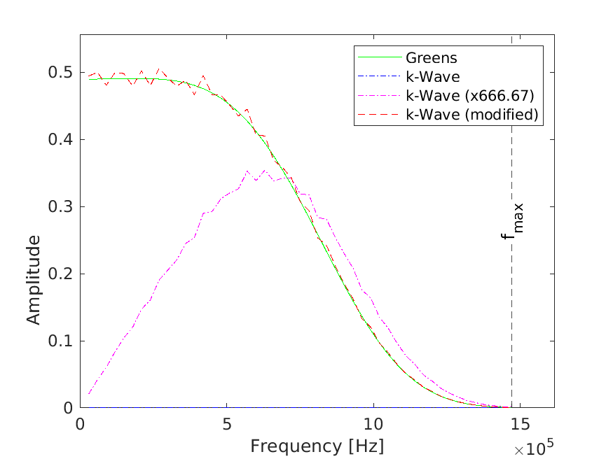
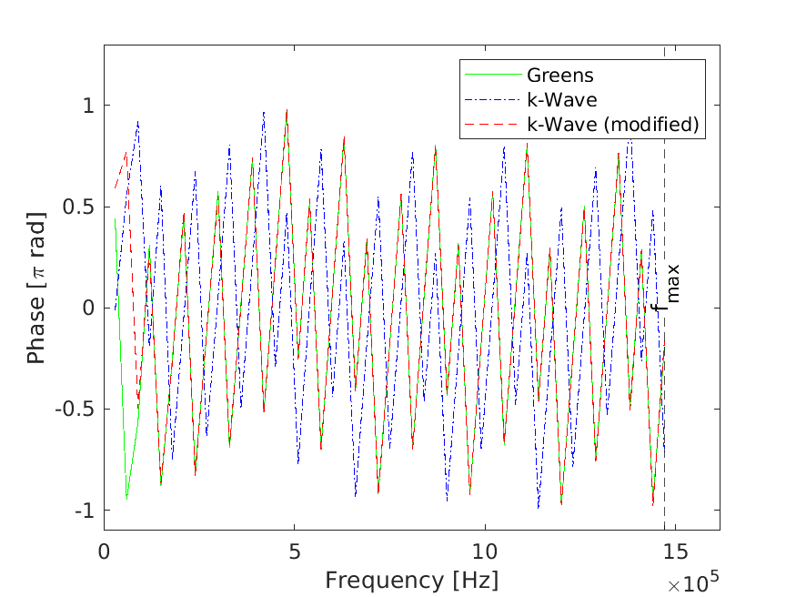
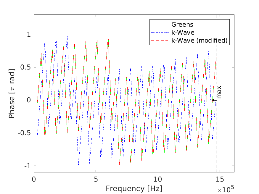
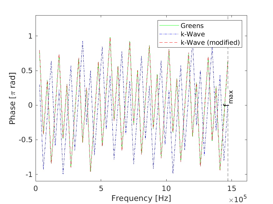
Figure 6. 3D medium. The solution field recorded on the point receiver 100 after radiation of the point source (emitter). The solution field was decomposed into amplitude and phase in the frequency domain. Amplitudes for simulation experiments: a) 1, b) 2 and c) 3. Because the source is defined on a single point, the quantities of the wave simulation are not physical and the solution field is not pressure. But an integration over a distribution of point sources using the derived formulae in section 4.2 will provide a solution field in terms of pressure and with the units of Pascal. Phases for simulation experiments: d) 1, e) 2 and f) 3. The phases were wrapped to $\big{[}-\pi,\pi\big{]}$ rad.

Figures 7, 7 and 7 show the amplitudes of the solution field recorded on all the receivers as a function of distances of receivers to the emitter, when the source pulses 1, 2 and 3 were used, respectively. In these figures, the amplitudes were computed at the single frequency $f_{\text{max}}/2$ MHz. Because the amplitudes computed by the original k-Wave (blue plot) are much smaller than the Green’s function (green plot), they are enlarged by a factor 666.7 for a better visualisation (magenta plot). As shown in these figures, using all the chosen pluses, the amplitudes computed using the modified k-Wave (red plot) match the analytically calculated amplitudes (green plot), but the amplitudes computed by the original k-Wave are different from the analytic solution. In the same way, figures 7, 7 and 7 show the phases, which have been wrapped to $\big{[}-\pi,\pi\big{]}$ rad. As shown in these figures, the phases approximated by the modified k-Wave match the analytically calculated phases for all the receivers, but the phases approximated using the original k-Wave are different.

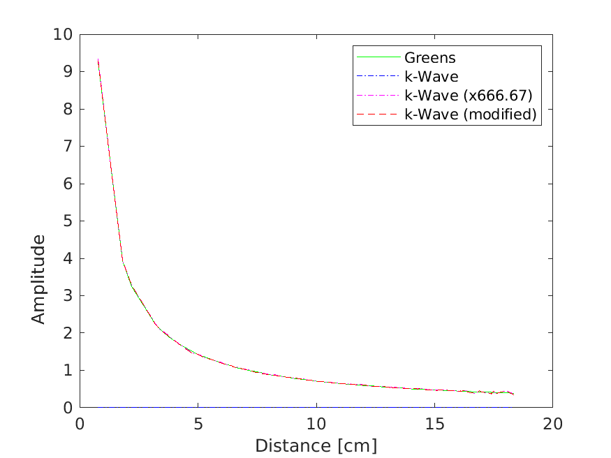
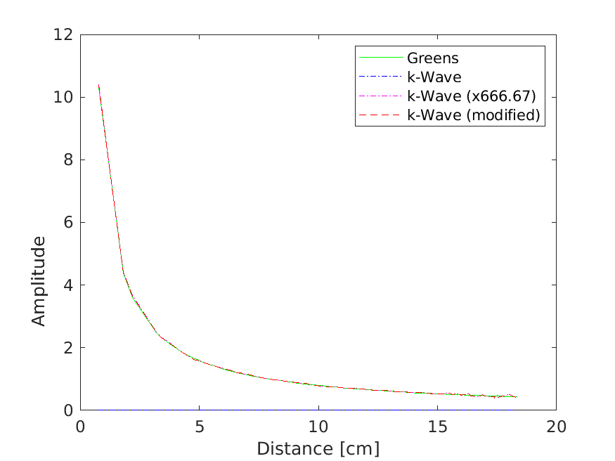
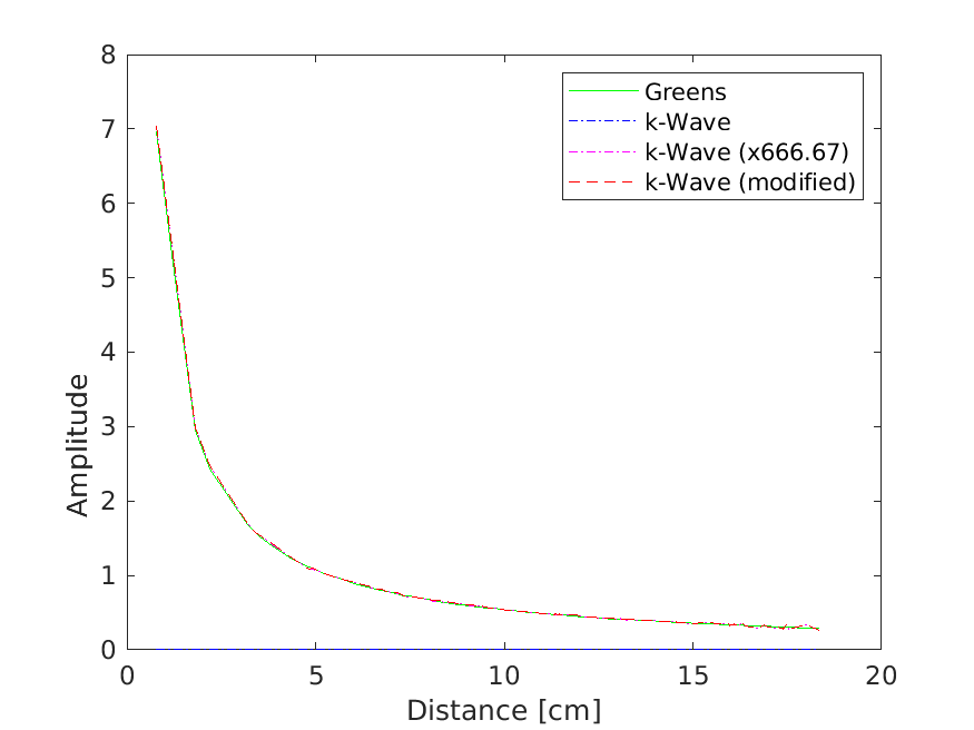
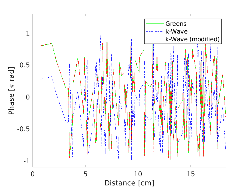
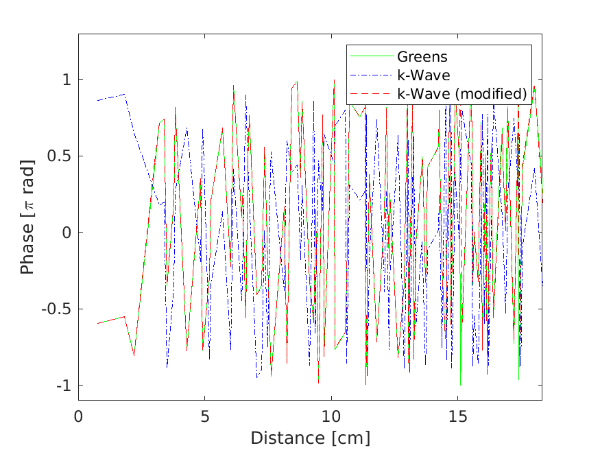
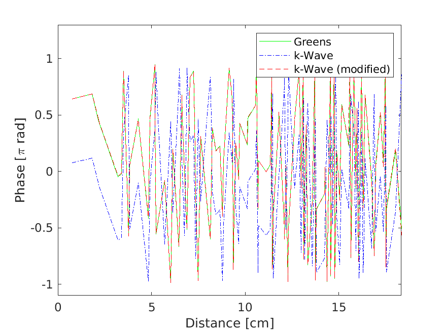
Figure 7. 3D medium. The solution field recorded on all the receivers after radiation of the point source (emitter). The solution field was decomposed into amplitude and phase in the frequency domain, and is shown at the single frequency $f_{\text{max}}/2$ as a function of distances of the receivers to the emitter. Amplitudes for simulation experiments: a) 1, b) 2 and c) 3. Phases for simulation experiments: d) 1, e) 2 and f) 3. The phases were wrapped to $\big{[}-\pi,\pi\big{]}$ rad.

6. Discussion

This manuscript explained step by step approaches for numerical approximations to analytic solutions to the wave equation. It was shown theoretically and numerically that the numerical approximations to the wave equation is equivalent to representing the wavefield solution as superposition of actions of Green’s function on a volumetric or surface source over the space and time of support of the source. The author felt that this very important equivalence may have not been paid due attention.

The primary formula (11) solves a causal variant of the wave equation (1) or its canonical form (2), and represents the propagated pressure wavefield $p$ directly in terms of the radiation source $s$. This solution of the wave equation is the most common solution used in Geophysics and Biomedical studies, for example this solution was used in the developed ray-born inversion approaches for quantitative ultrasound tomography [64, 65]. For practical studies, it may be more convenient to represent the wavefield in terms of a surface source. Correspondingly, the Kirchhoff-Helmholtz formula is used to represent the wavefield in terms of a source defined over a finite closed surface, and the Rayleigh-Sommerfeld formula was derived for planar sources.

It was shown that modelling the mass source is the key step for accurate numerical approximations matching the derived analytic solutions to the wave equation. Failure to understand the equivalence between the analytic and numerical solutions to the wave equation may lead to taking confusing approaches for defining the mass source or integration of the mass source over a surface. For example, in [5], section 2.4, equations (2.18) and (2.19) and the paragraph above, the approach taken for including the mass source in the discretised formulae for solving the wave equation has led to inconsistencies in the units of the derived equations. In the k-Wave manual [5], equations (2.18) and (2.19), the mass source is claimed to be defined in terms of surface sources of types velocity and pressure, respectively. However, the analytic approaches taken for deriving these discretised formulae are unknown to the author. In [45], Algorithm 1, line 5, the same equation as Eq. (2.19) in the k-Wave manual [5] was used for defining the mass source, but the source was defined in terms of $s$, instead of the pressure in Pascal, so it is not clear to the author if Eq. (2.19) in the k-Wave manual [5] is in terms of $s$ or $p$ in Pascal, although both assumptions do not make sense to the author. Another step which was not understood by the author is the approach taken in [66], section II. C, for numerically integrating a distribution of source over a surface defined on a three-dimensional computational grid. The author felt that more rigorous approach may be required for accurately modelling and including time-varying source in the wave equation. Nevertheless, the k-Wave Version 1.3, was still used, and the step for discretising the gradient of fields was kept unchanged, but the steps for including the mass source were changed based on the procedure explained in section 4. The proposed approach is based on applying triangulation on the space of the volumetric or surface source, and then mapping the space of the source onto the regular computational grid via a change of variable of integral in space. Note that compared to the numerical integration approach in [66], section II, C, the triangulation step included in our proposed approach for modelling the mass source is more accurate, because it is not limited to a mesh with equidistant nodes. Therefore, the triangulation will provide more degrees of freedom for modelling the source and can improve spatial resolution near sharp boundaries.

The numerical approach proposed for including the time-varying source in the wave equation was validated via a comparison with the associated analytic solutions. For the sake of simplicity and generality, the comparison was done for a source defined on a single point. The match obtained between the analytical and numerical solutions to the wave equation is very important for future studies in the field of biomedical acoustics.

7. Conclusion

This manuscript simply shared the scientific experience of the author about how the step for inclusion of time-varying source in the wave equation should be treated for obtaining numerical solutions matching the common analytic solutions to the acoustic wave equation.

References

- [1] T. D. Mast, L. P. Souriau, D. -L. D. Liu, M. Tabei, A. I. Nachman and R. C. Waag, “A k-space method for large-scale models of wave propagation in tissue”, IEEE Trans. Ultrason. Ferroelectr. Freq., vol. 48, no. 2, pp. 341-354, March 2001, doi: 10.1109/58.911717.
- [2] M. Tabei, T. D. Mast, and R. C. Waag, “A k-space method for coupled first-order acoustic propagation equations”, J. Acoust. Soc. Am. vol. 111, pp. 53–63, 2002.
- [3] B. E. Treeby and B. T. Cox, “k-Wave: MATLAB toolbox for the simulation and reconstruction of photoacoustic wave fields”, J. Biomed. Opt. vol. 15, no. 2, 021314, 2010.
- [4] S. Holm ans S.P. Näsholm, “A causal and fractional all-frequency wave equation for lossy media”, The Journal of the Acoustical Society of America, Vol. 130, no. 4, pp. 2195-2202, 2011.
- [5] B. Treeby and B. Cox, k-Wave user manual, “A Matlab toolbox for the time domain simulation of acoustic wave fields”, Version 1.1, 27th August 2016 (the last version).
- [6] M. J. Bencomo and W. W. Symes, “Discretization of multipole sources in a finite difference setting for wave propagation problems”, Journal of Computational Physics, vol. 386, pp. 296-322, 2019.
- [7] A. Siahkoohi, M. Louboutin and F. J. Herrmann, “The importance of transfer learning in seismic modeling and imaging”, Geophysics, Vol. 84, no. 6, pp. A47-A52, 2019, https://doi.org/10.1190/geo2019-0056.1.
- [8] A. Javaherian, F. Lucka and B. Cox, “Refraction-corrected ray-based inversion for three-dimensional ultrasound tomography of the breast”, Inverse Problems, vol. 36, no. 12, 125010, 2020.
- [9] T. Furuya and R. Potthast, “Inverse medium scattering problems with Kalman filter techniques”, Inverse Problems, Vol. 38, no. 9, 095003, 2022.
- [10] S. Bhattacharyya, M. V. de Hoop, V. Katsnelson and G. Uhlmann, “Recovery of wave speeds and density of mass across a heterogeneous smooth interface from acoustic and elastic wave reflection operators”, GEM-International Journal on Geomathematics, Vol. 13, no. 1, 2022.
- [11] S. Holm, S. N. Chandrasekaran and S. P. Näsholm, “Adding a low frequency limit to fractional wave propagation models”, Front.Phys., 11:1250742.2023.https://doi.org/10.3389/fphy.2023.1250742.
- [12] H. Chauris and M. Farshad, “Seismic differential semblance-oriented migration velocity analysis — Status and the way forward”, Geophysics, Vol. 88, no. 6, pp. U81-U100, 2023.
- [13] M. Bader, R. G. Clapp, K. T. Nihei, and B. Biondi, “Moment tensor inversion of perforation shots using distributed-acoustic sensing”, Geophysics,Vol. 88, no. 6, pp. 1-36, 2023. https://doi.org/10.1190/geo2021-0661.1.
- [14] M. Papadopoulou, B. Brodic, E. Koivisto and A. Kaleshova, M. Savolainen, P. Marsden, and L. V. Socco, “High-resolution static corrections derived from surface-wave tomography: Application to mineral exploration”, Geophysics, Vol. 88, no. 6, B317-B328, 2023.
- [15] M. V. Eaid, S. D. Keating, K. A. Innanen, M. Macquet and D. Lawton, “Field assessment of elastic full-waveform inversion of combined accelerometer and distributed acoustic sensing data in a vertical seismic profile configuration”, Geophysics, vol. 88, no. 6, pp. WC163-WC180, 2023.
- [16] B. Kaltenbacher and W. Rundell, “On the simultaneous reconstruction of the nonlinearity coefficient and the sound speed in the Westervelt equation”, Inverse Problems, Vol. 39, no. 10, p. 105001, 2023, DOI 10.1088/1361-6420/aceef2.
- [17] G. Uhlmann and Y. Zhang, “An inverse boundary value problem arising in nonlinear acoustics”, SIAM Journal on Mathematical Analysis, Vol. 55, no. 2, pp. 1364-1404, 2023.
- [18] B. Kaltenbacher and V. Nikolić, The vanishing relaxation time behavior of multi-term nonlocal Jordan–Moore–Gibson–Thompson equations, Nonlinear Analysis: Real World Applications, Vol. 76, pp. 103991, 2024, https://doi.org/10.1016/j.nonrwa.2023.103991.
- [19] J.Qian, P.Stefanov, G.Uhlmann and H.Zhao, “An Efficient Neumann series–based algorithm for thermoacoustic and photoacoustic tomography with variable sound speed”, SIAM Journal on Imaging Sciences, Vol.4, no.3, 2011. doi: 10.1137/100817280.
- [20] T.Tarvainen, B.T.Cox, J.Kaipio, and S.R. Arridge, “Reconstructing absorption and scattering distributions in quantitative photoacoustic tomography”, Inverse Problems, Vol. 28, 2012 ,p.084009.
- [21] R.Kowar and O.Scherzer, “Attenuation Models in Photoacoustics”. In: H. Ammari (eds) Mathematical Modeling in Biomedical Imaging II. Lecture Notes in Mathematics, Vol. 2035, 2012. Springer, Berlin, Heidelberg. https://doi.org/10.1007/978-3-642-22990-94.
- [22] X.L.Dean-Ben, A.Buehler, V.Ntziachristos and D.Razansky, “Accurate model-based reconstruction algorithm for three-dimensional optoacoustic tomography”, IEEE Transactions on Medical Imaging, Vol.31, no.10, pp.19221928, 2012.
- [23] S.Arridge, M.Betcke, B.Cox, F.Lucka and BE Treeby, “On the adjoint operator in photoacoustic tomography”, Inverse Problems, vol.32, 115012, 2016.
- [24] M.Haltmeier and L.V.Nguyen, “Analysis of iterative methods in photoacoustic tomography with variable sound speed”, SIAM Journal on Imaging Sciences, Vol.10,no.2,2017, doi: 10.1137/16M1104822.
- [25] J. A. Guggenheim, J. Li, T. J. Allen, R. J. Colchester, S. Noimark, O. Ogunlade, I. P. Parkin, I. Papakonstantinou, A. E. Desjardins, E. Z. Zhang and P. C. Beard, “Ultrasensitive plano-concave optical microresonators for ultrasound sensing”. Nature Photon, Vol. 11, pp. 714-719, 2017. https://doi.org/10.1038/s41566-017-0027-x.
- [26] A. Javaherian and S. Holman, “A continuous adjoint for photo-acoustic tomography of the brain”, Inverse Problems, vol. 34, no. 8, p. 085003, 2018.
- [27] A.Javaherian and S.Holman, “Direct quantitative photoacoustic tomography for realistic acoustic media”, Inverse Problems,vol.35,no.8,084004,2019.
- [28] S.Antholzer, M.Haltmeier and J.Schwab, “Deep-learning for photoacoustic tomography from sparse data”, Inverse Problems in Science and Engineering, Vol.27, no.7,pp.987-1005, 2019. doi: 10.1080/17415977.2018.1518444.
- [29] S. Guan, A. A. Khan, S. Sikdar and P. V. Chitnis, “Fully dense UNet for 2-D sparse photoacoustic tomography artifact removal”, IEEE Journal of Biomedical and Health Informatics, vol. 24, no. 2, pp. 568-576, Feb. 2020, doi: 10.1109/JBHI.2019.2912935.
- [30] S. Na and L. V. Wang, “Photoacoustic computed tomography for functional human brain imaging”, Biomed. Opt. Express, Vol. 12, pp. 4056-4083, 2021.
- [31] J. Grohl, M. Schellenberg, K. Dreher and L. Maier-Hein, “Deep learning for biomedical photoacoustic imaging: A review”, Photoacoustics, Vol. 22, 100241, 2021.
- [32] E. Park, S. Park, H. Lee, M. Kang, C. Kim and J. Kim, “Simultaneous dual-modal multispectral photoacoustic and ultrasound macroscopy for three-dimensional whole-body imaging of small animals”, Photonics, Vol. 8, pp. 13, 2021.
- [33] L. Nguyen, M. Haltmeier, R Kowar, and N. Do, “Analysis for full-field photoacoustic tomography with variable sound speed”, SIAM Journal on Imaging Sciences, Vol. 15, no. 3, 2022, 10.1137/21M1463409.
- [34] S. M. Ranjbaran, H. S. Aghamiry, A. Gholami, S. Operto and K. Avanaki, “Quantitative photoacoustic tomography using Iiteratively refined wavefield reconstruction inversion: a simulation study”, in IEEE Transactions on Medical Imaging, doi: 10.1109/TMI.2023.3324922.
- [35] B. M. Afkham, K. Knudsen, A. K. Rasmussen and T. Tarvainen, “A Bayesian approach for consistent reconstruction of inclusions”, https://arxiv.org/abs/2308.13673.
- [36] M. Suhonen, A. Pulkkinen and T. Tarvainen, “One-step estimation of spectral optical parameters in quantitative photoacoustic tomography”, Proc. SPIE 12631, Opto-Acoustic Methods and Applications in Biophotonics VI, 126310D (11 August 2023); https://doi.org/10.1117/12.2675588.
- [37] H. Park, J. Yao and Y. Jing, “A frequency-domain model-based reconstruction method for transcranial photoacoustic imaging: A 2D numerical investigation”, Photoacoustics, Vol. 33, 2023, p. 100561.
- [38] F. Li, U. Villa, N. Duric and M. A. Anastasio, “A Forward Model Incorporating Elevation-Focused Transducer Properties for 3-D Full-Waveform Inversion in Ultrasound Computed Tomography”,in IEEE Transactions on Ultrasonics, Ferroelectrics, and Frequency Control, vol. 70, no. 10, pp. 1339-1354, Oct. 2023, doi: 10.1109/TUFFC.2023.3313549.
- [39] G. Y. Sandhu, C. Li, O. Roy, S. Schmidt and N. Duric, Frequency domain ultrasound waveform tomography: breast imaging using a ring transducer, Phys. Med. Biol., Vol. 60, 5381–5398, 2015.
- [40] A. V. Goncharsky and S. Y. Romanov, “Iterative methods for solving coefficient inverse problems of wave tomography in models with attenuation”, Inverse Problems, vol. 33, pp. 025003, 2017.
- [41] J. W. Wiskin, D. T. Borup, E. Iuanow, J. Klock and M. W. Lenox, “3-D Nonlinear Acoustic Inverse Scattering: Algorithm and Quantitative Results”, IEEE T ULTRASON FERR, vol. 64, no. 3, 2017.
- [42] H. S. Aghamiry, A. Gholami and Stéphane Operto, “Improving full-waveform inversion by wavefield reconstruction with the alternating direction method of multipliers”, Geophysics, Vol.84, no. 1, pp. R139–R162, 2019. doi: https://doi.org/10.1190/geo2018-0093.1.
- [43] L. Guasch, O. Calderón Agudo, M. Tang, P. Nachev, and M. Warner, “Full-waveform inversion imaging of the human brain”. Nature Digital Medicine, vol. 3, 28, 2020.
- [44] F. Faucher and O. Scherzer, Adjoint-state method for Hybridizable Discontinuous Galerkin discretization, ap30 plication to the inverse acoustic wave problem, Computer Methods in Applied Mechanics and Engineering, Vol. 31 372, 2020.
- [45] F. Lucka, M. Perez-Liva, B. E. Treeby and B. T. Cox, “High resolution 3D ultrasonic breast imaging by time-domain full waveform inversion”, Inverse Problems, Vol. 38, 025008, 2022.
- [46] F. Li, U. Villa, S. Park and M. A. Anastasio, “3-D Stochastic Numerical Breast Phantoms for Enabling Virtual Imaging Trials of Ultrasound Computed Tomography”, in IEEE Transactions on Ultrasonics, Ferroelectrics, and Frequency Control, vol. 69, no. 1, pp. 135-146, Jan. 2022, doi: 10.1109/TUFFC.2021.3112544.
- [47] I. E. Ulrich, S. Noe, C. Boehm, N K Martiartu, B Lafci, X. L. Dean-Ben, D. Razansky and A.Fitchner, “Full-waveform inversion with resolution proxies for in-vivo ultrasound computed tomography”, 2023 IEEE International Ultrasonics Symposium (IUS), Montreal, QC, Canada, 2023, pp. 1-4, doi: 10.1109/IUS51837.2023.10308297.
- [48] L. Lozenski, H. Wang, F. Li, M. Anastasio, B. Wohlberg, Y. Lin, and U. Villa, “Learned Full Waveform Inversion Incorporating Task Information for Ultrasound Computed Tomography”, in IEEE Transactions on Computational Imaging, doi: 10.1109/TCI.2024.3351529.
- [49] D. Schweizer, R. Rau, C. D. Bezek, R. A. Kubik-Huch and O. Goksel, “Robust Imaging of Speed of Sound Using Virtual Source Transmission”, in IEEE Transactions on Ultrasonics, Ferroelectrics, and Frequency Control, Vol. 70, no. 10, pp. 1308-1318, 2023.
- [50] Z. Zeng, Y. Zheng, Y. Zheng, Y. Li, Z. Shi Aand H. Sun, “Neural Born series operator for biomedical ultrasound computed Tomography”, 2023, https://arxiv.org/abs/2312.15575.
- [51] S. Operto, A. Gholami, H. S. Aghamiry, G. Guo, S. Beller, K. Aghazade, F. Mamfoumbi, L. Combe and A. Ribodetti, “Extending the search space of full-waveform inversion beyond the single-scattering Born approximation: A tutorial review”, Geophysics 2023;; Vol. 88, no. 6, pp. R671–R702. doi: https://doi.org/10.1190/geo2022-0758.1.
- [52] M. Soleimani, T. Rymarczyk and G. Kłosowski, “Ultrasound Brain Tomography: Comparison of Deep Learning and Deterministic Methods”, in IEEE Transactions on Instrumentation and Measurement, Vol. 73, pp. 1-12, 2024, Art no. 4500812, doi: 10.1109/TIM.2023.3330229.
- [53] L. Borcea, J. Garnier, A. V. Mamonov and J. Zimmerling, “Waveform inversion with a data driven estimate of the internal wave”, SIAM Journal on Imaging Sciences, Vol. 16, no. 1, pp. 280-312, 2023, https://doi.org/10.1137/22M1517342.
- [54] S. Ziegler, T. Santos and J. L. Mueller, “Regularized full waveform inversion for low frequency ultrasound tomography with a structural similarity EIT prior”, Inverse Problems and Imaging, vol. 18, no. 1, pp. 86-103, 2024, doi:10.3934/ipi.2023023.
- [55] A. Pulkkinen, B. Werner, E. Martin and K. Hynynen, “Numerical simulations of clinical focused ultrasound functional neurosurgery”, Physics in Medicine & Biology, vol. 59, no. 7, p. 1679, 2014.
- [56] A. Kyriakou, E. Neufeld, and B. Werner, G. Székely and N. Kuster, “Full-wave acoustic and thermal modeling of transcranial ultrasound propagation and investigation of skull-induced aberration correction techniques: a feasibility study”. J Ther Ultrasound, Vol. 3, no. 11, 2015. https://doi.org/10.1186/s40349-015-0032-9.
- [57] J. K. Mueller, L. Ai, P. Bansal and W. Legon, “Numerical evaluation of the skull for human neuromodulation with transcranial focused ultrasound”, J. Neural Eng., Vol. 14, p.066012 (19pp), 2017.
- [58] C. Pasquinelli, L.G. Hanson, H.R. Siebner, H.J. Lee and A. Thielscher, “Safety of Transcranial focused ultrasound stimulation: A systematic review of the state of knowledge from both human and animal studies”, Brain Stimul., Vol. 12, no. 6, pp. 1367-1380, 2019. doi: 10.1016/j.brs.2019.07.024. Epub 2019 Jul 31. PMID: 31401074.
- [59] P. Gaur, K.M. Casey, J. Kubanek, N. Li, M. Mohammadjavadi, Y. Saenz, G.H. Glover, D.M. Bouley and K.B. Pauly. “Histologic safety of transcranial focused ultrasound neuromodulation and magnetic resonance acoustic radiation force imaging in rhesus macaques and sheep”. Brain Stimul. 2020 May-Jun;13(3):804-814. doi: 10.1016/j.brs.2020.02.017. Epub 2020 Feb 21. PMID: 32289711; PMCID: PMC7196031.
- [60] T. Bancel et al., “Comparison Between Ray-Tracing and Full-Wave Simulation for Transcranial Ultrasound Focusing on a Clinical System Using the Transfer Matrix Formalism”, in IEEE Transactions on Ultrasonics, Ferroelectrics, and Frequency Control, vol. 68, no. 7, pp. 2554-2565, July 2021, doi: 10.1109/TUFFC.2021.3063055.
- [61] J-F Aubry, O. Bates, C. Boehm, K. B. Pauly, D. Christensen, C. Cueto, P. Gélat, L. Guasch, J. Jaros, Y. Jing, R. Jones, N. Li, P. Marty, H. Montanaro, E. Neufeld, S. Pichardo, G. Pinton, A. Pulkkinen, A. Stanziola, A. Thielscher, B Treeby and E. Van’t Wout, “Benchmark problems for transcranial ultrasound simulation: Inter-comparison of compressional wave models”, J. Acoust. Soc. Am., vol. 152, pp. 1003–1019, 2022.
- [62] J-F Aubry, D. Attali, M. Schafer, E. Fouragnan, C. Caskey, R. Chen, G. Darmani, E. J. Bubrick, J. Sallet, C. Butler, C. Stagg, M. Klein-Flugge, S-S Yoo, B. Treeby, L. Verhagen and K. B. Pauly, “ITRUSST Consensus on Biophysical Safety for Transcranial Ultrasonic Stimulation”, 2023, https://arxiv.org/abs/2311.05359.
- [63] A.J. Devaney, “Mathematical Foundations of Imaging, Tomography and Wavefield Inversion”. Cambridge University Press; 2012.
- [64] A. Javaherian and B. Cox, “Ray-based inversion accounting for scattering for biomedical ultrasound tomography”, Inverse Problems, vol. 37, no.11, 115003, 2021.
- [65] A. Javaherian, “Hessian-inversion-free ray-born inversion for high-resolution quantitative ultrasound tomography”, 2023, https://arxiv.org/abs/2211.00316.
- [66] E. S. Wise, B. T. Cox, J. Jaros and B. E. Treeby, “Representing arbitrary acoustic source and sensor distributions in Fourier collocation methods”, J. Acoust. Soc. of Am., vol. 146, no. 1, pp. 278-288, 2019.
- [67] M Dantuma et al, “Fully three-dimensional sound speed-corrected multi-wavelength photoacoustic breast tomography”, 2023, https://arxiv.org/abs/2308.06754.