Leveraging Unlabeled Data to Track Memorization

Abstract

Deep neural networks may easily memorize noisy labels present in real-world data, which degrades their ability to generalize. It is therefore important to track and evaluate the robustness of models against noisy label memorization. We propose a metric, called susceptibility, to gauge such memorization for neural networks. Susceptibility is simple and easy to compute during training. Moreover, it does not require access to ground-truth labels and it only uses unlabeled data. We empirically show the effectiveness of our metric in tracking memorization on various architectures and datasets and provide theoretical insights into the design of the susceptibility metric. Finally, we show through extensive experiments on datasets with synthetic and real-world label noise that one can utilize susceptibility and the overall training accuracy to distinguish models that maintain a low memorization on the training set and generalize well to unseen clean data.

1 Introduction

Deep neural networks are prone to memorizing noisy labels in the training set, which are inevitable in many real-world applications Frénay and Verleysen (2013); Zhang et al. (2016); Arpit et al. (2017); Song et al. (2020a); Nigam et al. (2020); Han et al. (2020); Zhang et al. (2021a); Wei et al. (2021). Given a new dataset that contains clean and noisy labels, one refers to the subset of the dataset with correct labels (respectively, with incorrect labels due to noise), as the clean (respectively, noisy) subset. When neural networks are trained on such a dataset, it is important to find the sweet spot from no fitting at all to fitting every sample. Indeed, fitting the clean subset improves the generalization performance of the model (measured by the classification accuracy on unseen clean data), but fitting the noisy subset, referred to as “memorization”, degrades its generalization performance. New methods have been introduced to address this issue (for example, robust architectures Xiao et al. (2015); Li et al. (2020), robust objective functions Li et al. (2019); Ziyin et al. (2020), regularization techniques Zhang et al. (2017); Pereyra et al. (2017); Chen et al. (2019); Harutyunyan et al. (2020), and sample selection methods Nguyen et al. (2019)), but their effectiveness cannot be assessed without oracle access to the ground-truth labels to distinguish the clean and the noisy subsets, or without a clean test set.

Our goal in this paper is to track memorization during training without any access to ground-truth labels. To do so, we sample a subset of the input data and label it uniformly at random from the set of all possible labels. The samples can be taken from unlabeled data, which is often easily accessible, or from the available training set with labels removed. This new held-out randomly-labeled set is created for evaluation purposes only, and does not affect the original training process.

First, we compare how different models fit the held-out randomly-labeled set after multiple steps of training on it. We observe empirically that models that have better accuracy on unseen clean test data show more resistance towards memorizing the randomly-labeled set. This resistance is captured by the number of steps required to fit the held-out randomly-labeled set. In addition, through our theoretical convergence analysis on this set, we show that models with high/low test accuracy are resistant/susceptible to memorization, respectively.

Building on this result, we then propose an easy-to-compute metric that we call susceptibility to noisy labels, which is the difference in the objective function of a single mini-batch from the held-out randomly-labeled set, before and after taking an optimization step on it. At each step during training, the larger this difference is, the more the model is affected by (and is therefore susceptible to) the noisy labels in the mini-batch. Figure LABEL:fig:figure1 (bottom/middle left) provides an illustration of the susceptibility metric. We observe a strong correlation between the susceptibility and the memorization within the training set, which is measured by the fit on the noisy subset. We then show how one can utilize this metric and the overall training accuracy to distinguish models with a high test accuracy across a variety of state-of-the-art deep learning models, including DenseNet Huang et al. (2017), EfficientNet Tan and Le (2019), and ResNet He et al. (2016a) architectures, and various datasets including synthetic and real-world label noise (Clothing-1M, Animal-10N, CIFAR-10N, Tiny ImageNet, CIFAR-100, CIFAR-10, MNIST, Fashion-MNIST, and SVHN), see Figure LABEL:fig:figure1 (right).

Our main contributions and takeaways are summarized below:

• We empirically observe and theoretically show that models with a high test accuracy are resistant to memorizing a randomly-labeled held-out set (Sections 2 and 5).

• We propose the susceptibility metric, which is computed on a randomly-labeled subset of the available data. Our extensive experiments show that susceptibility closely tracks memorization of the noisy subset of the training set (Section 3).

• We observe that models which are trainable and resistant to memorization, i.e., having a high training accuracy and a low susceptibility, have high test accuracies. We leverage this observation to propose a model-selection method in the presence of noisy labels (Section 4).

• We show through extensive experiments that our results hold for real-world label noise, and are persistent for various datasets, architectures, hyper-parameters, label noise levels, and label noise types (Sections 6 and 7).

Related work Garg et al. (2021a) show that for models trained on a mixture of clean and noisy data, a low accuracy on the noisy subset of the training set and a high accuracy on the clean subset of the training set guarantee a low generalization error. With oracle access to the ground-truth labels to compute these accuracies, one can therefore predict which models perform better on unseen clean data. This is done in Figure LABEL:fig:figure1 (Oracle part). However, in practice, there is no access to ground-truth labels. Our work therefore complements the results of Garg et al. (2021a) by providing a practical approach (see Figure LABEL:fig:figure1 (Practice part)). Moreover, both our work and Zhang et al. (2019c) emphasize that a desirable model differentiates between fitting clean and noisy samples. Zhang et al. (2019c) showcase this intuition by studying the drop in the training accuracy of models trained when label noise is injected in the dataset. We do it by studying the resistance/susceptibility of models to noisy labels of a held-out set. Zhang et al. (2019c) only study the training accuracy drop for settings where the available training set is clean. However, when the training set is itself noisy, which is the setting of interest in our work, we observe that this training accuracy drop does not predict memorization, unlike our susceptibility metric (see Figure 10 (left) in Appendix A). Furthermore, even though the metric proposed in Lu and He (2022) is rather effective as an early stopping criterion, it is not able to track memorization, contrary to susceptibility (see Figure 10 (middle)). For a thorough comparison to other related work refer to Appendix A.

2 Good Models are Resistant to Memorization

Consider models $f_{\textbf{W}}(\textbf{x})$ with parameter matrix W trained on a dataset $S=\{\left(\textbf{x}_{i},y_{i}\right)\}_{1}^{n}$, which is a collection of $n$ input-output pairs that are drawn from a data distribution $\mathcal{D}$ over $\mathcal{X}\times\mathcal{Y}$ in a multi-class classification setting. We raise the following question: How much are these models resistant/susceptible to memorization of a new low-label-quality (noisy) dataset when they are trained on it? Intuitively, we expect a model with a high accuracy on correct labels to stay persistent on its predictions and hence to be resistant to the memorization of this new noisy dataset. We use the number of steps that it requires to fit the noisy dataset, as a measure for this resistance. The larger this number, the stronger the resistance (hence, the lower the susceptibility). In summary, we conjecture that models with high test accuracy on unseen clean data are more resistant to memorization of noisy labels, and hence take longer to fit a randomly-labeled held-out set.

To mimic a noisy dataset, we create a set with random labels. More precisely, we define a randomly-labeled held-out set of samples $\widetilde{S}=\{\left(\widetilde{\textbf{x}}_{i},\widetilde{y}_{i}\right)\}_{1}^{\widetilde{n}}$, which is generated from $\widetilde{n}$ unlabeled samples $\{\widetilde{\textbf{x}}_{i}\}_{1}^{\widetilde{n}}\sim\mathcal{X}$ that are either accessible, or are a subset of $\{{\textbf{x}}_{i}\}_{1}^{{n}}$. The outputs $\widetilde{y}_{i}$ of dataset $\widetilde{S}$ are drawn independently (both from each other and from labels in $S$) and uniformly at random from the set of possible classes. Therefore, to fit $\widetilde{S}$, the model needs to memorize the labels. We track the fit (memorization) of a model on $\widetilde{S}$ after $\widetilde{k}$ optimization steps on the noisy dataset $\widetilde{S}$.

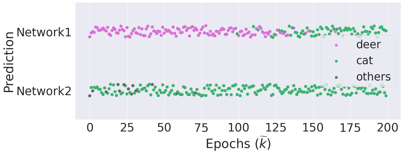
Figure 2: The evolution of output prediction of two neural networks during training on a single sample with a wrong randomly-assigned label (the assigned label is “cat” while the ground-truth label is “deer”) versus the number of epochs (steps) $\widetilde{k}$. Network1 is a GoogLeNet Szegedy et al. (2015) (pre-)trained on CIFAR-10 dataset with clean labels and has initial test accuracy of $95.36\%$. Network2 is a GoogLeNet (pre-)trained on CIFAR-10 dataset with $50\%$ label noise level and has initial test accuracy of $58.35\%$. Network2 has a lower test accuracy compared to Network1, and we observe that it memorizes this new sample after only $\widetilde{k}=2$ steps. In contrast, Network1 persists in predicting the correct output for this sample for longer and memorizes the new sample only after $\widetilde{k}=99$ steps. More examples and an ablation study on the effect of calibration are given in Figures 13 and 15 in Appendix D, respectively.

We perform the following empirical test. In Figure 2, we compare two deep neural networks. The first one has a high classification accuracy on unseen clean test data, whereas the other one has a low test accuracy. We then train both these models on a single sample with an incorrect label ($\widetilde{S}$ contains a single incorrectly-labeled sample). We observe that the model with a high test accuracy takes a long time (in terms of the number of training steps) to fit this sample; hence this model is resistant to memorization as the number of steps $\widetilde{k}$ required to fit $\widetilde{S}$ is large. In contrast, the model with a low test accuracy memorizes this sample after taking only a few steps; hence this model is susceptible to memorization as $\widetilde{k}$ required to fit $\widetilde{S}$ is small. This observation reinforces our intuition, that good models, measured by a high test accuracy, are more resistant to memorization of noisy labels.

Next, we further validate this observation theoretically by performing a convergence analysis on the held-out set $\widetilde{S}$, where the input samples $\{\widetilde{\textbf{x}}_{i}\}_{1}^{\widetilde{n}}$ of $\widetilde{S}$ are the same as the inputs of dataset $S$ (and hence $\widetilde{n}=n$). We consider the binary-classification setting. The output vector ${\widetilde{\textbf{y}}=\left(\widetilde{y}_{1},\cdots,\widetilde{y}_{n}\right)^{T}}$ is a vector of independent random labels that take values uniformly in $\{-1,1\}$. Therefore, creating this dataset $\widetilde{S}$ does not require extra information, and in particular no access to the data distribution $\mathcal{D}$. Consider the network $f_{\textbf{W}}(\textbf{x})$ as a two-layer neural network with ReLU non-linearity (denoted by ${\sigma(x)=\max\{x,0\}}$) and $m$ hidden-units:

$$f_{\textbf{W}}(\textbf{x})=\frac{1}{\sqrt{m}}\sum_{r=1}^{m}a_{r}\sigma\left(\textbf{w}_{r}^{T}\textbf{x}\right),$$

where $\textbf{x}\in\mathbb{R}^{d}$ is the input vector, $\textbf{W}=\left(\textbf{w}_{1},\cdots,\textbf{w}_{m}\right)\in\mathbb{R}^{d\times m}$, $\textbf{a}=\left(a_{1},\cdots,a_{m}\right)\in\mathbb{R}^{m}$ are the weight matrix of the first layer, and the weight vector of the second layer, respectively. For simplicity, the outputs associated with the input vectors $\{\textbf{x}_{i}\}_{1}^{n}$ are denoted by vector $\textbf{f}_{\textbf{W}}\in\mathbb{R}^{n}$ instead of $\{f_{\textbf{W}}(\textbf{x}_{i})\}_{1}^{n}$. The first layer weights are initialized as $\mathbf{w}_{r}(0)\sim\mathcal{N}\left(\textbf{0},\kappa^{2}\textbf{I}\right),\quad\forall r\in[m],$ where $0<\kappa\leq 1$ is the magnitude of initialization and $\mathcal{N}$ denotes the normal distribution. $a_{r}$s are independent random variables taking values uniformly in $\{-1,1\}$, and are considered to be fixed throughout training.

We define the objective function on datasets $S$ and $\widetilde{S}$, respectively, as

$$\Phi(\textbf{W})=\frac{1}{2}\left\lVert\textbf{f}_{\textbf{W}}-\textbf{y}\right\rVert_{2}^{2}=\frac{1}{2}\sum_{i=1}^{n}\left({f}_{\textbf{W}}(\textbf{x}_{i})-y_{i}\right)^{2},\quad\quad\widetilde{\Phi}(\textbf{W})=\frac{1}{2}\sum_{i=1}^{n}\left({f}_{\textbf{W}}(\textbf{x}_{i})-\widetilde{y}_{i}\right)^{2}.$$ (1)

Label noise level (LNL) of $S$ (and accordingly of the label vector y) is the ratio $n_{1}/n$, where $n_{1}$ is the number of samples in $S$ that have labels that are independently drawn uniformly in $\{-1,1\}$, and the remaining $n-n_{1}$ samples in $S$ have the ground-truth label. Hence, the two extremes are $S$ with LNL $=0$, which is the clean dataset, and $S$ with LNL $=1$, which is a dataset with entirely random labels.

To study the convergence of different models on $\widetilde{S}$, we compute the objective function $\widetilde{\Phi}(\textbf{W})$ after $\tilde{k}$ steps of training on the dataset $\widetilde{S}$. Therefore, the overall training/evaluation procedure is as follows; for $r\in[m]$, the second layer weights of the neural network are updated according to gradient descent:

$$\textbf{w}_{r}(t+1)-\textbf{w}_{r}(t)=-\eta\frac{\partial\overline{\Phi}\left(\textbf{W}(t)\right)}{\partial\textbf{w}_{r}},$$

where for $0\leq t<k$: $\overline{\Phi}=\Phi$, and for $k\leq t<k+\tilde{k}$: $\overline{\Phi}=\widetilde{\Phi}$, whereas $\eta$ is the learning rate. Note that we refer to $\Phi(\textbf{W}(t))$ as $\Phi(t)$ and to $\widetilde{\Phi}(\textbf{W}(t))$ as $\widetilde{\Phi}(t)$.

When a model fits the set $\widetilde{S}$, the value of $\widetilde{\Phi}$ becomes small, say below some threshold $\varepsilon$. The resistance of a model to memorization (fit) on the set $\widetilde{S}$ is then measured by the number of steps $\widetilde{k}^{*}(\varepsilon)$ such that $\widetilde{\Phi}(k+\widetilde{k})\leq\varepsilon$ for $\widetilde{k}>\widetilde{k}^{*}(\varepsilon)$. The larger (respectively, smaller) $\widetilde{k}^{*}$ is, the more the model is resistant (resp, susceptible) to this memorization. We can reason on the link between a good model and memorization from the following proposition.

Proposition 1 (Informal).

The objective function $\widetilde{\Phi}$ at step $k+\widetilde{k}$ is a decreasing function of the label noise level (LNL) in $S$, and of the number of steps $\widetilde{k}$.

Proposition 1 yields that models trained on $S$ with a low LNL (which are models with a high test accuracy on clean data) push $\widetilde{\Phi}(k+\widetilde{k})$ to become large. The number of steps $\widetilde{k}^{*}(\varepsilon)$ should therefore be large for $\widetilde{\Phi}$ to become less than $\epsilon$: these models resist the memorization of $\widetilde{S}$. Conversely, models trained on $S$ with a high LNL (which are models with a low test accuracy), allow for $\widetilde{k}^{*}(\varepsilon)$ to be small and give up rapidly to the memorization of $\widetilde{S}$. These conclusions match the empirical observation in Figure 2, and therefore further support the intuition that good models are resistant to memorization.

Refer to Section 5 for the formal theoretical results that produce Proposition 1.

3 Evaluating Resistance to Memorization

In Section 2 we showed that desirable models in terms of high classification accuracy on unseen clean data are resistant to the memorization of a randomly-labeled set. In this section, we describe a simple and computationally efficient metric to measure this resistance. To evaluate it efficiently at each step of the forward pass, we propose to take a single step on multiple randomly labeled samples, instead of taking multiple steps on a single randomly labeled sample (as done in Figure 2). To make the metric even more computationally efficient, instead of the entire randomly labeled set $\widetilde{S}$ (as in our theoretical developments), we only take a single mini-batch of $\widetilde{S}$. For simplicity and with some abuse of notation, we still refer to this single mini-batch as $\widetilde{S}$.

Algorithm 1 Computes the susceptibility to noisy labels $\zeta$

1:  Input: Dataset $S$, Number of Epochs $T$

2:  Sample a mini-batch $\widetilde{S}$ from $S$; Replace its labels with random labels

3:  Initialize network $f_{\textbf{W}(0)}$

4:  Initialize $\zeta(0)=0$

5:  for $t=1,\cdots,T$ do

6:     Update $f_{\textbf{W}(t)}$ from $f_{\textbf{W}(t-1)}$ using dataset $S$

7:     Compute $\widetilde{\Phi}(\textbf{W}(t))$

8:     Update $f_{\widetilde{\textbf{W}}(t+1)}$ from $f_{\textbf{W}(t)}$ using dataset $\widetilde{S}$

9:     Compute $\widetilde{\Phi}(\widetilde{\textbf{W}}(t+1))$

10:     Compute $\zeta(t)=\frac{1}{t}\Big{[}(t-1)\zeta(t-1)\allowbreak+\widetilde{\Phi}(\textbf{W}(t))-\widetilde{\Phi}(\widetilde{\textbf{W}}(t+1))\Big{]}$

11:  end for

12:  Return $\zeta$.

To track the prediction of the model over multiple samples, we compare the objective function ($\widetilde{\Phi}$) on $\widetilde{S}$ before and after taking a single optimization step on it. The learning rate, and its schedule, have a direct effect on this single optimization step. For certain learning rate schedules, the learning rate might become close to zero (e.g., at the end of training), and hence the magnitude of this single step would become too small to be informative. To avoid this, and to account for the entire history of the optimization trajectory, we compute the average difference over the learning trajectory (a moving average). We propose the following metric, which we call susceptibility to noisy labels, $\zeta(t)$. At step $t$ of training,

$$\zeta(t)=\frac{1}{t}\sum_{\tau=1}^{t}\left[\widetilde{\Phi}\left(\textbf{W}(\tau)\right)-\widetilde{\Phi}\left(\widetilde{\textbf{W}}\left(\tau+1\right)\right)\right]\;,$$ (2)

where ${\textbf{W}}\left(\tau\right)$, $\widetilde{\textbf{W}}\left(\tau+1\right)$ are the model parameters before and after a single update step on $\widetilde{S}$. Algorithm 1 describes the computation of $\zeta$. The lower $\zeta(t)$ is, the less the model changes its predictions for $\widetilde{S}$ after a single step of training on it, and thus the less it memorizes the randomly-labeled samples. We say therefore that a model is resistant (to the memorization of randomly-labeled samples) when the susceptibility to noisy labels $\zeta(t)$ is low.

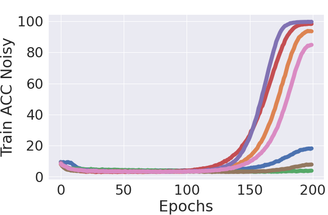
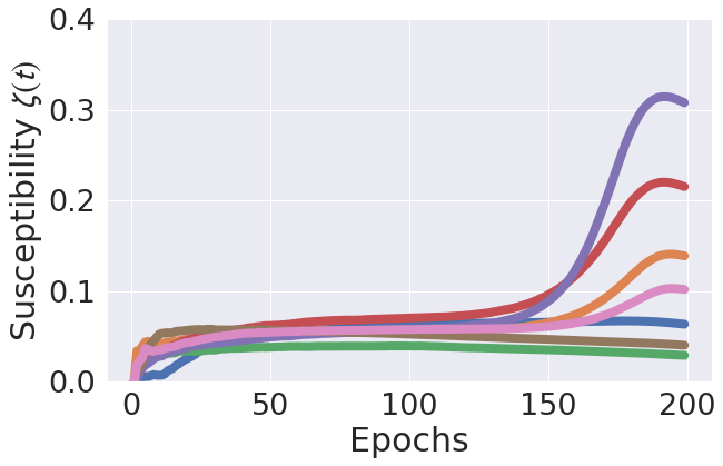
Figure 3: Accuracy on the noisy subset of the training set versus susceptibility $\zeta(t)$ (Equation (2)) for deep convolutional neural networks (ranging from a $5-$layer cnn to more sophisticated structures such as EfficientNet Tan and Le (2019)) trained on CIFAR-10 with $50\%$ label noise. We observe a strong Pearson correlation coefficient between Train ACC Noisy and $\zeta(t)$: $\rho=0.884$.

Susceptibility $\zeta$ tracks memorization for different models

The classification accuracy of a model on a set is defined as the ratio of the number of samples where the label predicted by the model matches the label on the dataset, to the total number of samples. We refer to the subset for which the dataset label is different from the ground-truth label as the noisy subset of the training set. Its identification requires access to the ground-truth label. Recall that we refer to memorization within the training set as the fit on the noisy subset, which is measured by the accuracy on it. We call this accuracy “Train ACC Noisy” in short. In Figure 3, we observe a strong positive correlation between the memorization of the held-out randomly labeled set, which is tracked by $\zeta(t)$ (Equation (2)) and the memorization of noisy labels within the training set, tracked by Train ACC Noisy. Susceptibility $\zeta$, which is computed on a mini-batch with labels independent from the training set, can therefore predict the resistance to memorization of the noisy subset of the training set. In Figure 34, we show the robustness of susceptibility $\zeta$ to the mini-batch size, and to the choice of the particular mini-batch.

Susceptibility $\zeta$ tracks memorization for a single model

It is customary when investigating different capabilities of a model, to keep checkpoints/snapshots during training and decide which one to use based on the desired property, see for example (Zhang et al., 2019a; Chatterji et al., 2019; Neyshabur et al., 2020; Andreassen et al., 2021; Baldock et al., 2021). With access to ground-truth labels, one can track the fit on the noisy subset of the training set to find the model checkpoint with the least memorization, which is not necessarily the end checkpoint, and hence an early-stopped version of the model. However, the ground-truth label is not accessible in practice, and therefore the signals presented in Figure 3 (left) are absent. Moreover, as discussed in Figure 8, the training accuracy on the entire training set is also not able to recover these signals. Using susceptibility $\zeta$, we observe that these signals can be recovered without any ground-truth label access, as shown in Figure 3 (right). Therefore, $\zeta$ can be used to find the model checkpoint with the least memorization. For example, in Figure 3, for the ResNet model, susceptibility $\zeta$ suggests to select model checkpoints before it sharply increases, which exactly matches with the sharp increase in the fit on the noisy subset. On the other hand, for the EfficientNet model, susceptibility suggests to select the end checkpoint, which is also consistent with the selection according to the fit on the noisy subset.

4 Good Models are Resistant and Trainable

When networks are trained on a dataset that contains clean and noisy labels, the fit on the clean and noisy subsets affect the generalization performance of the model differently. Therefore, as we observe in Figure 4a for models trained on a noisy dataset (details are deferred to Appendix B), the correlation between the training accuracy (accuracy on the entire training set) and the test accuracy (accuracy on the unseen clean test set) is low. Interestingly however, we observe in Figure 4b that if we remove models with a high memorization on the noisy subset, as indicated by a large susceptibility to noisy labels $\zeta(t)$, then the correlation between the training and the test accuracies increases significantly (from $\rho=0.608$ to $\rho=0.951$), and the remaining models with low values of $\zeta(t)$ have a good generalization performance: a higher training accuracy implies a higher test accuracy. This is especially important in the practical settings where we do not know how noisy the training set is, and yet must reach a high accuracy on clean test data.

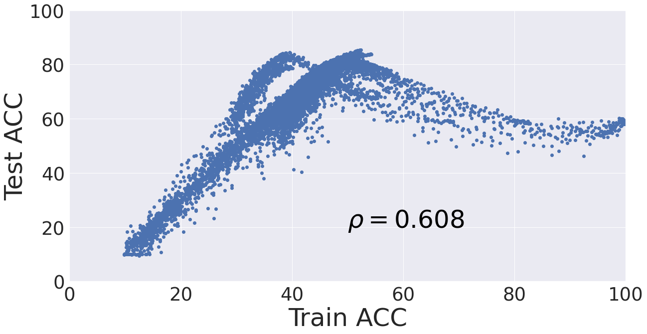
(a)

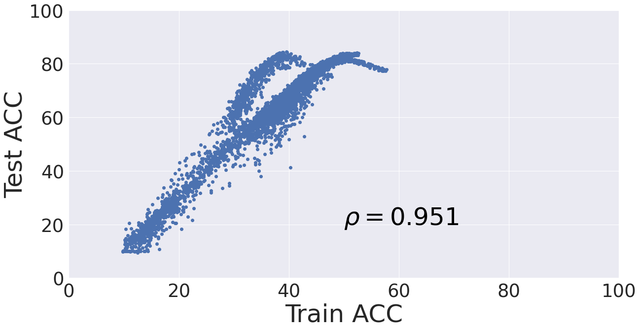
(b)

Figure 4: The effect of filtering the models based on the susceptibility metric $\zeta(t)$ for models trained on CIFAR-10 with $50\%$ label noise. We observe that by removing models with a high value of $\zeta(t)$, the correlation between the training accuracy (accessible to us in practice) and the test accuracy (not accessible) increases a lot, and we observe that among the selected models, a higher training accuracy implies a higher test accuracy. Refer to Figures 17, 19, 22, 25, 27 for similar results on $5$ other datasets. We use a threshold such that half of the models have $\zeta$ < threshold and hence remain after filtration.

After removing models with large values of $\zeta(t)$, we select models with a low label noise memorization. However, consider an extreme case: a model that always outputs a constant is also low at label noise memorization, but does not learn the useful information present in the clean subset of the training set either. Clearly, the models should be “trainable” on top of being resistant to memorization. A “trainable model" is a model that has left the very initial stages of training, and has enough capacity to learn the information present in the clean subset of the dataset to reach a high accuracy on it. The training accuracy on the entire set is a weighted average of the training accuracy on the clean and noisy subsets. Therefore, among the models with a low accuracy on the noisy subset (selected using susceptibility $\zeta$ in Figure 4b), we should further restrict the selection to those with a high overall training accuracy, which corresponds to a high accuracy on the clean subset.

We can use the two metrics, susceptibility to noisy labels $\zeta(t)$ and overall training accuracy, to partition models that are being trained on some noisy dataset in different regions. For simplicity, we use the average values of $\zeta$ and training accuracy as thresholds that are used to obtain four different regions. In Appendix F and Figure 37, we observe that our model selection approach is robust to this threshold choice. According to this partitioning and as shown in Figure 6 the models in each region are: Region 1: Trainable and resistant to memorization (i.e., having a high training accuracy and a low $\zeta$), Region 2: Trainable but not resistant, Region 3: Not trainable but resistant, and Region 4: Neither trainable nor resistant. Note that the colors of each point, which indicate the value of the test accuracy are only for illustration and are not used to find these regions. The average test accuracy is the highest for models in Region 1 (i.e., that are resistant to memorization on top of being trainable). In particular, going from Region 2 to Region 1 increases the average test accuracy of the selected models from $70.59\%$ to $76\%$, i.e., a $7.66\%$ relative improvement in the test accuracy. This improvement is consistent with other datasets as well: $6.7\%$ for Clothing-1M (Figure LABEL:fig:mainclothing1m), $4.2\%$ for Animal-10N (Figure LABEL:fig:mainanimal10n), $2.06\%$ for CIFAR-10N (Figure LABEL:fig:maincifar10n), $31.4\%$ for noisy MNIST (Figure 16), $33\%$ for noisy Fashion-MNIST (Figure 18), $33.6\%$ for noisy SVHN (Figure 20), $15.1\%$ for noisy CIFAR-100 (Figure 23), and $8\%$ for noisy Tiny ImageNet (Figure 26) datasets (refer to Appendix E for detailed results).

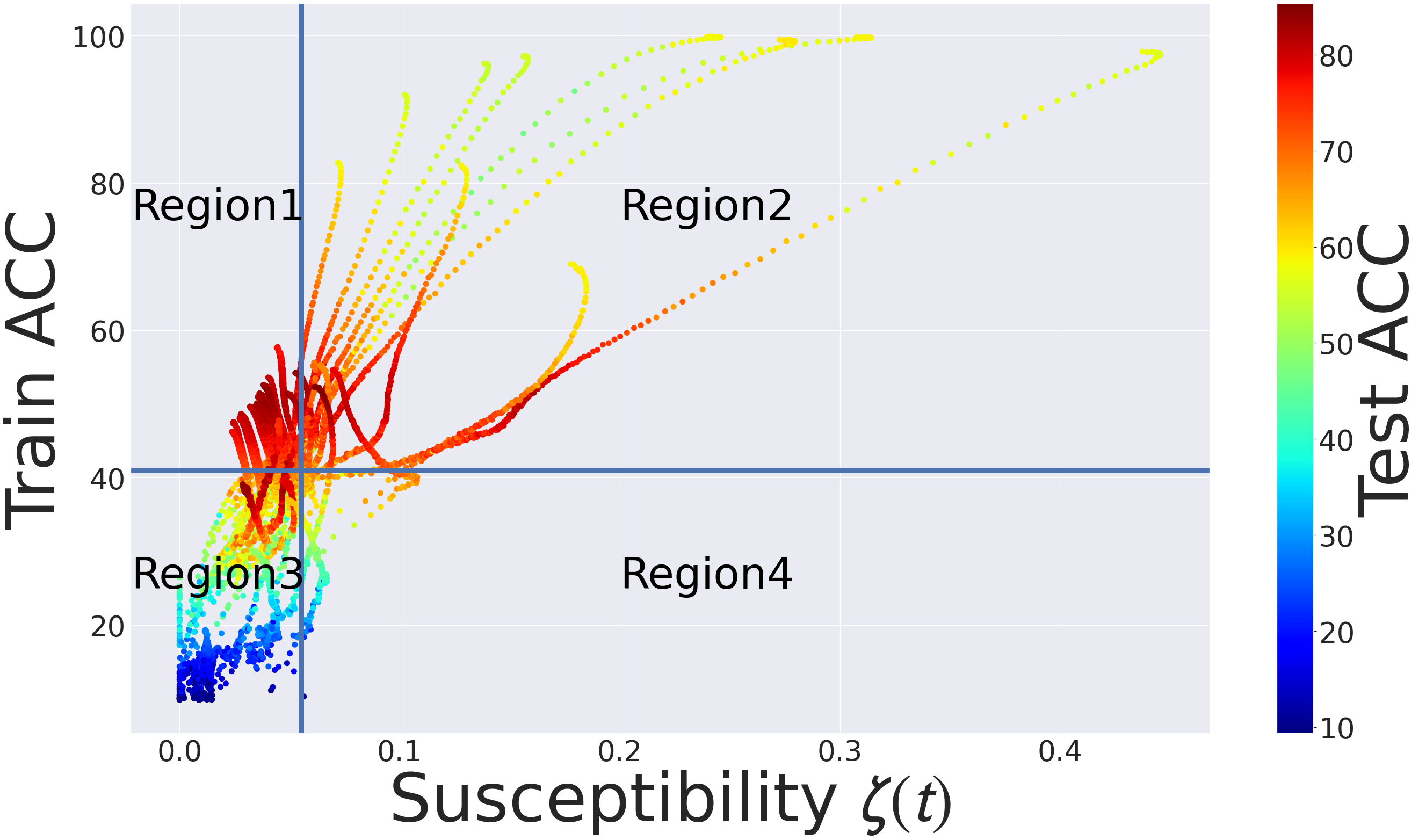
Figure 5: For models trained on CIFAR-10 with $50\%$ label noise, we use two thresholds on susceptibility and accuracy to divide these models into 4 regions and corresponding categories as follows. We use the average values of $\zeta(t)$ and of the training accuracy over the available models as the thresholds. Region  1: Trainable and resistant, with average test accuracy of $\mathbf{76}\%$. Region 2: Trainable and but not resistant, with average test accuracy of $70.59\%$. Region 3: Not trainable but resistant, with average test accuracy of $52.49\%$. Region 4: Neither trainable nor resistant, with average test accuracy of $58.23\%$. We observe that the models in Region 1 generalize well on unseen data, as they have a high test accuracy.

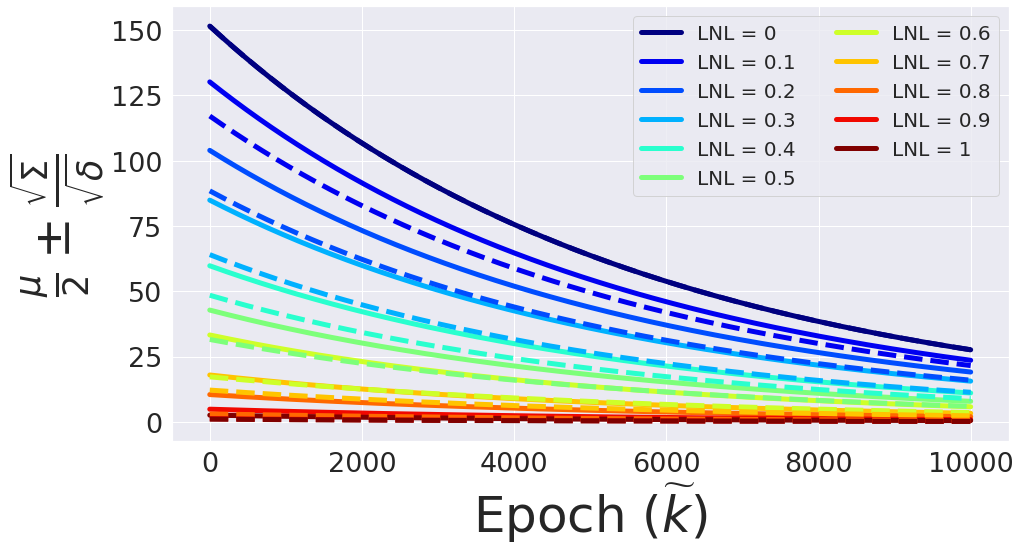
Figure 6: The lower (dashed lines) and upper (solid lines) bound terms of Theorem 2 that depend on the label noise level (LNL). They are computed from the eigenvectors and eigenvalues of the Gram-matrix for $1000$ samples of the MNIST dataset, computed over $10$ random draws computed with hyper-parameters $\eta=10^{-6}$, $k=10000$ and $\delta=0.05$. We observe that both the lower and the upper bounds in Theorem 2 are a decreasing function of LNL and of the number of epochs $\tilde{k}$. Therefore, we conclude that $\widetilde{\Phi}(k+\tilde{k})$ is also a decreasing function of LNL and of $\tilde{k}$ (Proposition 1).

Comparison with using a noisy validation set:

Given a dataset containing noisy labels, a correctly-labeled validation set is not accessible without ground-truth label access. One can however use a subset of the available dataset and assess models using this noisy validation set. An important advantage of our approach compared to this assessment is the information that it provides about the memorization within the training set, which is absent from performance on a test set or a noisy validation set. For example, in Figures 32a and 33a we observe models (on the very top right) that have memorized $100\%$ of the noisy subset of the training set, and yet have a high test accuracy. However, some models (on the top middle/left part of the figure), which have the same fit on the clean subset but lower memorization, have lower or similar test accuracy. For more details, refer to Appendix C.

Moreover, as formally discussed in (Lam and Stork, 2003), the number of noisy validation samples that are equivalent to a single clean validation sample depends on the label noise level of the dataset and on the true error rate of the model, which are both unknown in practice, making it difficult to pick an acceptable size for the validation set without compromising the training set. If we use a small validation set (which allows for a large training set size), then we observe a very low correlation between the validation and the test accuracies (as reported in Table 1 and Figure 12 in Appendix C). In contrast, our approach provides much higher correlation to the test accuracy. We also conducted experiments with noisy validation sets with larger sizes and observed that the size of the noisy validation set would need to be increased around ten-fold to reach the same correlation as our approach. Increasing the size of the validation set removes data out of the training set, which may degrade the overall performance, whereas our approach leaves the entire available dataset for training. Overall, in addition to robustness against label noise level and dataset size, our approach brings advantages in offering a gauge on memorization, without needing extra data, while maintaining a very low computational cost.

5 Convergence Analysis

In this section, we elaborate on the analysis that leads to (the informal) Proposition 1. A matrix, a vector, and a scalar are denoted respectively by $\textbf{A},\textbf{a}$, and $a$. The identity matrix is denoted by I. The indicator function of a random event $A$ is denoted by $\mathbb{I}(A)$. The $(i,j)-$th entry of Matrix A is $\textbf{A}_{ij}$.

Consider the setting described in Section 2 with $\left\lVert\mathbf{x}\right\rVert_{2}=1$ and $\left\lvert y\right\rvert\leq 1$ for $(\mathbf{x},y)\sim\mathcal{D}\coloneqq\mathcal{X}\times\mathcal{Y}$, where $\mathcal{X}=\mathbb{R}^{d}$ and $\mathcal{Y}=\mathbb{R}$. For input samples $\{\textbf{x}_{i}\}_{1}^{n}$, the $n\times n$ Gram matrix $\textbf{H}^{\infty}$ has entries

$$\textbf{H}_{ij}^{\infty}=\mathbb{E}_{\textbf{w}\sim\mathcal{N}(\textbf{0},\textbf{I})}\left[\textbf{x}_{i}^{T}\textbf{x}_{j}\mathbb{I}\{\textbf{w}^{T}\textbf{x}_{i}\geq 0,\textbf{w}^{T}\textbf{x}_{j}\geq 0\}\right]=\frac{\textbf{x}_{i}^{T}\textbf{x}_{j}\left(\pi-\arccos(\textbf{x}_{i}^{T}\textbf{x}_{j})\right)}{2\pi},\;\forall i,j\in[n],$$ (3)

and its eigen-decomposition is $\textbf{H}^{\infty}=\sum_{i=1}^{n}\lambda_{i}\textbf{v}_{i}\textbf{v}_{i}^{T}$, where the eigenvectors ${\textbf{v}_{i}\in\mathbb{R}^{n}}$ are orthonormal and $\lambda_{0}=\min\{\lambda_{i}\}_{1}^{n}$. Using the eigenvectors and eigenvalues of $\textbf{H}^{\infty}$, we have the following theorem.

Theorem 1.

For $\kappa=O\left(\frac{\epsilon\sqrt{\delta}\lambda_{0}}{n^{3/2}}\right)$, $m=\Omega\left(\frac{n^{9}}{\lambda_{0}^{6}\epsilon^{2}\kappa^{2}\delta^{4}}\right)$, and $\eta=O\left(\frac{\lambda_{0}}{n^{2}}\right)$, with probability at least $1-\delta$ over the random parameter initialization described in Section 2 , we have:

$$\left\lVert\textbf{f}_{\textbf{W}(k+\tilde{k})}-\widetilde{\textbf{y}}\right\rVert_{2}=\sqrt{\sum_{i=1}^{n}\left[\textbf{v}_{i}^{T}\textbf{y}-\textbf{v}_{i}^{T}\widetilde{\textbf{y}}-\left(1-\eta\lambda_{i}\right)^{k}\textbf{v}_{i}^{T}\textbf{y}\right]^{2}(1-\eta\lambda_{i})^{2\tilde{k}}}\pm\epsilon.$$

The proof is provided in Appendix J.

Theorem 1 enables us to approximate the objective function on dataset $\widetilde{S}$ (Equation (1)) as follows:

$$\widetilde{\Phi}(k+\tilde{k})\approx\frac{1}{2}\sum_{i=1}^{n}\left[p_{i}-\widetilde{p}_{i}-\left(1-\eta\lambda_{i}\right)^{k}p_{i}\right]^{2}(1-\eta\lambda_{i})^{2\tilde{k}}\;,$$ (4)

where $p_{i}=\textbf{v}_{i}^{T}\textbf{y}$ and $\widetilde{p}_{i}=\textbf{v}_{i}^{T}\widetilde{\textbf{y}}$. Let us define

$$\mu=\sum_{i=1}^{n}\mathbb{E}\left[p_{i}^{2}\right]\left[1-\left(1-\eta\lambda_{i}\right)^{k}\right]^{2}\left(1-\eta\lambda_{i}\right)^{2\tilde{k}},\quad\Sigma=\text{Var}_{\widetilde{\textbf{p}},\textbf{p}}\left[\widetilde{\Phi}(k+\tilde{k})\right].$$ (5)

We numerically observe that $\mu/2\pm\sqrt{\Sigma/\delta}$ are both decreasing functions of the label noise level (LNL) of the label vector y, and of $\widetilde{k}$ (see Figures 6, and 38, 39, 40, 41 in Appendix K for different values of the learning rate $\eta$, number of steps $k$, and datasets). The approximation in Equation (4) together with the above observation then yields the following lower and upper bounds for $\widetilde{\Phi}(k+\tilde{k})$.

Theorem 2.

With probability at least $1-\delta$ over the draw of the random label vector $\widetilde{\textnormal{{y}}}$, given the approximation made in Equation (4),

$$\frac{\mu}{2}-\sqrt{\frac{\Sigma}{\delta}}\leq\widetilde{\Phi}(k+\tilde{k})-\frac{1}{2}\sum_{i=1}^{n}\left(1-\eta\lambda_{i}\right)^{2\tilde{k}}\leq\frac{\mu}{2}+\sqrt{\frac{\Sigma}{\delta}}\;$$ (6)

The proof is provided in Appendix K. Because the term $\sum_{i=1}^{n}\left(1-\eta\lambda_{i}\right)^{2\tilde{k}}$ is independent of LNL of the label vector y, we can conclude that $\widetilde{\Phi}(k+\tilde{k})$ is a decreasing function of LNL. Moreover, Since $0<1-\eta\lambda_{i}<1$, the term $\sum_{i=1}^{n}\left(1-\eta\lambda_{i}\right)^{2\tilde{k}}$ is also a decreasing function of $\widetilde{k}$. Therefore, similarly, we can conclude that $\widetilde{\Phi}(k+\tilde{k})$ is a decreasing function of $\widetilde{k}$. Proposition 1 summarizes this result.

6 Experiments on Real-world Datasets with noisy labels

To evaluate the performance of our approach on real-world datasets, we have conducted additional experiments on the Clothing-1M dataset Xiao et al. (2015), which is a dataset with $1$M images of clothes, on the Animal-10N dataset (Song et al., 2019), which is a dataset with $50$k images of animals and on the CIFAR-10N dataset (Wei et al., 2022), which is the CIFAR-10 dataset with human-annotated noisy labels obtained from Amazon Mechanical Turk. In the Clothing-1M dataset, the images have been labeled from the texts that accompany them, hence there are both clean and noisy labels in the set, and in the Animal-10N dataset, the images have been gathered and labeled from search engines. In these datasets, some images have incorrect labels and the ground-truth labels in the training set are not available. Hence in our experiments, we cannot explicitly track memorization as measured by the accuracy on the noisy subset of the training set.

We train different settings on these two datasets with various architectures (including ResNet, AlexNet and VGG) and varying hyper-parameters (refer to Appendix B for details). We compute the training accuracy and susceptibility $\zeta$ during the training process for each setting and visualize the results in Figure 7 (a)-(c).

Computation   
Selection   
Evaluation

(a)

(b)

(c)

(d)

(e)

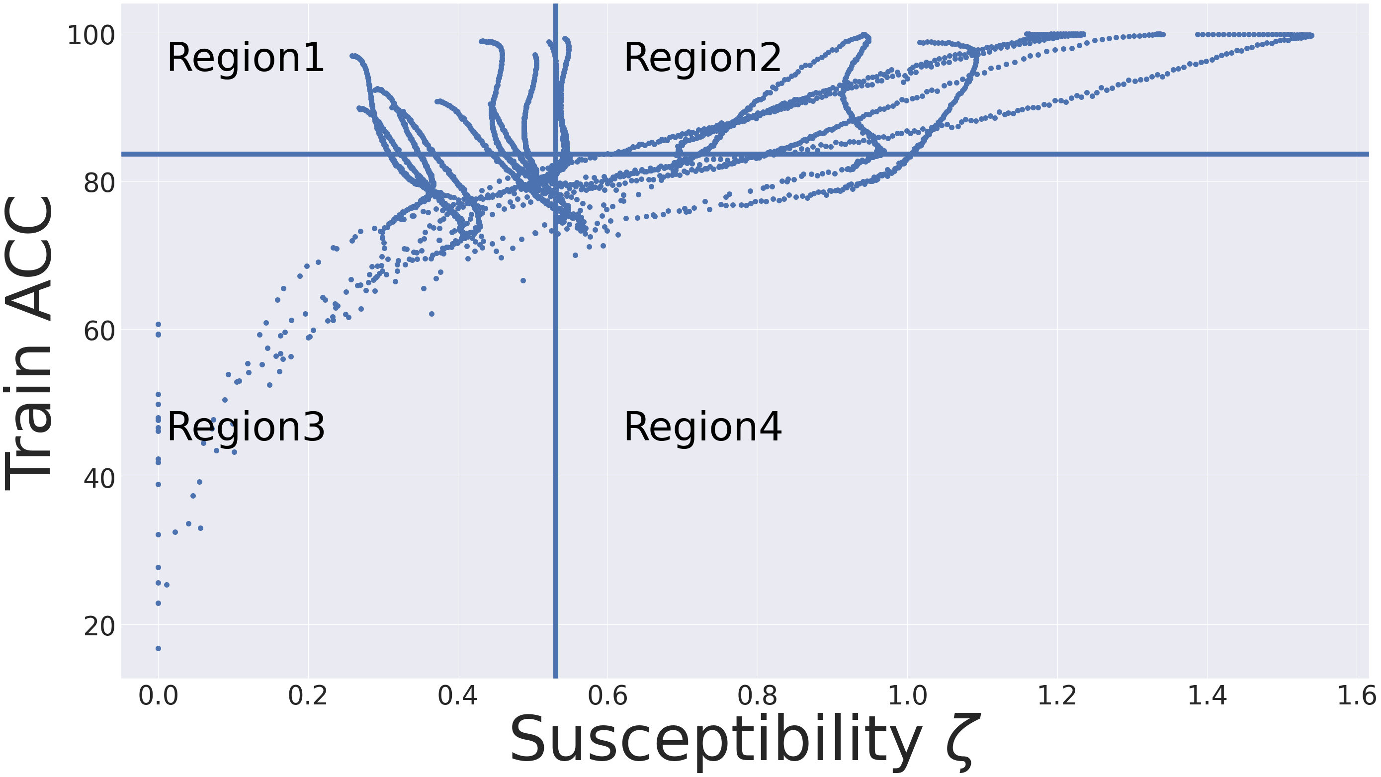
(f)

(g)

(h)

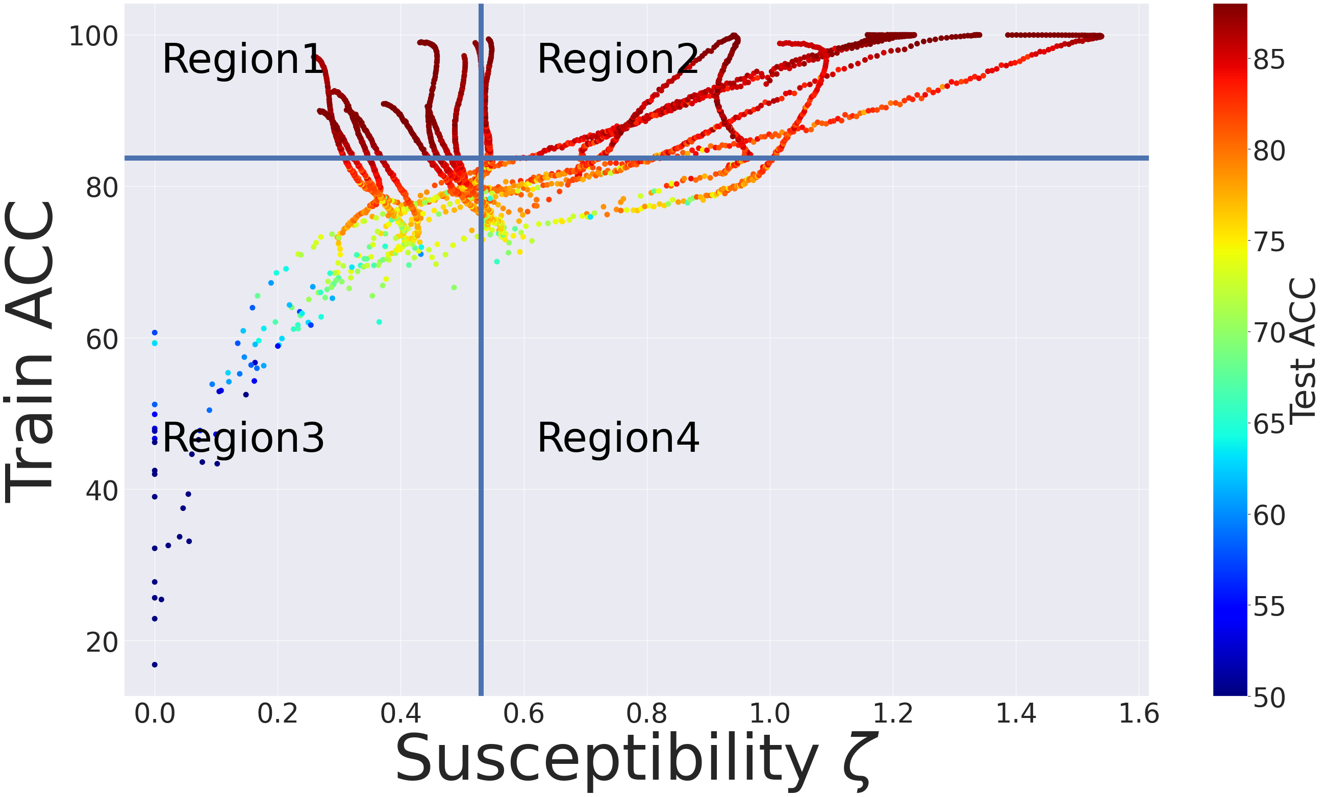
(i)

Figure 7: For real-world noisy labeled datasets, we show in three steps the efficiency of our model-selection approach. Top: Training accuracy and susceptibility $\zeta$ are computed for models trained on each dataset. Middle: According to the average values of the training accuracy and susceptibility $\zeta$ the figure is divided into $4$ regions. Our model-selection approach suggests selecting models in Region 1, which are resistant to memorization on top of being trainable. Bottom: The test accuracy of the models is visualized using the color of each point (which is only for illustration and is not used to find different regions). We can observe that models in Region 1 have the highest test accuracies in each dataset.

We divide the models of Figure 7 (a)-(c) into 4 regions, where the boundaries are set to the average value of the training accuracy (horizontal line) and the average value of susceptibility (vertical line): Region 1: Models that are trainable and resistant to memorization, Region 2: Trainable and but not resistant, Region 3: Not trainable but resistant and Region 4: Neither trainable nor resistant. This is shown in Figure 7 (d)-(f).

Our approach suggests selecting models in Region 1 (low susceptibility, high training accuracy). In order to assess how our approach does in model selection, we can reveal the test accuracy computed on a held-out clean test set in Figure 7 (g)-(i). We observe that the average (± standard deviation) of the test accuracy of models in each region is as follows:

• Clothing-1M dataset: Region 1: 61.799$\%$ ± 1.643; Region 2: 57.893$\%$ ± 3.562; Region 3: 51.250$\%$ ± 17.209; Region 4: 51.415$\%$ ± 9.709.

• Animal-10N dataset: Region 1: 96.371$\%$ ± 1.649; Region 2: 92.508$\%$ ± 2.185; Region 3: 91.179$\%$ ± 6.601; Region 4: 89.352$\%$ ± 3.142.

• CIFAR-10N dataset: Region 1: 87.2$\%$ ± 0.99; Region 2: $85.44\%$ ± 2.52; Region 3: 77.87$\%$ ± 8.15; Region 4: 78.45$\%$ ± 3.86.

We observe that using our approach we are able to select models with very high test accuracy. In addition, the test accuracies of models in Region 1 have the least amount of standard deviation. Note that our susceptibility metric $\zeta$ does not use any information about the label noise level or the label noise type that is present in these datasets. Similarly to the rest of this paper, random labeling is used for computing $\zeta$. Interestingly, even though within the training sets of these datasets the label noise type is different than random labeling (label noise type is instance-dependent Xia et al. (2020); Wei et al. (2022)), $\zeta$ is still successfully tracking memorization.

Therefore, our approach selects trainable models with low memorization even for datasets with real-world label noise. Observe that selecting models only on the basis of their training accuracy or only on the basis of their susceptibility fails: both are needed. It is interesting to note that in the Clothing-1M dataset, as the dataset is more complex, the range of the performance of different models varies and our approach is able to select “good” models from “bad” models. On the other hand, in the Animal-10N dataset, as the dataset is easier to learn and the estimated label noise level is lower, most models are already performing rather well. Here, our approach is able to select the “best” models from “good” models.

7 On the Generality of the Observed Phenomena

In this section, we provide additional experiments that show our empirical results hold across different choices of dataset, training, and architecture design as well as label noise level and form.

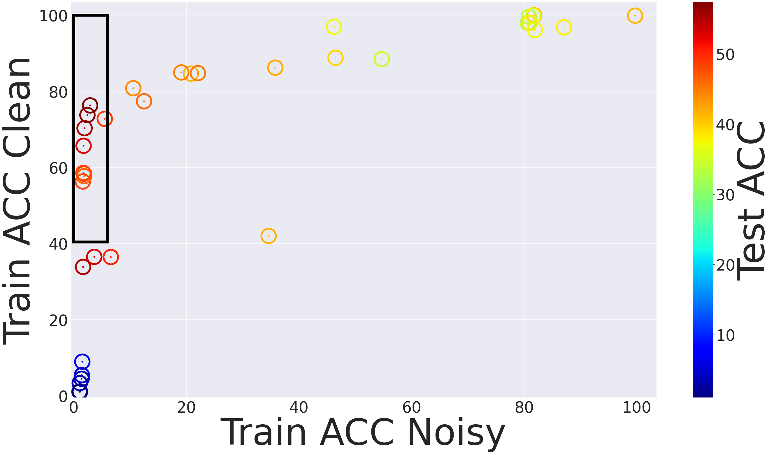
(a) With oracle access to the ground-truth label.
Average test accuracy of the selected models = $51.39\%$

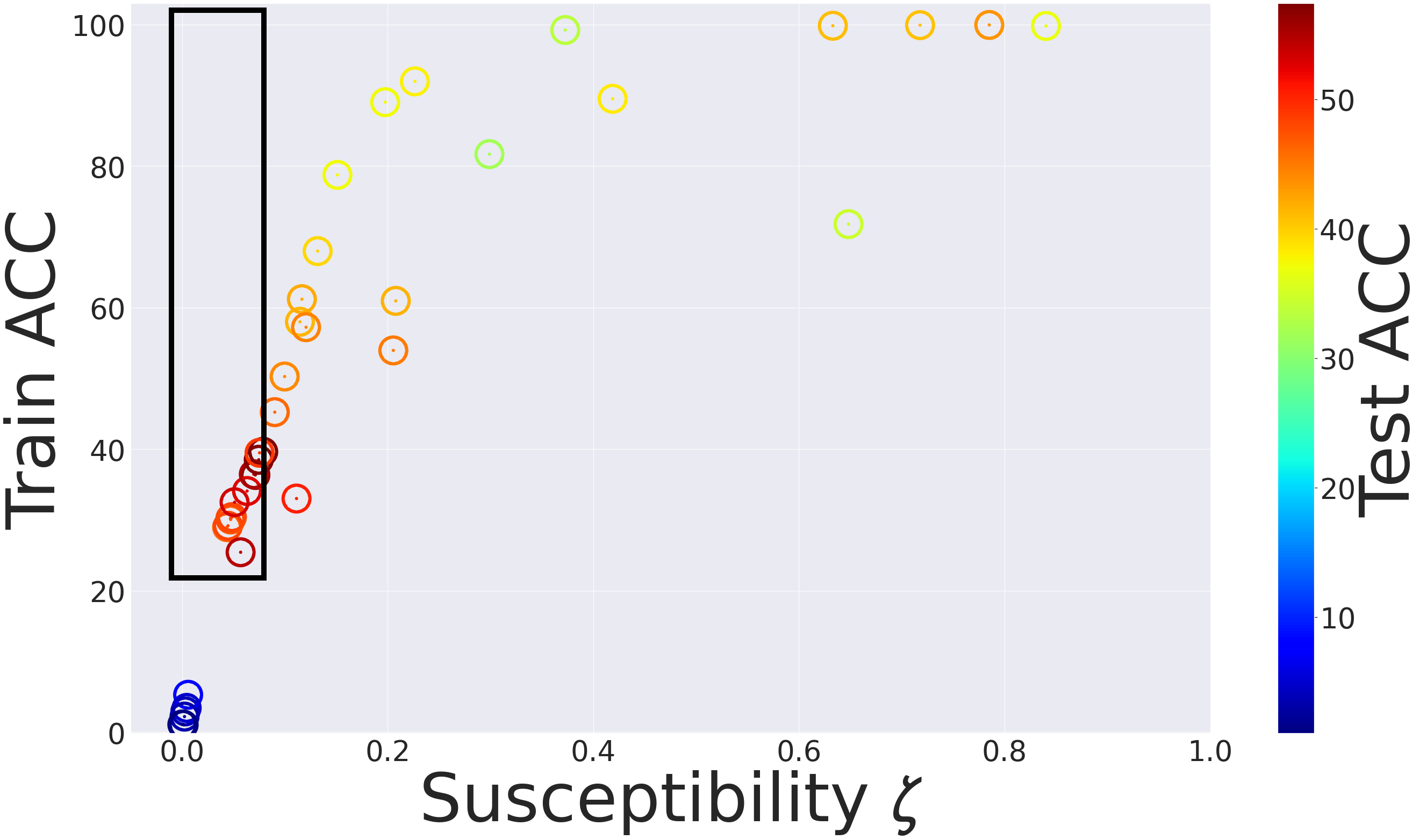
(b) Without access to the ground-truth label.
Average test accuracy of the selected models = $49.57\%$

Figure 24: For models trained on CIFAR-100 with $50\%$ label noise, with the help of our susceptibility metric $\zeta(t)$ and the overall training accuracy, we can recover models with a high/low accuracy on the clean/noisy subset.

Dataset: In addition to the real-world datasets provided in the previous section, our results consistently hold for datasets MNIST, Fashion MNIST, SVHN, CIFAR-100, and Tiny ImageNet datasets; see Figures 16-27 in Appendix E.

Learning rate schedule: Our results are not limited to a specific optimization scheme. In our experiments, we apply different learning rate schedules, momentum values, and optimizers (SGD and Adam) (for details see Appendix B). More specifically, we show in Figure 29 (in Appendix F) that the strong correlation between memorization and our metric $\zeta(t)$ stays consistent for both learning rate schedulers cosineannealing and exponential.

Architecture: Results of Sections 3 and 4 are obtained from a variety of architecture families, such as DenseNet Huang et al. (2017), MobileNet Howard et al. (2017), VGG Simonyan and Zisserman (2014), and ResNet He et al. (2016a). For the complete list of architectures, see Appendix B. We observe that $\zeta(t)$ does not only detect resistant architecture families (as done for example in Figure 3), but that it is also able to find the best design choice (e.g., width) among configurations that are already resistant, see Figure 28 in Appendix F.

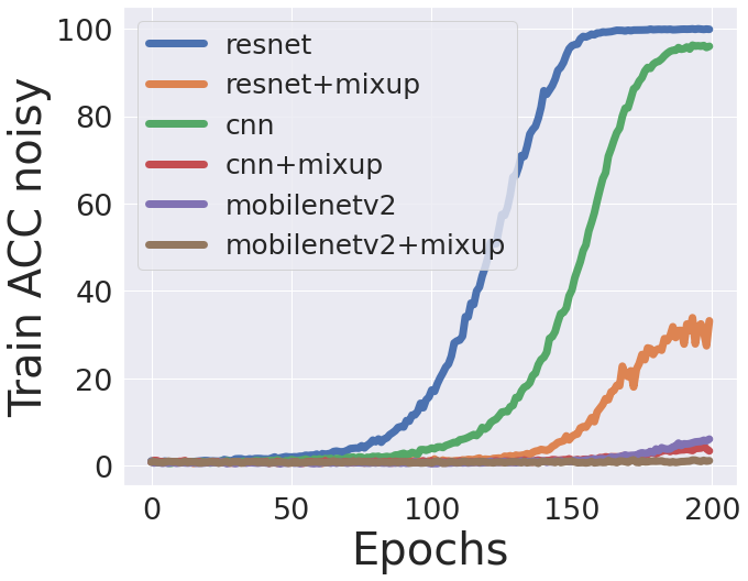
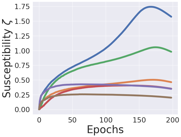
Figure 31: Accuracy on the noisy subset of the training set versus susceptibility to noisy labels $\zeta(t)$ for networks trained on CIFAR-100 with $10\%$ label noise. Pearson correlation between Train ACC Noisy and $\zeta$ is $\rho=0.849$.

Low label noise levels: In addition to the real-world datasets with low label noise levels (label noise level of Animal-10N and CIFAR-10N are $8\%$ and $9\%$, respectively), we studied low label noise levels in datasets with synthetic label noises as well. For models trained on CIFAR-10 and CIFAR-100 datasets with $10\%$ label noise (instead of $50\%$), we still observe a high correlation between accuracy on the noisy subset and $\zeta(t)$ in Figures 30 and 31 in Appendix F. Moreover, we observe in Figures 32 and 33 in Appendix F that the average test accuracy of the selected models using our metric is comparable with the average test accuracy of the selected models with access to the ground-truth label.

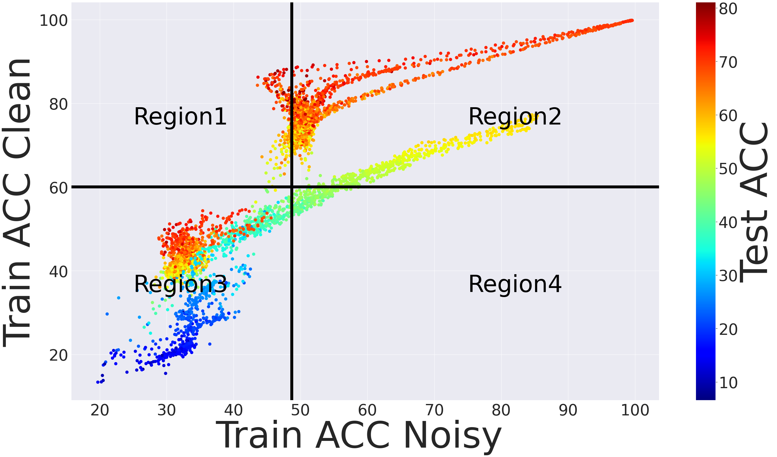
(a) With access to the ground-truth label.
Average test accuracy of the selected models = $66.793\%$

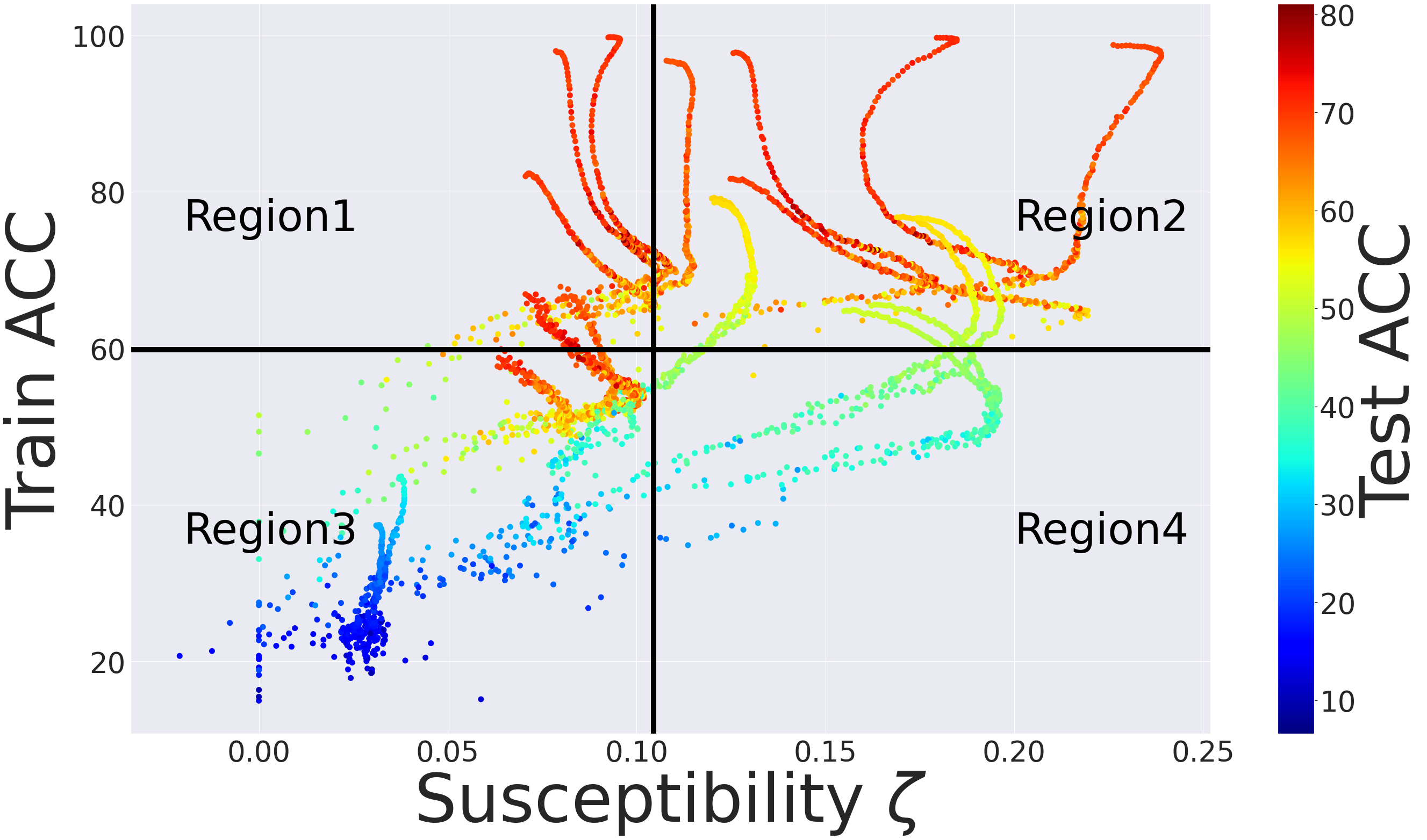
(b) Without access to the ground-truth label. Average test accuracy of the selected models = $66.307\%$

Figure 36: For models trained for $200$ epochs on CIFAR-10 with $50\%$ asymmetric label noise as proposed in Xia et al. [2021], using susceptibility $\zeta$ and the overall training accuracy, the average test accuracy of the selected models is comparable with the case of having access to the ground-truth label.

Asymmetric label noise: In addition to the real-world datasets with asymmetric label noises (label noise type of the datasets in Section 6 is instance-dependent Xia et al. (2020); Wei et al. (2022)), we studied synthetic asymmetric label noise as well. We have performed experiments with asymmetric label noise as proposed in (Xia et al., 2021). Using our approach, the average test accuracy of the selected models is $66.307\%$, whereas the result from oracle is $66.793\%$ (see Figure 36 in Appendix E).

8 Conclusion

We have proposed a simple but surprisingly effective approach to track memorization of the noisy subset of the training set using a single mini-batch of unlabeled data. Our contributions are three-fold. First, we have shown that models with a high test accuracy are resistant to memorization of a held-out randomly-labeled set. Second, we have proposed a metric, susceptibility, to efficiently measure this resistance. Third, we have empirically shown that one can utilize susceptibility and the overall training accuracy to distinguish models (whether they are a single model at various checkpoints, or different models) that maintain a low memorization on the training set and generalize well to unseen clean data while bypassing the need to access the ground-truth label. We have studied model selection in a variety of experimental settings and datasets with label noise, ranging from selecting the “best” models from “good” models (for easy datasets such as Animal-10N) to selecting “good” models from “bad” models (for more complex datasets such as Clothing-1M).

Our theoretical results have direct implications for online settings. When the quality of the labels for new data stream is low, Theorem 1 can directly compare how different models converge on this low-quality data, and help in selecting resistant models, which converge slowly on this data. Our empirical results provide new insights on the way models memorize the noisy subset of the training set: the process is similar to the memorization of a purely randomly-labeled held-out set.

Acknowledgement

We thank Chiyuan Zhang and Behnam Neyshabur for their valuable feedback on the draft of this work.

Appendix A Additional Related Work

Memorization

Arpit et al. [2017] describe memorization as the behavior shown by neural networks when trained on noisy data. Patel and Sastry [2021] define memorization as the difference in the predictive performance of models trained on clean data and on noisy data distributions, and propose a robust objective function that resists to memorization. The effect of neural network architecture on their robustness to noisy labels is studied in Li et al. [2021], which measures robustness to noisy labels by the prediction performance of the learned representations on the ground-truth target function. Feldman and Zhang [2020] formally define memorization of a sample for an algorithm as the inability of the model to predict the output of a sample based on the rest of the dataset, so that the only way that the model can fit the sample is by memorizing its label. Our definition of memorization as the fit on the noisy subset of the training set follows the same principle; the fit of a randomly-labeled individual sample is only possible if the totally random label associated with the sample is memorized, and it is impossible to predict using the rest of the dataset.

Learning before Memorization

Multiple studies have reported that neural networks learn simple patterns first, and memorize the noisy labeled data later in the training process Arpit et al. [2017], Gu and Tresp [2019], Krueger et al. [2017], Liu et al. [2020]. Hence, early stopping might be useful when learning with noisy labels. Parallel to our study, Lu and He [2022] propose early stopping metrics that are computed on the training set. These early stopping metrics are computed by an iterative algorithm (either a GMM or k-Means) on top of the training loss histograms. This adds computational overhead compared to our approach, which is based on a simple metric that can be computed on the fly. Moreover, we can observe in Figure 10 that the metric proposed in Lu and He [2022], which is the mean difference between distributions obtained from the GMM applied on top of the training losses, does not correlate with memorization on the training set, as opposed to our metric susceptibility. Hence, we can conclude that, even though the mean difference metric might be a rather well early stopping criterion for a single setting, it does not perform well in terms of comparing different settings to one another. Moreover, Rahaman et al. [2019], Xu et al. [2019a, b] show that neural networks learn lower frequencies in the input space first and higher frequencies later. However, the monotonic behavior of neural networks during the training procedure is recently challenged by the epoch-wise double descent Zhang et al. [2020], Nakkiran et al. [2021]. When a certain amount of fit is observed on the entire training set, how much of this fit corresponds to the fit on the clean and noisy subsets, respectively, is still unclear. In this paper, we propose an approach to track the fit to the clean subset and the fit to the noisy subset (memorization) explicitly.

Training Speed

Lyle et al. [2020] show there is a connection between training speed and the marginal likelihood for linear models. Jiang and Gal also find an explanation for the connection between training speed and generalization, and Ru et al. [2021] use this connection for neural architecture search. However, in Figure 8, we observe that a sharp increase in the training accuracy (a high training speed), does not always indicate an increase in the value of accuracy on the noisy subset. This result suggests that studies that relate training speed with generalization Lyle et al. [2020], Ru et al. [2021] might not be extended as such to noisy-label training settings. On the other hand, we observe a strong correlation between susceptibility $\zeta$ and accuracy on the noisy subset.

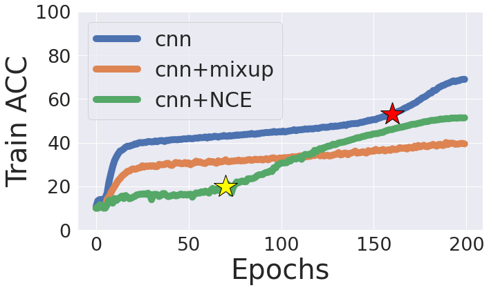
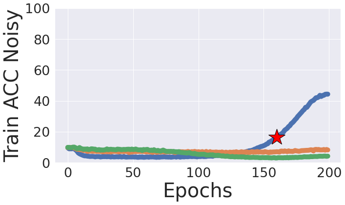
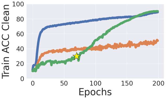
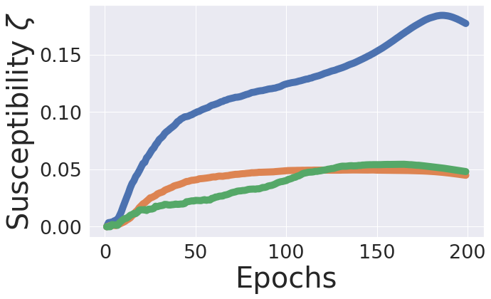
Figure 8: Accuracy on the entire, the clean and the noisy subsets of the training set, versus susceptibility in Equation (2) for a $5-$layer convolutional neural network trained on CIFAR-10 with $50\%$ label noise without any regularization, with Mixup Zhang et al. [2017], and with Active Passive loss using the normalized cross entropy together with reverse cross-entropy loss (denoted by NCE) Ma et al. [2020]. The sharp increases in the overall training accuracy (illustrated by the red and yellow stars) can be caused by an increase in the accuracy of either the clean (the yellow star) or noisy (the red star) subsets. Therefore, this sharp increase could not predict memorization, contrary to the susceptibility $\zeta$, which is strongly correlated with the accuracy on the noisy subset (Pearson correlation between Train ACC Noisy and susceptibility $\zeta$ is $\rho=0.636$).

(a)

(b)

Figure 9: SimBa Guo et al. [2019] adversarial attack success rate versus accuracy on the noisy subset of the training set for networks trained on CIFAR-10 with $50\%$ label noise. To evaluate the robustness of different models with respect to adversarial attacks, we compare the success rate of the adversarial attack SimBa proposed in Guo et al. [2019] after $1000$ iterations. We observe no correlation between the success rate and neither accuracy on the noisy subset nor susceptibility $\zeta$.

Leveraging Unlabeled/Randomly-labeled Data

Unlabeled data has been leveraged previously to predict out-of-distribution performance (when there is a mismatch between the training and test distributions) Garg et al. [2021b]. Li et al. [2019] introduce synthetic noise to unlabeled data, to propose a noise-tolerant meta-learning training approach. Zhang et al. [2021b] use randomly labeled data to perform neural architecture search. In our paper, we leverage unlabeled data to track the memorization of label noise.

Benefits of Memorization

Studies on long-tail data distributions show potential benefits from memorization when rare and atypical instances are abundant in the distribution Feldman [2020], Feldman and Zhang [2020], Brown et al. [2021]. These studies argue that the memorization of these rare instances is required to guarantee low generalization error. On a separate line of work, previous empirical observations suggest that networks trained on noisy labels can still induce good representations from the data, despite their poor generalization performance Li et al. [2020], Maennel et al. [2020]. In this work, we propose an approach to track memorization when noisy labels are present.

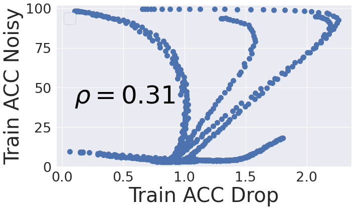
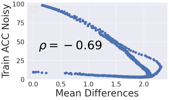
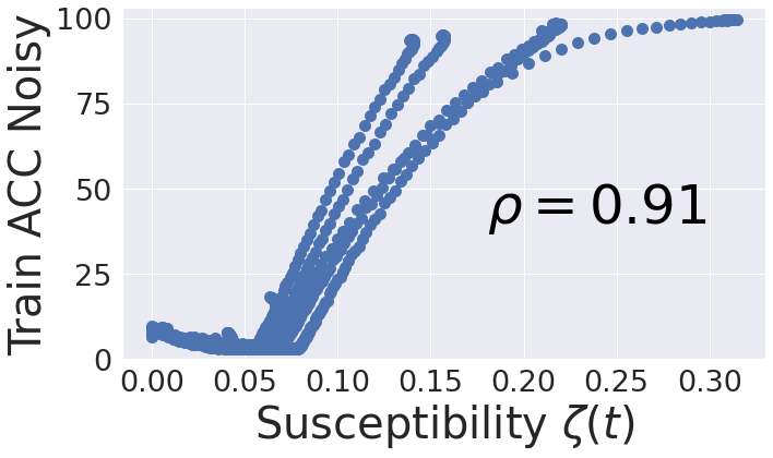
Figure 10: Left: Accuracy on the noisy subset of the training set, versus the training accuracy drop presented in Zhang et al. [2019c] for the following neural network configurations trained on the CIFAR-10 dataset with $50\%$ label noise: a $5$-layer convolutional neural network, DenseNet, EfficientNet, MobileNet, MobileNetV2, RegNet, ResNet, ResNeXt, SENet, and ShuffleNetV2. As proposed in Zhang et al. [2019c], to compute the training accuracy drop, we create a new dataset from the available noisy training set, by replacing $25\%$ of its labels with random labels. We then train these networks on the new dataset, and then compute the difference in the training accuracy of the two setups, divided by $25$ (the level of label noise that was injected). This is reported above as Train ACC Drop. Zhang et al. [2019c] state that desirable networks should have a large drop; therefore there should ideally be a negative correlation between the training accuracy drop and the accuracy on the noisy subset. However, we observe a slightly positive correlation. Therefore, it is difficult to use the results of Zhang et al. [2019c] to track memorization, i.e., training accuracy on the noisy subset. Middle: Accuracy on the noisy subset of the training set, versus the mean difference between the distributions obtained by applying GMM on the training losses, which is proposed in Lu and He [2022] as an early stopping criterion. We observe a negative correlation between the two, and hence conclude that this metric cannot be used to compare memorization of different settings at different stages of training. Right: As opposed to the other two metrics, we observe a strong positive correlation between our metric susceptibility $\zeta$ and memorization.

Theoretical Results

To analyze the convergence of different models on some randomly labeled set, we rely on recent results obtained by modeling the training process of wide neural networks by neural tangent kernels (NTK) Du et al. [2018], Jacot et al. [2018], Allen-Zhu et al. [2018], Arora et al. [2019], Bietti and Mairal [2019], Lee et al. [2019]. In particular, the analysis in our paper is motivated by recent work on convergence analysis of neural networks Du et al. [2018], Arora et al. [2019]. Arora et al. [2019] perform fine-grained convergence analysis for wide two-layered neural networks using gradient descent. They study the convergence of models trained on different datasets (datasets with clean labels versus random labels). In Section 5, we study the convergence of different models trained on some randomly-labeled set. In particular, our models are obtained by training wide two-layered neural networks on datasets with varying label noise levels. As we highlight in the proofs, our work builds on previous art, especially Du et al. [2018], Arora et al. [2019], yet we build in a non-trivial way and for a new problem statement.

Robustness to Adversarial Examples

Deep neural networks are vulnerable to adversarial samples Szegedy et al. [2013], Goodfellow et al. [2014], Akhtar and Mian [2018]: very small changes to the input image can fool even state-of-the-art neural networks. This is an important issue that needs to be addressed for security reasons. To this end, multiple studies towards generating adversarial examples and defending against them have emerged Carlini and Wagner [2017], Papernot et al. [2016b, a], Athalye et al. [2018]. As a side topic related to the central theme of the paper, we examined the connection between models that are resistant to memorization of noisy labels and models that are robust to adversarial attacks. Figure 9 compares the memorization of these models trained on some noisy dataset, with their robustness to adversarial attacks. We do not observe any positive or negative correlation between the two. Some models are robust to adversarial attacks, but perform poorly when trained on datasets with noisy labels, and vice versa. This means that the observations made in this paper are orthogonal to the ongoing discussion regarding the trade-off between robustness to adversarial samples and test accuracy Tsipras et al. [2018], Stutz et al. [2019], Yang et al. [2020], Pedraza et al. [2021], Zhang et al. [2019b], Yin et al. [2019].

Appendix B Experimental Setup

Generating Noisy-labeled Datasets We modify original datasets similarly to Chatterjee [2020]; for a fraction of samples denoted by the label noise level (LNL), we replace the labels with independent random variables drawn uniformly from $\{1,\cdots,c\}$ for a dataset with $c$ number of classes. On average $(1-\text{LNL})+(\text{LNL})\cdot 1/c$ of the samples still have their correct labels. Note that LNL for $\widetilde{S}$ is $1$.

Experiments of Figures 2, 13, 14 and 15 The models at epoch $0$ are pre-trained models on either the clean or noisy versions of the CIFAR-10 dataset for $200$ epochs using SGD with learning rate $0.1$, momentum $0.9$, weight decay $5\cdot 10^{-4}$, and cosineannealing learning rate schedule with $\texttt{T max}=200$. The new sample is a sample drawn from the training set, and its label is randomly assigned to some class different from the correct class label. In Figure 14, the new sample is an unseen sample drawn from the test set.

CIFAR-10 Experiments The models are trained for $200$ epochs on the cross-entropy objective function using SGD with weight decay $5\cdot 10^{-4}$ and batch size $128$. The neural network architecture options are: cnn (a simple $5$-layer convolutional neural network), DenseNet Huang et al. [2017], EfficientNet Tan and Le [2019] (with scale=0.5, 0.75, 1, 1.25, 1.5), GoogLeNet Szegedy et al. [2015], MobileNet Howard et al. [2017] (with scale=0.5, 0.75, 1, 1.25, 1.5), ResNet He et al. [2016a], MobileNetV2 Sandler et al. [2018] (with scale=0.5, 0.75, 1, 1.25, 1.5), Preact ResNet He et al. [2016b], RegNet Radosavovic et al. [2020], ResNeXt Xie et al. [2017], SENet Hu et al. [2018], ShuffleNetV2 Ma et al. [2018] (with scale=0.5, 1, 1.5, 2), DLA Yu et al. [2018], and VGG Simonyan and Zisserman [2014]. The learning rate value options are: $0.001$, $0.005$, $0.01$, $0.05$, $0.1$, $0.5$. The learning rate schedule options are: cosineannealing with T max $200$, cosineannealing with T max $100$, cosineannealing with T max $50$, and no learning rate schedule. Momentum value options are $0.9$, $0$. In addition, we include experiments with Mixup Zhang et al. [2017], active passive losses: normalized cross entropy with reverse cross entropy (NCE+RCE) Ma et al. [2020], active passive losses: normalized focal loss with reverse cross entropy (NFL+RCE) Ma et al. [2020], and robust early learning Xia et al. [2021] regularizers.

CIFAR-100 Experiments The models are trained for $200$ epochs on the cross-entropy objective function using SGD with learning rate $0.1$, weight decay $5\cdot 10^{-4}$, momentum $0.9$, learning rate schedule cosineannealing with T max $200$ and batch size $128$. The neural network architecture options are: cnn, DenseNet, EfficientNet (with scale=0.5, 0.75, 1, 1.25, 1.5), GoogLeNet, MobileNet (with scale=0.5, 0.75, 1, 1.25, 1.5), ResNet, MobileNetV2 (with scale=0.5, 0.75, 1, 1.25, 1.5), RegNet, ResNeXt, ShuffleNetV2 (with scale=0.5, 1, 1.5, 2), DLA, and VGG. In addition, we include experiments with Mixup, active passive losses: NCE+RCE, active passive losses: NFL+RCE, and robust early learning regularizers.

SVHN Netzer et al. [2011] Experiments The models are trained for $200$ epochs on the cross-entropy objective function with learning rate $0.1$ and batch size $128$. The optimizer choices are SGD with weight decay $5\cdot 10^{-4}$, and momentum $0.9$, and Adam optimizers. The learning rate schedule options for the SGD experiments are: cosineannealing with T max $200$, and exponential. The neural network architecture options are: DenseNet, EfficientNet (with scale=0.25, 0.5, 0.75, 1), GoogLeNet (with scale= 0.25, 1, 1.25), MobileNet (with scale= 1, 1.25, 1.5, 1.75), MobileNetV2 (with scale= 1, 1.25, 1.5, 1.75), ResNet (with scale=0.25, 0.5, 1, 1.25, 1.5, 1.75), ResNeXt, SENet (with scale=0.25, 0.5, 0.75, 1), ShuffleNetV2 (with scale=0.25, 0.5, 0.75, 1), DLA (with scale=0.25, 0.5, 0.75, 1), and VGG (with scale=0.25, 0.5, 0.75, 1, 1.25, 1.5, 1.75).

MNIST and Fashion-MNIST Xiao et al. [2017] Experiments The models are trained for $200$ epochs on the cross-entropy objective function with batch size $128$, using SGD with learning rate $0.1$, weight decay $5\cdot 10^{-4}$, and momentum $0.9$. The learning rate schedule options are: cosineannealing with T max $200$, and exponential. The neural network architecture options are: AlexNet Krizhevsky et al. [2012] (with scale=0.25, 0.5, 0.75, 1), ResNet18 (with scale=0.25, 0.5, 0.75, 1), ResNet34 (with scale=0.25, 0.5, 0.75, 1), ResNet50 (with scale=0.25, 0.5, 0.75, 1), VGG11 (with scale=0.25, 0.5, 0.75, 1), VGG13 (with scale=0.25, 0.5, 0.75, 1), VGG16 (with scale=0.25, 0.5, 0.75, 1), VGG19 (with scale=0.25, 0.5, 0.75, 1).

Tiny ImageNet Le and Yang [2015] Experiments The models are trained for $200$ epochs on the cross-entropy objective function with batch size $128$, using SGD with weight decay $5\cdot 10^{-4}$, and momentum $0.9$. The learning rate schedule options are: cosineannealing with T max $200$, exponential, and no learning rate schedule. The learning rate options are: $0.01,0.05,0.1,0.5$. The neural network architecture options are: AlexNet, DenseNet, MobileNetV2, ResNet, SqueezeNet Iandola et al. [2016], and VGG.

Clothing-1M Xiao et al. [2015] Experiments The models are trained for $20$ epochs on the cross-entropy objective function with batch size $128$ using SGD with weight decay $5\cdot 10^{-4}$, and momentum $0.9$. The learning rate schedule options are: cosineannealing with T max $20$, and exponential. The learning rate options are: $0.01,0.005,0.001$. The neural network architecture options are: AlexNet, ResNet18, ResNet 34, ResNeXt, and VGG. Note that because this dataset has random labels we do not introduce synthetic label noise to the labels.

Animal-10N Song et al. [2019] Experiments The models are trained for $50$ epochs on the cross-entropy objective function with batch size $128$ using SGD with weight decay $5\cdot 10^{-4}$, and momentum $0.9$. The learning rate schedule options are: cosineannealing with T max $50$, and exponential. The learning rate options are: $0.001,0.005,0.01$. The neural network architecture options are: ResNet18, ResNet34, SqueezeNet, AlexNet and VGG. Note that because this dataset has random labels we do not introduce synthetic label noise to the labels.

CIFAR-10N Wei et al. [2022] Experiments On these experiments, we work with the aggregate version of the label set which has label noise level of $9\%$ (CIFAR-10N-aggregate in Table 1 of Wei et al. [2022]). The models are trained for 200 epochs on the cross-entropy objective function with batch size $128$ using SGD with weight decay $5\cdot 10^{-4}$, and momentum $0.9$ with cosineannealing learning rate schedule with T max $200$. The learning rate options are: $0.1,0.05$. The neural network architecture options are: cnn, EfficientNet, MobileNet, ResNet, MobileNetV2, RegNet, ResNeXt, ShuffleNetV2, SENet, DLA and VGG.

Each of our experiments take few hours to run on a single Nvidia Titan X Maxwell GPU.

Appendix C Comparison with Baselines

Comparison to a Noisy Validation Set Following the notations from Chen et al. [2021], let the clean and noisy data distributions be denoted by $D$ and $\tilde{D}$, respectively, the classifiers by $h$, and the classification accuracy by $A$. Suppose that the optimal classifier in terms of accuracy on the clean data distribution is $h^{*}$, i.e., $h^{*}=\operatorname*{arg\,max}_{h}A_{D}(h)$. Chen et al. [2021] states that under certain assumptions on the label noise, the accuracy on the noisy data distribution is also maximized by $h^{*}$, that is $h^{*}=\operatorname*{arg\,max}_{h}A_{\tilde{D}}(h)$. However, these results do not allow us to compare any two classifiers $h_{1}$ and $h_{2}$, because we cannot conclude from the results in Chen et al. [2021] that if $A_{D}(h_{1})>A_{D}(h_{2})$, then $A_{\tilde{D}}(h_{1})>A_{\tilde{D}}(h_{2})$. Moreover, it is important to note that these results hold when the accuracy is computed on unlimited dataset sizes. As stated in Lam and Stork [2003], the number of noisy validation samples that are equivalent to a single clean validation sample depends on the label noise level and on the true error rate of the model, which are both unknown in practice. Nevertheless, below we thoroughly compare our approach with having a noisy validation set.

As discussed in Section 4, the susceptibility $\zeta$ together with the training accuracy are able to select models with a high test accuracy. Another approach to select models is to use a subset of the available noisy dataset as a held-out validation set. Table 1 provides the correlation values between the test accuracy on the clean test set and the validation accuracy computed on noisy validation sets with varying sizes. On the one hand, we observe that the correlation between the validation accuracy and the test accuracy is very low for small sizes of the noisy validation set. On the other hand, in the same table, we observe that if the same size is used to compute $\zeta$, our approach provides a high correlation to the test accuracy, even for very small sizes of the held-out set.

In our approach, we first filter out models for which the value of $\zeta$ exceeds a threshold. We set the threshold so that around half of the models remain after this filtration. We then report the correlation between the training and test accuracies among the remaining models. As a sanity check, we doubled checked that, with this filtration, the model with the highest test accuracy was not filtered out.

Size of the set	Train Acc	Val Acc	Our approach
$10$	$0.513$	$0.244$	$\mathbf{0.792}$
$128$		$0.458$	$\mathbf{0.890}$
$256$		$0.707$	$\mathbf{0.878}$
$512$		$0.799$	$\mathbf{0.876}$
$1024$		$0.830$	$\mathbf{0.877}$
$2048$		$0.902$	$\mathbf{0.917}$
$4096$		$0.886$	$\mathbf{0.912}$
$8192$		$\mathbf{0.940}$	${0.923}$
$10000$		$\mathbf{0.956}$	${0.914}$

Table 1: The Kendall $\tau$ correlation between each metric and the test accuracy for CNN, ResNet, EfficientNet, and MobileNet trained on CIFAR-10 with $50\%$ label noise, where the validation accuracy (Val Acc) on a held-out subset of the data and the susceptibility $\zeta$ use a set with the size indicated in each row. We observe that our approach results in a much higher correlation compared to using a noisy validation set. Furthermore, our approach is less sensitive to the size of the held-out set, compared to using a noisy validation set. In particular, to reach the same correlation value, our approach with set size $=10$ is equivalent to using a noisy validation set with size $=512$ (highlighted in red). Also, our approach with set size $=128$ is almost equivalent to using a noisy validation set with size $=1024$ (highlighted in blue). Hence, to use a noisy validation set, one requires around ten-fold the amount of held-out data.

Moreover, in Figure 12, we report the advantage of using our approach compared to using a noisy validation set for various values of the dataset label noise level (LNL) and the size of the set that computes the validation accuracy and susceptibility $\zeta$. We observe that the lower the size of the validation set, and the higher the LNL, the more advantageous our approach is. Note also that for high set sizes and low LNLs, our approach produces comparable results to using a noisy validation set.

Figure 11: The Kendall $\tau$ correlation between our approach and the test accuracy minus the Kendall $\tau$ correlation between validation accuracy (computed on a noisy set) and the test accuracy for various label noise levels (LNL) and set sizes. We observe the advantage of our approach to using a noisy validation set particularly for high LNLs and low set sizes. For other combinations, we also observe comparable results (the correlation difference is very close to zero). Note that the last row can be recovered from the difference in correlation values of Table 1.

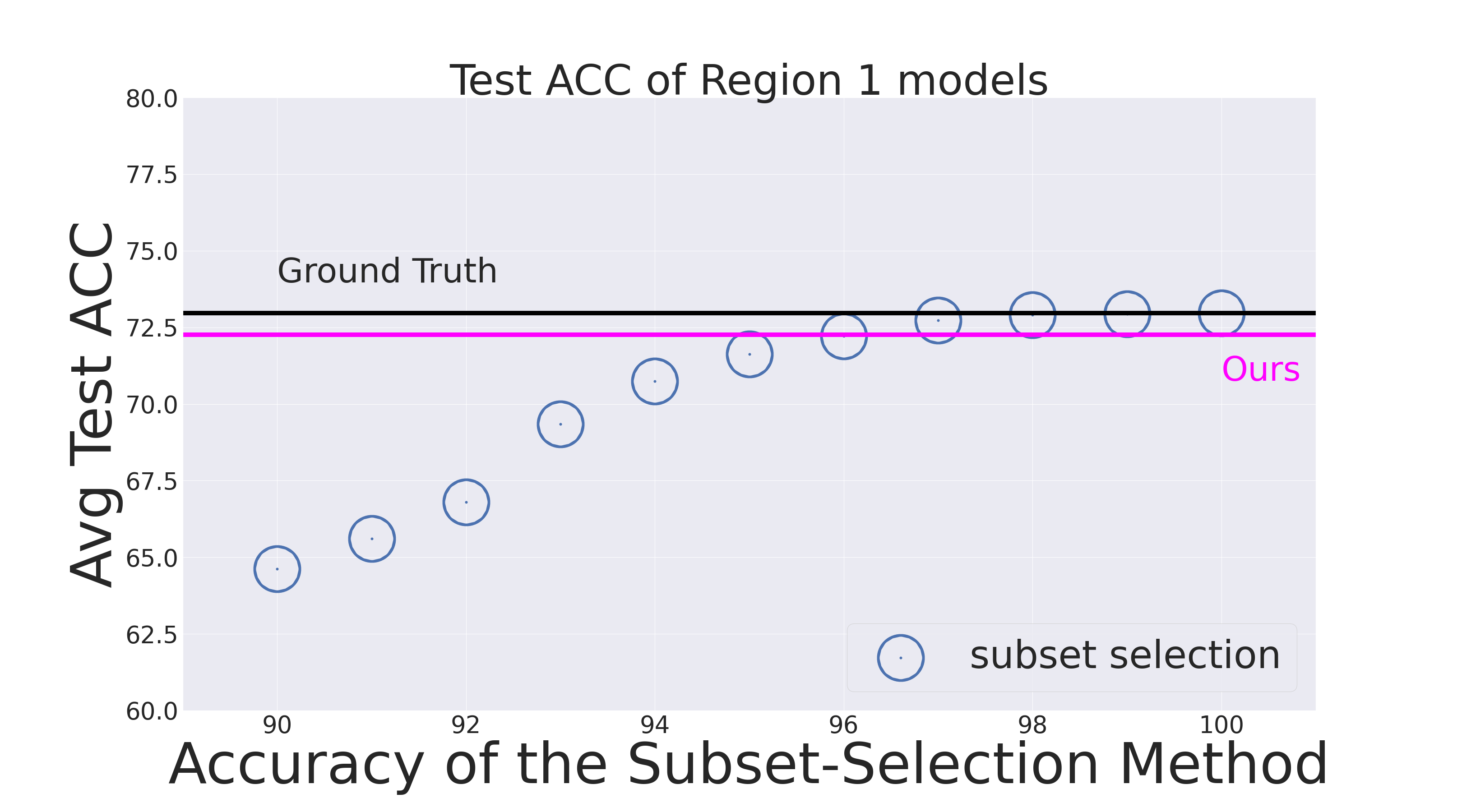
Figure 12: Comparison between the average test accuracy obtained using our approach and the average test accuracy obtained using a method that detects correctly-labeled samples within the training set from the incorrectly-labeled ones with $X\%$ accuracy (the x-axis). The results are obtained from training {CNN, ResNet, EfficientNet, MobileNet}$\times${without regularization, +Mixup, +NCERCE, + NFLRCE, +robust early learning} on CIFAR-10 with $50\%$ label noise. We observe that to have the same performance as our approach, such methods require a very high accuracy (above $96\%$), and even with higher accuracies, our approach gives comparable results.

Comparison to Label Noise Detection Approaches Another line of work is studying methods that detect whether a label assigned to a given sample is correct or not [Zhu et al., 2021, Song et al., 2020b, Pleiss et al., 2020, Pulastya et al., 2021]. Such methods can estimate the clean and noisy subsets. Then, by tracking the training accuracy on the clean and noisy subsets, similar to what is done in Figure 6, they can select models that are located in Region $1$, i.e., that have a low estimated accuracy on the noisy subset and a high estimated accuracy on the clean subset. In Figure 12, we compare the average test accuracy of models selected by our approach with those selected by such subset-selection methods. Let $X$ be the accuracy of the detection of the correct/incorrect label of a sample by the subset selection benchmark: if $X=100\%$, then the method has full access to the ground truth label for each label, if $X=90\%$ the method correctly detects $90\%$ of the labels. We observe a clear advantage of our method for $X$ up to $96\%$, and comparable performance for $X>96\%$.

Appendix D Additional Experiments for Section 2

In this section, we provide additional experiments for the observation presented in Section 2. In Figure 13, we observe that networks with a high test accuracy are resistant to memorizing a new incorrectly-labeled sample. On the other hand, in Figure 14, we observe that networks with a high test accuracy tend to fit a new correctly-labeled sample faster.

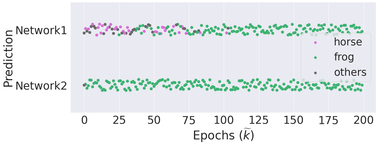
(a)

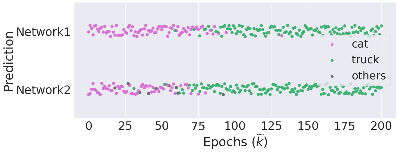
(b)

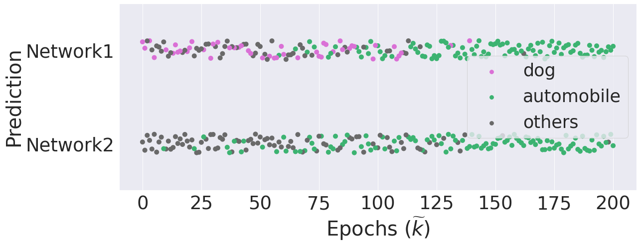
(c)

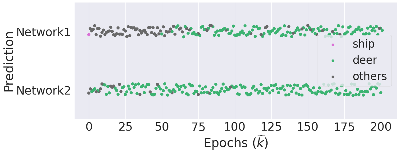
(d)

Figure 13: The evolution of output prediction of two networks that are trained on a single randomly labeled sample. In all sub-figures, Network 1 has a higher test accuracy compared to Network 2, and we observe it is less resistance to memorization of the single incorrectly-labeled sample. Example 1: Network 1 is a ResNeXt trained on CIFAR-10 dataset with $50\%$ random labels and has test accuracy of $58.85\%$. Network 2 is a ResNeXt that is not pre-trained and has test accuracy of $9.74\%$. Example 2: Network 1 is a SENet trained on CIFAR-10 dataset with original labels and has test accuracy of $95.35\%$. Network 2 is a SENet that is trained on CIFAR-10 with $50\%$ label noise and has test accuracy of $56.38\%$. Example 3: Network 1 is a RegNet trained on CIFAR-10 dataset with original labels and has test accuracy of $95.28\%$. Network 2 is a RegNet that is trained on CIFAR-10 with $50\%$ label noise and has test accuracy of $55.36\%$. Example 4: Network 1 is a MobileNet trained on CIFAR-10 dataset with original labels and has test accuracy of $90.56\%$. Network 2 is a MobileNet that is trained on CIFAR-10 with $50\%$ label noise and has test accuracy of $82.76\%$.

(a) Example 1: original label: dog, assigned label: dog

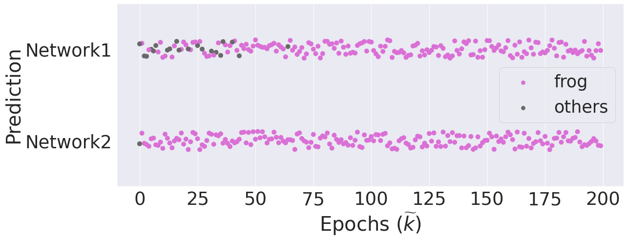
(b)

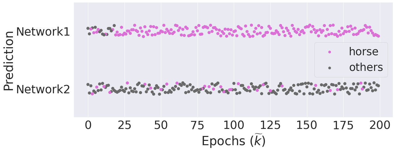
(c)

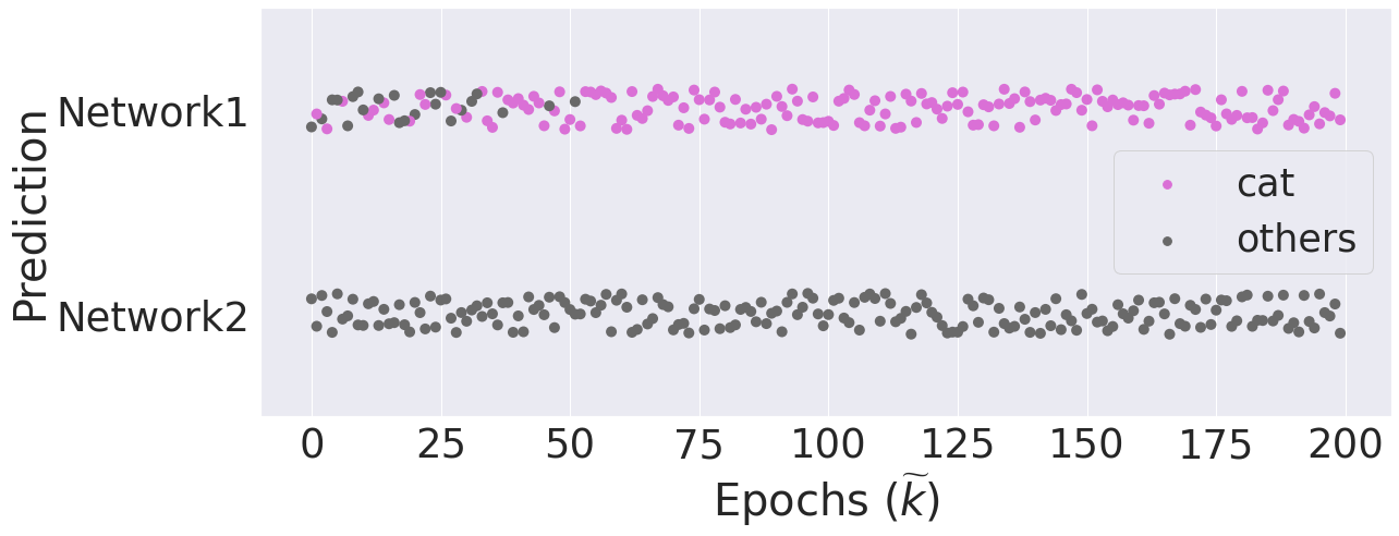
(d)

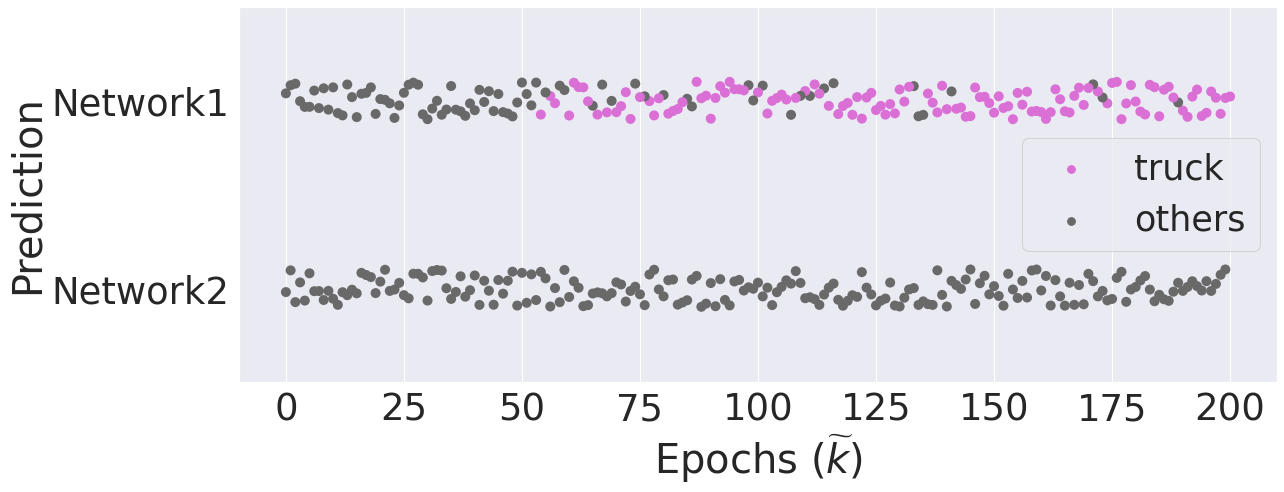
(e)

Figure 14: The evolution of output prediction of two networks that are trained on a single unseen correctly-labeled sample. In all sub-figures, Network 1 has a higher test accuracy compared to Network 2. We observe that give a new correctly-labeled sample Network 2 learns it later, unlike our observation in Figure 2 for a new incorrectly-labeled sample. Example 1: Network 1 is a GoogLeNet trained on CIFAR-10 dataset with clean labels and has test accuracy of $95.36\%$. Network 2 is a GoogLeNet trained on CIFAR-10 dataset with $50\%$ label noise level and has test accuracy of $58.35\%$. Example 2: Network 1 is a ResNeXt trained on CIFAR-10 dataset with $50\%$ random labels and has test accuracy of $58.85\%$. Network 2 is a ResNeXt that is not pre-trained and has test accuracy of $9.74\%$. Example 3: Network 1 is a SENet trained on CIFAR-10 dataset with original labels and has test accuracy of $95.35\%$. Network 2 is a SENet that is trained on CIFAR-10 with $50\%$ label noise and has test accuracy of $56.38\%$. Example 4: Network 1 is a RegNet trained on CIFAR-10 dataset with original labels and has test accuracy of $95.28\%$. Network 2 is a RegNet that is trained on CIFAR-10 with $50\%$ label noise and has test accuracy of $55.36\%$. Example 5: Network 1 is a MobileNet trained on CIFAR-10 dataset with original labels and has test accuracy of $90.56\%$. Network 2 is a MobileNet that is trained on CIFAR-10 with $50\%$ label noise and has test accuracy of $82.76\%$.

Moreover, we study the effect of calibration on the observations of Figures 2 and 13. A poor calibration of a model may affect the confidence in its predictions, which in turn might affect the susceptibility/resistance to new samples. Therefore, in Figure 15, we compare models that have almost the same calibration value. More precisely, Network $1$ is trained on the clean dataset, and Network 2 (calibrated) is a calibrated version of the model that is trained on the noisy dataset using the Temperature scaling approach Guo et al. [2017]. We observe that even with the same calibration level, the model with a higher test accuracy is more resistant to memorizing a new incorrectly-labeled sample.

(a)

(b)

Figure 15: The evolution of output prediction of networks that are trained on a single randomly labeled sample. In all sub-figures, Network 1 (trained on the clean dataset) has a higher test accuracy than Network 2 (trained on the noisy dataset), and we observe it is less resistant to memorization of the single incorrectly-labeled sample. Furthermore, we have ensured using the temperature scaling method Guo et al. [2017] that the two models have the same calibration (ECE) value. Example 1: Network 1 is a GoogleNet trained on CIFAR-10 dataset with original labels and has test accuracy of $95.36\%$. Network 2 is a GoogleNet that is trained on CIFAR-10 with $50\%$ label noise and has test accuracy of $58.35\%$. Example 2: Network 1 is a RegNet trained on CIFAR-10 dataset with original labels and has test accuracy of $95.28\%$. Network 2 is a RegNet that is trained on CIFAR-10 with $50\%$ label noise and has test accuracy of $55.36\%$.

Appendix E Additional Experiments for Section 4

In this section, we provide additional experiments for our main results for MNIST, Fashion-MNIST, SVHN, CIFAR-100, and Tiny Imagenet datasets.

In Figure 16, we observe that for networks trained on the noisy MNIST datasets, models that are resistant to memorization and trainable have on average more than $20\%$ higher test accuracy compared to models that are trainable but not resistant (similar results for other datasets are observed in Figures 18, 20, 23, and 26). Furthermore, without access to the ground-truth, the models with a high (respectively, low) accuracy on the clean (resp., noisy) subsets are recovered using susceptibility $\zeta$ as shown in Figures 21 and 24. Moreover, in Figure 17, we observe that by selecting models with a low value of $\zeta(t)$ the correlation between training accuracy and test accuracy drastically increases from $-0.766$ to $0.863$, which shows the effectiveness of the susceptibility metric $\zeta(t)$ (similar results for other datasets are observed in Figures 19, 22, 25, and 27).

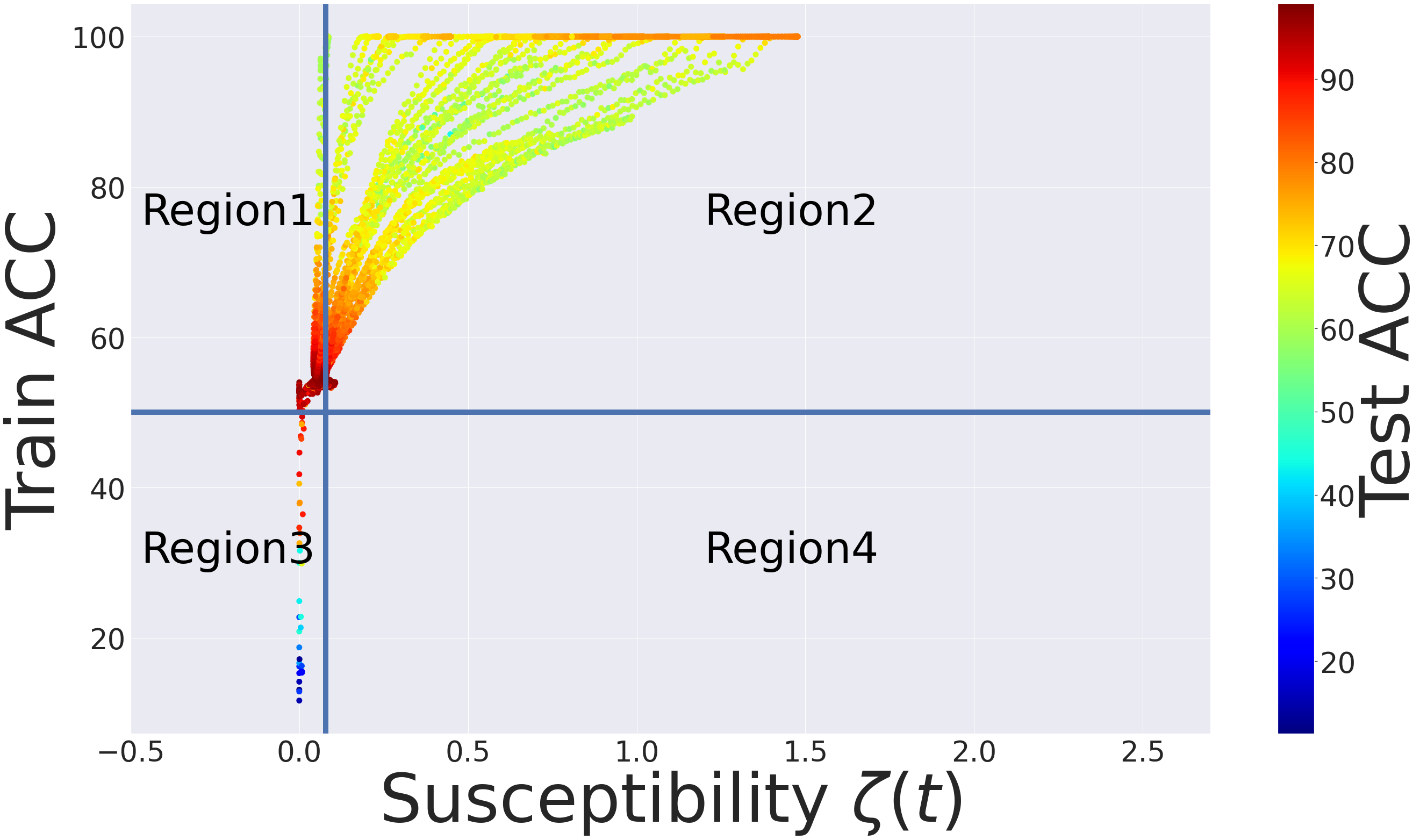
Figure 16: Using susceptibility $\zeta(t)$ and training accuracy, we can obtain 4 different regions for models trained on MNIST with $50\%$ label noise (details in Appendix B). Region 1: Trainable and resistant, with average test accuracy of $95.38\%$. Region 2: Trainable and but not resistant, with average test accuracy of $72.65\%$. Region 3: Not trainable but resistant, with average test accuracy of $47.69\%$. Region 4: Neither trainable nor resistant.

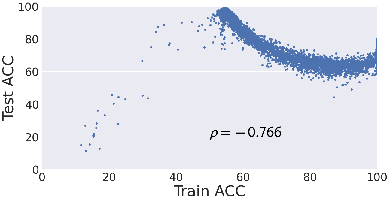
(a)

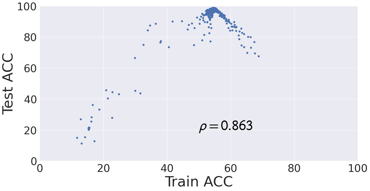
(b)

Figure 17: For models trained on MNIST with $50\%$ label noise (details in Appendix B), the correlation between training accuracy and test accuracy increases a lot by removing models based on the susceptibility metric $\zeta(t)$.

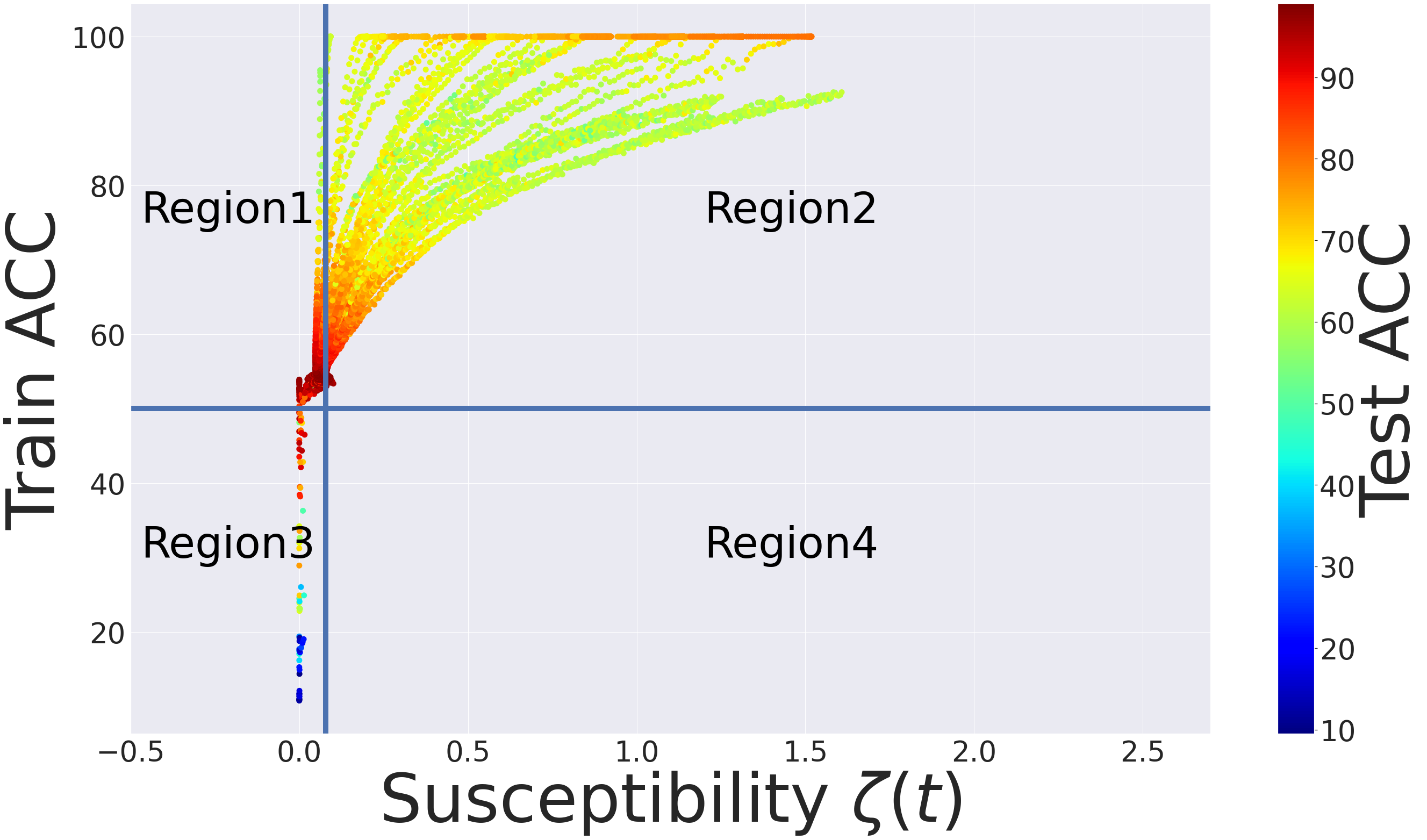
Figure 18: Using susceptibility $\zeta(t)$ and training accuracy we can obtain 4 different regions for models trained on Fashion-MNIST with $50\%$ label noise (details in Appendix B). Region 1: Trainable and resistant, with average test accuracy of $95.82\%$. Region 2: Trainable and but not resistant, with average test accuracy of $72.04\%$. Region 3: not trainable but resistant, with average test accuracy of $52.68\%$. Region 4: Neither trainable nor resistant.

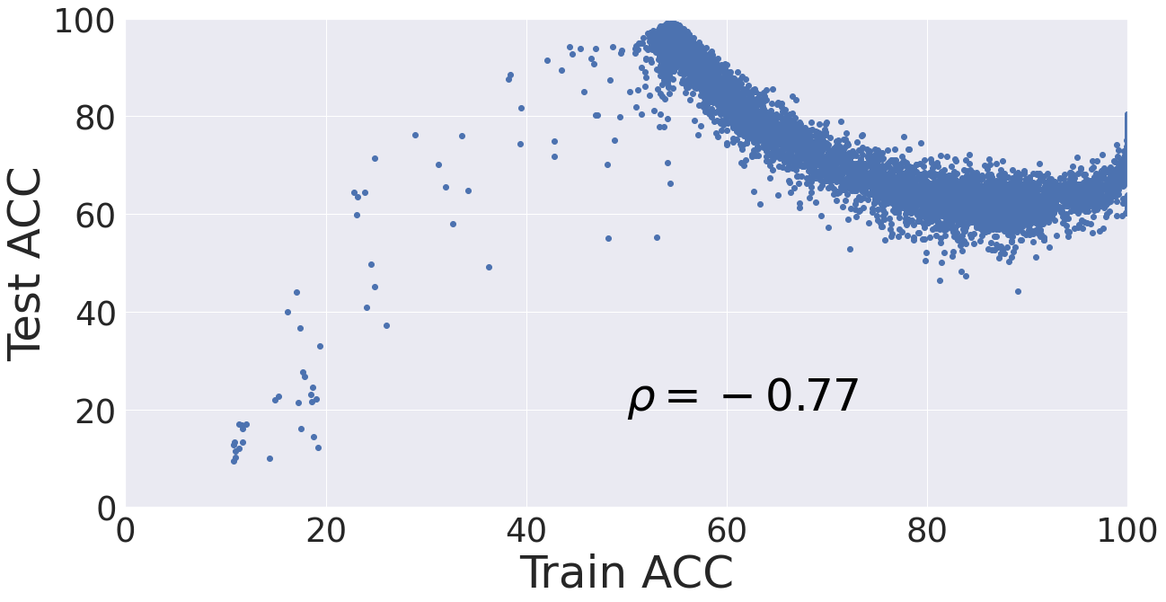
(a)

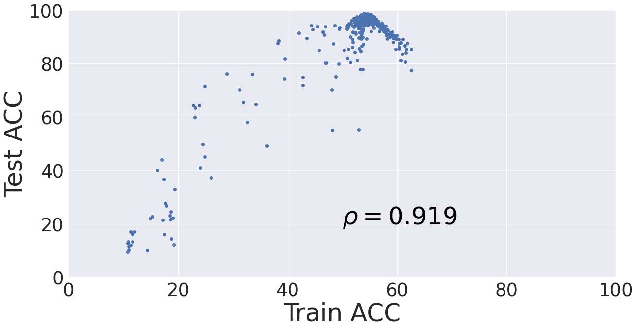
(b)

Figure 19: For models trained on Fashion-MNIST with $50\%$ label noise (details in Appendix B), the correlation between training accuracy and test accuracy increases a lot by removing models based on the susceptibility metric $\zeta(t)$.

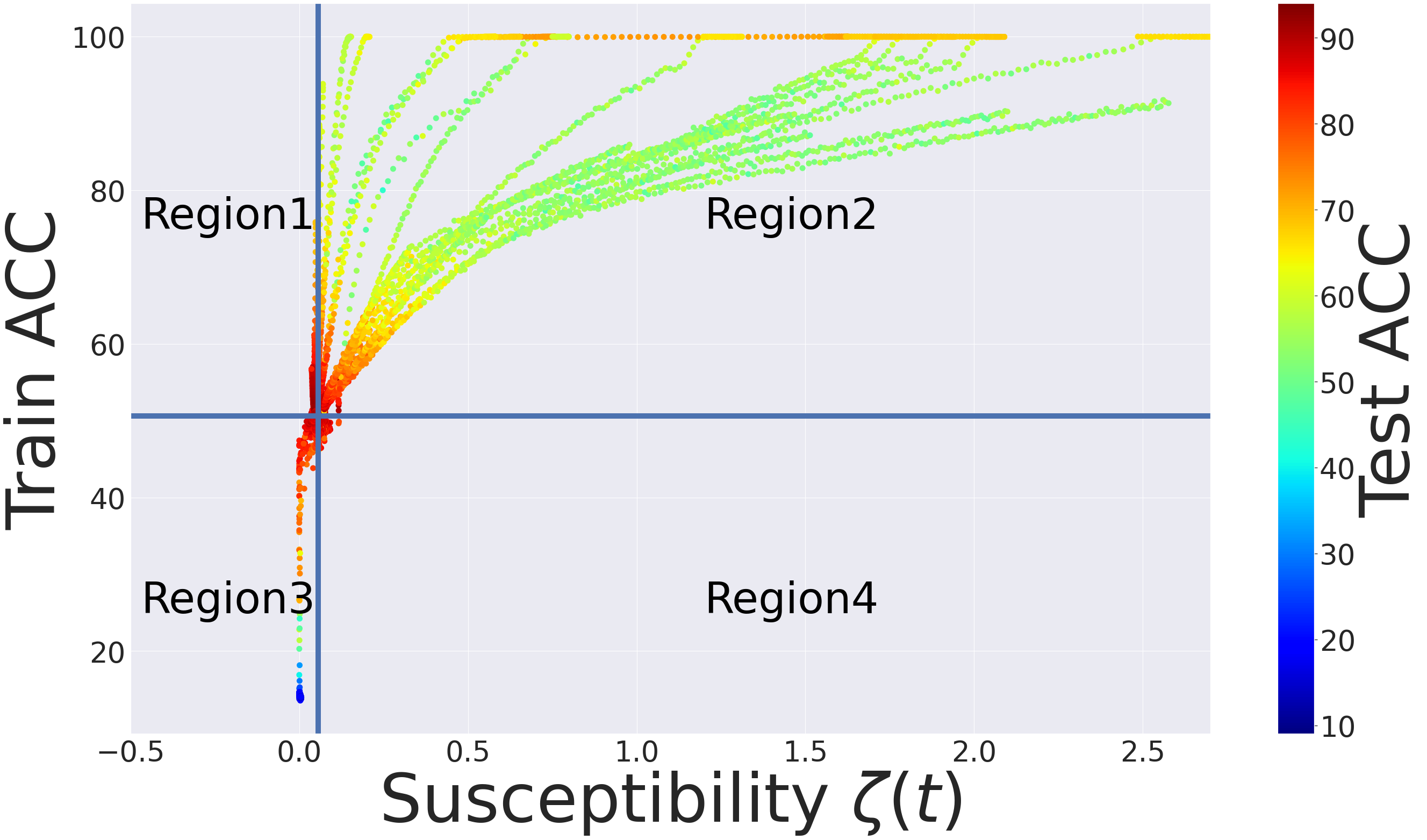
Figure 20: Using susceptibility $\zeta(t)$ and training accuracy we can obtain 4 different regions for models trained on SVHN with $50\%$ label noise (details in Appendix B). Region 1: Trainable and resistant, with average test accuracy of $88.64\%$. Region 2: Trainable and but not resistant, with average test accuracy of $66.34\%$. Region 3: Not trainable but resistant, with average test accuracy of $53.25\%$. Region 4: Neither trainable nor resistant, with average test accuracy of $85.17\%$.

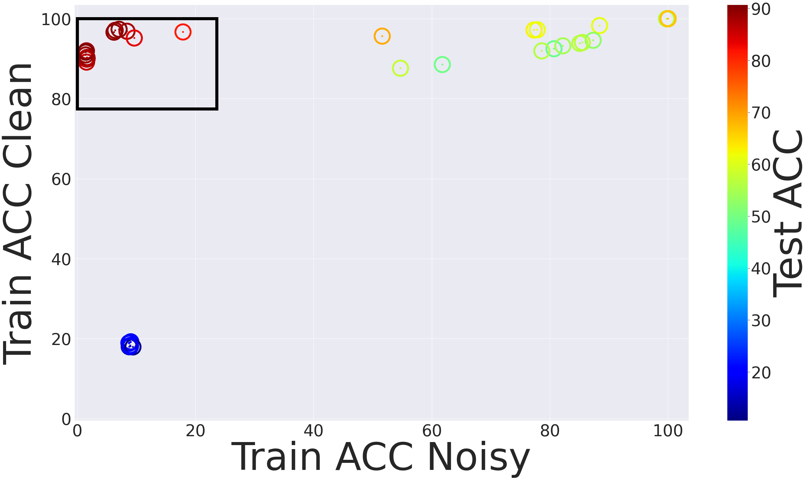
(a) With oracle access to the ground-truth label.
Average test accuracy of the selected models = $87.56\%$

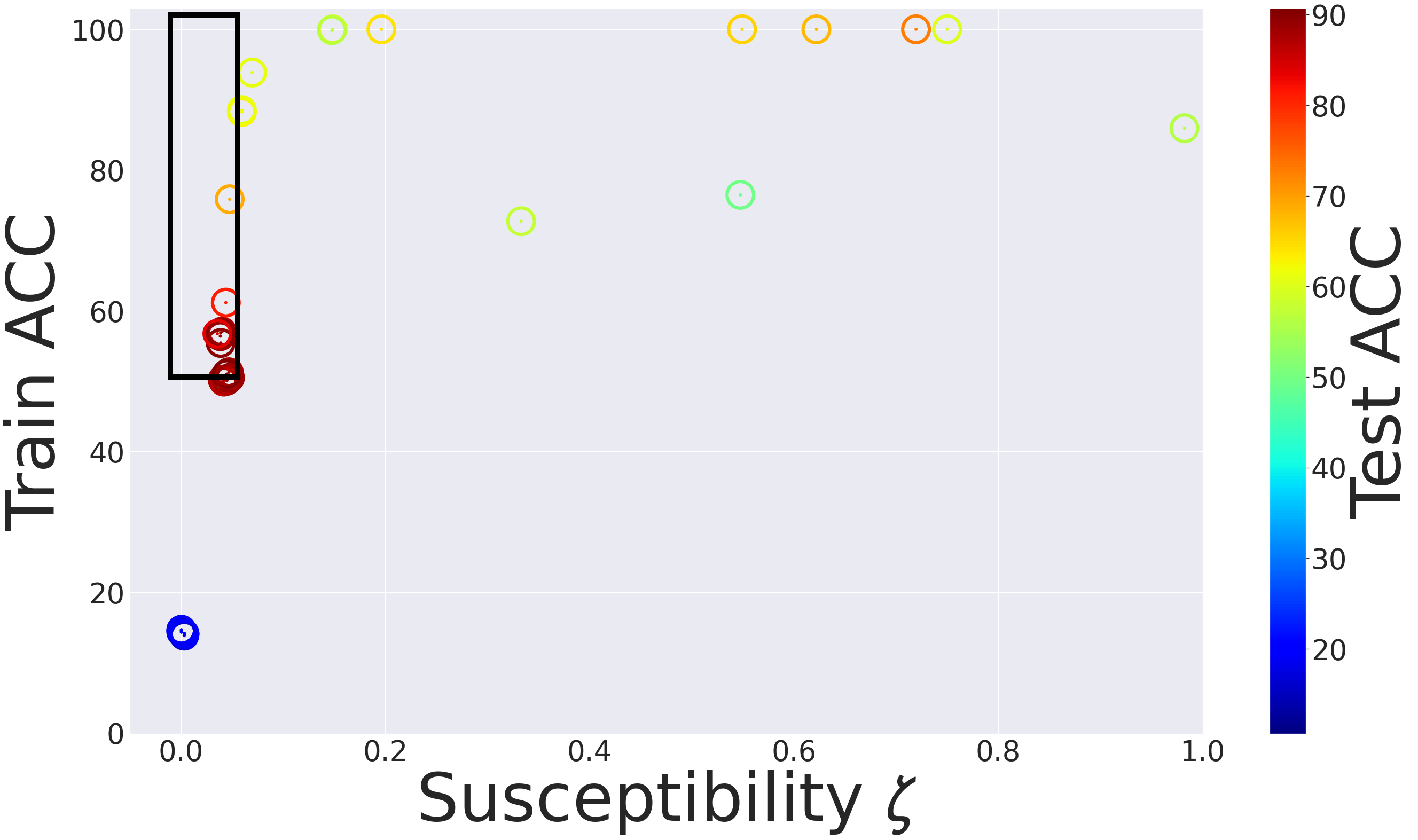
(b) Without access to the ground-truth label.
Average test accuracy of the selected models = $85.44\%$

Figure 21: For models trained on SVHN with $50\%$ label noise (details in Appendix B), with the help of our susceptibility metric $\zeta(t)$ and the overall training accuracy, we can recover models with a high/low accuracy on the clean/noisy subset.

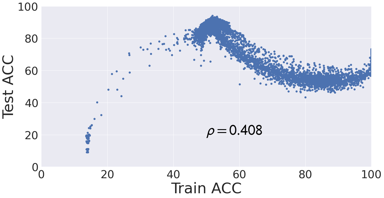
(a)

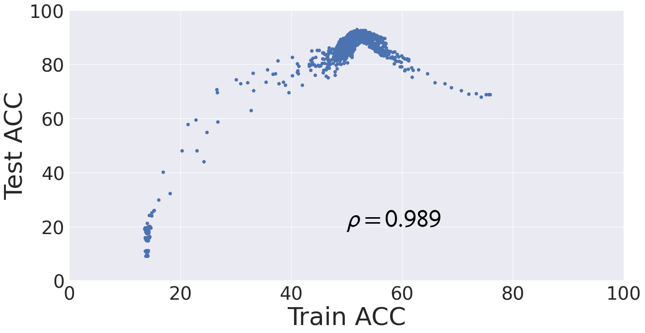
(b)

Figure 22: For models trained on SVHN with $50\%$ label noise (details in Appendix B), the correlation between training accuracy and test accuracy increases a lot by removing models based on the susceptibility metric $\zeta(t)$.

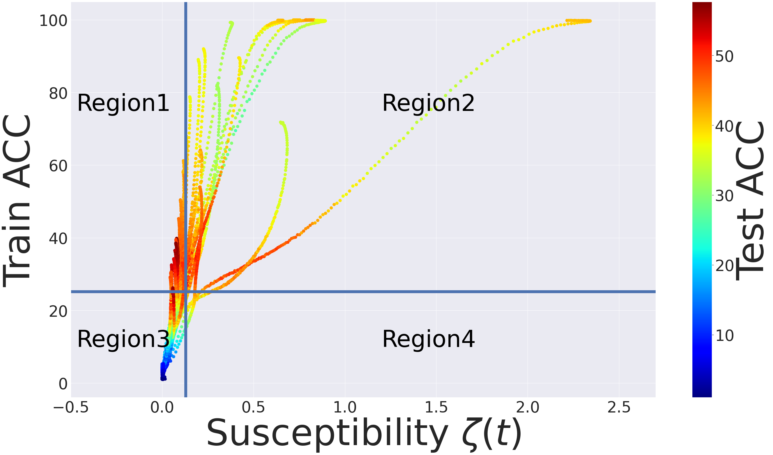
Figure 23: Using susceptibility $\zeta(t)$ and training accuracy we can obtain 4 different regions for models trained on CIFAR-100 with $50\%$ label noise (details in Appendix B). Region 1: Trainable and resistant, with average test accuracy of $47.09\%$. Region 2: Trainable and but not resistant, with average test accuracy of $40.96\%$. Region 3: Not trainable but resistant, with average test accuracy of $22.65\%$. Region 4: Neither trainable nor resistant, with average test accuracy of $39.07\%$.

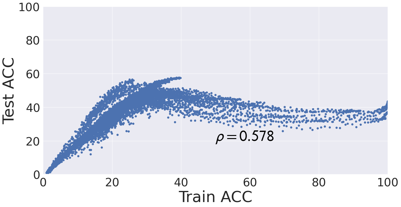
(a)

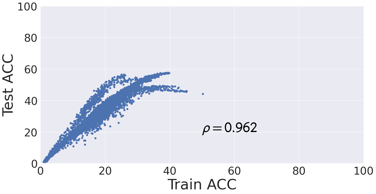
(b)

Figure 25: For models trained on CIFAR-100 with $50\%$ label noise (details in Appendix B), the correlation between training accuracy and test accuracy increases a lot by removing models based on the susceptibility metric $\zeta(t)$.

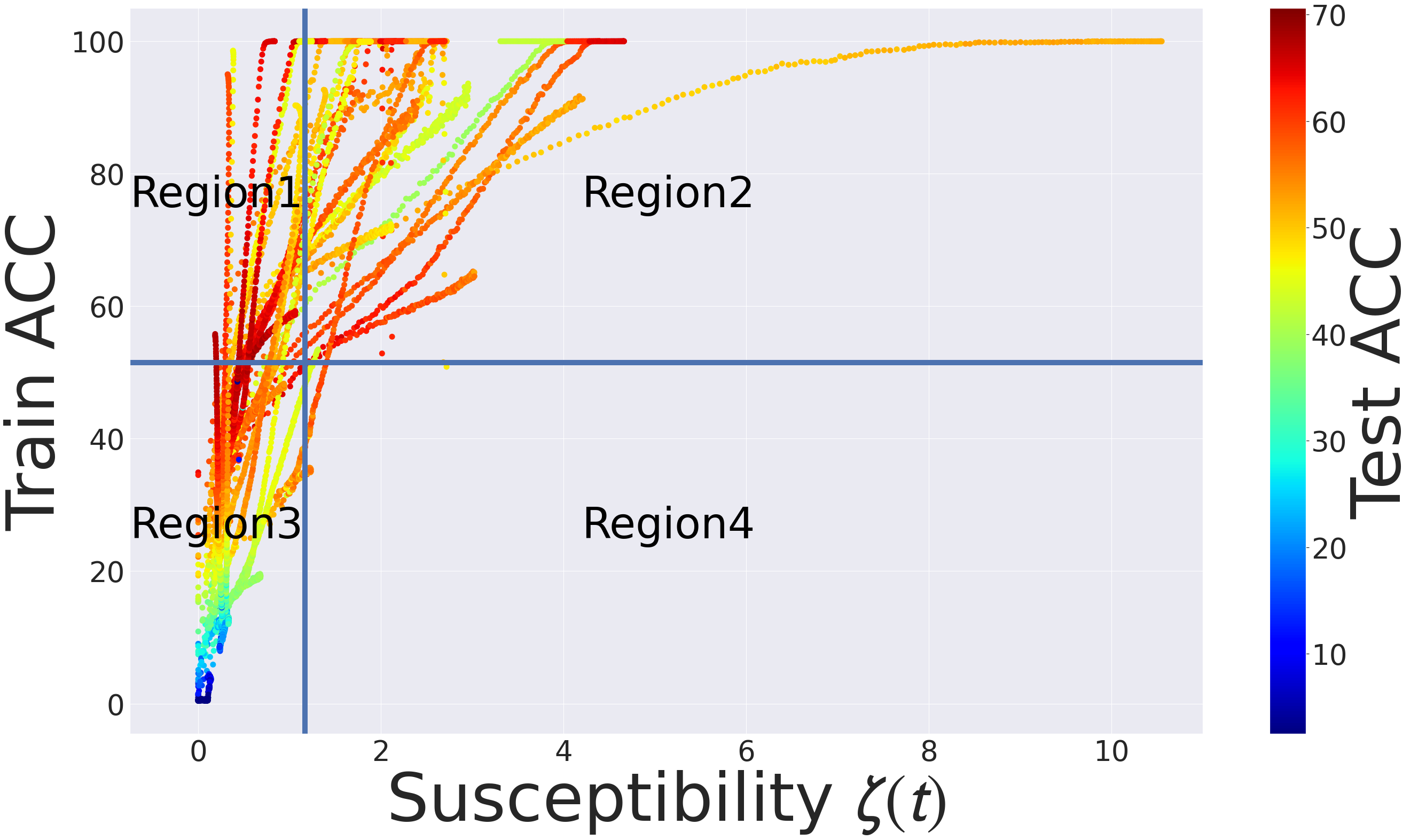
Figure 26: Using susceptibility $\zeta(t)$ and training accuracy we can obtain 4 different regions for models trained on Tiny Imagenet with $10\%$ label noise (details in Appendix B). Region 1: Trainable and resistant, with average test accuracy of $57.51\%$. Region 2: Trainable and but not resistant, with average test accuracy of $53.25\%$. Region 3: Not trainable but resistant, with average test accuracy of $18.53\%$. Region 4: Neither trainable nor resistant, with average test accuracy of $53.26\%$.

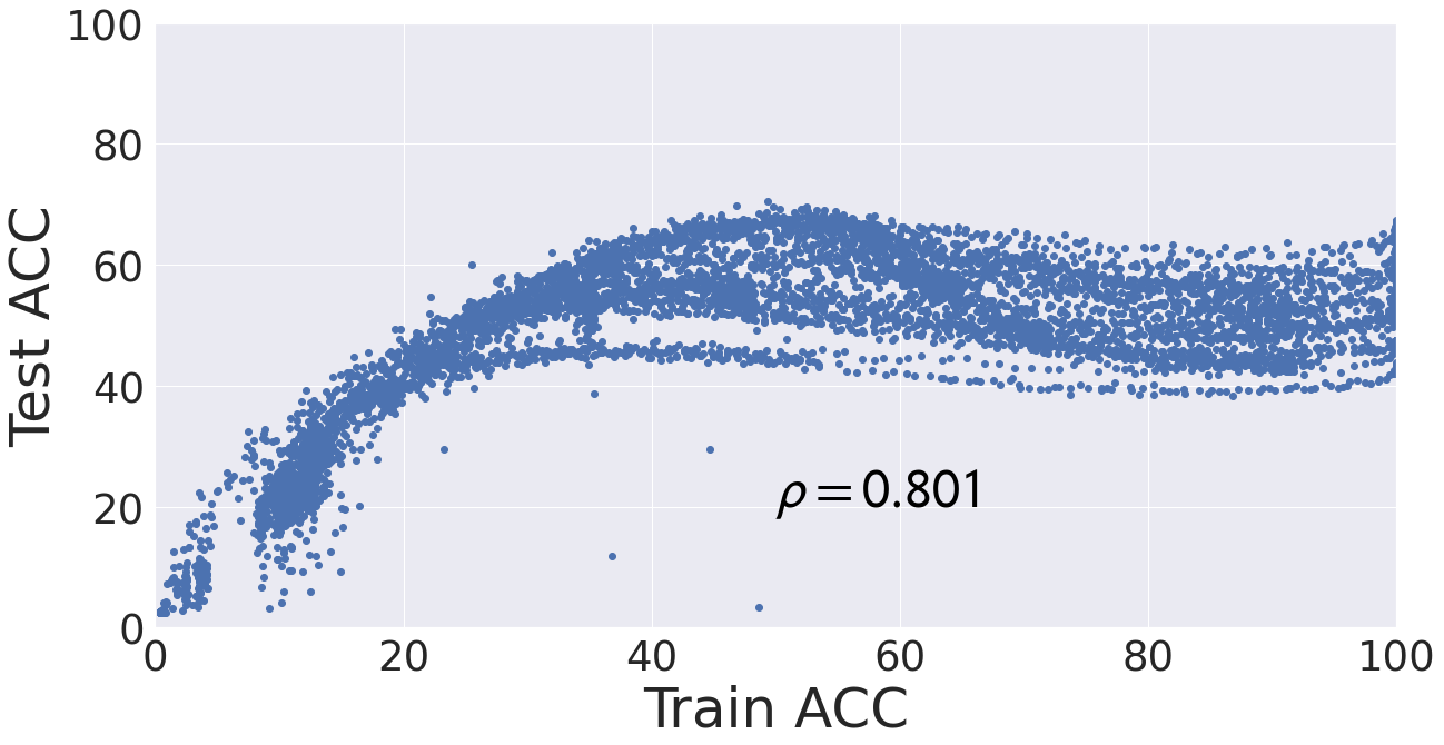
(a)

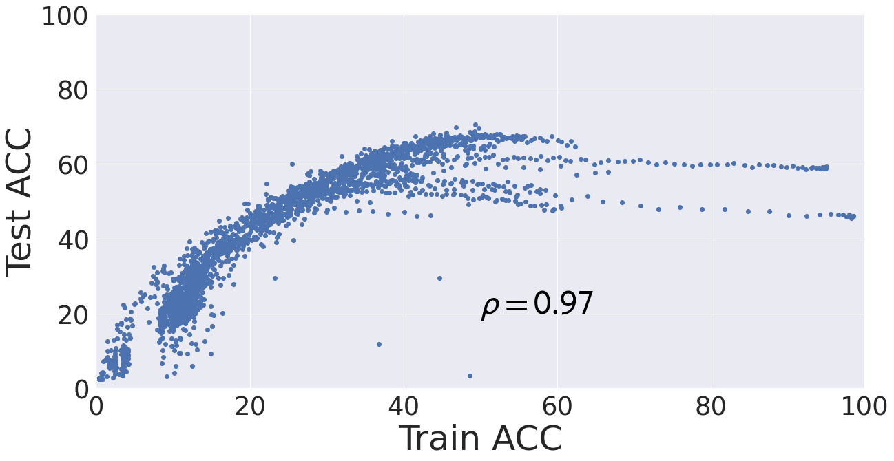
(b)

Figure 27: For models trained on Tiny Imagenet with $10\%$ label noise (details in Appendix B), the correlation between training accuracy and test accuracy increases by removing models based on the susceptibility metric $\zeta(t)$.

Appendix F Experiments Related to Section 7

In this section, we provide some ablation studies that are discussed in Section 7.

In Figure 28, we observe that even among neural network architectures with a good resistance to memorization, susceptibility to noisy labels $\zeta(t)$ detects the most resistant model. We observe that the high correlation between $\zeta$ and memorization of the noisy subset is not limited to a specific learning rate schedule in Figure 29, or a label noise level in Figures 30 and 31. Moreover, in Figures 32 and 33, we observe that for datasets with the label noise level of $10\%$, the susceptibility to noisy labels $\zeta$ and training accuracy still select models with high test accuracy. The same consistency is observed in Figure 36 for models trained with asymmetric label noise.

In the paper, we choose $\widetilde{S}$ to be only a single mini-batch of a randomly-labeled set for computational efficiency. But we also made sure that this does not harm the correlation between Train ACC Noisy and $\zeta(t)$. We analyze the effect of size of $\widetilde{S}$ in Figure 34 (left), which confirms that a single mini-batch is large enough to have a high correlation between Train ACC Noisy and $\zeta(t)$. Moreover, we observe the robustness of the susceptibility metric to the exact choice of the mini-batch in Figure 34 (right).

To better illustrate the match between Train ACC Noisy and $\zeta(t)$, we provide the overlaid curves in Figure 35. This figure clearly shows how using $\zeta$, one can detect/select checkpoints of the model with low memorization.

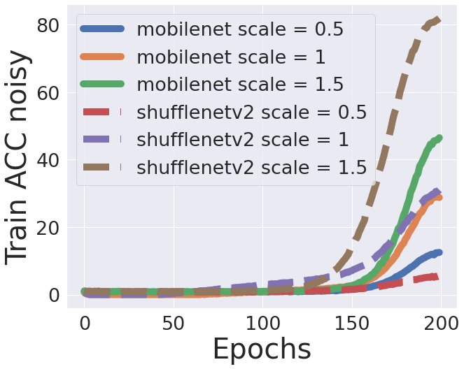
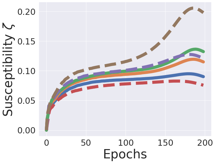
Figure 28: Accuracy on the noisy subset of the training set versus the susceptibility $\zeta(t)$ (Equation (2)) for MobileNet and ShuffleNetV2 configurations trained on CIFAR-100 with $50\%$ label noise. Pearson correlation between the Train ACC Noisy and susceptibility $\zeta$ is $\rho=0.749$. Scale is a hyper-parameter that proportionally scales the number of hidden units and number of channels in the neural network configuration.

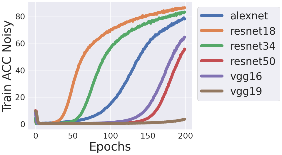
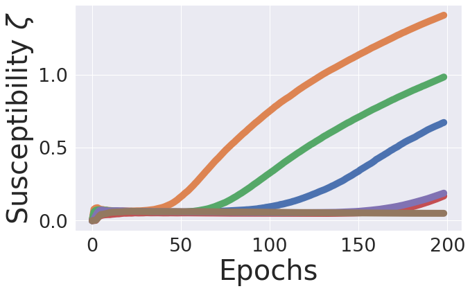
(a)

(b)

Figure 29: Accuracy on the noisy subset of the training set versus the susceptibility $\zeta(t)$ for networks trained on MNIST with $50\%$ label noise. On top and bottom, we have models trained with exponential and cosineannealing learning rate schedulers, respectively. Pearson correlation between Train ACC Noisy and $\zeta$ for exponential and cosineannealing schedules are $\rho=0.89$ and $\rho=0.772$, respectively.

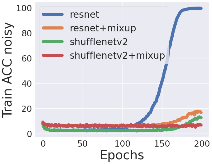
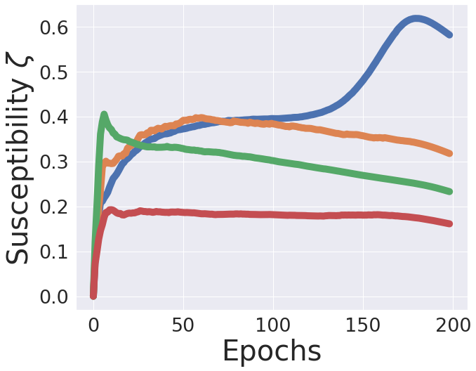
Figure 30: Accuracy on the noisy subset of the training set versus susceptibility to noisy labels $\zeta(t)$ for networks trained on CIFAR-10 with $10\%$ label noise. Pearson correlation between Train ACC Noisy and $\zeta$ is $\rho=0.634$.

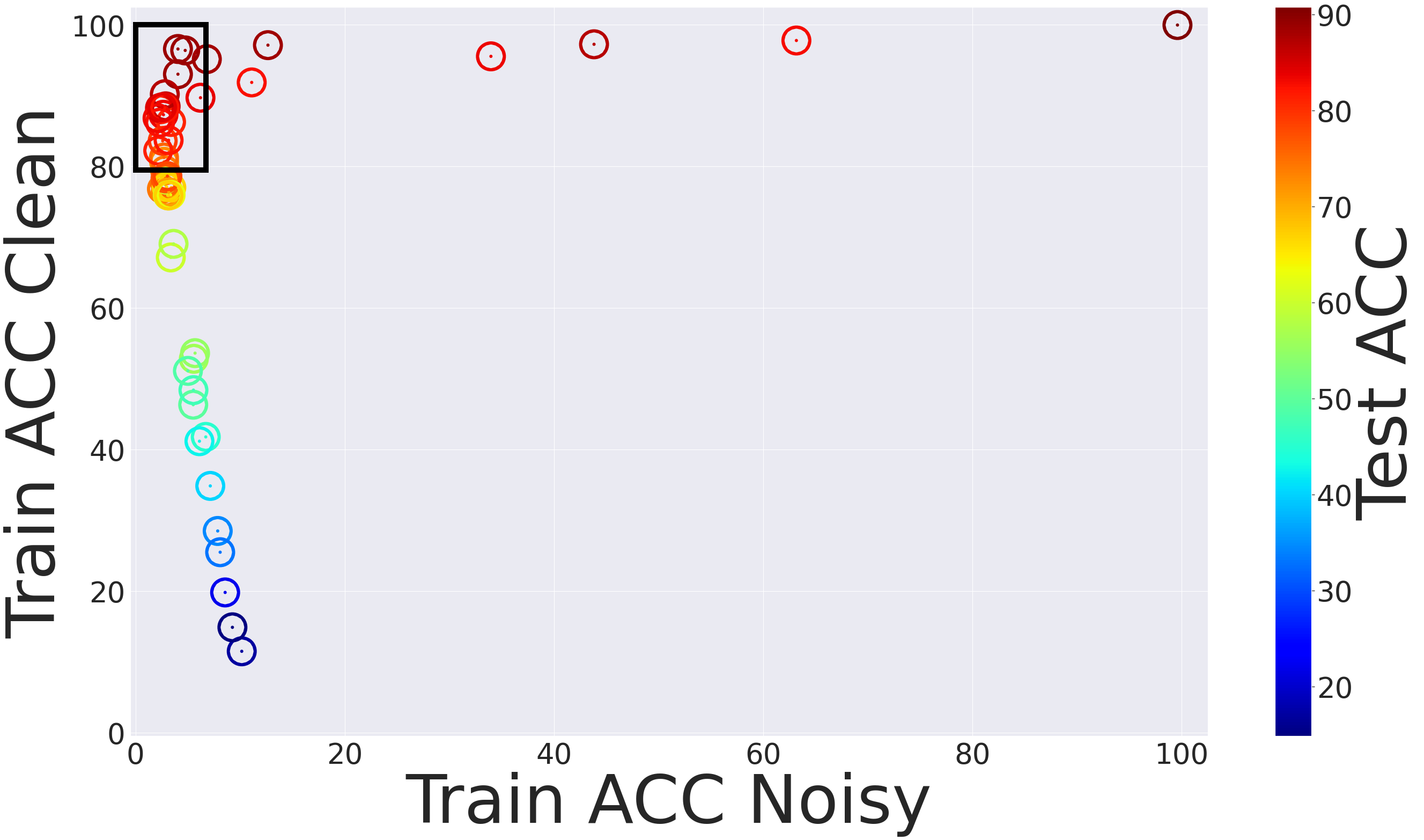
(a) With access to the ground-truth label.
Average test accuracy of the selected models = $82.93\%$

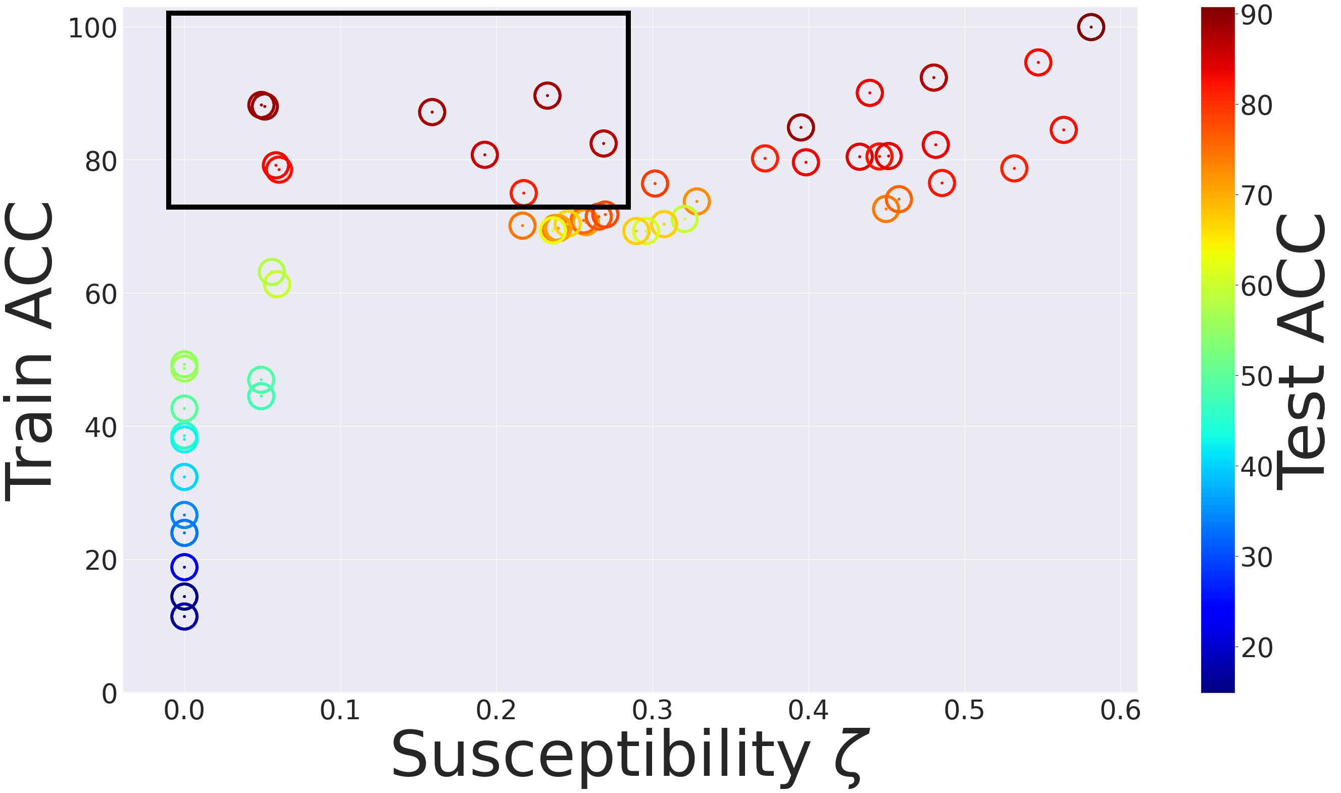
(b) Without access to the ground-truth label. Average test accuracy of the selected models = $86.08\%$

Figure 32: For models trained on CIFAR-10 with $10\%$ label noise for $200$ epochs, using susceptibility $\zeta$ and the overall training accuracy, the average test accuracy of the selected models is comparable with (even higher than) the case of having access to the ground-truth label.

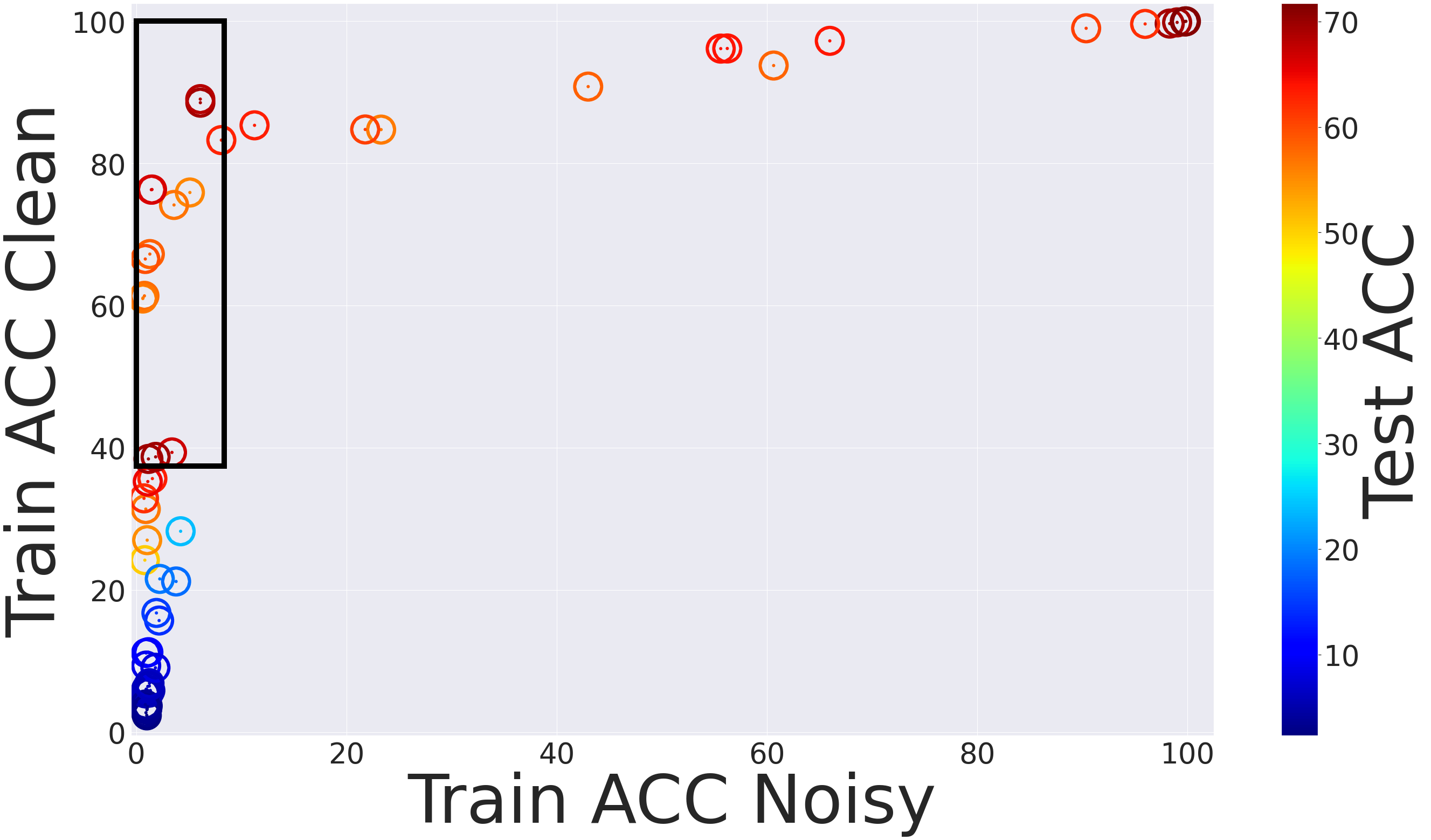
(a) With access to the ground-truth label.
Average test accuracy of the selected models = $62.61\%$

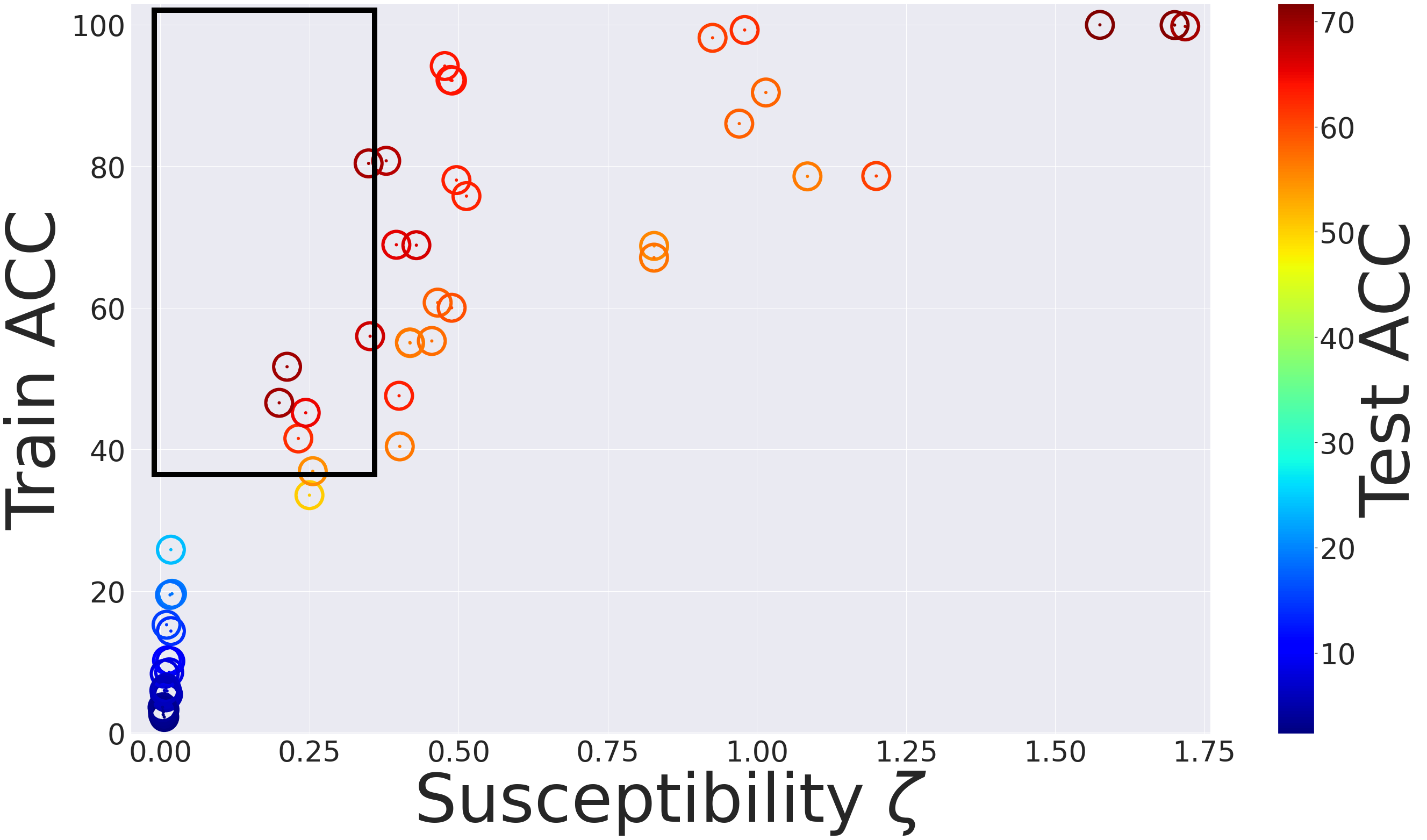
(b) Without access to the ground-truth label. Average test accuracy of the selected models = $64.33\%$

Figure 33: For models trained on CIFAR-100 with $10\%$ label noise for $200$ epochs, using susceptibility $\zeta$ and the overall training accuracy, the average test accuracy of the selected models is comparable with (even higher than) the case of having access to the ground-truth label.

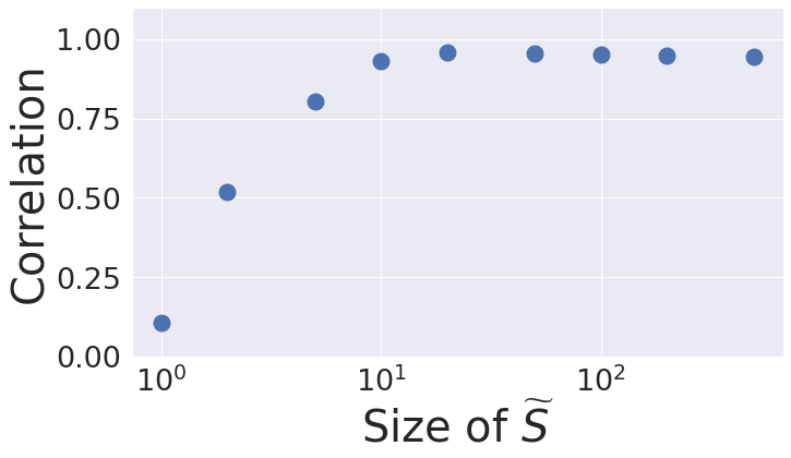
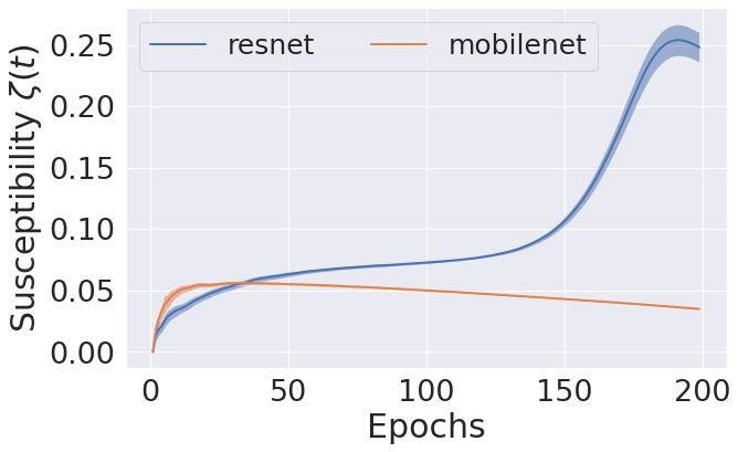
Figure 34: Left: Pearson correlation coefficient between the accuracy on the noisy subset of the training set and susceptibility $\zeta$ (Equation (2)) for different choices of dataset size for $\widetilde{S}$ for ResNet He et al. [2016a], MobileNet Howard et al. [2017], and $5-$layer cnn that are trained on CIFAR-100 dataset with $50\%$ label noise. We observe that unless the dataset is very small, the choice of the dataset size $\widetilde{S}$ does not affect the correlation value. Therefore, throughout our experiments, we choose the size $128$ for this set, which is the batch size used for the regular training procedure as well. Note that this size is very small compared to the size of the training set itself, which is $50000$, hence the computational overhead to compute $\zeta$ is negligible compared to the original training process. Right: We can observe the variance of the susceptibility metric over 10 different random seeds. We can observe that as the variance is quite low, the metric is robust to the exact choice of the mini-batch and to the random labels that are assigned to the mini-batch.

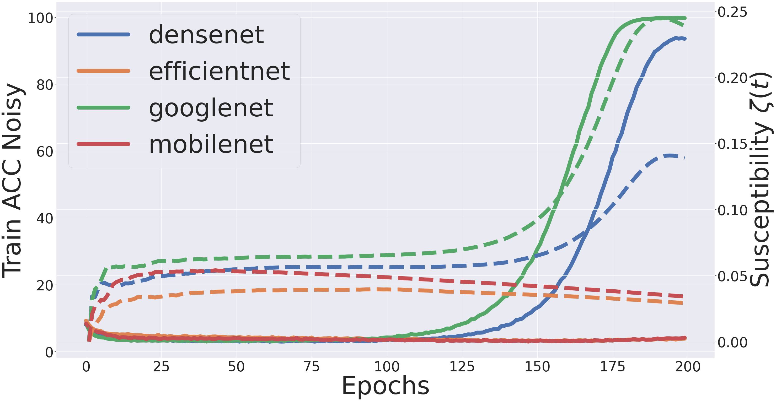
Figure 35: Accuracy on the noisy subset (solid lines) versus Susceptibility $\zeta(t)$ (dashed lines) for neural networks trained on CIFAR-10 with $50\%$ label noise. We observe a very strong match between the two, which suggests that susceptibility can be used to perform early stopping by selecting the checkpoint for each model with the least memorization. For example, for MobileNet and EfficientNet, $\zeta$ does not warn about memorization, hence one can select the end checkpoint. On the other hand, for DenseNet and GoogleNet, $\zeta$ suggests selecting those checkpoints that are before the sharp increases. This is also consistent with the signal given by the fit on the noisy subset, which requires ground-truth label access, unlike susceptibility $\zeta$ which does not require such access.

A study on different thresholds used to select models We would like to point out that if we can tune these thresholds (instead of using the average values of training accuracy and susceptibility over the available models), we can select models with even higher test accuracies than what is reported in our paper. For example, for models of Figure 6, by tuning these two thresholds one could reach a test accuracy of $79.15\%$ (instead of the reported $76\%$) as shown in Figure 37 (left). However, we want to remain in the practical setting where we do not have any access to a clean validation set for tuning. As a consequence, we must avoid any hyper-parameter tuning. And indeed, throughout our experiments, these thresholds are never tuned nor set manually to any extent. Among thresholds that can be computed without access to a clean validation set, we opted for the average values of susceptibility and training accuracy (over the available models) for simplicity. We empirically observe that this choice is robust and produces favorable results in various experimental settings. We could take other percentiles for the threshold, but they are more complex to obtain than simple averages, because they would then depend on the distribution among models. In Figure 37, we study various values of percentiles for these thresholds. We observe that depending on the available models and the given dataset, some other percentiles might give higher test accuracies than simply using the average values. These percentiles range however typically from 35 to 55 and are therefore not far from the mean, hence their benefit in increasing test accuracy appears small compared to the increased complexity to compute them or relying on additional assumptions on the distribution of susceptibility and training accuracy. We observe in Figure 37 (right) that except for very extreme values of the thresholds (which basically select all models as resistant to memorization), the average test accuracy of models in Region 1 is much higher than the average test accuracy of models in Region 2. Hence, our proposed model selection approach is robust to the choice of these thresholds.

Figure 37: Left: Average test accuracy of models in Region 1 of Figure 6 for various thresholds used to find Region 1. In Figure 6 and throughout this paper, Region 1 has models with susceptibility $\zeta$ < t1 and training accuracy > t2, where t1 and t2 are average $\zeta$ and training accuracy over the available models, respectively. Here, we study different values of these thresholds t1 and t2, and their effect on the average test accuracy of models of Region 1. We explore different percentiles of $\zeta$ and training accuracy over all models to be used to find these thresholds. The extreme would be to have $100$th percentiles for both thresholds (low rightmost item of this table), which means models of Region 1 have $\zeta$ < maximum susceptibility and training accuracy > minimum training accuracy. In this extreme case, all models are selected in Region 1. Overall, we observe that some other percentiles might give higher test accuracies than simply using the average values. These percentiles range however typically from 35 to 55 and are therefore not far from the mean, hence their benefit in increasing test accuracy appears small compared to the increased complexity to compute them or relying on additional assumptions on the distribution of susceptibility and training accuracy. Right: The difference in the average test accuracies of models in Region 1 and models in Region 2 for various values of percentiles used to find different regions. A positive value implies that models in Region 1 have a higher average test accuracy. We can observe that except for very extreme values of the thresholds, which basically select all models as trainable, the average test accuracy of models in Region 1 is much higher than the average test accuracy of models in Region 2. Hence, our approach to select resistant and trainable models is robust to the choice of these thresholds.

Appendix G Theoretical Preliminaries

In this section, we provide some technical tools that we use throughout our proofs. Recall from Section 2 that the first layer weights of the neural network are initialized as

$$\mathbf{w}_{r}(0)\sim\mathcal{N}\left(\textbf{0},\kappa^{2}\textbf{I}\right),\quad\forall r\in[m],$$ (7)

where $0<\kappa\leq 1$ is the magnitude of initialization and $\mathcal{N}$ denotes the normal distribution. And the second layer weights $a_{r}$s are independent random variables taking values uniformly in $\{-1,1\}$ at initialization.

G.1 Properties of the Gram-matrix

Properties

Here, we recall a few useful properties of the Gram-matrix (Equation (3)).

1. As shown by Du et al. [2018], $\textbf{H}^{\infty}$ is positive definite and $\lambda_{0}=\lambda_{\text{min}}(\textbf{H}^{\infty})>0$.

2. The matrix $\textbf{H}^{\infty}$ has eigen decomposition $\textbf{H}^{\infty}=\sum_{i=1}^{n}\lambda_{i}\textbf{v}_{i}\textbf{v}_{i}^{T}$, where the eigenvectors are orthonormal. Therefore, $\textbf{v}_{i}^{T}\textbf{v}_{j}=\delta_{i,j}$ for $i,j\in[n]$, the $n\times n$ identity matrix I is decomposed as $\sum_{i=1}^{n}\textbf{v}_{i}\textbf{v}_{i}^{T}$ and any $n$-dimentional (column-wise) vector y can be decomposed as $\textbf{I}\;\textbf{y}=\sum_{i=1}^{n}(\textbf{v}_{i}^{T}\textbf{y})\textbf{v}_{i}$.

3. (Recalled from Du et al. [2018], Arora et al. [2019]) We have $\left\lVert\textbf{H}^{\infty}\right\rVert_{2}\leq\text{tr}(\textbf{H}^{\infty})=\frac{n}{2}=\sum_{i=1}^{n}\lambda_{i}$, and

   $$\eta=O(\frac{\lambda_{0}}{n^{2}})=O\left(\frac{\lambda_{\text{min}}(\textbf{H}^{\infty})}{\left\lVert\textbf{H}^{\infty}\right\rVert_{2}^{2}}\right)\leq\frac{1}{\left\lVert\textbf{H}^{\infty}\right\rVert_{2}}.$$

   Hence,

   $$\left\lVert\textbf{I}-\eta\textbf{H}^{\infty}\right\rVert_{2}\leq 1-\eta\lambda_{0}.$$

G.2 Corollaries Adapted from Du et al. [2018], Arora et al. [2019]

Corollary 1.

(Adapted Theorem 3.1 of Arora et al. [2019] to our setting) For $m=\Omega\left(\frac{n^{6}}{\lambda_{0}^{4}\kappa^{2}\delta^{3}}\right)$ and $\eta=O\left(\frac{\lambda_{0}}{n^{2}}\right)$, for any ${\delta\in(0,1]}$, with probability at least $1-\delta$ over random initialization (7):

$$\Phi\left(\textbf{W}(0)\right)=O\left(\frac{n}{\delta}\right),$$

and

$$\begin{cases}\Phi\left(\textbf{W}(t+1)\right)\leq(1-\frac{\eta\lambda_{0}}{2})\Phi(\textbf{W}(t)),\quad&\text{if}\ 0\leq t<k,\\ \widetilde{\Phi}\left(\textbf{W}(t+1)\right)\leq(1-\frac{\eta\lambda_{0}}{2})\widetilde{\Phi}(\textbf{W}(t)),\quad&\text{if}\ k\leq t<k+\tilde{k}.\end{cases}$$

Therefore, by replacing Equations (1) and (1), throughout the proof we can use:

$$\left\lVert\textbf{f}_{\textbf{W}(0)}-\textbf{y}\right\rVert_{2}=O\left(\sqrt{\frac{n}{\delta}}\right),$$

and

$$\begin{cases}\left\lVert\textbf{f}_{\textbf{W}(t+1)}-\textbf{y}\right\rVert_{2}&\leq\sqrt{1-\frac{\eta\lambda_{0}}{2}}\left\lVert\textbf{f}_{\textbf{W}(t)}-\textbf{y}\right\rVert_{2}\\ &\leq\left(1-\frac{\eta\lambda_{0}}{4}\right)\left\lVert\textbf{f}_{\textbf{W}(t)}-\textbf{y}\right\rVert_{2},\quad\text{if}\ 0\leq t<k,\\ \left\lVert\textbf{f}_{\textbf{W}(t+1)}-\widetilde{\textbf{y}}\right\rVert_{2}&\leq\left(1-\frac{\eta\lambda_{0}}{4}\right)\left\lVert\textbf{f}_{\textbf{W}(t)}-\widetilde{\textbf{y}}\right\rVert_{2},\quad\text{if}\ k\leq t<k+\tilde{k},\end{cases}$$

where we use inequality ${\sqrt{1-\alpha}\leq 1-\alpha/2}$, which holds for $0\leq\alpha\leq 1$.

Corollary 2.

(Adapted from Equation (25) of Arora et al. [2019]) If the parameter vector is updated at step $t$ by one gradient descent step on $\frac{1}{2}\left\lVert\mathbf{f}_{\mathbf{W}(t)}-\mathbf{u}\right\rVert_{2}^{2}$ for some label vector $\mathbf{u}$, and for $t$ such that with probability at least $1-\delta$:

$$\left\lVert\mathbf{H}(t)-\mathbf{H}(0)\right\rVert_{F}=O\left(\frac{n^{3}}{\sqrt{m}\lambda_{0}\kappa\delta^{3/2}}\right),$$

then the output of the neural network is as follows

$$\mathbf{f}_{\mathbf{W}(t+1)}-\mathbf{f}_{\mathbf{W}(t)}=-\eta\mathbf{H}^{\infty}\left(\mathbf{f}_{\mathbf{W}(t)}-\mathbf{u}\right)+\xi(t),$$

where $\xi(\cdot)$ is considered to be a perturbation term that can be bounded with probability at least $1-\delta$ over random initialization (7) by

$$\left\lVert\xi(t)\right\rVert_{2}=O\left(\frac{\eta n^{3}}{\sqrt{m}\lambda_{0}\kappa\delta^{3/2}}\right)\left\lVert\mathbf{f}_{\mathbf{W}(t)}-\mathbf{u}\right\rVert_{2}.$$ (8)

Remark: In our setting, this corollary holds for $0\leq t\leq k-1$ with $\textbf{u}=\textbf{y}$, and for $k\leq t\leq k+\tilde{k}-1$ with $\textbf{u}=\widetilde{\textbf{y}}$. We only need to show that for our setting for $t\geq k$, $\left\lVert\mathbf{H}(t)-\mathbf{H}(0)\right\rVert_{F}$ is bounded, which is done in Lemma 3.

Corollary 3.

(From Equation (27) of Arora et al. [2019]) We have for $1\leq t\leq k$

$$\mathbf{f}_{\mathbf{W}(t)}-\mathbf{{y}}=\left(\mathbf{I}-\eta\mathbf{H}^{\infty}\right)^{t}\left(\mathbf{f}_{\mathbf{W}(0)}-\mathbf{{y}}\right)+\sum_{s=0}^{t-1}\left(\mathbf{I}-\eta\mathbf{H}^{\infty}\right)^{s}\xi\left(t-s-1\right),$$

where $\left\lVert\xi(\cdot)\right\rVert_{2}$ is some perturbation term that can be bounded using Equation (8) with $\mathbf{u}=\mathbf{y}$.

G.3 Additional Lemmas

Lemma 1.

For the setting described in Section 2, we have

$$\mathbf{f}_{\mathbf{W}(k)}-\widetilde{\mathbf{y}}=\sum_{i=1}^{n}\left[(\mathbf{v}_{i}^{T}\mathbf{y})-\left(1-\eta\lambda_{i}\right)^{k}(\mathbf{v}_{i}^{T}\mathbf{y})-(\mathbf{v}_{i}^{T}\widetilde{\mathbf{y}})\right]\mathbf{v}_{i}+\chi(k),$$ (9)

where $\chi(k)$ is some perturbation term that with probability at least $1-\delta$ over the random initialization (7)

$$\left\lVert\chi(k)\right\rVert_{2}=O\left(\frac{n^{3/2}\kappa}{\sqrt{\delta}\lambda_{0}}+\frac{n^{9/2}}{\sqrt{m}\lambda_{0}^{3}\kappa\delta^{2}}\right).$$ (10)

G.3.1 Lemmas to Bound $\textbf{H}(t)$ with $\textbf{H}^{\infty}$

Because the two datasets $S$ and $\widetilde{S}$ have the same input samples, the Gram matrix defined in Equation (3) is the same for both of them. We now recall two lemmas from Du et al. [2018], Arora et al. [2019] and provide a lemma extending them to bound $\textbf{H}(t)$ with $\textbf{H}^{\infty}$, where

$$\textbf{H}_{ij}(t)=\frac{\textbf{x}_{i}^{T}\textbf{x}_{j}}{m}\sum_{r=1}^{m}\mathbb{I}_{r,i}(t)\mathbb{I}_{r,j}(t),$$

and $\mathbb{I}_{r,i}(t)=\mathbb{I}\{\textbf{w}_{r}^{T}(t)\textbf{x}_{i}\geq 0\}$.

Lemma 2.

(recalled from Du et al. [2018], Arora et al. [2019]) For $\lambda_{0}=\lambda_{\text{min}}(\textbf{H}^{\infty})>0$, $m=\Omega\left(\frac{n^{6}}{\lambda_{0}^{4}\kappa^{2}\delta^{3}}\right)$, and $\eta=O\left(\frac{\lambda_{0}}{n^{2}}\right)$ with probability at least $1-\delta$ over the random initialization (7), for all $0\leq t\leq k$, we have:

$$\left\lVert\textbf{H}(t)-\textbf{H}(0)\right\rVert_{F}=O\left(\frac{n^{3}}{\sqrt{m}\lambda_{0}\kappa\delta^{3/2}}\right).$$

Lemma 3.

(Our extension) For $\lambda_{0}=\lambda_{\text{min}}(\textbf{H}^{\infty})>0$, $m=\Omega\left(\frac{n^{6}}{\lambda_{0}^{4}\kappa^{2}\delta^{3}}\right)$, and $\eta=O\left(\frac{\lambda_{0}}{n^{2}}\right)$ with probability at least $1-\delta$ over the random initialization (7), for all $k+1\leq t\leq k+\tilde{k}$, we have:

$$\left\lVert\textbf{H}(t)-\textbf{H}(0)\right\rVert_{F}=O\left(\frac{n^{3}}{\sqrt{m}\lambda_{0}\kappa\delta^{3/2}}\right).$$

Lemma 4.

(recalled from Du et al. [2018], Arora et al. [2019]) With probability at least $1-\delta$ over the random initialization (7), we have:

$$\left\lVert\textbf{H}(0)-\textbf{H}^{\infty}\right\rVert_{F}=O\left(\frac{n\sqrt{\log\frac{n}{\delta}}}{\sqrt{m}}\right).$$

Remark for Lemma 4: The indicator function $\mathbb{I}\{\textbf{w}_{r}(t)^{T}\textbf{x}_{i}\geq 0\}$ is invariant to the scale $\kappa$ of $\textbf{w}_{r}$, hence $\mathbb{E}[\textbf{H}_{ij}(0)]=\textbf{H}_{ij}^{\infty}$, even though the expectation on the left hand side is taken with respect to $\textbf{w}\sim\mathcal{N}(\textbf{0},\kappa^{2}\textbf{I})$ and the expectation on the right hand side is taken with respect to $\textbf{w}\sim\mathcal{N}(\textbf{0},\textbf{I})$.

Appendix H Proof of Lemma 3

Proof.

We recall from the proof of Lemma C.2 of Arora et al. [2019] that if with probability at least $1-\delta$, $\left\lVert\textbf{w}_{r}(t)-\textbf{w}_{r}(0)\right\rVert_{2}\leq R$, then with probability at least $1-\delta$, we have $\left\lVert\textbf{H}(t)-\textbf{H}(0)\right\rVert_{F}\leq\frac{4n^{2}R}{\sqrt{2\pi}\kappa\delta}+\frac{2n^{2}}{m}$. So, we first find an upper bound on $\left\lVert\textbf{w}_{r}(t)-\textbf{w}_{r}(0)\right\rVert_{2}$ for $t>k$ and replace its value $R$ in $\frac{4n^{2}R}{\sqrt{2\pi}\kappa\delta}+\frac{2n^{2}}{m}$.

To find an upper bound on $\left\lVert\textbf{w}_{r}(t)-\textbf{w}_{r}(0)\right\rVert_{2}$ for $t>k$, we can follow a similar approach as in the proof of Lemma C.1 of Arora et al. [2019]:

$$\left\lVert\textbf{w}_{r}(t)-\textbf{w}_{r}(0)\right\rVert_{2}\leq\sum_{\tau=0}^{t-1}\left\lVert\textbf{w}_{r}(\tau+1)-\textbf{w}_{r}(\tau)\right\rVert_{2}$$ (11)

$$=\sum_{\tau=0}^{k-1}\left\lVert\textbf{w}_{r}(\tau+1)-\textbf{w}_{r}(\tau)\right\rVert_{2}+\sum_{\tau=k}^{t-1}\left\lVert\textbf{w}_{r}(\tau+1)-\textbf{w}_{r}(\tau)\right\rVert_{2}$$

$$\overset{(a)}{\leq}\sum_{\tau=0}^{k-1}\frac{\eta\sqrt{n}}{\sqrt{m}}\left\lVert\textbf{f}_{\textbf{W}(\tau)}-\textbf{y}\right\rVert_{2}+\sum_{\tau=k}^{t-1}\frac{\eta\sqrt{n}}{\sqrt{m}}\left\lVert\textbf{f}_{\textbf{W}(\tau)}-\widetilde{\textbf{y}}\right\rVert_{2}$$

$$\overset{(b)}{\leq}\sum_{\tau=0}^{k-1}\frac{\eta\sqrt{n}}{\sqrt{m}}\left(1-\frac{\eta\lambda_{0}}{4}\right)^{\tau}\left\lVert\textbf{f}_{\textbf{W}(0)}-\textbf{y}\right\rVert_{2}$$

$$+\sum_{\tau=k}^{t-1}\frac{\eta\sqrt{n}}{\sqrt{m}}\left(1-\frac{\eta\lambda_{0}}{4}\right)^{\tau-k}\left\lVert\textbf{f}_{\textbf{W}(k)}-\widetilde{\textbf{y}}\right\rVert_{2}$$

$$\overset{(c)}{\leq}O\left(\frac{\eta n}{\sqrt{m\delta}}\right)\sum_{\tau=0}^{k-1}\left(1-\frac{\eta\lambda_{0}}{4}\right)^{\tau}$$

$$+\sum_{\tau=k}^{t}\frac{\eta\sqrt{n}}{\sqrt{m}}\left(1-\frac{\eta\lambda_{0}}{4}\right)^{\tau-k}\left[\left\lVert\textbf{f}_{\textbf{W}(k)}-{\textbf{y}}\right\rVert_{2}+\left\lVert\widetilde{\textbf{y}}-{\textbf{y}}\right\rVert_{2}\right]$$

$$\overset{(d)}{\leq}O\left(\frac{\eta n}{\sqrt{m\delta}}\right)\sum_{\tau=0}^{k-1}\left(1-\frac{\eta\lambda_{0}}{4}\right)^{\tau}+O\left(\frac{\eta n}{\sqrt{m\delta}}\right)\sum_{\tau=0}^{t-k}\left(1-\frac{\eta\lambda_{0}}{4}\right)^{\tau}$$

$$\leq O\left(\frac{\eta n}{\sqrt{m\delta}}\right)\sum_{\tau=0}^{\infty}\left(1-\frac{\eta\lambda_{0}}{4}\right)^{\tau}\leq O\left(\frac{n}{\lambda_{0}\sqrt{m\delta}}\right),$$

where $(a)$ holds because for an update step on label vector u according to gradient descent, we have

$$\left\lVert\textbf{w}_{r}(\tau+1)-\textbf{w}_{r}(\tau)\right\rVert=\left\lVert\frac{\eta}{\sqrt{m}}a_{r}\sum_{i=1}^{n}\left(f_{\textbf{W}(\tau)}(\textbf{x}_{i})-u_{i}\right)\mathbb{I}_{r,i}(k)\textbf{x}_{i}\right\rVert$$

$$\leq\frac{\eta}{\sqrt{m}}\sum_{i=1}^{n}\left\lvert f_{\textbf{W}(\tau)}(\textbf{x}_{i})-u_{i}\right\rvert\leq\frac{\eta\sqrt{n}}{\sqrt{m}}\left\lVert\textbf{f}_{\textbf{W}(\tau)}-\textbf{u}\right\rVert,$$

inequalities $(b)$ and $(c)$ use Corollary 1. Inequality $(d)$ holds because we have $\left\lvert y_{i}\right\rvert\leq 1$ and $\left\lvert\widetilde{y}_{i}\right\rvert=1$, so again by using Corollary 1

$$\left\lVert\textbf{f}_{\textbf{W}(k)}-{\textbf{y}}\right\rVert_{2}+\left\lVert\widetilde{\textbf{y}}-{\textbf{y}}\right\rVert_{2}\leq\left(1-\frac{\eta\lambda_{0}}{4}\right)^{k}O\left(\sqrt{\frac{n}{\delta}}\right)+O(\sqrt{n})=O\left(\sqrt{\frac{n}{\delta}}\right).$$ (12)

Therefore, with probability at least $1-\delta$ over random initialization (7) for $t>k$

$$\left\lVert\textbf{H}(t)-\textbf{H}(0)\right\rVert_{F}\leq\frac{4n^{2}R}{\sqrt{2\pi}\kappa\delta}+\frac{2n^{2}}{m}=O\left(\frac{n^{3}}{\kappa\lambda_{0}\delta^{3/2}\sqrt{m}}\right),$$

where we replaced $R$ with the upper bound in Equation (11).

∎

Appendix I Proof of Lemma 1

Proof.

Note that throughout the proof, we refer to events with probability at least $1-\delta$, as high probability events. Using the union bound, the probability of intersection of $\alpha$ high-probability events is an event with probability at least $1-\alpha\delta$. Therefore, we can again refer to this event as a high probability event with probability at least $1-\delta$, but re-scale $\delta$ in the event accordingly. Because $\delta$ only appears on bounds of the perturbation terms, and therefore in the form of $O(\delta^{-1})$, then re-scaling $\delta$ would not change the order of these perturbation terms. Hence, throughout the proof we do not put concerns on the exact probability of events, we only refer to them as high probability events, and eventually we know that the probability of our computations is at least $1-\delta$ over the random initialization Equation (7).

Because Lemma 2 holds for $t=k-1$, we use Corollary 2 with $t=k-1$ and $\textbf{u}=\textbf{y}$:

$$\mathbf{f}_{\textbf{W}(k)}-\textbf{f}_{\mathbf{W}(k-1)}=-\eta\textbf{H}^{\infty}\left(\mathbf{f}_{\textbf{W}(k-1)}-\textbf{y}\right)+\xi(k-1),$$

where with probability at least $1-\delta$

$$\left\lVert\xi(k-1)\right\rVert_{2}=O\left(\frac{\eta n^{3}}{\sqrt{m}\lambda_{0}\kappa\delta^{3/2}}\right)\left\lVert\mathbf{f}_{\textbf{W}(k-1)}-\mathbf{y}\right\rVert_{2},$$

because of Equation (8). We then compute

$$\textbf{f}_{\textbf{W}(k)}-\widetilde{\textbf{y}} =\textbf{f}_{\textbf{W}(k-1)}-\widetilde{\textbf{y}}-\eta\textbf{H}^{\infty}\left(\textbf{f}_{\textbf{W}(k-1)}-\textbf{{y}}\right)+\xi(k-1)$$

$$=\textbf{f}_{\textbf{W}(0)}-\widetilde{\textbf{y}}-\eta\sum_{t=0}^{k-1}\textbf{H}^{\infty}\left(\textbf{f}_{\textbf{W}(t)}-\textbf{{y}}\right)+\sum_{t=0}^{k-1}\xi(t).$$ (13)

Let

$$\chi(k)=-\eta\sum_{t=0}^{k-1}\textbf{H}^{\infty}\left(\textbf{I}-\eta\textbf{H}^{\infty}\right)^{t}\textbf{f}_{\textbf{W}(0)}$$ (14)

$$-\eta\sum_{t=1}^{k-1}\sum_{s=0}^{t-1}\textbf{H}^{\infty}\left(\textbf{I}-\eta\textbf{H}^{\infty}\right)^{s}\xi\left(t-s-1\right)+\sum_{t=0}^{k-1}\xi(t)+\textbf{f}_{\textbf{W}(0)}.$$

Then Equation (I) becomes:

$$\textbf{f}_{\textbf{W}(k)}-\widetilde{\textbf{y}}=\eta\sum_{t=0}^{k-1}\textbf{H}^{\infty}\left(\textbf{I}-\eta\textbf{H}^{\infty}\right)^{t}\textbf{y}-\widetilde{\textbf{y}}+\chi(k),$$ (15)

where we have replaced $\textbf{f}_{\textbf{W}(t)}-\textbf{{y}}$ for $1\leq t\leq k$ in Equation (I) using Corollary 3 by

$$\left(\textbf{I}-\eta\textbf{H}^{\infty}\right)^{t}(\textbf{f}_{\textbf{W}(0)}-\textbf{{y}})+\sum_{s=0}^{t-1}\left(\textbf{I}-\eta\textbf{H}^{\infty}\right)^{s}\xi(t-s-1).$$

Next, we would like to find an upper bound for $\left\lVert\chi(k)\right\rVert$. As shown in Du et al. [2018], Arora et al. [2019], with probability at least $1-\delta$ over random initialization (7), we have

$$\left\lVert\textbf{f}_{\textbf{W}(0)}\right\rVert_{2}^{2}\leq\frac{n\kappa^{2}}{\delta}.$$ (16)

The first term in $\chi(k)$ (Equation (14)) is bounded because of Equation (16) from above with high probability as

$$\left\lVert\eta\sum_{t=0}^{k-1}\textbf{H}^{\infty}\left(\textbf{I}-\eta\textbf{H}^{\infty}\right)^{t}\textbf{f}_{\textbf{W}(0)}\right\rVert_{2} \leq\eta\sum_{t=0}^{k-1}\left\lVert\textbf{H}^{\infty}\right\rVert_{2}\left\lVert\textbf{I}-\eta\textbf{H}^{\infty}\right\rVert_{2}^{t}\left\lVert\textbf{f}_{\textbf{W}(0)}\right\rVert_{2}$$

$$\leq\eta\sum_{t=0}^{k-1}\frac{n}{2}\left(1-\eta\lambda_{0}\right)^{t}O\left(\frac{\sqrt{n}\kappa}{\sqrt{\delta}}\right)$$

$$=O\left(\frac{n^{3/2}\kappa}{\sqrt{\delta}\lambda_{0}}\right),$$

where the second inequality uses Property 3.
The second term of $\chi(k)$ in Equation (14) can also be bounded with high probability by

$$\left\lVert\eta\sum_{t=1}^{k-1}\sum_{s=0}^{t-1}\textbf{H}^{\infty}\left(\textbf{I}-\eta\textbf{H}^{\infty}\right)^{s}\xi(t-s-1)\right\rVert_{2}$$

$$\leq\eta\sum_{t=1}^{k-1}\sum_{s=0}^{t-1}\left\lVert\textbf{H}^{\infty}\right\rVert_{2}\left\lVert\textbf{I}-\eta\textbf{H}^{\infty}\right\rVert_{2}^{s}\left\lVert\xi(t-s-1)\right\rVert_{2}$$

$${\overset{(a)}{\leq}\eta\sum_{t=1}^{k-1}\sum_{s=0}^{t-1}\frac{n}{2}\left(1-\eta\lambda_{0}\right)^{s}O\left(\frac{\eta n^{3}}{\sqrt{m}\lambda_{0}\kappa\delta^{3/2}}\right)\left\lVert\mathbf{f}_{\textbf{W}(t-s-1)}-\mathbf{y}\right\rVert_{2}}$$

$${\overset{(b)}{\leq}\eta\sum_{t=1}^{k-1}\sum_{s=0}^{t-1}\frac{n}{2}\left(1-\eta\lambda_{0}\right)^{s}O\left(\frac{\eta n^{3}}{\sqrt{m}\lambda_{0}\kappa\delta^{3/2}}\right)\left(1-\frac{\eta\lambda_{0}}{4}\right)^{t-s-1}O\left(\sqrt{\frac{n}{\delta}}\right)}$$

$${=O\left(\frac{\eta^{2}n^{9/2}}{\sqrt{m}\lambda_{0}\kappa\delta^{2}}\right)\sum_{t=1}^{k-1}\sum_{s=0}^{t-1}\left(1-\eta\lambda_{0}\right)^{s}\left(1-\frac{\eta\lambda_{0}}{4}\right)^{t-s-1}}$$

$${=O\left(\frac{\eta^{2}n^{9/2}}{\sqrt{m}\lambda_{0}\kappa\delta^{2}}\right)\sum_{t=1}^{k-1}\left(1-\frac{\eta\lambda_{0}}{4}\right)^{t-1}\sum_{s=0}^{t-1}\left(\frac{1-\eta\lambda_{0}}{1-\eta\lambda_{0}/4}\right)^{s}}$$

$${=O\left(\frac{\eta^{2}n^{9/2}}{\sqrt{m}\lambda_{0}\kappa\delta^{2}}\right)\sum_{t=1}^{k-1}\left(1-\frac{\eta\lambda_{0}}{4}\right)^{t-1}\frac{4-\eta\lambda_{0}}{3\eta\lambda_{0}}\left[1-\left(\frac{1-\eta\lambda_{0}}{1-\eta\lambda_{0}/4}\right)^{t}\right]}$$

$${=O\left(\frac{\eta^{2}n^{9/2}}{\sqrt{m}\lambda_{0}\kappa\delta^{2}}\right)\frac{\left(4-\eta\lambda_{0}\right)}{\left(3\eta\lambda_{0}\right)\left(1-\eta\lambda_{0}/4\right)}\sum_{t=1}^{k-1}\left[\left(1-\frac{\eta\lambda_{0}}{4}\right)^{t}-\left(1-\eta\lambda_{0}\right)^{t}\right]}$$

$${=O\left(\frac{\eta^{2}n^{9/2}}{\sqrt{m}\lambda_{0}\kappa\delta^{2}}\right)\frac{4}{3\eta\lambda_{0}}\left[\frac{1-\left(1-\eta\lambda_{0}/4\right)^{k}}{\eta\lambda_{0}/4}-\frac{1-\left(1-\eta\lambda_{0}\right)^{k}}{\eta\lambda_{0}}\right]}$$

$${\leq O\left(\frac{n^{9/2}}{\sqrt{m}\lambda_{0}^{3}\kappa\delta^{2}}\right),}$$

where $(a)$ uses Property 3 and Equation (8), $(b)$ uses Corollary 1, and the rest of the computations use algebraic tricks.
The third term of $\chi(k)$ in Equation (14) can be bounded with high probability using Equation (8) by:

$$\left\lVert\sum_{t=0}^{k-1}\xi(t)\right\rVert_{2} \leq\sum_{t=0}^{k-1}\left\lVert\xi(t)\right\rVert_{2}\leq\sum_{t=0}^{k-1}O\left(\frac{\eta n^{3}}{\sqrt{m}\lambda_{0}\kappa\delta^{3/2}}\right)\left\lVert\mathbf{f}_{\textbf{W}(t)}-\mathbf{y}\right\rVert_{2}$$

$$\leq O\left(\frac{\eta n^{3}}{\sqrt{m}\lambda_{0}\kappa\delta^{3/2}}\right)O\left(\sqrt{\frac{{n}}{{\delta}}}\right)\sum_{t=0}^{k-1}\left(1-\frac{\eta\lambda_{0}}{4}\right)^{t}$$

$$\leq O\left(\frac{n^{7/2}}{\sqrt{m}\lambda_{0}^{2}\kappa\delta^{2}}\right),$$

where we use Corollary 1.
Summing up, and using Equation (16) to bound the last term of Equation (14), we showed that with high probability:

$$\left\lVert\chi(k)\right\rVert_{2} \leq O\left(\frac{n^{3/2}\kappa}{\sqrt{\delta}\lambda_{0}}+\frac{n^{9/2}}{\sqrt{m}\lambda_{0}^{3}\kappa\delta^{2}}+\frac{n^{7/2}}{\sqrt{m}\lambda_{0}^{2}\kappa\delta^{2}}+\frac{\sqrt{n}\kappa}{\sqrt{\delta}}\right)$$

$$=O\left(\frac{n^{3/2}\kappa}{\sqrt{\delta}\lambda_{0}}+\frac{n^{9/2}}{\sqrt{m}\lambda_{0}^{3}\kappa\delta^{2}}\right).$$ (17)

We now reformulate Equation (15) in terms of the eigenvectors and eigenvalues of the Gram matrix (Equation (3)) as follows, by repeatedly using Property 2

$$\textbf{f}_{\textbf{W}(k)}-\widetilde{\textbf{y}}=\eta\sum_{t=0}^{k-1}\textbf{H}^{\infty}(\textbf{I}-\eta\textbf{H}^{\infty})^{t}\textbf{y}-\widetilde{\textbf{y}}+\chi(k)$$ (18)

$$=\eta\sum_{t=0}^{k-1}\sum_{i=1}^{n}\lambda_{i}\textbf{v}_{i}\textbf{v}_{i}^{T}\sum_{j=1}^{n}\left(1-\eta\lambda_{j}\right)^{t}\textbf{v}_{j}\textbf{v}_{j}^{T}\sum_{z=1}^{n}(\textbf{v}_{z}^{T}\textbf{y})\textbf{v}_{z}-\sum_{i=1}^{n}(\textbf{v}_{i}^{T}\widetilde{\textbf{y}})\textbf{v}_{i}+\chi(k)$$

$$=\eta\sum_{t=0}^{k-1}\sum_{i=1}^{n}\sum_{j=1}^{n}\sum_{z=1}^{n}\lambda_{i}\left(1-\eta\lambda_{j}\right)^{t}\textbf{v}_{i}(\textbf{v}_{i}^{T}\textbf{v}_{j})(\textbf{v}_{j}^{T}\textbf{v}_{z})(\textbf{v}_{z}^{T}\textbf{y})-\sum_{i=1}^{n}(\textbf{v}_{i}^{T}\widetilde{\textbf{y}})\textbf{v}_{i}+\chi(k)$$

$$\overset{(a)}{=}\eta\sum_{t=0}^{k-1}\sum_{i=1}^{n}\sum_{j=1}^{n}\sum_{z=1}^{n}\lambda_{i}\left(1-\eta\lambda_{j}\right)^{t}\textbf{v}_{i}\delta_{i,j}\delta_{j,z}(\textbf{v}_{z}^{T}\textbf{y})-\sum_{i=1}^{n}(\textbf{v}_{i}^{T}\widetilde{\textbf{y}})\textbf{v}_{i}+\chi(k)$$

$$=\eta\sum_{t=0}^{k-1}\sum_{i=1}^{n}\lambda_{i}\left(1-\eta\lambda_{i}\right)^{t}\textbf{v}_{i}(\textbf{v}_{i}^{T}\textbf{y})-\sum_{i=1}^{n}(\textbf{v}_{i}^{T}\widetilde{\textbf{y}})\textbf{v}_{i}+\chi(k)$$

$$=\eta\sum_{i=1}^{n}\lambda_{i}\sum_{t=0}^{k-1}\left(1-\eta\lambda_{i}\right)^{t}(\textbf{v}_{i}^{T}\textbf{y})\textbf{v}_{i}-\sum_{i=1}^{n}(\textbf{v}_{i}^{T}\widetilde{\textbf{y}})\textbf{v}_{i}+\chi(k)$$

$$=\sum_{i=1}^{n}\left[1-\left(1-\eta\lambda_{i}\right)^{k}\right](\textbf{v}_{i}^{T}\textbf{y})\textbf{v}_{i}-\sum_{i=1}^{n}(\textbf{v}_{i}^{T}\widetilde{\textbf{y}})\textbf{v}_{i}+\chi(k)$$

$$=\sum_{i=1}^{n}\left[(\textbf{v}_{i}^{T}\textbf{y})-\left(1-\eta\lambda_{i}\right)^{k}(\textbf{v}_{i}^{T}\textbf{y})-(\textbf{v}_{i}^{T}\widetilde{\textbf{y}})\right]\textbf{v}_{i}+\chi(k),$$

where in $(a)$ with some abuse of notation $\delta_{i,j}$ and $\delta_{j,z}$ refer to the Kronecker delta function. This concludes the proof. ∎

Appendix J Proof of Theorem 1

Proof.

We start similarly to the proof of Lemma 1. Because for $t=k+\tilde{k}-1$ Lemma 3 holds, using Corollary 2 for $t=k+\tilde{k}-1$ and $\textbf{u}=\widetilde{\textbf{y}}$, we have:

$$\mathbf{f}_{\textbf{W}(k+\tilde{k})}-\textbf{f}_{\mathbf{W}(k+\tilde{k}-1)}=-\eta\textbf{H}^{\infty}\left(\mathbf{f}_{\textbf{W}(k+\tilde{k}-1)}-\widetilde{\textbf{y}}\right)+\xi(k+\tilde{k}-1),$$

where from Equation (8) with high probability

$$\left\lVert\xi(k+\tilde{k}-1)\right\rVert_{2}=O\left(\frac{\eta n^{3}}{\sqrt{m}\lambda_{0}\kappa\delta^{3/2}}\right)\left\lVert\mathbf{f}_{\textbf{W}(k+\tilde{k}-1)}-\widetilde{\mathbf{y}}\right\rVert_{2}.$$

Therefore, recursively we can write:

$$\mathbf{f}_{\textbf{W}(k+\tilde{k})}-\widetilde{\textbf{y}}=\textbf{f}_{\mathbf{W}(k+\tilde{k}-1)}-\widetilde{\textbf{y}}-\eta\textbf{H}^{\infty}\left(\mathbf{f}_{\textbf{W}(k+\tilde{k}-1)}-\widetilde{\textbf{y}}\right)+\xi(k+\tilde{k}-1)$$ (19)

$$=\left(\textbf{I}-\eta\textbf{H}^{\infty}\right)\left(\mathbf{f}_{\textbf{W}(k+\tilde{k}-1)}-\widetilde{\textbf{y}}\right)+\xi(k+\tilde{k}-1)$$

$$=\left(\textbf{I}-\eta\textbf{H}^{\infty}\right)^{\tilde{k}}\left(\mathbf{f}_{\textbf{W}(k)}-\widetilde{\textbf{y}}\right)+\sum_{t=0}^{\tilde{k}-1}\left(\textbf{I}-\eta\textbf{H}^{\infty}\right)^{t}\xi(k+\tilde{k}-1-t)$$

$$=\left(\textbf{I}-\eta\textbf{H}^{\infty}\right)^{\tilde{k}}\left[\textbf{y}-\widetilde{\textbf{y}}-\sum_{i=1}^{n}\left(1-\eta\lambda_{i}\right)^{k}\left(\textbf{v}_{i}^{T}\textbf{y}\right)\textbf{v}_{i}+\chi(k)\right]$$

$$+\sum_{t=0}^{\tilde{k}-1}\left(\textbf{I}-\eta\textbf{H}^{\infty}\right)^{t}\xi(k+\tilde{k}-1-t)$$

$$=\left(\textbf{I}-\eta\textbf{H}^{\infty}\right)^{\tilde{k}}\left[\textbf{y}-\widetilde{\textbf{y}}-\sum_{i=1}^{n}\left(1-\eta\lambda_{i}\right)^{k}\left(\textbf{v}_{i}^{T}\textbf{y}\right)\textbf{v}_{i}\right]$$

$$+\left(\textbf{I}-\eta\textbf{H}^{\infty}\right)^{\tilde{k}}\chi(k)+\sum_{t=0}^{\tilde{k}-1}\left(\textbf{I}-\eta\textbf{H}^{\infty}\right)^{t}\xi\left(k+\tilde{k}-1-t\right),$$

where the 4th operation follows from Lemma 1. Now, we find bounds for the perturbation terms. Let

$$\kappa=O(\frac{\epsilon\sqrt{\delta}\lambda_{0}}{n^{3/2}}), m=\Omega(\frac{n^{9}}{\lambda_{0}^{6}\epsilon^{2}\kappa^{2}\delta^{4}}).$$ (20)

Then, using Lemma 1, the first perturbation term of Equation (19) is upper bounded as

$$\left\lVert\left(\textbf{I}-\eta\textbf{H}^{\infty}\right)^{\tilde{k}}\chi(k)\right\rVert_{2} \leq\left(1-\eta\lambda_{0}\right)^{\tilde{k}}O\left(\frac{n^{3/2}\kappa}{\sqrt{\delta}\lambda_{0}}+\frac{n^{9/2}}{\sqrt{m}\lambda_{0}^{3}\kappa\delta^{2}}\right)$$

$$=O\left((1-\eta\lambda_{0})^{\tilde{k}}\epsilon\right)\in O(\epsilon),$$

where the last line comes from inserting our choices of $\kappa$ and $m$ from Equation (20).
The last term of Equation (19) can be upper bounded with high probability as

$$\left\lVert\sum_{t=0}^{\tilde{k}-1}\left(\textbf{I}-\eta\textbf{H}^{\infty}\right)^{t}\xi(k+\tilde{k}-1-t)\right\rVert\leq\sum_{t=0}^{\tilde{k}-1}\left\lVert\textbf{I}-\eta\textbf{H}^{\infty}\right\rVert_{2}^{t}\left\lVert\xi(k+\tilde{k}-1-t)\right\rVert_{2}$$

$$\overset{(a)}{\leq}\sum_{t=0}^{\tilde{k}-1}\left(1-\eta\lambda_{0}\right)^{t}O\left(\frac{\eta n^{3}}{\sqrt{m}\lambda_{0}\kappa\delta^{3/2}}\right)\left\lVert\mathbf{f}_{\textbf{W}(k+\tilde{k}-1-t)}-\widetilde{\mathbf{y}}\right\rVert_{2}$$

$$\overset{(b)}{\leq}O\left(\frac{\eta n^{3}}{\sqrt{m}\lambda_{0}\kappa\delta^{3/2}}\right)\sum_{t=0}^{\tilde{k}-1}\left(1-\eta\lambda_{0}\right)^{t}\left(1-\frac{\eta\lambda_{0}}{4}\right)^{\tilde{k}-1-t}\left\lVert\mathbf{f}_{\textbf{W}(k)}-\widetilde{\mathbf{y}}\right\rVert_{2}$$

$$\leq O\left(\frac{\eta n^{3}}{\sqrt{m}\lambda_{0}\kappa\delta^{3/2}}\right)\sum_{t=0}^{\tilde{k}-1}\left(1-\eta\lambda_{0}\right)^{t}\left(1-\frac{\eta\lambda_{0}}{4}\right)^{\tilde{k}-1-t}\left[\left\lVert\mathbf{f}_{\textbf{W}(k)}-\mathbf{y}\right\rVert_{2}+\left\lVert\widetilde{\textbf{y}}-\mathbf{y}\right\rVert_{2}\right]$$

$$\overset{(c)}{\leq}O\left(\frac{\eta n^{3}}{\sqrt{m}\lambda_{0}\kappa\delta^{3/2}}\right)\sum_{t=0}^{\tilde{k}-1}\left(1-\eta\lambda_{0}\right)^{t}\left(1-\frac{\eta\lambda_{0}}{4}\right)^{\tilde{k}-1-t}\left[O\left(\sqrt{\frac{n}{\delta}}\right)\right]$$

$$\leq O\left(\frac{\eta n^{7/2}}{\sqrt{m}\lambda_{0}\kappa\delta^{2}}\right)\left(1-\frac{\eta\lambda_{0}}{4}\right)^{\tilde{k}-1}\sum_{t=0}^{\tilde{k}-1}\left(\frac{1-\eta\lambda_{0}}{1-\eta\lambda_{0}/4}\right)^{t}$$

$$\leq\frac{4}{3\eta\lambda_{0}}O\left(\frac{\eta n^{7/2}}{\sqrt{m}\lambda_{0}\kappa\delta^{2}}\right)=O\left(\frac{n^{7/2}}{\sqrt{m}\lambda_{0}^{2}\kappa\delta^{2}}\right)\overset{(d)}{=}O\left(\frac{\lambda_{0}\epsilon}{n}\right),$$

where $(a)$ uses Property 3 and Equation (8), $(b)$ uses Corollary 1 and $(c)$ uses Equation (12). Finally $(d)$ follows from inserting our choice of $m$ from Equation (20). Because we have $\sum_{i=1}^{n}\lambda_{i}=n/2$ from Property 3, and $\lambda_{0}=\min\{\lambda_{i}\}_{i}^{n}$, then $\lambda_{0}\leq 1/2$. Both perturbation terms in Equation (19) are therefore at most in the order of $\epsilon$ with our choices of $m$ and $\kappa$ from Equation (20).

Using Property 2, the squared norm of the first term in Equation (19) is

$$\left\lVert\sum_{i=1}^{n}\left(1-\eta\lambda_{i}\right)^{\tilde{k}}\left[(\textbf{v}_{i}^{T}\textbf{y})-\left(1-\eta\lambda_{i}\right)^{k}(\textbf{v}_{i}^{T}\textbf{y})-(\textbf{v}_{i}^{T}\widetilde{\textbf{y}})\right]\textbf{v}_{i}\right\rVert_{2}^{2}$$ (21)

$$=\sum_{i=1}^{n}\sum_{j=1}^{n}\left(1-\eta\lambda_{i}\right)^{\tilde{k}}\left[(\textbf{v}_{i}^{T}\textbf{y})-\left(1-\eta\lambda_{i}\right)^{k}(\textbf{v}_{j}^{T}\textbf{y})-(\textbf{v}_{j}^{T}\widetilde{\textbf{y}})\right]$$

$$\left(1-\eta\lambda_{j}\right)^{\tilde{k}}\left[(\textbf{v}_{j}^{T}\textbf{y})-\left(1-\eta\lambda_{j}\right)^{k}(\textbf{v}_{j}^{T}\textbf{y})-(\textbf{v}_{j}^{T}\widetilde{\textbf{y}})\right]\textbf{v}_{i}^{T}\textbf{v}_{j}$$

$$=\sum_{i=1}^{n}\left[(\textbf{v}_{i}^{T}\textbf{y})-\left(1-\eta\lambda_{i}\right)^{k}(\textbf{v}_{j}^{T}\textbf{y})-(\textbf{v}_{j}^{T}\widetilde{\textbf{y}})\right]^{2}\left(1-\eta\lambda_{i}\right)^{2\tilde{k}}$$

The norm of Equation (19) is therefore, for our choice of $\kappa$ and $m$ given in Equation (20), with probability at least $1-\delta$

$$\left\lVert\textbf{f}_{\textbf{W}(k+\tilde{k})}-\widetilde{\textbf{y}}\right\rVert_{2}=\sqrt{\sum_{i=1}^{n}\left[\textbf{v}_{i}^{T}\textbf{y}-\textbf{v}_{i}^{T}\widetilde{\textbf{y}}-\left(1-\eta\lambda_{i}\right)^{k}\textbf{v}_{i}^{T}\textbf{y}\right]^{2}(1-\eta\lambda_{i})^{2\tilde{k}}}\pm\epsilon,$$

which concludes the proof. ∎

Appendix K Proof and Numerical Evaluations of Theorem 2

Proof.

Because $\widetilde{y}_{j}\sim U(\{-1,1\})$ and $\widetilde{y}_{j}\mathchoice{\mathrel{\hbox to0.0pt{$\displaystyle\perp$\hss}\mkern 2.0mu{\displaystyle\perp}}}{\mathrel{\hbox to0.0pt{$\textstyle\perp$\hss}\mkern 2.0mu{\textstyle\perp}}}{\mathrel{\hbox to0.0pt{$\scriptstyle\perp$\hss}\mkern 2.0mu{\scriptstyle\perp}}}{\mathrel{\hbox to0.0pt{$\scriptscriptstyle\perp$\hss}\mkern 2.0mu{\scriptscriptstyle\perp}}}\widetilde{y}_{i}$ for $i\neq j$, and $\left\lVert\textbf{v}_{i}\right\rVert_{2}=1$, for $i\in[n]$, we have:

$$\mathbb{E}\left[\tilde{p}_{i}^{2}\right]=\mathbb{E}\left[\sum_{j=1}^{n}\textbf{v}_{i,j}^{2}\widetilde{y}_{j}^{2}+\sum_{j=1}^{n}\sum_{\begin{subarray}{c}k=1\\ k\neq j\end{subarray}}^{n}\textbf{v}_{i,j}\widetilde{y}_{j}\textbf{v}_{i,k}\widetilde{y}_{k}\right]=\sum_{j=1}^{n}\textbf{v}_{i,j}^{2}+\sum_{j=1}^{n}\sum_{\begin{subarray}{c}k=1\\ k\neq j\end{subarray}}^{n}\textbf{v}_{i,j}\textbf{v}_{i,k}\mathbb{E}\left[\widetilde{y}_{j}\right]\mathbb{E}\left[\widetilde{y}_{k}\right]=1+0=1.$$

Recall from Equation (4) that

$$\widetilde{\Phi}(k+\tilde{k})=\frac{1}{2}\sum_{i=1}^{n}\left[p_{i}-\tilde{p}_{i}-p_{i}\left(1-\eta\lambda_{i}\right)^{k}\right]^{2}\left(1-\eta\lambda_{i}\right)^{2\tilde{k}}\;.$$

This expression is a random variable that depends on random vectors $\widetilde{\textbf{p}}$ and p, which are functions of the random label vectors $\widetilde{\textbf{y}}$ and y, respectively. We now compute the expectation of the above objective function with respect to $\widetilde{\textbf{p}}$ and p:

$$\mathbb{E}_{\widetilde{\textbf{p}},\textbf{p}}\left[\widetilde{\Phi}(k+\tilde{k})\right]=\frac{1}{2}\sum_{i=1}^{n}\mathbb{E}\left[p_{i}^{2}\right]\left[1-\left(1-\eta\lambda_{i}\right)^{k}\right]^{2}\left(1-\eta\lambda_{i}\right)^{2\tilde{k}}$$ (22)

$$+\frac{1}{2}\sum_{i=1}^{n}\mathbb{E}\left[\tilde{p}_{i}^{2}\right]\left(1-\eta\lambda_{i}\right)^{2\tilde{k}}-\sum_{i=1}^{n}\mathbb{E}\left[p_{i}\tilde{p}_{i}\right]\left[1-\left(1-\eta\lambda_{i}\right)^{k}\right]\left(1-\eta\lambda_{i}\right)^{2\tilde{k}}$$

$$=\frac{1}{2}\sum_{i=1}^{n}\mathbb{E}\left[p_{i}^{2}\right]\left[1-\left(1-\eta\lambda_{i}\right)^{k}\right]^{2}\left(1-\eta\lambda_{i}\right)^{2\tilde{k}}+\frac{1}{2}\sum_{i=1}^{n}\left(1-\eta\lambda_{i}\right)^{2\tilde{k}}$$

$$-\sum_{i=1}^{n}\left[\sum_{j=1}^{n}\sum_{k=1}^{n}\textbf{v}_{i,j}\textbf{v}_{i,k}\mathbb{E}\left[\tilde{y}_{j}y_{k}\right]\right]\left[1-\left(1-\eta\lambda_{i}\right)^{k}\right]\left(1-\eta\lambda_{i}\right)^{2\tilde{k}}$$

$$=\frac{1}{2}\mu+\frac{1}{2}\sum_{i=1}^{n}\left(1-\eta\lambda_{i}\right)^{2\tilde{k}},$$

where follows with $\mu$ given by Equation (5), and because $\widetilde{y}_{j}\mathchoice{\mathrel{\hbox to0.0pt{$\displaystyle\perp$\hss}\mkern 2.0mu{\displaystyle\perp}}}{\mathrel{\hbox to0.0pt{$\textstyle\perp$\hss}\mkern 2.0mu{\textstyle\perp}}}{\mathrel{\hbox to0.0pt{$\scriptstyle\perp$\hss}\mkern 2.0mu{\scriptstyle\perp}}}{\mathrel{\hbox to0.0pt{$\scriptscriptstyle\perp$\hss}\mkern 2.0mu{\scriptscriptstyle\perp}}}y_{k}$ for all $j,k\in[n]$.

Because of Chebyshev inequality and Equation (22), with probability at least $1-\delta$, we have:

$$\left|\widetilde{\Phi}(k+\tilde{k})-\frac{1}{2}\sum_{i=1}^{n}\left(1-\eta\lambda_{i}\right)^{2\tilde{k}}-\frac{\mu}{2}\right|\leq\sqrt{\frac{\Sigma}{\delta}}\;,$$ (23)

where

$$\Sigma=\text{Var}_{\widetilde{\textbf{p}},\textbf{p}}\left[\widetilde{\Phi}(k+\tilde{k})\right],$$ (24)

which concludes the proof.

∎

Numerical Evaluations

We now empirically evaluate the lower and upper bounds in Equation (23) for networks trained on label vector y with varying label noise levels (LNL). To do so, we discard the middle term of the left hand side of Equation (23), as it does not depend on y. We then study the rest in Figures 38, 39, 40 and 41 for different datasets and values of $\eta$ and $k$. We observe consistently that both the lower and the upper bounds are a decreasing function of the label noise level (LNL) in the label vector y.

$\eta=10^{-6}$   
$\eta=10^{-3}$

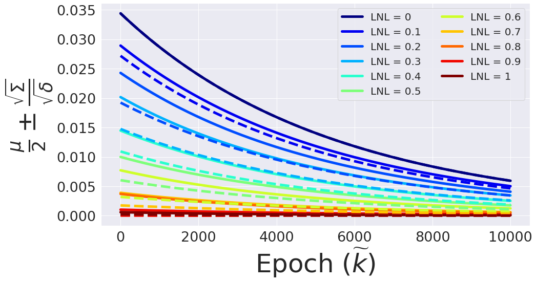
(a)

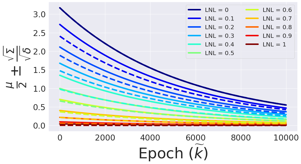
(b)

(c)

(d)

(e)

(f)

Figure 38: The lower (dashed lines) and upper (solid lines) bound terms of Theorem 2 that depend on the label noise level (LNL) are depicted as a function of the number of epochs $\widetilde{k}$, for different hyper-parameter values (the learning rate $\eta$ and $k$) with $\delta=0.05$. The eigenvector projections $p_{i}$ that appear in $\mu$ and $\Sigma$ are computed from the Gram-matrix of $1000$ samples from the MNIST dataset. The resulting values are obtained from an average over $10$ random draws of the label vector y. We observe that both the lower and the upper bounds of Equation (23) are decreasing functions of LNL and of $\widetilde{k}$.

$\eta=10^{-6}$   
$\eta=10^{-3}$

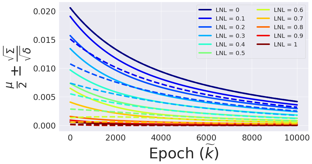
(a)

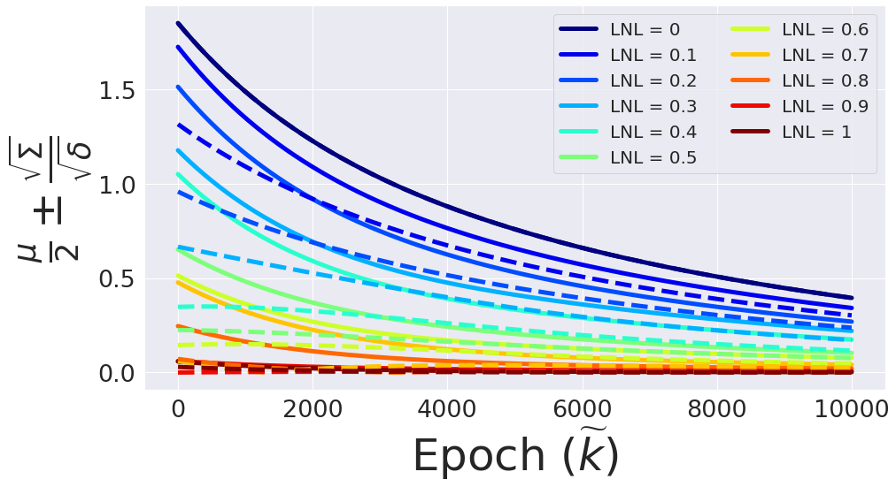
(b)

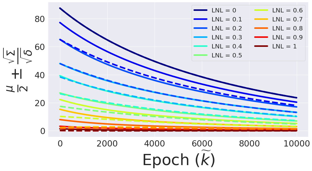
(c)

(d)

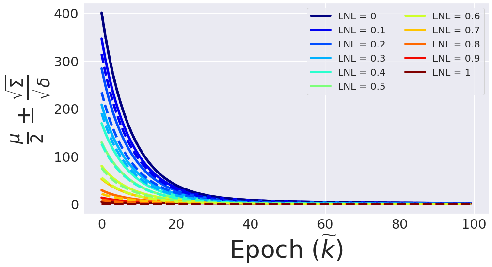
(e)

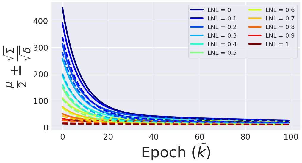
(f)

Figure 39: The lower (dashed lines) and upper (solid lines) bound terms of Theorem 2 that depend on the label noise level (LNL) are depicted as a function of the number of epochs $\widetilde{k}$, for different hyper-parameter values (the learning rate $\eta$ and $k$) with $\delta=0.05$. The eigenvector projections $p_{i}$ that appear in $\mu$ and $\Sigma$ are computed from the Gram-matrix of $1000$ samples from the Fashion-MNIST dataset. The resulting values are obtained from an average over $10$ random draws of the label vector y. We observe that both the lower and the upper bounds of Equation (23) are decreasing functions of LNL and of $\widetilde{k}$.

$\eta=10^{-6}$   
$\eta=10^{-3}$

(a)

(b)

(c)

(d)

(e)

(f)

Figure 40: The lower (dashed lines) and upper (solid lines) bound terms of Theorem 2 that depend on the label noise level (LNL) are depicted as a function of the number of epochs $\widetilde{k}$, for different hyper-parameter values (the learning rate $\eta$ and $k$) with $\delta=0.05$. The eigenvector projections $p_{i}$ that appear in $\mu$ and $\Sigma$ are computed from the Gram-matrix of $1000$ samples from the CIFAR-10 dataset. The resulting values are obtained from an average over $10$ random draws of the label vector y. We observe that both the lower and the upper bounds of Equation (23) are decreasing functions of LNL and of $\widetilde{k}$.

$\eta=10^{-6}$   
$\eta=10^{-3}$

(a)

(b)

(c)

(d)

(e)

(f)

Figure 41: The lower (dashed lines) and upper (solid lines) bound terms of Theorem 2 that depend on the label noise level (LNL) are depicted as a function of the number of epochs $\widetilde{k}$, for different hyper-parameter values (the learning rate $\eta$ and $k$) with $\delta=0.05$. The eigenvector projections $p_{i}$ that appear in $\mu$ and $\Sigma$ are computed from the Gram-matrix of $1000$ samples from the SVHN dataset. The resulting values are obtained from an average over $10$ random draws of the label vector y. We observe that both the lower and the upper bounds of Equation (23) are decreasing functions of LNL and of $\widetilde{k}$.

References

- Akhtar and Mian [2018] N. Akhtar and A. Mian. Threat of adversarial attacks on deep learning in computer vision: A survey. Ieee Access, 6:14410–14430, 2018.
- Allen-Zhu et al. [2018] Z. Allen-Zhu, Y. Li, and Y. Liang. Learning and generalization in overparameterized neural networks, going beyond two layers. arXiv preprint arXiv:1811.04918, 2018.
- Andreassen et al. [2021] A. Andreassen, Y. Bahri, B. Neyshabur, and R. Roelofs. The evolution of out-of-distribution robustness throughout fine-tuning. arXiv preprint arXiv:2106.15831, 2021.
- Arora et al. [2019] S. Arora, S. Du, W. Hu, Z. Li, and R. Wang. Fine-grained analysis of optimization and generalization for overparameterized two-layer neural networks. In International Conference on Machine Learning, pages 322–332. PMLR, 2019.
- Arpit et al. [2017] D. Arpit, S. Jastrzębski, N. Ballas, D. Krueger, E. Bengio, M. S. Kanwal, T. Maharaj, A. Fischer, A. Courville, Y. Bengio, et al. A closer look at memorization in deep networks. In International Conference on Machine Learning, pages 233–242. PMLR, 2017.
- Athalye et al. [2018] A. Athalye, N. Carlini, and D. Wagner. Obfuscated gradients give a false sense of security: Circumventing defenses to adversarial examples. In International conference on machine learning, pages 274–283. PMLR, 2018.
- Baldock et al. [2021] R. Baldock, H. Maennel, and B. Neyshabur. Deep learning through the lens of example difficulty. Advances in Neural Information Processing Systems, 34, 2021.
- Bietti and Mairal [2019] A. Bietti and J. Mairal. On the inductive bias of neural tangent kernels. arXiv preprint arXiv:1905.12173, 2019.
- Brown et al. [2021] G. Brown, M. Bun, V. Feldman, A. Smith, and K. Talwar. When is memorization of irrelevant training data necessary for high-accuracy learning? In Proceedings of the 53rd Annual ACM SIGACT Symposium on Theory of Computing, pages 123–132, 2021.
- Carlini and Wagner [2017] N. Carlini and D. Wagner. Towards evaluating the robustness of neural networks. In 2017 ieee symposium on security and privacy (sp), pages 39–57. IEEE, 2017.
- Chatterjee [2020] S. Chatterjee. Coherent gradients: An approach to understanding generalization in gradient descent-based optimization. arXiv preprint arXiv:2002.10657, 2020.
- Chatterji et al. [2019] N. S. Chatterji, B. Neyshabur, and H. Sedghi. The intriguing role of module criticality in the generalization of deep networks. arXiv preprint arXiv:1912.00528, 2019.
- Chen et al. [2019] P. Chen, B. B. Liao, G. Chen, and S. Zhang. Understanding and utilizing deep neural networks trained with noisy labels. In International Conference on Machine Learning, pages 1062–1070. PMLR, 2019.
- Chen et al. [2021] P. Chen, J. Ye, G. Chen, J. Zhao, and P.-A. Heng. Robustness of accuracy metric and its inspirations in learning with noisy labels. In Proceedings of the AAAI Conference on Artificial Intelligence, volume 35, pages 11451–11461, 2021.
- Du et al. [2018] S. S. Du, X. Zhai, B. Poczos, and A. Singh. Gradient descent provably optimizes over-parameterized neural networks. arXiv preprint arXiv:1810.02054, 2018.
- Feldman [2020] V. Feldman. Does learning require memorization? a short tale about a long tail. In Proceedings of the 52nd Annual ACM SIGACT Symposium on Theory of Computing, pages 954–959, 2020.
- Feldman and Zhang [2020] V. Feldman and C. Zhang. What neural networks memorize and why: Discovering the long tail via influence estimation. arXiv preprint arXiv:2008.03703, 2020.
- Frénay and Verleysen [2013] B. Frénay and M. Verleysen. Classification in the presence of label noise: a survey. IEEE transactions on neural networks and learning systems, 25(5):845–869, 2013.
- Garg et al. [2021a] S. Garg, S. Balakrishnan, J. Z. Kolter, and Z. C. Lipton. Ratt: Leveraging unlabeled data to guarantee generalization. arXiv preprint arXiv:2105.00303, 2021a.
- Garg et al. [2021b] S. Garg, S. Balakrishnan, Z. C. Lipton, B. Neyshabur, and H. Sedghi. Leveraging unlabeled data to predict out-of-distribution performance. In NeurIPS 2021 Workshop on Distribution Shifts: Connecting Methods and Applications, 2021b.
- Goodfellow et al. [2014] I. J. Goodfellow, J. Shlens, and C. Szegedy. Explaining and harnessing adversarial examples. arXiv preprint arXiv:1412.6572, 2014.
- Gu and Tresp [2019] J. Gu and V. Tresp. Neural network memorization dissection. arXiv preprint arXiv:1911.09537, 2019.
- Guo et al. [2017] C. Guo, G. Pleiss, Y. Sun, and K. Q. Weinberger. On calibration of modern neural networks. In International Conference on Machine Learning, pages 1321–1330. PMLR, 2017.
- Guo et al. [2019] C. Guo, J. Gardner, Y. You, A. G. Wilson, and K. Weinberger. Simple black-box adversarial attacks. In International Conference on Machine Learning, pages 2484–2493. PMLR, 2019.
- Han et al. [2020] B. Han, Q. Yao, T. Liu, G. Niu, I. W. Tsang, J. T. Kwok, and M. Sugiyama. A survey of label-noise representation learning: Past, present and future. arXiv preprint arXiv:2011.04406, 2020.
- Harutyunyan et al. [2020] H. Harutyunyan, K. Reing, G. Ver Steeg, and A. Galstyan. Improving generalization by controlling label-noise information in neural network weights. In International Conference on Machine Learning, pages 4071–4081. PMLR, 2020.
- He et al. [2016a] K. He, X. Zhang, S. Ren, and J. Sun. Deep residual learning for image recognition. In Proceedings of the IEEE conference on computer vision and pattern recognition, pages 770–778, 2016a.
- He et al. [2016b] K. He, X. Zhang, S. Ren, and J. Sun. Identity mappings in deep residual networks. In European conference on computer vision, pages 630–645. Springer, 2016b.
- Howard et al. [2017] A. G. Howard, M. Zhu, B. Chen, D. Kalenichenko, W. Wang, T. Weyand, M. Andreetto, and H. Adam. Mobilenets: Efficient convolutional neural networks for mobile vision applications. arXiv preprint arXiv:1704.04861, 2017.
- Hu et al. [2018] J. Hu, L. Shen, and G. Sun. Squeeze-and-excitation networks. In Proceedings of the IEEE conference on computer vision and pattern recognition, pages 7132–7141, 2018.
- Huang et al. [2017] G. Huang, Z. Liu, L. Van Der Maaten, and K. Q. Weinberger. Densely connected convolutional networks. In Proceedings of the IEEE conference on computer vision and pattern recognition, pages 4700–4708, 2017.
- Iandola et al. [2016] F. N. Iandola, S. Han, M. W. Moskewicz, K. Ashraf, W. J. Dally, and K. Keutzer. Squeezenet: Alexnet-level accuracy with 50x fewer parameters and< 0.5 mb model size. arXiv preprint arXiv:1602.07360, 2016.
- Jacot et al. [2018] A. Jacot, F. Gabriel, and C. Hongler. Neural tangent kernel: Convergence and generalization in neural networks. arXiv preprint arXiv:1806.07572, 2018.
- Jastrzebski et al. [2020] S. Jastrzebski, M. Szymczak, S. Fort, D. Arpit, J. Tabor, K. Cho, and K. Geras. The break-even point on optimization trajectories of deep neural networks. arXiv preprint arXiv:2002.09572, 2020.
- [35] A. Q. Jiang and L. S. C. L. Y. Gal. Can network flatness explain the training speed-generalisation connection?
- Krizhevsky et al. [2012] A. Krizhevsky, I. Sutskever, and G. E. Hinton. Imagenet classification with deep convolutional neural networks. Advances in neural information processing systems, 25:1097–1105, 2012.
- Krueger et al. [2017] D. Krueger, N. Ballas, S. Jastrzebski, D. Arpit, M. S. Kanwal, T. Maharaj, E. Bengio, A. Fischer, and A. Courville. Deep nets don’t learn via memorization. 2017.
- Lam and Stork [2003] C. P. Lam and D. G. Stork. Evaluating classifiers by means of test data with noisy labels. In IJCAI, volume 3, pages 513–518. Citeseer, 2003.
- Le and Yang [2015] Y. Le and X. Yang. Tiny imagenet visual recognition challenge. CS 231N, 7(7):3, 2015.
- Lee et al. [2019] J. Lee, L. Xiao, S. Schoenholz, Y. Bahri, R. Novak, J. Sohl-Dickstein, and J. Pennington. Wide neural networks of any depth evolve as linear models under gradient descent. Advances in neural information processing systems, 32:8572–8583, 2019.
- Li et al. [2019] J. Li, Y. Wong, Q. Zhao, and M. S. Kankanhalli. Learning to learn from noisy labeled data. In Proceedings of the IEEE/CVF Conference on Computer Vision and Pattern Recognition, pages 5051–5059, 2019.
- Li et al. [2020] J. Li, M. Zhang, K. Xu, J. P. Dickerson, and J. Ba. Noisy labels can induce good representations. arXiv preprint arXiv:2012.12896, 2020.
- Li et al. [2021] J. Li, M. Zhang, K. Xu, J. Dickerson, and J. Ba. How does a neural network’s architecture impact its robustness to noisy labels? Advances in Neural Information Processing Systems, 34, 2021.
- Liu et al. [2020] S. Liu, J. Niles-Weed, N. Razavian, and C. Fernandez-Granda. Early-learning regularization prevents memorization of noisy labels. arXiv preprint arXiv:2007.00151, 2020.
- Lu and He [2022] Y. Lu and W. He. Selc: Self-ensemble label correction improves learning with noisy labels. arXiv preprint arXiv:2205.01156, 2022.
- Lyle et al. [2020] C. Lyle, L. Schut, B. Ru, Y. Gal, and M. van der Wilk. A bayesian perspective on training speed and model selection. arXiv preprint arXiv:2010.14499, 2020.
- Ma et al. [2018] N. Ma, X. Zhang, H.-T. Zheng, and J. Sun. Shufflenet v2: Practical guidelines for efficient cnn architecture design. In Proceedings of the European conference on computer vision (ECCV), pages 116–131, 2018.
- Ma et al. [2020] X. Ma, H. Huang, Y. Wang, S. Romano, S. Erfani, and J. Bailey. Normalized loss functions for deep learning with noisy labels. In ICML, 2020.
- Maennel et al. [2020] H. Maennel, I. Alabdulmohsin, I. Tolstikhin, R. J. Baldock, O. Bousquet, S. Gelly, and D. Keysers. What do neural networks learn when trained with random labels? arXiv preprint arXiv:2006.10455, 2020.
- Nakkiran et al. [2021] P. Nakkiran, G. Kaplun, Y. Bansal, T. Yang, B. Barak, and I. Sutskever. Deep double descent: Where bigger models and more data hurt. Journal of Statistical Mechanics: Theory and Experiment, 2021(12):124003, 2021.
- Netzer et al. [2011] Y. Netzer, T. Wang, A. Coates, A. Bissacco, B. Wu, and A. Y. Ng. Reading digits in natural images with unsupervised feature learning. 2011.
- Neyshabur et al. [2020] B. Neyshabur, H. Sedghi, and C. Zhang. What is being transferred in transfer learning? Advances in neural information processing systems, 33:512–523, 2020.
- Nguyen et al. [2019] D. T. Nguyen, C. K. Mummadi, T. P. N. Ngo, T. H. P. Nguyen, L. Beggel, and T. Brox. Self: Learning to filter noisy labels with self-ensembling. arXiv preprint arXiv:1910.01842, 2019.
- Nigam et al. [2020] N. Nigam, T. Dutta, and H. P. Gupta. Impact of noisy labels in learning techniques: a survey. In Advances in data and information sciences, pages 403–411. Springer, 2020.
- Papernot et al. [2016a] N. Papernot, P. McDaniel, and I. Goodfellow. Transferability in machine learning: from phenomena to black-box attacks using adversarial samples. arXiv preprint arXiv:1605.07277, 2016a.
- Papernot et al. [2016b] N. Papernot, P. McDaniel, S. Jha, M. Fredrikson, Z. B. Celik, and A. Swami. The limitations of deep learning in adversarial settings. In 2016 IEEE European symposium on security and privacy (EuroS&P), pages 372–387. IEEE, 2016b.
- Patel and Sastry [2021] D. Patel and P. Sastry. Memorization in deep neural networks: Does the loss function matter? In Pacific-Asia Conference on Knowledge Discovery and Data Mining, pages 131–142. Springer, 2021.
- Pedraza et al. [2021] A. Pedraza, O. Deniz, and G. Bueno. On the relationship between generalization and robustness to adversarial examples. Symmetry, 13(5):817, 2021.
- Pereyra et al. [2017] G. Pereyra, G. Tucker, J. Chorowski, Ł. Kaiser, and G. Hinton. Regularizing neural networks by penalizing confident output distributions. arXiv preprint arXiv:1701.06548, 2017.
- Pleiss et al. [2020] G. Pleiss, T. Zhang, E. Elenberg, and K. Q. Weinberger. Identifying mislabeled data using the area under the margin ranking. Advances in Neural Information Processing Systems, 33:17044–17056, 2020.
- Pulastya et al. [2021] V. Pulastya, G. Nuti, Y. K. Atri, and T. Chakraborty. Assessing the quality of the datasets by identifying mislabeled samples. In Proceedings of the 2021 IEEE/ACM International Conference on Advances in Social Networks Analysis and Mining, pages 18–22, 2021.
- Radosavovic et al. [2020] I. Radosavovic, R. P. Kosaraju, R. Girshick, K. He, and P. Dollár. Designing network design spaces. In Proceedings of the IEEE/CVF Conference on Computer Vision and Pattern Recognition, pages 10428–10436, 2020.
- Rahaman et al. [2019] N. Rahaman, A. Baratin, D. Arpit, F. Draxler, M. Lin, F. Hamprecht, Y. Bengio, and A. Courville. On the spectral bias of neural networks. In International Conference on Machine Learning, pages 5301–5310. PMLR, 2019.
- Ru et al. [2021] R. Ru, C. Lyle, L. Schut, M. Fil, M. van der Wilk, and Y. Gal. Speedy performance estimation for neural architecture search. Advances in Neural Information Processing Systems, 34, 2021.
- Sandler et al. [2018] M. Sandler, A. Howard, M. Zhu, A. Zhmoginov, and L.-C. Chen. Mobilenetv2: Inverted residuals and linear bottlenecks. In Proceedings of the IEEE conference on computer vision and pattern recognition, pages 4510–4520, 2018.
- Simonyan and Zisserman [2014] K. Simonyan and A. Zisserman. Very deep convolutional networks for large-scale image recognition. arXiv preprint arXiv:1409.1556, 2014.
- Song et al. [2019] H. Song, M. Kim, and J.-G. Lee. SELFIE: Refurbishing unclean samples for robust deep learning. In ICML, 2019.
- Song et al. [2020a] H. Song, M. Kim, D. Park, Y. Shin, and J.-G. Lee. Learning from noisy labels with deep neural networks: A survey. arXiv preprint arXiv:2007.08199, 2020a.
- Song et al. [2020b] J. Song, Y. Dauphin, M. Auli, and T. Ma. Robust and on-the-fly dataset denoising for image classification. In European Conference on Computer Vision, pages 556–572. Springer, 2020b.
- Stutz et al. [2019] D. Stutz, M. Hein, and B. Schiele. Disentangling adversarial robustness and generalization. In Proceedings of the IEEE/CVF Conference on Computer Vision and Pattern Recognition, pages 6976–6987, 2019.
- Szegedy et al. [2013] C. Szegedy, W. Zaremba, I. Sutskever, J. Bruna, D. Erhan, I. Goodfellow, and R. Fergus. Intriguing properties of neural networks. arXiv preprint arXiv:1312.6199, 2013.
- Szegedy et al. [2015] C. Szegedy, W. Liu, Y. Jia, P. Sermanet, S. Reed, D. Anguelov, D. Erhan, V. Vanhoucke, and A. Rabinovich. Going deeper with convolutions. In Proceedings of the IEEE conference on computer vision and pattern recognition, pages 1–9, 2015.
- Tan and Le [2019] M. Tan and Q. Le. Efficientnet: Rethinking model scaling for convolutional neural networks. In International Conference on Machine Learning, pages 6105–6114. PMLR, 2019.
- Tsipras et al. [2018] D. Tsipras, S. Santurkar, L. Engstrom, A. Turner, and A. Madry. Robustness may be at odds with accuracy. arXiv preprint arXiv:1805.12152, 2018.
- Wei et al. [2021] J. Wei, Z. Zhu, H. Cheng, T. Liu, G. Niu, and Y. Liu. Learning with noisy labels revisited: A study using real-world human annotations. arXiv preprint arXiv:2110.12088, 2021.
- Wei et al. [2022] J. Wei, Z. Zhu, H. Cheng, T. Liu, G. Niu, and Y. Liu. Learning with noisy labels revisited: A study using real-world human annotations. In International Conference on Learning Representations, 2022.
- Xia et al. [2020] X. Xia, T. Liu, B. Han, N. Wang, M. Gong, H. Liu, G. Niu, D. Tao, and M. Sugiyama. Part-dependent label noise: Towards instance-dependent label noise. Advances in Neural Information Processing Systems, 33:7597–7610, 2020.
- Xia et al. [2021] X. Xia, T. Liu, B. Han, C. Gong, N. Wang, Z. Ge, and Y. Chang. Robust early-learning: Hindering the memorization of noisy labels. In ICLR, 2021.
- Xiao et al. [2017] H. Xiao, K. Rasul, and R. Vollgraf. Fashion-mnist: a novel image dataset for benchmarking machine learning algorithms. arXiv preprint arXiv:1708.07747, 2017.
- Xiao et al. [2015] T. Xiao, T. Xia, Y. Yang, C. Huang, and X. Wang. Learning from massive noisy labeled data for image classification. In Proceedings of the IEEE conference on computer vision and pattern recognition, pages 2691–2699, 2015.
- Xie et al. [2017] S. Xie, R. Girshick, P. Dollár, Z. Tu, and K. He. Aggregated residual transformations for deep neural networks. In Proceedings of the IEEE conference on computer vision and pattern recognition, pages 1492–1500, 2017.
- Xu et al. [2019a] Z.-Q. J. Xu, Y. Zhang, T. Luo, Y. Xiao, and Z. Ma. Frequency principle: Fourier analysis sheds light on deep neural networks. arXiv preprint arXiv:1901.06523, 2019a.
- Xu et al. [2019b] Z.-Q. J. Xu, Y. Zhang, and Y. Xiao. Training behavior of deep neural network in frequency domain. In International Conference on Neural Information Processing, pages 264–274. Springer, 2019b.
- Yang et al. [2020] Y.-Y. Yang, C. Rashtchian, H. Zhang, R. Salakhutdinov, and K. Chaudhuri. A closer look at accuracy vs. robustness. arXiv preprint arXiv:2003.02460, 2020.
- Yin et al. [2019] D. Yin, R. Kannan, and P. Bartlett. Rademacher complexity for adversarially robust generalization. In International conference on machine learning, pages 7085–7094. PMLR, 2019.
- Yu et al. [2018] F. Yu, D. Wang, E. Shelhamer, and T. Darrell. Deep layer aggregation. In Proceedings of the IEEE conference on computer vision and pattern recognition, pages 2403–2412, 2018.
- Zhang et al. [2019a] C. Zhang, S. Bengio, and Y. Singer. Are all layers created equal? arXiv preprint arXiv:1902.01996, 2019a.
- Zhang et al. [2021a] C. Zhang, S. Bengio, M. Hardt, B. Recht, and O. Vinyals. Understanding deep learning (still) requires rethinking generalization. Communications of the ACM, 64(3):107–115, 2021a.
- Zhang et al. [2017] H. Zhang, M. Cisse, Y. N. Dauphin, and D. Lopez-Paz. mixup: Beyond empirical risk minimization. arXiv preprint arXiv:1710.09412, 2017.
- Zhang et al. [2019b] H. Zhang, Y. Yu, J. Jiao, E. Xing, L. El Ghaoui, and M. Jordan. Theoretically principled trade-off between robustness and accuracy. In International Conference on Machine Learning, pages 7472–7482. PMLR, 2019b.
- Zhang et al. [2016] J. Zhang, X. Wu, and V. S. Sheng. Learning from crowdsourced labeled data: a survey. Artificial Intelligence Review, 46(4):543–576, 2016.
- Zhang et al. [2019c] J. Zhang, E. Barr, B. Guedj, M. Harman, and J. Shawe-Taylor. Perturbed model validation: A new framework to validate model relevance. 2019c.
- Zhang et al. [2020] X. Zhang, H. Xiong, and D. Wu. Rethink the connections among generalization, memorization and the spectral bias of dnns. arXiv preprint arXiv:2004.13954, 2020.
- Zhang et al. [2021b] X. Zhang, P. Hou, X. Zhang, and J. Sun. Neural architecture search with random labels. In Proceedings of the IEEE/CVF Conference on Computer Vision and Pattern Recognition, pages 10907–10916, 2021b.
- Zhu et al. [2021] Z. Zhu, Z. Dong, H. Cheng, and Y. Liu. A good representation detects noisy labels. arXiv preprint arXiv:2110.06283, 2021.
- Ziyin et al. [2020] L. Ziyin, B. Chen, R. Wang, P. P. Liang, R. Salakhutdinov, L.-P. Morency, and M. Ueda. Learning not to learn in the presence of noisy labels. arXiv preprint arXiv:2002.06541, 2020.