Low-Bitrate Redundancy Coding of Speech Using a Rate-Distortion-Optimized Variational Autoencoder

Abstract

Robustness to packet loss is one of the main ongoing challenges in real-time speech communication. Deep packet loss concealment (PLC) techniques have recently demonstrated improved quality compared to traditional PLC. Despite that, all PLC techniques hit fundamental limitations when too much acoustic information is lost. To reduce losses in the first place, data is commonly sent multiple times using various redundancy mechanisms. We propose a neural speech coder specifically optimized to transmit a large amount of overlapping redundancy at a very low bitrate, up to 50x redundancy using less than 32 kb/s. Results show that the proposed redundancy is more effective than the existing Opus codec redundancy, and that the two can be combined for even greater robustness.

Index Terms— neural speech coding, audio redundancy, variational autoencoder

1 Introduction

In the past few years, deep neural network techniques have significantly improved the state of the art in speech processing. In particular, neural speech coding has significantly increased the quality of very low bitrate speech transmission [1, 2, 3]. Recently, the Interspeech 2022 Audio Deep Packet Loss Concealment (PLC) Challenge [4] demonstrated that neural techniques can improve over classical concealment techniques, paving the way for more reliable speech transmission over the Internet. At the same time, no matter how advanced, PLC techniques are fundamentally limited in their ability to conceal losses since they cannot (and should not) predict missing phonemes/words.

A well-known method for further increasing loss robustness over packet networks is to transmit redundant audio data (RED) [5]. The Opus codec [6] defines a low-bitrate redundancy (LBRR) option to reduce the cost of redundancy by including in each packet a lower bit-rate copy of the previous packet’s contents. Variants and combinations of these methods have been investigated, but there are limits to how far these can scale given that significantly increasing the bitrate can lead to more losses.

In this work, we propose a deep redundancy (DRED) mechanism based on speech coding techniques specifically optimized for coding redundant audio information. Efficiency is achieved by using a continuously-operating recurrent encoder with a decoder running backward in time (Section 2). Our approach is based on a rate-distortion-optimized variational autoencoder (RDO-VAE) that quantizes a Laplace-distributed latent space (Section 3). Whereas typical wideband speech might be transmitted at 24 kb/s with an additional 16 kb/s to provide one frame of redundancy, we demonstrate that DRED is capable of encoding up to 1 second of redundancy in each 20-ms packet (i.e., 50x redundancy) by adding a total of only 31 kb/s. Results in Section 4 show that the proposed approach significantly improves loss robustness, in a way that effectively complements traditional redundancy coding methods.

2 Deep Redundancy (DRED) Overview

Most speech codecs in use today encode audio in 20-ms frames, with each frame typically being sent in a separate packet over the Internet. When any packet is lost, the corresponding audio is lost and has to be filled by a PLC algorithm. The Opus LBRR option makes it possible for packet number $n$ to include the contents of both frames $n$ and $n-1$, with the latter being encoded at a slightly lower bitrate. Effectively, packets each contains 40-ms of audio despite being sent at a 20-ms interval. When LBRR is enabled, a single packet loss does not cause any audio frame to be completely lost, which can improve the quality in difficult network conditions. Unfortunately, losses are rarely uniformly distributed, and LBRR has limited impact on long loss bursts. While more frames could be coded as part of each packet, it would cause the bitrate to go up significantly. For that reason, we propose an efficient neural coding technique that makes it possible to include a large amount of redundancy without a large increase in bitrate.

The signal-level architecture for the proposed redundancy coding is derived from our previous work on packet loss concealment, where a vocoder is used to fill in the missing frames using acoustic features produced by a predictor (Section 4.3 of  [7]). In this work, we replace the acoustic feature predictor by an encoder and decoder that transmit a lossy approximation of the ground-truth features. Although we only discuss redundant audio coding here, our architecture makes it easy to integrate redundancy coding with PLC.

2.1 Constraints and hypotheses

Since the purpose of this work is to improve robustness to packet loss, an obvious constraint is to avoid any prediction across different packets. That being said, within each packet, any amount of prediction is allowed since we assume that a packet either arrives uncorrupted, or does not arrive at all. Additionally, since the same frame information is encoded in multiple packets, we do not wish to re-encode each packet from scratch, but rather have a continuously-running encoder from which we extract overlapping encoded frames. On the decoder side, since short losses are more likely than very long ones, it is desirable to be able to decode only the last few frames of speech without having to decode the entire packet.

To maximize efficiency, we can take advantage of (variable-length) entropy coding. Even if a constant bitrate was ultimately desired, that could easily be achieved by varying the duration of the redundancy. At last, we can also take advantage of variable encoding quality as a function of the timestamp within the redundant packet. After all, more recent packets are expected to be used more often, so they deserve to be coded at a higher quality.

Although there are many different types of neural vocoders, we propose to use an auto-regressive vocoder, as it allows for seamless transitions between regular coded audio and low-bitrate redundant audio without the use of cross-fading. Although in this work we use LPCNet [8] due to its low complexity, any other auto-regressive vocoder would also be applicable.

2.2 Proposed architecture

There are generally two methods for improving coding efficiency: prediction and transforms. The proposed algorithm leverages both methods. In the context of neural coding, grouping input feature vectors together enables the encoder to infer an efficient non-linear transform of its input. For prediction, we use a recurrent neural network (RNN) architecture, but to achieve the computational goals listed above, we make the encoder RNN run forward in a continuous manner, while making the decoder RNN run backward in time, from the most recent packet encoded. To ensure that the decoder achieves sufficient quality on the first (most recent) packet, the encoder also codes an initial state (IS). Although the encoder needs to produce such an IS on every frame, only one is included in each redundancy packet.

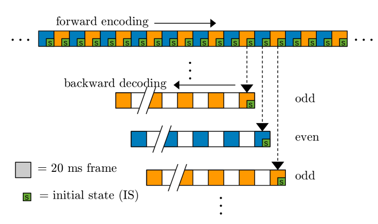
Fig. 1: Overview of the encoding and decoding process. For each 20-ms frame, the encoder processes two 10-ms feature vectors and produces an encoded latent vector (shown in orange or blue), as well as an initial state (IS). Although latent vectors are produced every 20 ms, they each contain sufficient information to reconstruct 40 ms of audio. The encoded stream is split into overlapping redundancy packets. Each packet to be sent contains a single IS (for the latest frame), as well as half of the latent vectors (even or odd) spanning the desired redundancy duration.

Even though our network operates on 20-ms frames, the underlying 20-dimensional LPCNet feature vectors are computed on a 10-ms interval. For that reason we group feature vectors in pairs – equivalent to a 20-ms non-linear transform. To further increase the effective transform size while still producing a redundancy packet every 20 ms, we use an output stride. The process is illustrated for a stride of 2 in Fig. 1 – resulting in each output vector representing 40 ms of speech – but it can easily scale to larger strides.

3 Rate-Distortion-Optimized VAE

As stated above, our goal is to compress each redundancy packet as efficiently as possible. Although VQ-VAE [9] has been a popular choice for neural speech coding [10, 11], in this work we avoid its large fixed-size codebooks and investigate other variational auto-encoders (VAE) [12]. Our approach is instead inspired from recent work in VAE-based image coding [13, 14] combining scalar quantization with entropy coding.

We propose a rate-distortion-optimized VAE (RDO-VAE) that directly minimizes a rate-distortion loss function. From a sequence of input vectors $\mathbf{x}\in\mathbb{R}^{L}$, the RDO-VAE produces an output $\tilde{\mathbf{x}}\in\mathbb{R}^{L}$ by going through a sequence of quantized latent vectors $\mathbf{z}_{q}\in\mathbb{Z}^{M}$, minimizing the loss function

$$\mathcal{L}=D\left(\tilde{\mathbf{x}},\mathbf{x}\right)+\lambda H\left(\mathbf{z}_{q}\right)\ ,$$ (1)

where $D\left(\cdot,\cdot\right)$ is the distortion loss, and $H\left(\cdot\right)$ denotes the entropy. The Lagrange multiplier $\lambda$ effectively controls the target rate, with a higher value leading to a lower rate. The high-level encoding and decoding process is illustrated in Fig. 2.

Because the latent vectors $\mathbf{z}_{q}$ are quantized, neither $D\left(\cdot,\cdot\right)$ nor $H\left(\cdot\right)$ in (1) are differentiable. For the distortion, a common way around the problem is to use the straight-through estimator [9, 15]. More recently, various combinations involving “soft” quantization – through the addition of uniformly distributed noise – have been shown to produce better results [13, 14]. In this work, we choose to use a weighted average of the soft and straight-through (hard quantization) distortions.

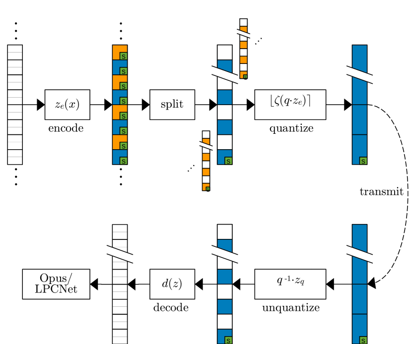
Fig. 2: Encoding and decoding process. The encoder produces latent vectors and initial states from LPCNet features. The vectors are split into overlapping redundancy packets and then quantized using a variable resolution (the same vector can be quantized at different rates depending on its position). At the receiver, the redundancy packets are entropy-decoded and scaled back (unquantized) to recover the latent vectors. Those are then decoded to produce 10-ms LPCNet feature vectors that can be used to synthesize audio in place of the missing Opus packets. The redundancy decoding process happens only on-demand such that no computation occurs when there is no loss.

3.1 Rate Estimator

We use the Laplace distribution to model the latent space because it is easy to manipulate and is relatively robust to probability modeling mismatches. Since we can consider the rate of each variable independently, let $z_{e}$ and $z_{q}$ represent one component of the unquantized ($\mathbf{z}_{e}$) and quantized ($\mathbf{z}_{q}$) vectors, respectively. The continuous Laplace distribution is given by:

$$p\left(z_{e}\right)=-\frac{\log r}{2}r^{\left|z_{e}\right|}\ ,$$ (2)

where $r$ is related to the standard deviation $\sigma$ by $r=e^{-\sqrt{2}/\sigma}$.

An efficient way of quantizing a Laplace-distributed variable [16] is to use a fixed quantization step size, except around zero, where all values of $q_{e}\in\left]-\theta,\theta\right[$ quantize to zero, with $\theta>\frac{1}{2}$ arising from rate-distortion optimization. We describe a quantizer with a step size of one without loss of generality, since we can always scale the input and output to achieve the desired quantization resolution. We thus define the quantizer as:

$$z_{q}=Q_{\theta}\left(z_{e}\right)=\mathrm{sgn}\left(z_{e}\right)\left\lfloor\max\left(\left|z_{e}\right|+1-\theta,\ 0\right)\right\rfloor\ ,$$ (3)

where $\mathrm{sgn}\left(\cdot\right)$ denotes the sign function. In the special case $\theta=1/2$, we simply round to the nearest integer (ignoring ties).

The discrete pdf of a quantized Laplace distribution is

$$P\left(z_{q}\right)=\begin{cases}1-r^{\theta}&z_{q}=0\\ \frac{1}{2}\left(1-r\right)r^{\left|z_{q}\right|+\theta-1}&z_{q}\neq 0\end{cases}\ .$$ (4)

Since its entropy, $H\left(z_{q}\right)=\mathbb{E}\left[-\log_{2}P\left(z_{q}\right)\right]$, is not differentiable with respect to $z_{e}$, we must find a way to backpropagate the gradient. We find that using the straight-through estimator for the rate results in very poor convergence, with the training loss starting to increase again after a few epochs due to the mismatch between the forward and backward pass of backpropagation.

We seek to use a differentiable rate estimation on the unquantized encoder output. An obvious choice is to use the differential entropy $h\left(z_{e}\right)=\mathbb{E}\left[-\log_{2}p\left(z_{e}\right)\right]$, which achieves better convergence. Unfortunately, the differential entropy tends towards $-\infty$ when $p\left(z_{e}\right)$ becomes degenerate as $r\rightarrow 0$, which can cause many low-variance latent variables to collapse to zero. Instead, we use the continuous $z_{e}$ with the entropy of the discrete distribution $H\left(z_{e}\right)=\mathbb{E}\left[-\log_{2}P\left(z_{e}\right)\right]$. We further simplify the rate estimate by selecting the implicit threshold value $\theta=\log_{r}\left(2r/\left(1+r\right)\right)$, chosen such that $z_{e}=0$ is no longer a special case, resulting in

$$H\left(z_{e}\right)=-\log_{2}\frac{1-r}{1+r}-\mathbb{E}\left[\left|z_{e}\right|\right]\log_{2}r\ .$$ (5)

In the degenerate case where $r\rightarrow 0$ (and thus $z_{e}=0$), we have $H\left(z_{e}\right)=0$, which is the desired behavior. An advantage of using (5) is that any latent dimension that does not sufficiently reduce the distortion to be “worth” its rate naturally becomes degenerate during training. We can thus start with more latent dimensions than needed and let the model decide on the number of useful dimensions. In practice, we find that different values of $\lambda$ result in a different number of non-degenerate pdfs.

3.2 Quantization and Encoding

The dead zone, as defined by the quantizer $Q_{\theta}\left(z\right)$ in (3), needs to be differentiable with respect to both its input parameter $z$ and its width $\theta$. That can be achieved by implementing it as the differentiable function

$$\zeta\left(z\right)=z-\delta\tanh\frac{z}{\delta+\epsilon}\ ,$$ (6)

where $\delta\approx\theta-1/2$ controls the width of the dead zone and $\epsilon=0.1$ avoids training instabilities. The complete quantization process thus becomes

$$z_{q}=\left\lfloor\zeta\left(q_{\lambda}\cdot z_{e}\right)\right\rceil\ ,$$ (7)

where $\left\lfloor\cdot\right\rceil$ denotes rounding to the nearest integer, and $q_{\lambda}$ is the quantizer scale (higher $q_{\lambda}$ leads to higher quality). The quantizer scale $q_{\lambda}$ is learned independently as an embedding matrix for each dimension of the latent space and for each value of the rate-control parameter $\lambda$.

The quantized latent components $z_{q}$ can be entropy-coded [17] using the discrete pdf in (4) parameterized by $r$ and $\theta$. The value of $\theta$ is learned independently of the quantizer dead-zone parameter $\delta$. Also, we learn a different $r$ parameter for the soft and hard quantizers. The value of $\theta$ for the soft quantizer is implicit and thus does not need to be learned, although a learned $\theta$ does not lead to significant rate reduction, which is evidence that the implicit $\theta$ is close to the RD-optimal choice.

On the decoder side, the quantized latent vectors are entropy-decoded and the scaling is undone:

$$z_{d}=q_{\lambda}^{-1}\cdot z_{q}\ .$$ (8)

At last, we need to quantize the IS vector $\mathbf{s}$ to be used by the decoder. Although the encoder produces an IS at every frame, only one IS per redundancy packet needs to be transmitted. Because the IS represents only a small fraction of the information transmitted, we transmit it at a fixed bitrate. We constrain the IS to unit-norm and use an algebraic variant of VQ-VAE based on the pyramid vector quantizer (PVQ) [18], with a spherical codebook defined as

$$S_{N,K}=\left\{\frac{\mathbf{p}}{\left\|\mathbf{p}\right\|}:\mathbf{p}\in\mathbb{Z}^{N}\mathrm{\,and\,}\sum_{i=0}^{N-1}\left|p_{i}\right|=K\right\}\ ,$$ (9)

where $N$ is the dimensionality of the IS and $K$ determines the size (and the rate) of the codebook. The size of codebook $S_{N,K}$ is given by the recurrent expression $V_{N,K}=V_{N-1,K}+V_{N,K-1}+V_{N-1,K-1}$, with $V_{0,K}=0$ for $K>0$ and $V_{N,0}=1$. We use a straight-through gradient estimator for PVQ-VAE training.

3.3 Training

During training, we vary $\lambda$ in such a way as to obtain average rates between 15 and 85 bits per vector. We split the $\lambda$ range into 16 equally-spaced intervals in the log domain. For each interval, we learn independent values for $q$, $\delta$, $\theta$, as well as for the hard and soft versions of the Laplace parameter $r$. To avoid giving too much weight to the low-bitrate cases because of the large $\lambda$ values, we reduce the difference in losses by weighting the total loss values by $1/\sqrt{\lambda}$:

$$\mathcal{L}=\frac{D\left(\tilde{\mathbf{x}},\mathbf{x}\right)}{\sqrt{\lambda}}+\sqrt{\lambda}\sum_{i=0}^{M-1}H\left(z_{e}^{(i)};r_{s}^{(i)}\right)\ .$$ (10)

The loss function $D\left(\cdot,\cdot\right)$ combines mean squared error (MSE) terms for the cepstrum and pitch correlation and an absolute error ($L_{1}$) term for the log-domain pitch.

The large overlap between decoded sequences poses a challenge for the training. Running a large number of overlapping decoders would be computationally challenging. On the other hand, we find that decoding the entire sequence produced by the encoder with a single decoder leads to the model over-fitting to that particular case. We find that encoding 4-second sequences and splitting them into four non-overlapping sequences to be independently decoded leads to acceptable performance and training time.

4 Experiments & Results

Both the RDO-VAE and the LPCNet vocoder are trained independently on 205 hours of 16-kHz speech from a combination of TTS datasets [19, 20, 21, 22, 23, 24, 25, 26, 27] including more than 900 speakers in 34 languages and dialects. The vocoder training is performed as described in [28], except that we explicitly randomize the sign of each training sequence so that the algorithm works for any polarity of the speech signal.

The encoder and decoder networks each consist of 3 gated recurrent unit (GRU) [29] layers, mixed with 6 fully-connected layers and a concatenation skip layer at the end. Each layers has 256 units. We train the RDO-VAE with $M=80$ initial latent dimensions, and observe that between 14 and 29 dimensions (depending on bitrate) are ultimately non-degenerate ($r>0.001$).

We evaluate the proposed neural redundancy mechanism on speech compressed with the Opus codec at 24 kb/s, making the conditions comparable to those occurring on a call over WebRTC. We add 1.04 seconds of neural redundancy in each 20-ms frame transmitted, so that 52 copies of every frame are ultimately transmitted (concealing burst losses up to 1.02 seconds). We vary the rate within each redundancy packet such that the average rates are around 750 b/s for the most recent frame and 375 b/s for the oldest. The average rate over all frames is about 500 b/s, to which we add $\log_{2}V_{N,K}=96\ \mathrm{bits}$ for the PVQ quantized state ($N=24$, $K=82$), resulting in about 620 bits of redundancy per frame, or 31 kb/s of total redundancy.

A real-time C implementation of an updated DRED version operating within the Opus codec is available under an open-source license at https://gitlab.xiph.org/xiph/opus in the exp_dred_icassp branch.

4.1 Complexity

The neural encoder and decoder each have about 2 million weights. The encoder uses each weight once (multiply-add) for each 20-ms frame, resulting in a complexity of 0.2 GFLOPS. The decoder’s complexity varies depending on the loss pattern, but can never average more than one step every 40 ms. That results in a worst-case average decoder complexity of 0.1 GFLOPS, although unlike the case of the encoder, the decoder complexity can have bursts. On the receiver side, the complexity will nonetheless be dominated by the LPCNet vocoder’s 4 GFLOPS complexity.

4.2 Quality

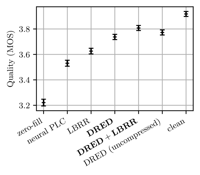
Fig. 3: MOS results, including the 95% confidence intervals. All differences are statistically significant.

We evaluated DRED on the PLC Challenge dataset [4], using the development test set files for both the audio and the recorded packet loss sequences (18.4% average loss rate). The sequences have loss ranging from 20 ms to bursts of up to one second, meaning that the redundancy is able to cover all losses without the need for regular PLC. We compare with the neural PLC results obtained in [7] (no redundancy), as well as with the original Opus LBRR, both alone (requiring PLC) and combined with DRED (the first DRED frame becomes unused). We also include an upper bound where DRED is applied with uncompressed features. We include as anchors both clean/lossless samples and samples where losses are replaced with zeros.

The mean opinion score (MOS) [30] results in Table 3 were obtained using the crowdsourcing methodology described in P.808 [31, 32], where each of the 966 test utterances was evaluated by 15 randomly-selected naive listeners. Listeners were asked to rate samples on an absolute category rating scale from 1 (bad) to 5 (excellent). The results show that DRED significantly outperforms both neural PLC and the existing Opus LBRR. Despite the very low bitrate used for the redundancy, the performance is already close to the uncompressed upper bound, suggesting that the vocoder may already be the performance bottleneck. We also note that LBRR and DRED appear to be complementary, with LBRR being more efficient for short losses and DRED handling long losses.

5 Conclusion

We demonstrate that large amounts of audio redundancy can be efficiently encoded at low bitrate to significantly improve the robustness of a communication system to packet loss. We use a recurrent rate-distortion-optimized VAE to compute and quantize Laplace-distributed latent vectors on a 40-ms interval and transmit overlapping segments of redundancy to the receiver. Results show that the proposed redundancy is more effective than the existing Opus codec redundancy, and that the two can be combined for even greater robustness. As with the Opus LBRR, taking advantage of the proposed DRED requires adaptively increasing the jitter buffer delay. Making optimal trade-offs between loss robustness and delay is still an open question left to be resolved.

References

- [1] W. B. Kleijn, F. SC Lim, A. Luebs, J. Skoglund, F. Stimberg, Q. Wang, and T. C. Walters, “WaveNet based low rate speech coding,” in Proc. International Conference on Acoustics, Speech and Signal Processing (ICASSP), 2018, pp. 676–680.
- [2] J. Klejsa, P. Hedelin, C. Zhou, R. Fejgin, and L. Villemoes, “High-quality speech coding with SampleRNN,” in Proc. International Conference on Acoustics, Speech and Signal Processing (ICASSP), 2019.
- [3] J.-M. Valin and J. Skoglund, “A real-time wideband neural vocoder at 1.6 kb/s using LPCNet,” in Proc. INTERSPEECH, 2019.
- [4] L. Diener, S. Sootla, S. Branets, A. Saabas, R. Aichner, and R. Cutler, “INTERSPEECH 2022 audio deep packet loss concealment challenge,” in Proc. INTERSPEECH, 2022.
- [5] I. Kouvelas, O. Hodson, V. Hardman, M. Handley, J.C. Bolot, A. Vega-Garcia, and S. Fosse-Parisis, “RTP payload for redundant audio data,” RFC 2198, Sept. 1997, https://tools.ietf.org/html/rfc2198.
- [6] J.-M. Valin, K. Vos, and T. B. Terriberry, “Definition of the Opus Audio Codec,” RFC 6716, Sept. 2012, https://tools.ietf.org/html/rfc6716.
- [7] J.-M. Valin, A. Mustafa, C. Montgomery, T.B. Terriberry, M. Klingbeil, P. Smaragdis, and A. Krishnaswamy, “Real-time packet loss concealment with mixed generative and predictive model,” in Proc. INTERSPEECH, 2022.
- [8] J.-M. Valin and J. Skoglund, “LPCNet: Improving neural speech synthesis through linear prediction,” in Proc. International Conference on Acoustics, Speech and Signal Processing (ICASSP), 2019, pp. 5891–5895.
- [9] A. van den Oord, O. Vinyals, and K. Kavukcuoglu, “Neural discrete representation learning,” Advances in neural information processing systems, vol. 30, 2017.
- [10] N. Zeghidour, A. Luebs, A. Omran, J. Skoglund, and M. Tagliasacchi, “SoundStream: An end-to-end neural audio codec,” Trans. on Acoustics, Speech, and Signal Processing, vol. 30, 2021.
- [11] J. Casebeer, V. Vale, U. Isik, J.-M. Valin, R. Giri, and A. Krishnaswamy, “Enhancing into the codec: Noise robust speech coding with vector-quantized autoencoders,” in Proc. International Conference on Acoustics, Speech and Signal Processing (ICASSP), 2021.
- [12] D.P. Kingma and M. Welling, “Auto-encoding variational Bayes,” arxiv:1312.6114, 2013.
- [13] Z. Guo, Z. Zhang, R. Feng, and Z. Chen, “Soft then hard: Rethinking the quantization in neural image compression,” in Proc. ICML, 2021.
- [14] J. Ballé, P. A. Chou, D. Minnen, S. Singh, N. Johnston, E. Agustsson, S.J. Hwang, and G. Toderici, “Nonlinear transform coding,” IEEE Journal of Selected Topics in Signal Processing, vol. 15, no. 2, 2021.
- [15] Y. Bengio, N. Léonard, and A. Courville, “Estimating or propagating gradients through stochastic neurons for conditional computation,” arvix preprint arXiv:1308.3432, 2013.
- [16] G.J. Sullivan, “Efficient scalar quantization of exponential and laplacian random variables,” IEEE Transactions on Information Theory, vol. 42, no. 5, 1996.
- [17] G. Nigel and N. Martin, “Range encoding: An algorithm for removing redundancy from a digitised message,” in Proc. Video and Data Recording Conference, 1979.
- [18] T. Fischer, “A pyramid vector quantizer,” IEEE Trans. on Information Theory, 1986.
- [19] I. Demirsahin, O. Kjartansson, A. Gutkin, and C. Rivera, “Open-source Multi-speaker Corpora of the English Accents in the British Isles,” in Proc. LREC, 2020.
- [20] O. Kjartansson, A. Gutkin, A. Butryna, I. Demirsahin, and C. Rivera, “Open-Source High Quality Speech Datasets for Basque, Catalan and Galician,” in Proc. SLTU and CCURL, 2020.
- [21] K. Sodimana, K. Pipatsrisawat, L. Ha, M. Jansche, O. Kjartansson, P. De Silva, and S. Sarin, “A Step-by-Step Process for Building TTS Voices Using Open Source Data and Framework for Bangla, Javanese, Khmer, Nepali, Sinhala, and Sundanese,” in Proc. SLTU, 2018.
- [22] A. Guevara-Rukoz, I. Demirsahin, F. He, S.-H. C. Chu, S. Sarin, K. Pipatsrisawat, A. Gutkin, A. Butryna, and O. Kjartansson, “Crowdsourcing Latin American Spanish for Low-Resource Text-to-Speech,” in Proc. LREC, 2020.
- [23] F. He, S.-H. C. Chu, O. Kjartansson, C. Rivera, A. Katanova, A. Gutkin, I. Demirsahin, C. Johny, M. Jansche, S. Sarin, and K. Pipatsrisawat, “Open-source Multi-speaker Speech Corpora for Building Gujarati, Kannada, Malayalam, Marathi, Tamil and Telugu Speech Synthesis Systems,” in Proc. LREC, 2020.
- [24] Y. M. Oo, T. Wattanavekin, C. Li, P. De Silva, S. Sarin, K. Pipatsrisawat, M. Jansche, O. Kjartansson, and A. Gutkin, “Burmese Speech Corpus, Finite-State Text Normalization and Pronunciation Grammars with an Application to Text-to-Speech,” in Proc. LREC, 2020.
- [25] D. van Niekerk, C. van Heerden, M. Davel, N. Kleynhans, O. Kjartansson, M. Jansche, and L. Ha, “Rapid development of TTS corpora for four South African languages,” in Proc. INTERSPEECH, 2017.
- [26] A. Gutkin, I. Demirşahin, O. Kjartansson, C. Rivera, and K. Túbọ̀sún, “Developing an Open-Source Corpus of Yoruba Speech,” in Proc. INTERSPEECH, 2020.
- [27] E. Bakhturina, V. Lavrukhin, B. Ginsburg, and Y. Zhang, “Hi-Fi Multi-Speaker English TTS Dataset,” arXiv preprint arXiv:2104.01497, 2021.
- [28] J.-M. Valin, U. Isik, P. Smaragdis, and A. Krishnaswamy, “Neural speech synthesis on a shoestring: Improving the efficiency of LPCNet,” in Proc. International Conference on Acoustics, Speech and Signal Processing (ICASSP), 2022.
- [29] K. Cho, B. Van Merriënboer, D. Bahdanau, and Y. Bengio, “On the properties of neural machine translation: Encoder-decoder approaches,” in Proceedings of Eighth Workshop on Syntax, Semantics and Structure in Statistical Translation, 2014.
- [30] ITU-T, Recommendation P.800: Methods for subjective determination of transmission quality, 1996.
- [31] ITU-T, Recommendation P.808: Subjective evaluation of speech quality with a crowdsourcing approach, 2018.
- [32] B. Naderi and R. Cutler, “An open source implementation of ITU-T recommendation P.808 with validation,” in Proc. INTERSPEECH, 2020.