Abstract

We introduce GAUCHE, a library for GAUssian processes in CHEmistry. Gaussian processes have long been a cornerstone of probabilistic machine learning, affording particular advantages for uncertainty quantification and Bayesian optimisation. Extending Gaussian processes to chemical representations however is nontrivial, necessitating kernels defined over structured inputs such as graphs, strings and bit vectors. By defining such kernels in GAUCHE, we seek to open the door to powerful tools for uncertainty quantification and Bayesian optimisation in chemistry. Motivated by scenarios frequently encountered in experimental chemistry, we showcase applications for GAUCHE in molecular discovery and chemical reaction optimisation. The codebase is made available at https://github.com/leojklarner/gauche

1 Introduction

Early-stage scientific discovery is typically characterised by the limited availability of high-quality experimental data Zhang & Ling (2018); Griffiths et al. (2021a; 2022), leaving lots of knowledge to discover by additional targeted experiments.In contrast, in the big data regime, discovery offers diminishing returns as most knowledge about the space of interest has already been acquired. As such, machine learning methodologies that facilitate discovery in small data regimes such as Bayesian optimisation (BO) Gómez-Bombarelli et al. (2018); Griffiths & Hernández-Lobato (2020); Shields et al. (2021); Du et al. (2022); Griffiths (2023) and active learning (AL) Zhang et al. (2019); Jablonka et al. (2021) have great potential to expedite the rate at which performant molecules, molecular materials, chemical reactions and proteins are discovered.

Currently in molecular machine learning, Bayesian neural networks (BNNs) and deep ensembles are typically used to produce uncertainty estimates for driving BO and AL loops Ryu et al. (2019); Zhang et al. (2019); Hwang et al. (2020); Scalia et al. (2020). For small datasets, however, deep neural networks are often not the model of choice Tom et al. (2022). Notably, certain deep learning experts have voiced a preference for Gaussian processes (GPs) in the small data regime Bengio (2011). Furthermore, for BO, GPs possess particularly advantageous properties; first, they admit exact as opposed to approximate Bayesian inference and second, few of their parameters need to be determined by hand. In the words of Sir David MacKay MacKay et al. (2003),

"Gaussian processes are useful tools for automated tasks where fine tuning for each problem is not possible. We do not appear to sacrifice any performance for this simplicity.”

The iterative model refitting required in BO makes it a prime example of such an automated task. Although BNN surrogates have been trialled for BO Snoek et al. (2015); Springenberg et al. (2016), GPs remain the model of choice as evidenced by the results of the recent NeurIPS Black-Box Optimisation Competition Turner et al. (2021).

Training GPs on molecular inputs, however, is non-trivial. Canonical applications of GPs assume continuous input spaces of low and fixed dimensionality. The most popular molecular input representations are SMILES/SELFIES strings Anderson et al. (1987); Weininger (1988); Krenn et al. (2020), fingerprints Rogers & Hahn (2010); Probst & Reymond (2018); Capecchi et al. (2020) and graphs Duvenaud et al. (2015); Kearnes et al. (2016). Each of these input representations poses problems for GPs. SMILES strings have variable length, fingerprints are high-dimensional and sparse bit vectors, while graphs are also a form of non-continuous input. To construct a GP framework over molecules, GAUCHE provides GPU-based implementations of kernels that operate on molecular inputs, including string, fingerprint and graph kernels. Furthermore, GAUCHE includes support for protein and chemical reaction representations and interfaces with the GPyTorch Gardner et al. (2018) and BoTorch Balandat et al. (2020) libraries to facilitate usage for advanced probabilistic modelling and BO.

Concretely, our contributions may be summarised as:

1. We propose a GP framework for molecules and chemical reactions.

2. We provide an open-source, GPU-enabled library building on GPyTorch Gardner et al. (2018), BoTorch Balandat et al. (2020) and RDKit Landrum (2013).

3. We extend the use of black box graph kernels from GraKel Siglidis et al. (2020) to GP regression via a GPyTorch interface, along with a set of graph kernels implemented in native GPyTorch to enable optimisation of the graph kernel hyperparameters under the marginal likelihood.

4. We conduct benchmark experiments evaluating the utility of the GP framework on regression, uncertainty quantification and BO.

GAUCHE includes tutorials to guide users through the tasks considered in this paper and is made available at https://github.com/leojklarner/gauche.

2 Background

2.1 Gaussian Processes

Notation:

$\mathbf{X}\in\mathbb{R}^{n\times d}$ is a design matrix of $n$ training examples of dimension $d$. A given row $i$ of the design matrix contains a training molecule’s representation $\mathbf{x}_{i}$. A GP is specified by a mean function, $m(\mathbf{x})=\mathbb{E}[f(\mathbf{x})]$ and a covariance function $k(\mathbf{x},\mathbf{x^{\prime}})=\mathbb{E}[(f(\mathbf{x})-m(\mathbf{x}))(f(\mathbf{x^{\prime}})-m(\mathbf{x}))]$. $K_{\theta}(\mathbf{X},\mathbf{X})$ is a kernel matrix where entries are computed by the kernel function as $[K]_{ij}=k(\mathbf{x}_{i},\mathbf{x}_{j})$. $\theta$ represents the set of kernel hyperparameters. The GP specifies the full distribution over the function $f$ to be modelled as

$$f(\mathbf{x})\sim\mathcal{GP}\big{(}m(\mathbf{x}),k(\mathbf{x},\mathbf{x^{\prime}})\big{)}.$$

Prediction:

At test locations $\mathbf{\mathbf{X}_{*}}$ the GP returns a predictive mean, $\mathbf{\bar{f_{*}}}=K(\mathbf{\mathbf{X}_{*}},\mathbf{X})[K(\mathbf{X},\mathbf{X})+\sigma_{y}^{2}I]^{-1}\mathbf{y}$, and a predictive uncertainty $\text{cov}(\mathbf{f_{*}})=K(\mathbf{X_{*}},\mathbf{X_{*}})-K(\mathbf{X_{*}},\mathbf{X})[K(\mathbf{X},\mathbf{X})+\sigma_{y}^{2}I]^{-1}K(\mathbf{X},\mathbf{X_{*}}).$

Kernels:

The choice of kernel is an important inductive bias for the properties of the function being modelled. A common choice for continuous input domains is the radial basis function kernel

$$k_{\text{RBF}}(\mathbf{x},\mathbf{x^{\prime}})=\sigma_{f}^{2}\exp\bigg{(}\frac{-||\mathbf{x}-\mathbf{x}^{\prime}||_{2}^{2}}{2\ell^{2}}\bigg{)},$$

where $\sigma_{f}^{2}$ is the signal amplitude hyperparameter (vertical lengthscale) and $\ell$ is the (horizontal) lengthscale hyperparameter. The symbol $\theta$, introduced previously, is used to represent the set of kernel hyperparameters. For molecules, bespoke kernel functions need to be defined for structured input spaces.

GP Training:

Hyperparameters for GPs comprise kernel hyperparameters, $\theta$, in addition to the likelihood noise, $\sigma_{y}^{2}$. These hyperparameters are chosen by optimising an objective function known as the negative log marginal likelihood (NLML)

$$\log p(\mathbf{y}|\mathbf{X},\theta)= \underbrace{-\frac{1}{2}\mathbf{y}^{\top}(K_{\theta}(\mathbf{X},\mathbf{X})+\sigma_{y}^{2}I)^{-1}\mathbf{y}}_{\text{encourages fit with data}}$$

$$\underbrace{-\frac{1}{2}\log|K_{\theta}(\mathbf{X},\mathbf{X})+\sigma_{y}^{2}I|}_{\text{controls model capacity}}-\frac{N}{2}\log(2\pi).$$

$I\sigma_{y}^{2}$ represents the variance of i.i.d. Gaussian noise on the observations $\mathbf{y}$. The NLML embodies Occam’s razor for Bayesian model selection Rasmussen & Ghahramani (2001) in favouring models that fit the data without being overly complex.

2.2 Bayesian Optimisation

In molecular discovery campaigns we are typically interested in solving problems of the form

$$\mathbf{x}^{\star}=\arg\max_{\mathbf{x}\in\mathcal{X}}f(\mathbf{x}),$$

where $f(\cdot):\mathcal{X}\rightarrow\mathbb{R}$ is an expensive black-box function over a structured input domain $\mathcal{X}$. In our example setting the structured input domain consists of a set of molecular representations (graphs, strings, bit vectors) and the expensive black-box function is a property of interest for a given molecule that we wish to optimise. Bayesian optimisation (BO) (Kushner, 1963; Močkus, 1975; Zhilinskas, 1975; Jones et al., 1998; Brochu et al., 2010; Grosnit et al., 2020) is a data-efficient methodology for determining $\mathbf{x}^{\star}$. BO operates sequentially by selecting input locations at which to query the black-box function $f$ with the aim of identifying the optimum in as few queries as possible. Evaluations are focused into promising areas of the the space as well as areas for which we have uncertainty, a balancing act known as the exploration/exploitation trade-off.

The two components of a BO scheme are a probabilistic surrogate model and an acquisition function. The surrogate model is typically chosen to be a GP due to its ability to maintain calibrated uncertainty estimates through exact Bayesian inference. The uncertainty estimates of the surrogate model are then leveraged by the acquisition function to propose new input locations to query. The acquisition function is a heuristic that trades off exploration and exploitation, well-known examples of which include expected improvement (EI) Močkus (1975); Jones et al. (1998) and entropy search Hennig & Schuler (2012); Hernández-Lobato et al. (2014); Wang & Jegelka (2017); Moss et al. (2021). After the acquisition function proposes an input location, the black-box is evaluated at that location, the surrogate model is retrained and the process repeats until a solution is obtained. Systematic reviews of the BO literature may be found in Brochu et al. (2010); Shahriari et al. (2016); Frazier (2018).

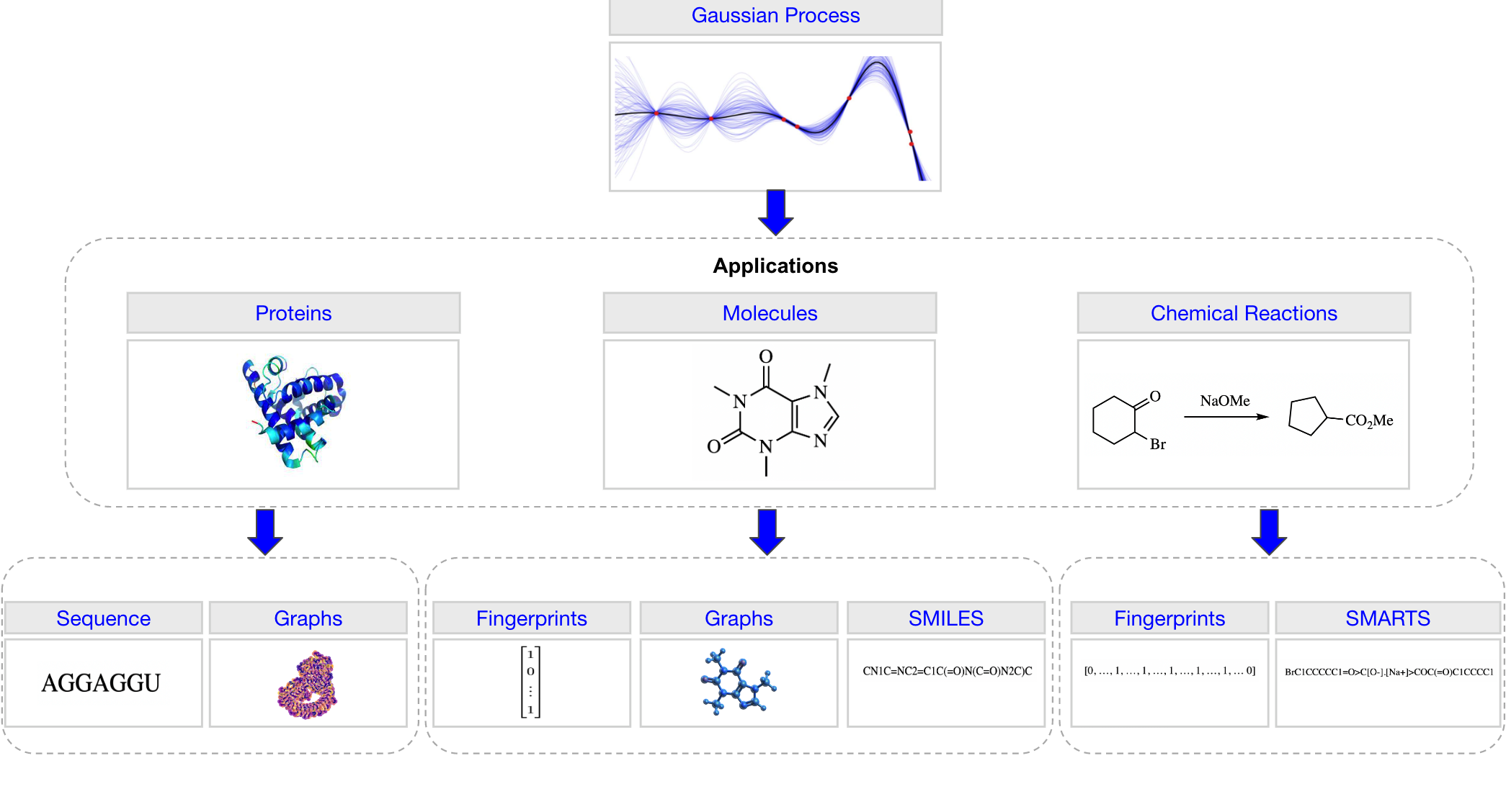
Figure 1: An overview of the applications and representations available in GAUCHE.

2.3 Molecular Representations

We review here the three main categories of molecular representations before describing the kernels that operate on them in section 3. An overview of the representations considered by GAUCHE is provided in Figure 1.

Graphs:

A molecule may be represented as an undirected, labeled graph $\mathcal{G}=(\mathcal{V},\mathcal{E})$ where vertices $\mathcal{V}=\{v_{1},\ldots,v_{N}\}$ represent the atoms of an $N$-atom molecule and edges $\mathcal{E}\subset\mathcal{V}\times\mathcal{V}$ represent covalent bonds between these atoms. Additional information may be incorporated in the form of vertex and edge labels $\mathcal{L}:\mathcal{V}\times\mathcal{E}\to\Sigma_{V}\times\Sigma_{E}$, with common label spaces including attributes such as atom types (e.g. hydrogen, carbon) as vertex labels and bond orders (e.g. single, double) as edge labels.

Fingerprints:

Molecular fingerprints were first introduced for chemical database substructure searching Christie et al. (1993) but were later repurposed for similarity searching Johnson & Maggiora (1990), clustering McGregor & Pallai (1997) and classification Breiman et al. (2017). Extended Connectivity FingerPrints (ECFP) Rogers & Hahn (2010) were introduced as part of the Pipeline project Hassan et al. (2006) with the explicit goal of capturing features relevant for molecular property prediction Xia et al. (2004). ECFP fingerprints operate by assigning initial numeric identifiers to each atom in a molecule. These identifiers are subsequently updated in an iterative fashion based on the identifiers of their neighbours. The number of iterations corresponds to half the diameter of the fingerprint and the naming convention reflects this. For example, ECFP6 fingerprints have a diameter of 6, meaning that 3 iterations of atom identifier reassignment are performed. Each level of iteration appends substructural features of increasing non-locality to an array and the array is then hashed to a bit vector reflecting the presence or absence of those substructures in the molecule.

For property prediction applications a radius of 3 or 4 is recommended. We use a radius of 3 for all experiments in the paper. Additionally we make use of fragment descriptors which are count vectors, each component of which indicates the count of a particular functional group present in a molecule. For example row 1 of the count vector could be an integer representing the number of aliphatic hydroxl groups present in the molecule. We make use of both fingerprint and fragment features computed using RDKit Landrum (2013) as well as the concatenation of the fingerprint and fragment feature vectors, a representation termed fragprints Griffiths et al. (2022) which has shown strong empirical performance. Example representations $\mathbf{x_{f}}$ for fingerprints and $\mathbf{x_{fr}}$ for fragments are given as

$$\mathbf{x_{f}} =\begin{bmatrix}1&0&\cdots&1\end{bmatrix}^{\top},\>\>\>\mathbf{x_{fr}}=\begin{bmatrix}3&0&\cdots&2\end{bmatrix}^{\top}.$$

Strings:

The Simplified Molecular-Input Line-Entry System (SMILES) is a text-based representation of molecules Anderson et al. (1987); Weininger (1988), examples of which are given in Figure 2. Self-Referencing Embedded Strings (SELFIES) Krenn et al. (2020) is an alternative string representation to SMILES such that a bijective mapping exists between a SELFIES string and a molecule.

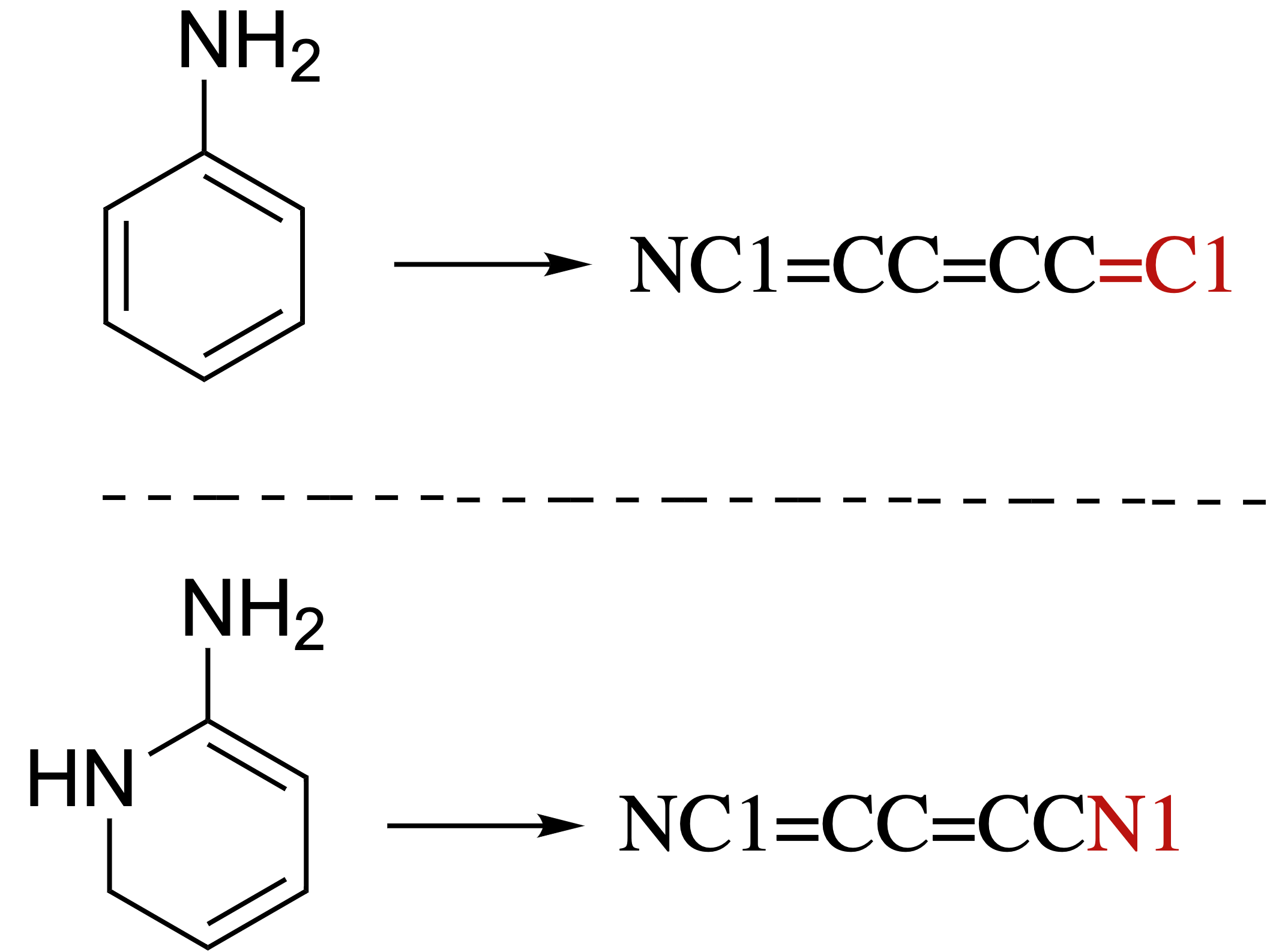
Figure 2: SMILES strings for structurally similar molecules. Similarity is encoded in the string through common contiguous subsequences (black). Local differences are highlighted in red. Molecules chosen for purposes of illustration only.

2.4 Reaction Representations

Chemical reactions consist of (multiple) reactants and reagents that react to form one or more products. The choice of reactant/reagent typically constitutes a categorical design space $\mathcal{X}$. Taking as an example the high-throughput experiments by Ahneman et al. (2018) on Buchwald-Hartwig reactions, the reaction design space consists of 15 aryl and heteroaryl halides, 4 Buchwald ligands, 3 bases, and 23 isoxazole additives.

Concatenated Molecular Representations:

If the number of choices for reactant and reagent is constant, the molecular representations discussed above may be used to encode the selected reactants and reagents, and the vectors for the individual reaction components can be concatenated to build the reaction representation Ahneman et al. (2018); Sandfort et al. (2020). An additional and commonly-used concatenated representation, is the one-hot-encoding (OHE) of the reaction categories where bits specify which of the components in the different reactant and reagent categories is present. In the Buchwald-Hartwig example, the OHE would describe which of the aryl halides, Buchwald ligands, bases and additives are used in the reaction, resulting in a 44-dimensional bit vector Chuang & Keiser (2018).

Differential Reaction Fingerprints:

Inspired by the hand-engineered difference reaction fingerprints by Schneider et al. (2015), Probst et al. (2022) recently introduced the differential reaction fingerprint (DRFP). This reaction fingerprint is constructed by taking the symmetric difference of the sets containing the molecular substructures on both sides of the reaction arrow. Reagents are added to the reactants. The size of the reaction bit vector generated by DRFP is independent of the number of reaction components.

Data-Driven Reaction Fingerprints:

Schwaller et al. (2021a) described data-driven reaction fingerprints using Transformer models such as BERT Kenton et al. (2019) trained in a supervised or an unsupervised fashion on reaction SMILES. Those models can be fine-tuned on the task of interest to learn more specific reaction representations Schwaller et al. (2021b) (RXNFP). Similar to the DRFP, the size of the data-driven reaction fingerprints is independent of the number of reaction components.

2.5 Protein Representations

Proteins are large macromolecules that adopt complex 3D structures. Proteins can be represented in string form describing the underlying amino acid sequence. Graphs at varying degrees of coarseness may be used for structural representations that capture spatial and intramolecular relationships between structural elements, such as atoms, residues, secondary structures and chains. GAUCHE interfaces with Graphein Jamasb et al. (2021), a library for pre-processing and computing graph representations of structural biological data thereby enabling the application of graph kernel-based methods to protein structure.

3 Molecular Kernels

Here we introduce examples of the classes of GAUCHE kernel designed to operate on the molecular representations introduced in section 2.

3.1 Fingerprint Kernels

Scalar Product Kernel:

The simplest kernel to operate on fingerprints is the scalar product or linear kernel defined for vectors $\mathbf{x},\mathbf{x^{\prime}}\in\mathbb{R}^{d}$ as

$$k_{\text{Scalar Product}}(\mathbf{x},\mathbf{x^{\prime}})\coloneqq\sigma_{f}^{2}\cdot\langle\mathbf{x},\mathbf{x^{\prime}}\rangle,$$

where $\sigma_{f}$ is a scalar signal variance hyperparameter and $\langle\cdot,\cdot\rangle$ is the Euclidean inner product.

Tanimoto Kernel:

Introduced as a general similarity metric for binary attributes Gower (1971), the Tanimoto kernel was first used in chemoinformatics in conjunction with non-GP-based kernel methods Ralaivola et al. (2005). It is defined for binary vectors $\mathbf{x},\mathbf{x^{\prime}}\in\{0,1\}^{d}$ for $d\geq 1$ as

$$k_{\text{Tanimoto}}(\mathbf{x},\mathbf{x^{\prime}})\coloneqq\sigma_{f}^{2}\cdot\frac{\langle\mathbf{x},\mathbf{x^{\prime}}\rangle}{\left\lVert\mathbf{x}\right\rVert^{2}+\left\lVert\mathbf{x^{\prime}}\right\rVert^{2}-\langle\mathbf{x},\mathbf{x^{\prime}}\rangle},$$

where $||\cdot||$ is the Euclidean norm.

3.2 String Kernels

String kernels Lodhi et al. (2002); Cancedda et al. (2003) measure the similarity between strings by examining the degree at which their sub-strings differ. In GAUCHE, we implement the SMILES string kernel Cao et al. (2012) which calculates an inner product between the occurrences of sub-strings, considering all contiguous sub-strings made from at most $n$ characters (we set $n=5$ in our experiments). Therefore, for the sub-string count featurisation $\phi:\mathcal{S}\rightarrow\mathbb{R}^{p}$, also known as a bag-of-characters representation Jurafsky & Martin (2000), the SMILES string kernel between two strings $\mathcal{S}$ and $\mathcal{S}^{\prime}$ is given by

$$k_{\textrm{String}}(\mathcal{S},\mathcal{S}^{\prime})\coloneqq\sigma^{2}\cdot\langle\phi(\mathcal{S}),\phi(\mathcal{S}^{\prime})\rangle.$$

More complicated string kernels do exist in the literature, for example GAUCHE also provides an implementation of the subset string kernel Moss et al. (2020a) which allows non-contiguous matches. However, we found that the significant extra computational cost of these methods did not provide improved performance over the more simple SMILES string kernel in the context of molecular data. Note that although named the SMILES string kernel, this kernel can also be applied to any other string representation of molecules e.g. SELFIES.

3.3 Graph Kernels

Graph Kernels:

Graph kernel methods $\phi_{\lambda}:\mathcal{G}\to\mathcal{H}$ map elements from a graph domain $\mathcal{G}$ to a reproducing kernel Hilbert space (RKHS) $\mathcal{H}$, in which an inner product between a pair of graphs $g,g^{\prime}\in\mathcal{G}$ is derived as a measure of similarity

$$k_{\text{Graph}}(g,g^{\prime})\coloneqq\sigma^{2}\cdot\langle\phi_{\lambda}(g),\phi_{\lambda}(g^{\prime})\rangle_{\mathcal{H}},$$

where $\lambda$ denotes kernel-specific hyperarameters and $\sigma^{2}$ is a scale factor. Depending on how $\phi_{\lambda}$ is defined Nikolentzos et al. (2021), the kernel considers different substructural motifs and is characterised by different hyperparameters. Feature functions $\phi_{\lambda}$ from standard libraries also enable maintainable software development, as preprocessing graphs by transforming them into real-valued inputs and utilizing a linear kernel (available in most GP packages) is equivalent to the calculation above.

Frequently-employed approaches include the random walk kernel Vishwanathan et al. (2010), given by a geometric series over the count of matching random walks of increasing length with coefficient $\lambda$, and Weisfeiler-Lehman kernel Shervashidze et al. (2011), given by the inner products of label count vectors over $\lambda$ iterations of the Weisfeiler-Lehman algorithm.

Graph Embedding:

Pretrained graph neural networks (GNNs) Hu et al. (2019); Tom et al. (2022) may also be used to embed molecular graphs in a vector space, which are reminiscent of deep kernel feature functions. Since the GNN is trained on a large amount of data, the representation it produces has the potential to be a more expressive method to encode a molecule (Note: this assumes access to a large pool of in-domain data). Given a vector representation from a pretrained GNN model, we may apply any GP kernel for continuous input spaces, such as the RBF kernel.

4 Experiments

We evaluate GAUCHE on regression, uncertainty quantification (UQ) and BO. The principle goal in conducting regression and UQ benchmarks is to gauge whether performance on these tasks may be used as a proxy for BO performance. BO is a powerful tool for automated scientific discovery but one would prefer to avoid model misspecification in the surrogate when deploying a scheme in the real world. We make use of the following datasets, whose labels are experimentally-determined:

• The Photoswitch Dataset: (Griffiths et al., 2022): The labels, $y$ are the values of the E isomer $\pi-\pi^{*}$ transition wavelength for 392 photoswitch molecules.

• ESOL: (Delaney, 2004): The labels $y$ are the logarithmic aqueous solubility values for 1128 organic small molecules.

• FreeSolv: (Mobley & Guthrie, 2014): The labels $y$ are the hydration free energies for 642 molecules.

• Lipophilicity: The labels $y$ are the octanol/water distribution coefficient (log D at pH 7.4) of 4200 compounds curated from the ChEMBL database Gaulton et al. (2012); Bento et al. (2014).

• Buchwald-Hartwig reactions: (Ahneman et al., 2018) The labels $y$ are the yields for 3955 Pd-catalysed Buchwald–Hartwig C–N cross-couplings.

• Suzuki-Miyaura reactions: (Perera et al., 2018) The labels $y$ are the yields for 5760 Pd-catalysed Suzuki-Miyaura C-C cross-couplings.

4.1 Regression

The regression results for molecular property prediction are reported in Table  1 and for reaction yield prediction in Table B1 of Appendix B. The datasets are split in a train/test ratio of 80/20 (note that validation sets are not required for the GP models since hyperparameters are chosen using the marginal likelihood objective on the train set). Errorbars represent the standard error across 20 random initialisations. All GP models are trained using the L-BFGS-B optimiser Liu & Nocedal (1989). If not mentioned, default settings in the GPyTorch and BoTorch libraries apply. For the SELFIES representation, some molecules could not be featurised and corresponding entries are left blank. The results of Table B1 indicate that the best choice of representation (and hence the choice of kernel) is task-dependent.

For comparison, the regression experiments are repeated for Bayesian neural networks (BNNs), and deep ensembles. The prediction and calibration results are shown in Tables 3 and 4, respectively. The BNNs are based on variational inference (VI) of the posterior distribution of the network weights Blundell et al. (2015), as implemented in Bayesian-Torch Krishnan et al. (2022). The results are shown for a fully connected (FC)-BNN and a GNN with a final Bayesian layer Hwang et al. (2020). The deep ensemble and deep kernel GP both use 1D CNN architectures (Stanton et al., 2022). Further details on the deep probabilistic models are given in Appendix D.

Table 1: Molecular property prediction benchmark. RMSE values for 80/20 train/test split across 20 random trials.

GP Model		Dataset
Kernel	Representation	Photoswitch	ESOL	FreeSolv	Lipophilicity
Tanimoto	fragprints	${\bf 20.9}\pm{\bf 0.7}$	$0.71\pm 0.01$	$1.31\pm 0.06$	$\textbf{0.67}\pm\textbf{0.01}$
	fingerprints	$23.4\pm 0.8$	$1.01\pm 0.01$	$1.93\pm 0.09$	$0.76\pm 0.01$
	fragments	$26.3\pm 0.8$	$0.91\pm 0.01$	$1.49\pm 0.05$	$0.80\pm 0.01$
Scalar Product	fragprints	$22.5\pm 0.7$	$0.88\pm 0.01$	$\textbf{1.27}\pm\textbf{0.02}$	$0.77\pm 0.01$
	fingerprints	$24.8\pm 0.8$	$1.17\pm 0.01$	$1.93\pm 0.07$	$0.84\pm 0.01$
	fragments	$36.6\pm 1.0$	$1.15\pm 0.01$	$1.63\pm 0.03$	$0.97.\pm 0.01$
String	SELFIES	$24.9\pm 0.6$	-	-	-
	SMILES	$24.8\pm 0.7$	$\textbf{0.66}\pm\textbf{0.01}$	$1.31\pm 0.01$	$\textbf{0.68}\pm\textbf{0.01}$
WL Kernel (GraKel)	graph	$22.4\pm 1.4$	$1.04\pm 0.02$	$1.47\pm 0.06$	$0.74\pm 0.05$

4.2 Uncertainty Quantification (UQ)

To quantify the quality of the uncertainty estimates we use three metrics, the negative log predictive density (NLPD), the mean standardised log loss (MSLL) and the quantile coverage error (QCE). We provide the NLPD results in Table 2 and defer the MSLL and QCE results to Appendix C. One trend to note is that uncertainty estimate quality is roughly correlated with regression performance.

Table 2: UQ benchmark. NLPD values for 80/20 train/test split across 20 random trials.

GP Model		Dataset
Kernel	Representation	Photoswitch	ESOL	FreeSolv	Lipophilicity
Tanimoto	fragprints	$\textbf{0.22}\pm\textbf{0.03}$	$0.33\pm 0.01$	$0.28\pm 0.02$	$\textbf{0.71}\pm\textbf{0.01}$
	fingerprints	$0.33\pm 0.03$	$0.71\pm 0.01$	$0.58\pm 0.03$	$0.85\pm 0.01$
	fragments	$0.50\pm 0.04$	$0.57\pm 0.01$	$0.44\pm 0.03$	$0.94\pm 0.02$
Scalar Product	fragprints	$\textbf{0.23}\pm\textbf{0.03}$	$0.53\pm 0.01$	$0.25\pm 0.02$	$0.92\pm 0.01$
	fingerprints	$0.33\pm 0.03$	$0.84\pm 0.01$	$0.64\pm 0.03$	$1.03\pm 0.01$
	fragments	$0.80\pm 0.03$	$0.82\pm 0.01$	$0.54\pm 0.02$	$0.88\pm 0.10$
String	SELFIES	$0.37\pm 0.04$	-	-	-
	SMILES	$0.30\pm 0.04$	$\textbf{0.29}\pm\textbf{0.03}$	$\textbf{0.16}\pm\textbf{0.02}$	$\textbf{0.72}\pm\textbf{0.01}$
WL Kernel (GraKel)	graph	$0.39\pm 0.11$	$0.76\pm 0.001$	$0.47\pm 0.02$	-

Table 3: Molecular property prediction regression benchmark for deep Bayesian models. RMSE of predictions for Bayesian Neural Networks (BNN) and Bayesian Graph Neural Networks (GNN) for 80/20 train/test split across 20 random trials.

Deep Probabilistic Models		Dataset
Model	Representation	Photoswitch	ESOL	FreeSolv	Lipophilicity
FC-BNN	fragprints	$\textbf{20.9}\pm\textbf{0.6}$	$0.88\pm 0.01$	$1.39\pm 0.03$	$0.75\pm 0.01$
	fingerprints	$22.4\pm 0.7$	$1.08\pm 0.02$	$1.93\pm 0.07$	$0.81\pm 0.01$
	fragments	$25.8\pm 0.7$	$1.03\pm 0.01$	$1.48\pm 0.02$	$0.87\pm 0.01$
GNN-BNN	graph	$28.5\pm 1.2$	$0.88\pm 0.01$	$\textbf{0.96}\pm\textbf{0.01}$	$\textbf{0.73}\pm\textbf{0.02}$
CNN Ensemble	SELFIES	$26.4\pm 1.0$	$\textbf{0.67}\pm\textbf{0.01}$	$1.29\pm 0.04$	$\textbf{0.75}\pm\textbf{0.01}$
CNN DKL GP	SELFIES	$25.1\pm 0.8$	$0.94\pm 0.04$	$1.41\pm 0.11$	$0.91\pm 0.01$

Table 4: UQ benchmark. NLPD values of predictions for Bayesian Neural Networks (BNN) and Bayesian Graph Neural Networks (GNN) for 80/20 train/test split across 20 random trials.

Deep Probabilistic Models		Dataset
Model	Representation	Photoswitch	ESOL	FreeSolv	Lipophilicity
FC-BNN	fragprints	$1.63\pm 0.44$	$1.70\pm 0.11$	$1.41\pm 0.38$	$3.82\pm 0.12$
	fingerprints	$2.22\pm 0.56$	$2.59\pm 0.40$	$2.65\pm 0.72$	$3.74\pm 0.10$
	fragments	$0.69\pm 0.09$	$1.93\pm 0.28$	$0.89\pm 0.12$	$5.52\pm 0.23$
GNN-BNN	graph	$1.00\pm 0.13$	$1.70\pm 0.11$	$1.01\pm 0.02$	$\textbf{1.14}\pm\textbf{0.01}$
CNN Ensemble	SELFIES	$4.34\pm 0.55$	$2.91\pm 0.14$	$2.24\pm 0.21$	$2.60\pm 0.06$
CNN DKL GP	SELFIES	$\textbf{0.48}\pm\textbf{0.05}$	$\textbf{0.90}\pm\textbf{0.15}$	$\textbf{0.33}\pm\textbf{0.04}$	$1.46\pm 0.03$

4.3 Bayesian Optimisation

We take forward two of the best-performing kernels, the Tanimoto-fragprint kernel and the SMILES string kernel to undertake BO over the photoswitch and ESOL datasets. Random search is used as a baseline. BO is run for 20 iterations of sequential candidate selection (EI acquisition) where candidates are drawn from 95% of the dataset. The models are initialised with 5% of the dataset. In the case of the photoswitch dataset this corresponds to just 19 molecules. The results are provided in Figure 3. In this ultra-low data setting, common to many areas of synthetic chemistry Griffiths et al. (2022) both models outperform random search, highlighting the real-world use-case for such models in supporting human chemists prioritise candidates for synthesis. Furthermore, one may observe that BO performance is tightly coupled to regression and UQ performance. In the case of the photoswitch dataset, the better-performing Tanimoto model on regression and UQ also achieves better BO performance. Additionally, we run BO on the Buchwald-Hartwig dataset using the Tanimoto kernel for the bit-vector representations DRFP and OHE, and the RBF kernel for RXNFP. All three representations perform similarly, and outperform the random search.

(a) Photoswitch

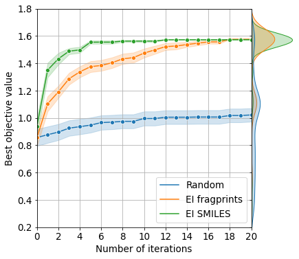
(b) ESOL

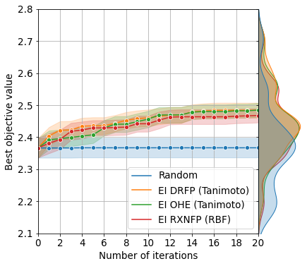
(c) Buchwald-Hartwig reactions

Figure 3: BO performance reporting the standard error from 50 randomly initialised trials (20 for Buchwald-Hartwig). A kernel density estimate over the trials is shown on the right axis. EI fragprints results use the Tanimoto kernel.

5 Related Work

General-purpose GP and BO libraries do not cater for molecular representations. Likewise, general-purpose molecular machine learning libraries do not consider GPs and BO. Here, we review existing libraries, highlighting the niche GAUCHE fills in bridging the GP and molecular machine learning communities.

The closest work to ours is FlowMO Moss & Griffiths (2020), which introduces a basic molecular GP library in the GPflow framework. In this project, we extend the scope of the library to a broader class of molecular representations (graphs), problem settings (BO) and applications (reaction optimisation and protein engineering).

Gaussian Process Libraries:

GP libraries include GPy (Python) GPy (since 2012), GPflow (TensorFlow) Matthews et al. (2017); van der Wilk et al. (2020), GPyTorch (PyTorch) Gardner et al. (2018) and GPJax (Jax) Pinder & Dodd (2022) while examples of recent BO libraries include BoTorch (PyTorch) Balandat et al. (2020), Dragonfly (Python) Kandasamy et al. (2020), HEBO (PyTorch) Cowen-Rivers et al. (2020) and Trieste (Tensorflow) Berkeley et al. (2022). The aforementioned libraries do not explicitly support molecular representations. Extension to cover molecular representations however is nontrivial, requiring implementations of bespoke GP kernels for bit vector, string and graph inputs together with modifications to BO schemes to consider acquisition function evaluations over a discrete set of heldout molecules, a setting commonly encountered in virtual screening Pyzer-Knapp (2020); Graff et al. (2022).

Molecular Machine Learning Libraries:

Molecular machine learning libraries include DeepChem Ramsundar et al. (2019), DGL-LifeSci Li et al. (2021) and TorchDrug Zhu et al. (2022). DeepChem features a broad range of model implementations and tasks, while DGL-LifeSci focuses on graph neural networks. TorchDrug caters for applications including property prediction, representation learning, retrosynthesis, biomedical knowledge graph reasoning and molecule generation.

GP implementations are not included, however, in the aforementioned libraries. In terms of atomistic systems, DScribe Himanen et al. (2020) features, amongst other methods, the Smooth Overlap of Atomic Positions (SOAP) representation Bartók et al. (2013) which is typically used in conjunction with a GP model to learn atomistic properties. Automatic Selection And Prediction (ASAP) Cheng et al. (2020) also principally focusses on atomistic properties as well as dimensionality reduction and visualisation techniques for materials and molecules. Lastly, the Graphein library focusses on graph representations of proteins Jamasb et al. (2021).

Graph Kernel Libraries:

Graph kernel libraries include GraKel Siglidis et al. (2020), graphkit-learn Jia et al. (2021), graphkernels Sugiyama et al. (2018), graph-kernels Sugiyama & Borgwardt (2015), pykernels (https://github.com/gmum/pykernels) and ChemoKernel Gaüzére et al. (2012). The aforementioned libraries focus on CPU implementations in Python. Extending graph kernel computation to GPUs has been noted as an important direction for future research Ghosh et al. (2018). In our work, we build on the GraKel library by interfacing it with GPyTorch, facilitating GP regression with GPU computation. Furthermore, we enable the graph kernel hyperparameters to be learned through the marginal likelihood objective as opposed to being pre-specified and fixed upfront. It is worth noting that GAUCHE extends the applicability of GPU-enabled GPs to general graph-structured inputs beyond just molecules and proteins.

Molecular Bayesian Optimisation:

BO over molecular space can be divided into two classes. In the first class, molecules are encoded into the latent space of a variational autoencoder (VAE) Gómez-Bombarelli et al. (2018). BO is then performed over the continuous latent space and queried molecules are decoded back to the original space. Much work on VAE-BO has focussed on improving the synergy between the surrogate model and the VAE Griffiths et al. (2021b); Griffiths & Hernández-Lobato (2020); Tripp et al. (2020); Deshwal & Doppa (2021); Grosnit et al. (2021); Verma & Chakraborty (2021); Maus et al. (2022); Stanton et al. (2022). One of the defining characteristics of VAE-BO is that it enables the generation of new molecular structures.

In the second class of methods, BO is performed directly over the original discrete space of molecules. In this setting it is not possible to generate new structures and so a candidate set of queryable molecules is defined. The inability to generate new structures however, is not a bottleneck to molecule discovery as the principle concern is how best to explore existing candidate sets. These candidate sets are also known as molecular libraries in the virtual screening literature Pyzer-Knapp et al. (2015).

To date, there has been little work on BO directly over discrete molecular spaces. In Moss et al. (2020a), the authors use a string kernel GP trained on SMILES to perform BO to select from a candidate set of molecules. In Korovina et al. (2020), an optimal transport kernel GP is used for BO over molecular graphs. In Häse et al. (2021a) a surrogate based on the Nadarya-Watson estimator is defined such that the kernel density estimates are inferred using BNNs. The model is then trained on molecular descriptors. Lastly, in Hernández-Lobato et al. (2017) and Vakili et al. (2021) a BNN and a sparse GP respectively are trained on fingerprint representations of molecules. In the case of the sparse GP the authors select an ArcCosine kernel. It is a longstanding aim of the GAUCHE Project to compare the efficacy of VAE-BO against vanilla BO on real-world molecule discovery tasks.

Chemical Reaction Optimisation:

Chemical reactions describe how reactants transform into products. Reagents (catalysts, solvents, and additives) and reaction conditions heavily impact the outcome of chemical reactions. Typically the objective is to maximise the reaction yield (the amount of product compared to the theoretical maximum) Ahneman et al. (2018), in asymmetric synthesis, where the reactions could result in different enantiomers, to maximise the enantiomeric excess Zahrt et al. (2019), or to minimise the E-factor, which is the ratio between waste materials and the desired product Schweidtmann et al. (2018).

A diverse set of studies have evaluated the optimisation of chemical reactions in single and multi-objective settings Schweidtmann et al. (2018); Müller et al. (2022). Felton et al. (2021) and Häse et al. (2021b) benchmarked reaction optimisation algorithms in low-dimensional settings including reaction conditions, such as time, temperature, and concentrations. Shields et al. (2021) suggested BO as a general tool for chemical reaction optimisation and benchmarked their approach against human experts. Haywood et al. (2021) compared the yield prediction performance of different kernels and Pomberger et al. (2022) the impact of various molecular representations.

In all reaction optimisation studies above, the representations of the different categories of reactants and reagents are concatenated to generate the reaction input vector, which could lead to limitations if another type of reagent is suddenly considered. Moreover, most studies concluded that simple one-hot encodings (OHE) perform at least on par with more elaborate molecular representations in the low-data regime Shields et al. (2021); Pomberger et al. (2022); Hickman et al. (2022). In GAUCHE, we introduce reaction fingerprint kernels, based on existing reaction fingerprints Schwaller et al. (2021a); Probst et al. (2022) and work independently of the number of reactant and reagent categories.

6 Conclusions and Future Work

We have introduced GAUCHE, a library for GAUssian Processes in CHEmistry with the aim of providing tools for uncertainty quantification and Bayesian optimisation that may hopefully be deployed for screening in laboratory settings. Future work is centred along two axes:

1. Methodology: We seek to incorporate more sophisticated GP-based optimisation and active learning loops in chemistry applications Eyke et al. (2020); Rankovic et al. (2022); Griffiths (2023), such as the application of ideas from batch González et al. (2016), multi-task Swersky et al. (2013), multi-fidelity Moss et al. (2020b), multi-objective Knowles (2006), and quantile Torossian et al. (2020) optimisation. We will also investigate the use of approximate Gaussian processes Titsias (2009); Hensman et al. (2013) and their recent adaptations for BO Maddox et al. (2021); Chang et al. (2022); Moss et al. (2022; 2023) to allow our methods to handle larger evaluation budgets.

2. User Feedback: We seek to further grow our userbase and solicit feedback from laboratory practitioners on the most common use-cases for BO and GP modelling in molecular discovery campaigns. Of particular interest is the relative prevalance of molecule generation and optimisation via VAE-BO compared to AL/BO to prioritise molecules in high-throughput screening settings.

1. Introduction 1

2. Background 2

   1. Gaussian Processes 2

      1. Notation

      2. Prediction

      3. Kernels

      4. GP Training

   2. Bayesian Optimisation 2

   3. Molecular Representations 3

      1. Graphs

      2. Fingerprints

      3. Strings

   4. Reaction Representations 3

      1. Concatenated Molecular Representations

      2. Differential Reaction Fingerprints

   5. Protein Representations 4

3. Molecular Kernels 4

   1. Fingerprint Kernels

      1. Scalar Product Kernel

      2. Tanimoto Kernel

   2. String Kernels

   3. Graph Kernels

      1. Graph Kernel

      2. Graph Embedding

4. Experiments 5

   1. Regression

   2. Uncertainty Quantification (UQ)

   3. Bayesian Optimisation

5. Related Work 6

   1. Gaussian Process Libraries

   2. Molecular Machine Learning Libraries

   3. Graph Kernel Libraries

   4. Molecular Bayesian Optimisation

   5. Chemical Reaction Optimisation

6. Conclusions and Future Work 8

1. Coding Kernels in GAUCHE 16

2. Chemical Reaction Yield Prediction Experiments 16

3. Uncertainty Quantification Experiments 16

4. Deep Probabilistic Models 17

Appendix A Coding Kernels in GAUCHE

We provide an example of the class definition for the Tanimoto kernel in GAUCHE below

⬇

class TanimotoGP(ExactGP):

def __init__(self, train_x, train_y, likelihood):

super(TanimotoGP, self).__init__(train_x,

train_y,

likelihood)

self.mean_module = ConstantMean()

# We use the Tanimoto kernel to work with

# molecular fingerprint representations

self.covar_module = ScaleKernel(TanimotoKernel())

def forward(self, x):

mean_x = self.mean_module(x)

covar_x = self.covar_module(x)

return MultivariateNormal(mean_x, covar_x)

and an example definition of a black box kernel (where gradients with respect to hyperparameters and input labels are not required).

⬇

class WLKernel(gauche.Kernel):

def __init__(self):

super().__init__()

self.kernel = grakel.kernels.WeisfeilerLehman()

@lru_cache(maxsize=3)

def kern(self, X):

return tensor(self.kernel.fit_transform(X.data))

class GraphGP(gauche.SIGP):

def __init__(self, train_x, train_y, likelihood):

super().__init__(train_x, train_y, likelihood)

self.mean = ConstantMean()

self.covariance = WLKernel()

def forward(self, X):

# X is a gauche.Inputs instance, with X.data

# holding a list of grakel.Graph instances.

mean = self.mean(zeros(len(X.data), 1))

covariance = self.covariance(X)

return MultivariateNormal(mean, covariance)

Importantly, GAUCHE inherits all the facilities of GPyTorch and GraKel allowing a broad range of of models to be defined on molecular inputs such as deep GPs, multioutput GPs and heteroscedastic GPs.

Appendix B Chemical Reaction Yield Prediction Experiments

Further regression and uncertainty quantification experiments are presented in Table B1. The differential reaction fingerprint in conjunction with the Tanimoto kernel is the best-performing reaction representation.

Table B1: Chemical reaction regression benchmark. 80/20 train/test split across 20 random trials.

GP Model		Buchwald-Hartwig
Kernel	Representation	RMSE $\downarrow$	$R^{2}$ score $\uparrow$	MSLL $\downarrow$	QCE $\downarrow$
Tanimoto	OHE	$7.94\pm 0.05$	$0.91\pm 0.001$	$-0.06\pm 0.002$	$0.011\pm 0.001$
	DRFP	$\textbf{6.48}\pm\textbf{0.45}$	$\textbf{0.94}\pm\textbf{0.015}$	$\textbf{-0.15}\pm\textbf{0.07}$	$0.027\pm 0.002$
Scalar Product	OHE	$15.23\pm 0.052$	$0.69\pm 0.002$	$0.57\pm 0.002$	$0.008\pm 0.001$
	DRFP	$14.63\pm 0.050$	$0.71\pm 0.002$	$0.55\pm 0.002$	$0.010\pm 0.001$
RBF	RXNFP	$10.79\pm 0.049$	$0.84\pm 0.001$	$0.37\pm 0.005$	$0.024\pm 0.001$
		Suzuki-Miyaura
Tanimoto	OHE	$11.18\pm 0.036$	$0.83\pm 0.001$	$0.23\pm 0.001$	$0.007\pm 0.001$
	DRFP	$11.46\pm 0.038$	$0.83\pm 0.001$	$0.25\pm 0.006$	$0.019\pm 0.000$
Scalar Product	OHE	$19.91\pm 0.042$	$0.47\pm 0.003$	$0.82\pm 0.001$	$0.012\pm 0.001$
	DRFP	$19.66\pm 0.042$	$0.52\pm 0.003$	$0.81\pm 0.001$	$0.014\pm 0.001$
RBF	RXNFP	$13.83\pm 0.048$	$0.75\pm 0.002$	$0.50\pm 0.001$	$0.007\pm 0.001$

Appendix C Uncertainty Quantification Experiments

In Table C2 and Table C3 we present further uncertainty quantification metrics. Numerical errors were encountered with the WL kernel on the large lipophilicity dataset which invalidated the results and so the corresponding entry is left blank. The native random walk kernel was discontinued (for the time being) due to poor performance!

Table C2: UQ Benchmark. MSLL Values ($\downarrow$) for 80/20 Train/Test Split.

GP Model		Dataset
Kernel	Representation	Photoswitch	ESOL	FreeSolv	Lipophilicity
Tanimoto	fragprints	$\textbf{0.06}\pm\textbf{0.01}$	$0.17\pm 0.04$	$0.16\pm 0.02$	$\textbf{0.50}\pm\textbf{0.006}$
	fingerprints	$0.16\pm 0.01$	$0.55\pm 0.01$	$0.42\pm 0.02$	$0.63\pm 0.004$
	fragments	$0.27\pm 0.01$	$0.34\pm 0.04$	$0.24\pm 0.02$	$0.72\pm 0.003$
Scalar Product	fragprints	$0.03\pm 0.01$	$0.32\pm 0.004$	$0.06\pm 0.01$	$0.67\pm 0.003$
	fingerprints	$0.11\pm 0.01$	$0.64\pm 0.006$	$0.41\pm 0.02$	$0.79\pm 0.003$
	fragments	$0.56\pm 0.01$	$0.58\pm 0.005$	$0.29\pm 0.01$	$0.94\pm 0.003$
String	SELFIES	$0.13\pm 0.01$	-	-	-
	SMILES	$\textbf{0.08}\pm\textbf{0.02}$	$\textbf{0.03}\pm\textbf{0.005}$	$\textbf{0.03}\pm\textbf{0.02}$	$\textbf{0.52}\pm\textbf{0.002}$
WL Kernel (GraKel)	graph	$0.14\pm 0.03$	$0.54\pm 0.01$	$0.26\pm 0.01$	-

Table C3: UQ benchmark. QCE values ($\downarrow$) for 80/20 train/test split across 20 random trials.

GP Model		Dataset
Kernel	Representation	Photoswitch	ESOL	FreeSolv	Lipophilicity
Tanimoto	fragprints	$\textbf{0.019}\pm\textbf{0.003}$	$0.023\pm 0.002$	$0.023\pm 0.002$	$0.006\pm 0.002$
	fingerprints	$0.023\pm 0.003$	$0.022\pm 0.002$	$0.018\pm 0.003$	$0.006\pm 0.001$
	fragments	$0.025\pm 0.005$	$0.012\pm 0.002$	$0.014\pm 0.002$	$0.009\pm 0.002$
Scalar Product	fragprints	$0.033\pm 0.006$	$0.010\pm 0.002$	$0.017\pm 0.003$	$0.010\pm 0.001$
	fingerprints	$0.036\pm 0.006$	$0.014\pm 0.002$	$0.016\pm 0.002$	$0.009\pm 0.001$
	fragments	$0.027\pm 0.004$	$0.012\pm 0.003$	$0.021\pm 0.003$	$0.010\pm 0.001$
String	SELFIES	$0.031\pm 0.006$	-	-	-
	SMILES	$0.024\pm 0.003$	$0.016\pm 0.002$	$0.019\pm 0.003$	$0.005\pm 0.001$
WL Kernel (GraKel)	graph	$0.025\pm 0.007$	$0.011\pm 0.004$	$0.019\pm 0.009$	$0.066\pm 0.014$

Appendix D Deep Probabilistic Models

There is a growing body of work applying deep learning to molecular property prediction (Walters & Barzilay, 2020). Therefore in addition to evaluating GPs with varying shallow kernel functions, we repeat the regression experiments with a range of deep Bayesian models, varying both the network architecture and the Bayesian inference procedure. We evaluate the following models:

• FC-BNN + VI is a fully connected neural network with a single variational inference (VI) Bayesian layer with 100 nodes, followed by the rectified linear unit (ReLU) activation, and a final output layer. Trained with early stopping.

• GNN-BNN + VI utilises the same network and graph features as used for the graph embeddings Hu et al. (2019) followed by a final VI Bayesian layer. Trained with early stopping.

• CNN DKL GP is the same approach and architecture used by Stanton et al. (2022) to predict molecular properties for Bayesian optimisation. Using SELFIES representations, a 1D CNN encoder is shared and trained jointly through a generative masked language model (MLM) head (Kenton et al., 2019) and a discriminative deep kernel GP head (Wilson et al., 2016).

• CNN Ensemble is a deep ensemble of 1D CNN networks, also implemented by Stanton et al. (2022), where each ensemble component uses the SELFIES molecule representation and is trained independently to minimize the MSE loss. Deep ensembles have been shown to provide high-fidelity approximations of Bayesian model averages relative to alternative approaches such as Laplace approximation or VI (Izmailov et al., 2021).

To summarize our results in Tables 3 & 4, we find that deep Bayesian models generally do not outperform discrete string kernels or shallow continuous kernels on hand-crafted features (e.g. fragprints) on the datasets we consider, although in some cases performance is very competitive. Our results suggest that for small to mid-sized molecular datasets the Tanimoto kernel combined with fragprint representations in particular is a very compelling option, with good accuracy, calibration, and runtime across all tasks.

References

- Ahneman et al. (2018) Ahneman, D. T., Estrada, J. G., Lin, S., Dreher, S. D., and Doyle, A. G. Predicting reaction performance in C–N cross-coupling using machine learning. Science, 2018.
- Anderson et al. (1987) Anderson, E., Veith, G. D., and Weininger, D. SMILES, a line notation and computerized interpreter for chemical structures. Environmental Research Laboratory, 1987.
- Balandat et al. (2020) Balandat, M., Karrer, B., Jiang, D., Daulton, S., Letham, B., Wilson, A. G., and Bakshy, E. BoTorch: A framework for efficient Monte-Carlo Bayesian optimization. Advances in Neural Information Processing Systems, 2020.
- Bartók et al. (2013) Bartók, A. P., Kondor, R., and Csányi, G. On representing chemical environments. Physical Review B, 2013.
- Bengio (2011) Bengio, Y. What are some Advantages of Using Gaussian Process Models vs Neural Networks?, 2011. https://www.quora.com/What-are-some-advantages-of-using-Gaussian-Process-Models-vs-Neural-Networks.
- Bento et al. (2014) Bento, A. P., Gaulton, A., Hersey, A., Bellis, L. J., Chambers, J., Davies, M., Krüger, F. A., Light, Y., Mak, L., McGlinchey, S., et al. The ChEMBL bioactivity database: An update. Nucleic Acids Research, 2014.
- Berkeley et al. (2022) Berkeley, J., Moss, H. B., Artemev, A., Pascual-Diaz, S., Granta, U., Stojic, H., Couckuyt, I., Qing, J., Loka, N., Paleyes, A., Ober, S. W., and Picheny, V. Trieste. https://github.com/secondmind-labs/trieste, 2022.
- Blundell et al. (2015) Blundell, C., Cornebise, J., Kavukcuoglu, K., and Wierstra, D. Weight uncertainty in neural network. In International conference on machine learning, pp. 1613–1622. PMLR, 2015.
- Breiman et al. (2017) Breiman, L., Friedman, J. H., Olshen, R. A., and Stone, C. J. Classification and regression trees. Routledge, 2017.
- Brochu et al. (2010) Brochu, E., Cora, V. M., and De Freitas, N. A tutorial on Bayesian optimization of expensive cost functions, with application to active user modeling and hierarchical reinforcement learning. arXiv preprint arXiv:1012.2599, 2010.
- Cancedda et al. (2003) Cancedda, N., Gaussier, E., Goutte, C., and Renders, J. M. Word sequence kernels. Journal of Machine Learning Research, 2003.
- Cao et al. (2012) Cao, D.-S., Zhao, J.-C., Yang, Y.-N., Zhao, C.-X., Yan, J., Liu, S., Hu, Q.-N., Xu, Q.-S., and Liang, Y.-Z. In silico toxicity prediction by support vector machine and SMILES representation-based string kernel. SAR and QSAR in Environmental Research, 2012.
- Capecchi et al. (2020) Capecchi, A., Probst, D., and Reymond, J.-L. One molecular fingerprint to rule them all: Drugs, biomolecules, and the metabolome. Journal of Cheminformatics, 2020.
- Chang et al. (2022) Chang, P. E., Verma, P., John, S., Picheny, V., Moss, H., and Solin, A. Fantasizing with dual gps in bayesian optimization and active learning. arXiv preprint arXiv:2211.01053, 2022.
- Cheng et al. (2020) Cheng, B., Griffiths, R.-R., Wengert, S., Kunkel, C., Stenczel, T., Zhu, B., Deringer, V. L., Bernstein, N., Margraf, J. T., Reuter, K., et al. Mapping materials and molecules. Accounts of Chemical Research, 2020.
- Christie et al. (1993) Christie, B. D., Leland, B. A., and Nourse, J. G. Structure searching in chemical databases by direct lookup methods. Journal of Chemical Information and Computer Sciences, 1993.
- Chuang & Keiser (2018) Chuang, K. V. and Keiser, M. J. Comment on “predicting reaction performance in c–n cross-coupling using machine learning”. Science, 2018.
- Cowen-Rivers et al. (2020) Cowen-Rivers, A. I., Lyu, W., Tutunov, R., Wang, Z., Grosnit, A., Griffiths, R. R., Maraval, A. M., Jianye, H., Wang, J., Peters, J., et al. An empirical study of assumptions in Bayesian optimisation. arXiv preprint arXiv:2012.03826, 2020.
- Delaney (2004) Delaney, J. S. ESOL: Estimating aqueous solubility directly from molecular structure. Journal of Chemical Information and Computer Sciences, 2004.
- Deshwal & Doppa (2021) Deshwal, A. and Doppa, J. Combining latent space and structured kernels for Bayesian optimization over combinatorial spaces. Advances in Neural Information Processing Systems, 2021.
- Du et al. (2022) Du, Y., Fu, T., Sun, J., and Liu, S. Molgensurvey: A systematic survey in machine learning models for molecule design. arXiv preprint arXiv:2203.14500, 2022.
- Duvenaud et al. (2015) Duvenaud, D. K., Maclaurin, D., Iparraguirre, J., Bombarell, R., Hirzel, T., Aspuru-Guzik, A., and Adams, R. P. Convolutional networks on graphs for learning molecular fingerprints. Advances in Neural Information Processing Systems, 2015.
- Eyke et al. (2020) Eyke, N. S., Green, W. H., and Jensen, K. F. Iterative experimental design based on active machine learning reduces the experimental burden associated with reaction screening. Reaction Chemistry & Engineering, 2020.
- Felton et al. (2021) Felton, K. C., Rittig, J. G., and Lapkin, A. A. Summit: Benchmarking machine learning methods for reaction optimisation. Chemistry-Methods, 2021.
- Frazier (2018) Frazier, P. I. A tutorial on Bayesian optimization. arXiv preprint arXiv:1807.02811, 2018.
- Gardner et al. (2018) Gardner, J., Pleiss, G., Weinberger, K. Q., Bindel, D., and Wilson, A. G. GPyTorch: Blackbox matrix-matrix Gaussian process inference with GPU acceleration. In Advances in Neural Information Processing Systems, 2018.
- Gaulton et al. (2012) Gaulton, A., Bellis, L. J., Bento, A. P., Chambers, J., Davies, M., Hersey, A., Light, Y., McGlinchey, S., Michalovich, D., Al-Lazikani, B., et al. ChEMBL: A large-scale bioactivity database for drug discovery. Nucleic Acids Research, 2012.
- Gaüzére et al. (2012) Gaüzére, B., Brun, L., Villemin, D., and Brun, M. Graph kernels based on relevant patterns and cycle information for chemoinformatics. In Proceedings of the 21st International Conference on Pattern Recognition, 2012.
- Ghosh et al. (2018) Ghosh, S., Das, N., Gonçalves, T., Quaresma, P., and Kundu, M. The journey of graph kernels through two decades. Computer Science Review, 2018.
- Gómez-Bombarelli et al. (2018) Gómez-Bombarelli, R., Wei, J. N., Duvenaud, D., Hernández-Lobato, J. M., Sánchez-Lengeling, B., Sheberla, D., Aguilera-Iparraguirre, J., Hirzel, T. D., Adams, R. P., and Aspuru-Guzik, A. Automatic chemical design using a data-driven continuous representation of molecules. ACS Central Science, 2018.
- González et al. (2016) González, J., Dai, Z., Hennig, P., and Lawrence, N. Batch Bayesian optimization via local penalization. In Artificial Intelligence and Statistics, 2016.
- Gower (1971) Gower, J. C. A general coefficient of similarity and some of its properties. Biometrics, 1971.
- GPy (since 2012) GPy. GPy: A Gaussian process framework in Python. http://github.com/SheffieldML/GPy, since 2012.
- Graff et al. (2022) Graff, D. E., Aldeghi, M., Morrone, J. A., Jordan, K. E., Pyzer-Knapp, E. O., and Coley, C. W. Self-focusing virtual screening with active design space pruning. arXiv preprint arXiv:2205.01753, 2022.
- Griffiths (2023) Griffiths, R.-R. Gaussian Processes at Extreme Lengthscales: From Molecules to Black Holes. PhD thesis, University of Cambridge, 2023.
- Griffiths & Hernández-Lobato (2020) Griffiths, R.-R. and Hernández-Lobato, J. M. Constrained Bayesian optimization for automatic chemical design using variational autoencoders. Chemical Science, 2020.
- Griffiths et al. (2021a) Griffiths, R.-R., Jiang, J., Buisson, D. J., Wilkins, D., Gallo, L. C., Ingram, A., Grupe, D., Kara, E., Parker, M. L., Alston, W., et al. Modeling the multiwavelength variability of Mrk 335 using Gaussian processes. The Astrophysical Journal, 914(2):144, 2021a.
- Griffiths et al. (2021b) Griffiths, R.-R., Schwaller, P., and Lee, A. A. Dataset bias in the natural sciences: A case study in chemical reaction prediction and synthesis design. arXiv preprint arXiv:2105.02637, 2021b.
- Griffiths et al. (2022) Griffiths, R.-R., Greenfield, J. L., Thawani, A. R., Jamasb, A. R., Moss, H. B., Bourached, A., Jones, P., McCorkindale, W., Aldrick, A. A., Fuchter, M. J., et al. Data-driven discovery of molecular photoswitches with multioutput Gaussian processes. Chemical Science, 2022.
- Grosnit et al. (2020) Grosnit, A., Cowen-Rivers, A. I., Tutunov, R., Griffiths, R.-R., Wang, J., and Bou-Ammar, H. Are we forgetting about compositional optimisers in Bayesian optimisation? arXiv preprint arXiv:2012.08240, 2020.
- Grosnit et al. (2021) Grosnit, A., Tutunov, R., Maraval, A. M., Griffiths, R.-R., Cowen-Rivers, A. I., Yang, L., Zhu, L., Lyu, W., Chen, Z., Wang, J., et al. High-dimensional Bayesian optimisation with variational autoencoders and deep metric learning. arXiv preprint arXiv:2106.03609, 2021.
- Häse et al. (2021a) Häse, F., Aldeghi, M., Hickman, R. J., Roch, L. M., and Aspuru-Guzik, A. Gryffin: An algorithm for Bayesian optimization of categorical variables informed by expert knowledge. Applied Physics Reviews, 2021a.
- Häse et al. (2021b) Häse, F., Aldeghi, M., Hickman, R. J., Roch, L. M., Christensen, M., Liles, E., Hein, J. E., and Aspuru-Guzik, A. Olympus: A benchmarking framework for noisy optimization and experiment planning. Machine Learning: Science and Technology, 2021b.
- Hassan et al. (2006) Hassan, M., Brown, R. D., Varma-O’Brien, S., and Rogers, D. Cheminformatics analysis and learning in a data pipelining environment. Molecular Diversity, 2006.
- Haywood et al. (2021) Haywood, A. L., Redshaw, J., Hanson-Heine, M. W., Taylor, A., Brown, A., Mason, A. M., Gärtner, T., and Hirst, J. D. Kernel methods for predicting yields of chemical reactions. Journal of Chemical Information and Modeling, 2021.
- Hennig & Schuler (2012) Hennig, P. and Schuler, C. J. Entropy search for information-efficient global optimization. Journal of Machine Learning Research, 2012.
- Hensman et al. (2013) Hensman, J., Fusi, N., and Lawrence, N. D. Gaussian processes for big data. arXiv preprint arXiv:1309.6835, 2013.
- Hernández-Lobato et al. (2014) Hernández-Lobato, J. M., Hoffman, M. W., and Ghahramani, Z. Predictive entropy search for efficient global optimization of black-box functions. Advances in Neural Information Processing Systems, 2014.
- Hernández-Lobato et al. (2017) Hernández-Lobato, J. M., Requeima, J., Pyzer-Knapp, E. O., and Aspuru-Guzik, A. Parallel and distributed Thompson sampling for large-scale accelerated exploration of chemical space. In International Conference on Machine Learning, 2017.
- Hickman et al. (2022) Hickman, R., Ruža, J., Roch, L., Tribukait, H., and García-Durán, A. Equipping data-driven experiment planning for self-driving laboratories with semantic memory: Case studies of transfer learning in chemical reaction optimization. ChemRxiv, 2022.
- Himanen et al. (2020) Himanen, L., Jäger, M. O., Morooka, E. V., Canova, F. F., Ranawat, Y. S., Gao, D. Z., Rinke, P., and Foster, A. S. DScribe: Library of descriptors for machine learning in materials science. Computer Physics Communications, 2020.
- Hu et al. (2019) Hu, W., Liu, B., Gomes, J., Zitnik, M., Liang, P., Pande, V., and Leskovec, J. Strategies for pre-training graph neural networks. In International Conference on Learning Representations, 2019.
- Hwang et al. (2020) Hwang, D., Lee, G., Jo, H., Yoon, S., and Ryu, S. A benchmark study on reliable molecular supervised learning via Bayesian learning. arXiv preprint arXiv:2006.07021, 2020.
- Izmailov et al. (2021) Izmailov, P., Vikram, S., Hoffman, M. D., and Wilson, A. G. G. What are bayesian neural network posteriors really like? In International conference on machine learning, pp. 4629–4640. PMLR, 2021.
- Jablonka et al. (2021) Jablonka, K. M., Jothiappan, G. M., Wang, S., Smit, B., and Yoo, B. Bias free multiobjective active learning for materials design and discovery. Nature Communications, 2021.
- Jamasb et al. (2021) Jamasb, A. R., Viñas, R., Ma, E. J., Harris, C., Huang, K., Hall, D., Lió, P., and Blundell, T. L. Graphein - a Python library for geometric deep learning and network analysis on protein structures and interaction networks. bioRxiv, 2021.
- Jia et al. (2021) Jia, L., Gaüzère, B., and Honeine, P. graphkit-learn: A Python library for graph kernels based on linear patterns. Pattern Recognition Letters, 2021.
- Johnson & Maggiora (1990) Johnson, M. A. and Maggiora, G. M. Concepts and applications of molecular similarity. Wiley, 1990.
- Jones et al. (1998) Jones, D. R., Schonlau, M., and Welch, W. J. Efficient global optimization of expensive black-box functions. Journal of Global Optimization, 1998.
- Jurafsky & Martin (2000) Jurafsky, D. and Martin, J. H. An introduction to natural language processing, computational linguistics, and speech recognition, 2000.
- Kandasamy et al. (2020) Kandasamy, K., Vysyaraju, K. R., Neiswanger, W., Paria, B., Collins, C. R., Schneider, J., Poczos, B., and Xing, E. P. Tuning hyperparameters without grad students: Scalable and robust Bayesian optimisation with Dragonfly. Journal of Machine Learning Research, 2020.
- Kearnes et al. (2016) Kearnes, S., McCloskey, K., Berndl, M., Pande, V., and Riley, P. Molecular graph convolutions: Moving beyond fingerprints. Journal of Computer-Aided Molecular Design, 2016.
- Kenton et al. (2019) Kenton, J. D., Ming-Wei, C., and Toutanova, L. K. Bert: Pre-training of deep bidirectional transformers for language understanding. In Proceedings of NAACL-HLT, pp. 4171–4186, 2019.
- Knowles (2006) Knowles, J. Parego: A hybrid algorithm with on-line landscape approximation for expensive multiobjective optimization problems. IEEE Transactions on Evolutionary Computation, 10(1):50–66, 2006.
- Korovina et al. (2020) Korovina, K., Xu, S., Kandasamy, K., Neiswanger, W., Poczos, B., Schneider, J., and Xing, E. ChemBO: Bayesian optimization of small organic molecules with synthesizable recommendations. In International Conference on Artificial Intelligence and Statistics, 2020.
- Krenn et al. (2020) Krenn, M., Häse, F., Nigam, A., Friederich, P., and Aspuru-Guzik, A. Self-referencing embedded strings (SELFIES): A 100% robust molecular string representation. Machine Learning: Science and Technology, 2020.
- Krishnan et al. (2022) Krishnan, R., Esposito, P., and Subedar, M. Bayesian-torch: Bayesian neural network layers for uncertainty estimation. https://github.com/IntelLabs/bayesian-torch, January 2022. URL https://doi.org/10.5281/zenodo.5908307.
- Kushner (1963) Kushner, H. J. A new method of locating the maximum point of an arbitrary multipeak curve in the presence of noise. In Joint Automatic Control Conference, 1963.
- Landrum (2013) Landrum, G. RDKit: A software suite for cheminformatics, computational chemistry, and predictive modeling, 2013.
- Li et al. (2021) Li, M., Zhou, J., Hu, J., Fan, W., Zhang, Y., Gu, Y., and Karypis, G. DGL-LifeSci: An open-source toolkit for deep learning on graphs in life science. ACS Omega, 2021.
- Liu & Nocedal (1989) Liu, D. C. and Nocedal, J. On the limited memory BFGS method for large scale optimization. Mathematical Programming, 1989.
- Lodhi et al. (2002) Lodhi, H., Saunders, C., Shawe-Taylor, J., Cristianini, N., and Watkins, C. Text classification using string kernels. Journal of Machine Learning Research, 2002.
- MacKay et al. (2003) MacKay, D. J., Mac Kay, D. J., et al. Information theory, inference and learning algorithms. Cambridge University Press, 2003.
- Maddox et al. (2021) Maddox, W. J., Stanton, S., and Wilson, A. G. Conditioning sparse variational gaussian processes for online decision-making. Advances in Neural Information Processing Systems, 34:6365–6379, 2021.
- Matthews et al. (2017) Matthews, A. G., van der Wilk, M., Nickson, T., Fujii, K., Boukouvalas, A., León-Villagrá, P., Ghahramani, Z., and Hensman, J. GPflow: A Gaussian process library using TensorFlow. Journal of Machine Learning Research, 2017.
- Maus et al. (2022) Maus, N., Jones, H. T., Moore, J. S., Kusner, M. J., Bradshaw, J., and Gardner, J. R. Local latent space Bayesian optimization over structured inputs. arXiv preprint arXiv:2201.11872, 2022.
- McGregor & Pallai (1997) McGregor, M. J. and Pallai, P. V. Clustering of large databases of compounds: using the MDL “keys” as structural descriptors. Journal of Chemical Information and Computer Sciences, 1997.
- Mobley & Guthrie (2014) Mobley, D. L. and Guthrie, J. P. FreeSolv: A database of experimental and calculated hydration free energies, with input files. Journal of Computer-Aided Molecular Design, 2014.
- Močkus (1975) Močkus, J. On Bayesian methods for seeking the extremum. In Optimization techniques IFIP technical conference, 1975.
- Moss et al. (2020a) Moss, H., Leslie, D., Beck, D., Gonzalez, J., and Rayson, P. BOSS: Bayesian optimization over string spaces. Advances in Neural Information Processing Systems, 2020a.
- Moss & Griffiths (2020) Moss, H. B. and Griffiths, R. R. Gaussian process molecule property prediction with FlowMO. arXiv preprint arXiv:2010.01118, 2020.
- Moss et al. (2020b) Moss, H. B., Leslie, D. S., and Rayson, P. MUMBO: Multi-task max-value Bayesian optimization. In Joint European Conference on Machine Learning and Knowledge Discovery in Databases, 2020b.
- Moss et al. (2021) Moss, H. B., Leslie, D. S., Gonzalez, J., and Rayson, P. Gibbon: General-purpose information-based Bayesian optimisation. Journal of Machine Learning Research, 2021.
- Moss et al. (2022) Moss, H. B., Ober, S. W., and Picheny, V. Information-theoretic inducing point placement for high-throughput bayesian optimisation. arXiv preprint arXiv:2206.02437, 2022.
- Moss et al. (2023) Moss, H. B., Ober, S. W., and Picheny, V. Inducing point allocation for sparse gaussian processes in high-throughput bayesian optimisation. In Artificial intelligence and statistics, 2023.
- Müller et al. (2022) Müller, P., Clayton, A. D., Manson, J., Riley, S., May, O. S., Govan, N., Notman, S., Ley, S. V., Chamberlain, T. W., and Bourne, R. A. Automated multi-objective reaction optimisation: Which algorithm should I use? Reaction Chemistry & Engineering, 2022.
- Nikolentzos et al. (2021) Nikolentzos, G., Siglidis, G., and Vazirgiannis, M. Graph kernels: A survey. Journal of Artificial Intelligence Research, 2021.
- Perera et al. (2018) Perera, D., Tucker, J. W., Brahmbhatt, S., Helal, C. J., Chong, A., Farrell, W., Richardson, P., and Sach, N. W. A platform for automated nanomole-scale reaction screening and micromole-scale synthesis in flow. Science, 2018.
- Pinder & Dodd (2022) Pinder, T. and Dodd, D. Gpjax: A gaussian process framework in jax. Journal of Open Source Software, 7(75):4455, 2022.
- Pomberger et al. (2022) Pomberger, A., Pedrina McCarthy, A., Khan, A., Sung, S., Taylor, C., Gaunt, M., Colwell, L., Walz, D., and Lapkin, A. The effect of chemical representation on active machine learning towards closed-loop optimization. ChemRxiv, 2022.
- Probst & Reymond (2018) Probst, D. and Reymond, J.-L. A probabilistic molecular fingerprint for big data settings. Journal of Cheminformatics, 2018.
- Probst et al. (2022) Probst, D., Schwaller, P., and Reymond, J.-L. Reaction classification and yield prediction using the differential reaction fingerprint DRFP. Digital Discovery, 2022.
- Pyzer-Knapp (2020) Pyzer-Knapp, E. O. Using Bayesian optimization to accelerate virtual screening for the discovery of therapeutics appropriate for repurposing for COVID-19. arXiv preprint arXiv:2005.07121, 2020.
- Pyzer-Knapp et al. (2015) Pyzer-Knapp, E. O., Suh, C., Gómez-Bombarelli, R., Aguilera-Iparraguirre, J., and Aspuru-Guzik, A. What is high-throughput virtual screening? A perspective from organic materials discovery. Annual Review of Materials Research, 2015.
- Ralaivola et al. (2005) Ralaivola, L., Swamidass, S. J., Saigo, H., and Baldi, P. Graph kernels for chemical informatics. Neural networks, 2005.
- Ramsundar et al. (2019) Ramsundar, B., Eastman, P., Walters, P., Pande, V., Leswing, K., and Wu, Z. Deep Learning for the Life Sciences. O’Reilly Media, 2019.
- Rankovic et al. (2022) Rankovic, B., Griffiths, R.-R., Moss, H. B., and Schwaller, P. Bayesian optimisation for additive screening and yield improvements in chemical reactions – beyond one-hot encodings. ChemRxiv, 2022.
- Rasmussen & Ghahramani (2001) Rasmussen, C. E. and Ghahramani, Z. Occam’s razor. In Advances in Neural Information Processing Systems, 2001.
- Rogers & Hahn (2010) Rogers, D. and Hahn, M. Extended-connectivity fingerprints. Journal of Chemical Information and Modeling, 2010.
- Ryu et al. (2019) Ryu, S., Kwon, Y., and Kim, W. Y. A bayesian graph convolutional network for reliable prediction of molecular properties with uncertainty quantification. Chemical Science, 2019.
- Sandfort et al. (2020) Sandfort, F., Strieth-Kalthoff, F., Kühnemund, M., Beecks, C., and Glorius, F. A structure-based platform for predicting chemical reactivity. Chem, 2020.
- Scalia et al. (2020) Scalia, G., Grambow, C. A., Pernici, B., Li, Y.-P., and Green, W. H. Evaluating scalable uncertainty estimation methods for deep learning-based molecular property prediction. Journal of Chemical Information and Modeling, 2020.
- Schneider et al. (2015) Schneider, N., Lowe, D. M., Sayle, R. A., and Landrum, G. A. Development of a novel fingerprint for chemical reactions and its application to large-scale reaction classification and similarity. Journal of Chemical Information and Modeling, 2015.
- Schwaller et al. (2021a) Schwaller, P., Probst, D., Vaucher, A. C., Nair, V. H., Kreutter, D., Laino, T., and Reymond, J.-L. Mapping the space of chemical reactions using attention-based neural networks. Nature Machine Intelligence, 2021a.
- Schwaller et al. (2021b) Schwaller, P., Vaucher, A. C., Laino, T., and Reymond, J.-L. Prediction of chemical reaction yields using deep learning. Machine learning: Science and Technology, 2021b.
- Schweidtmann et al. (2018) Schweidtmann, A. M., Clayton, A. D., Holmes, N., Bradford, E., Bourne, R. A., and Lapkin, A. A. Machine learning meets continuous flow chemistry: Automated optimization towards the pareto front of multiple objectives. Chemical Engineering Journal, 2018.
- Shahriari et al. (2016) Shahriari, B., Swersky, K., Wang, Z., Adams, R. P., and de Freitas, N. Taking the human out of the loop: A review of Bayesian optimization. Proceedings of the IEEE, 2016.
- Shervashidze et al. (2011) Shervashidze, N., Schweitzer, P., Van Leeuwen, E. J., Mehlhorn, K., and Borgwardt, K. M. Weisfeiler-lehman graph kernels. Journal of Machine Learning Research, 12(9), 2011.
- Shields et al. (2021) Shields, B. J., Stevens, J., Li, J., Parasram, M., Damani, F., Alvarado, J. I. M., Janey, J. M., Adams, R. P., and Doyle, A. G. Bayesian reaction optimization as a tool for chemical synthesis. Nature, 2021.
- Siglidis et al. (2020) Siglidis, G., Nikolentzos, G., Limnios, S., Giatsidis, C., Skianis, K., and Vazirgiannis, M. Grakel: A graph kernel library in Python. Journal of Machine Learning Research, 2020.
- Snoek et al. (2015) Snoek, J., Rippel, O., Swersky, K., Kiros, R., Satish, N., Sundaram, N., Patwary, M., Prabhat, M., and Adams, R. Scalable Bayesian optimization using deep neural networks. In International Conference on Machine Learning, 2015.
- Springenberg et al. (2016) Springenberg, J. T., Klein, A., Falkner, S., and Hutter, F. Bayesian optimization with robust Bayesian neural networks. Advances in Neural Information Processing Systems, 2016.
- Stanton et al. (2022) Stanton, S., Maddox, W., Gruver, N., Maffettone, P., Delaney, E., Greenside, P., and Wilson, A. G. Accelerating Bayesian optimization for biological sequence design with denoising autoencoders. arXiv preprint arXiv:2203.12742, 2022.
- Sugiyama & Borgwardt (2015) Sugiyama, M. and Borgwardt, K. Halting in random walk kernels. Advances in Neural Information Processing Systems, 2015.
- Sugiyama et al. (2018) Sugiyama, M., Ghisu, M. E., Llinares-López, F., and Borgwardt, K. graphkernels: R and Python packages for graph comparison. Bioinformatics, 2018.
- Swersky et al. (2013) Swersky, K., Snoek, J., and Adams, R. P. Multi-task Bayesian optimization. Advances in Neural Information Processing Systems, 2013.
- Titsias (2009) Titsias, M. Variational learning of inducing variables in sparse gaussian processes. In Artificial intelligence and statistics, pp. 567–574. PMLR, 2009.
- Tom et al. (2022) Tom, G., Hickman, R. J., Zinzuwadia, A., Mohajeri, A., Sanchez-Lengeling, B., and Aspuru-Guzik, A. Calibration and generalizability of probabilistic models on low-data chemical datasets with dionysus. arXiv preprint arXiv:2212.01574, 2022.
- Torossian et al. (2020) Torossian, L., Picheny, V., and Durrande, N. Bayesian quantile and expectile optimisation. arXiv preprint arXiv:2001.04833, 2020.
- Tripp et al. (2020) Tripp, A., Daxberger, E., and Hernández-Lobato, J. M. Sample-efficient optimization in the latent space of deep generative models via weighted retraining. Advances in Neural Information Processing Systems, 2020.
- Turner et al. (2021) Turner, R., Eriksson, D., McCourt, M., Kiili, J., Laaksonen, E., Xu, Z., and Guyon, I. Bayesian optimization is superior to random search for machine learning hyperparameter tuning: Analysis of the black-box optimization challenge 2020. In NeurIPS 2020 Competition and Demonstration Track, 2021.
- Vakili et al. (2021) Vakili, S., Moss, H., Artemev, A., Dutordoir, V., and Picheny, V. Scalable Thompson sampling using sparse Gaussian process models. Advances in Neural Information Processing Systems, 2021.
- van der Wilk et al. (2020) van der Wilk, M., Dutordoir, V., John, S., Artemev, A., Adam, V., and Hensman, J. A framework for interdomain and multioutput Gaussian processes. arXiv preprint arXiv:2003.01115, 2020.
- Verma & Chakraborty (2021) Verma, E. and Chakraborty, S. Uncertainty-aware labelled augmentations for high dimensional latent space Bayesian optimization. In NeurIPS 2021 Workshop on Deep Generative Models and Downstream Applications, 2021.
- Vishwanathan et al. (2010) Vishwanathan, S. V. N., Schraudolph, N. N., Kondor, R., and Borgwardt, K. M. Graph kernels. Journal of Machine Learning Research, 2010.
- Walters & Barzilay (2020) Walters, W. P. and Barzilay, R. Applications of deep learning in molecule generation and molecular property prediction. Accounts of chemical research, 54(2):263–270, 2020.
- Wang & Jegelka (2017) Wang, Z. and Jegelka, S. Max-value entropy search for efficient Bayesian optimization. In International Conference on Machine Learning, 2017.
- Weininger (1988) Weininger, D. SMILES, a chemical language and information system. 1. introduction to methodology and encoding rules. Journal of Chemical Information and Computer Sciences, 1988.
- Wilson et al. (2016) Wilson, A. G., Hu, Z., Salakhutdinov, R., and Xing, E. P. Deep kernel learning. In Artificial intelligence and statistics, pp. 370–378. PMLR, 2016.
- Xia et al. (2004) Xia, X., Maliski, E. G., Gallant, P., and Rogers, D. Classification of kinase inhibitors using a Bayesian model. Journal of Medicinal Chemistry, 2004.
- Zahrt et al. (2019) Zahrt, A. F., Henle, J. J., Rose, B. T., Wang, Y., Darrow, W. T., and Denmark, S. E. Prediction of higher-selectivity catalysts by computer-driven workflow and machine learning. Science, 2019.
- Zhang & Ling (2018) Zhang, Y. and Ling, C. A strategy to apply machine learning to small datasets in materials science. Npj Computational Materials, 2018.
- Zhang et al. (2019) Zhang, Y. et al. Bayesian semi-supervised learning for uncertainty-calibrated prediction of molecular properties and active learning. Chemical Science, 2019.
- Zhilinskas (1975) Zhilinskas, A. Single-step Bayesian search method for an extremum of functions of a single variable. Cybernetics, 1975.
- Zhu et al. (2022) Zhu, Z., Shi, C., Zhang, Z., Liu, S., Xu, M., Yuan, X., Zhang, Y., Chen, J., Cai, H., Lu, J., Ma, C., Liu, R., Xhonneux, L.-P., Qu, M., and Tang, J. TorchDrug: A powerful and flexible machine learning platform for drug discovery. arXiv preprint arXiv:2202.08320, 2022.
-
1
Introduction 1
-
2
Background 2
-
2.1
Gaussian Processes 2
-
2.1.1