Structure of Classifier Boundaries:
Case Study for a Naïve Bayes Classifier
Abstract
Whether based on statistical models, training data or a combination, classifiers assign complex input data points to one of a small number of output categories. For a naïve Bayes classifier whose input space is a graph, we study the structure of the boundary, which comprises those points for which at least one neighbor is classified differently. The scientific setting is metagenomic assembly of DNA reads produced by Next Generation Sequencers (NGSs). The boundary is both large and complicated in structure. We introduce a new measure of uncertainty, Neighbor Similarity, that compares the result for an input point to the distribution of results for its neighbors. This measure not only tracks two inherent uncertainty measures for the Bayes classifier, but also can be implemented for classifiers without inherent measures of uncertainty.
Key words: classifier, Bayes classifier, uncertainty, DNA reads, metagenomics
1 Introduction
Classifiers are ubiquitous in today’s world. They are used in facial recognition, for military purposes, by autonomous vehicles, and, in this paper, as a step in assembling short DNA reads from multiple source genomes into longer “contigs.” Inputs include numerical data, character strings, images and sound clips. The underlying statistical methodologies range from maximum likelihood for mixture models to Bayes methods (as in this paper) to neural networks and deep learning based on labeled “training data.”
Typically, the input space for a classifier is both high-dimensional and enormous, while the output space is much smaller. Often, the input space is a graph, which is true in our case study. Then, insight into the classifier can be gained from understanding its boundary—those points in the input space with one or more neighbors that are classified differently. From the input data perspective, these points can be thought of as fragile,111Our usage differs from that in epidemiology, where fragility is a property of clinical trials datasets that measures how many outcomes must change in order to alter statistical significance of the result. See, e.g., Baera et al., (2021). because changing them only ever so slightly changes the output. In our experiment, neighbors differ by one nucleotide pair (a single nucleotide polymorphism (SNP)), which can result from a sequencer error, another data quality problem, or natural polymorphism. And as we show below, quantifying how much a boundary point differs from its neighbors yields a measure of uncertainty that is computable for any classifier whose input space is a graph.
Understanding the boundary illuminates how the classifier works. Is the boundary large or small? Is its geometry simple or complex? How can it be located and explored? For our case study, the boundary in no way resembles boundaries for smooth functions, i.e., level sets.222For instance, the level sets of a smooth function on a “continuous” space are smooth, lower-dimensional manifolds. By contrast, it is large, containing as much as 30% of the input space, not of lower dimension, and complex geometrically.
The remainder of this paper is organized in the following manner. In Section 2, we describe our experiment: the scientific setting, the data and the Bayes classifier, as well as introduce two surrogate uncertainty measures. Section 4 contains results for the DNA reads, together with techniques for exploring the boundary. Sections 5 and 6 contain discussion and conclusions, respectively.
2 Experimental Setting
Here we introduce the components of our case study. The illustrative problem we address is classifying short DNA sequences as having arisen from one of three candidate genomes, which is an essential step in software systems for metagenomic assembly.
2.1 Classifiers
In this paper, a classifier is a function from a finite input space to a finite output space . Elements of are termed inputs or data, and is the decision or result for input . Although it is not a logical necessity, there is little point in constructing or using a classifier unless , where is the cardinality of the set . In our case study, 101 nucleotides with 5 possible values each yield , and three candidate genomes yield .
Although also not a necessity, we restrict attention to deterministic classifiers: for an input , there is a unique, reproducible output . In our case study, is based on maximizing Bayesian posterior probabilities, and there are inherent measures of uncertainty to which we compare the surrogate measures proposed in Section 3.2. Mixture models that represent the effects of (discrete) latent variables are of the same ilk (Titterington et al.,, 1985). By contrast, deep learning and neural network models use a set of labeled training data to determine tunable parameters of in such a way that is equal to a known value for each .
We further assume that the input space is an loopless, undirected graph, whose edgeset defines neighboring inputs: are neighbors if and only and . We denote by the set of neighbors, or neighborhood, of . For ease of interpretation and because it is true in our case study, we further assume that is connected: for any , there is a path that connects them: for each .
Our output space consists of three virus genomes that give rise to simulated DNA reads produced by a NGS, and has no particular structure.
2.2 Mathematical Preliminaries
To establish notation, a DNA sequence is a character string chosen from the nucleotide (base) alphabet . At one extreme, may be an entire genome–for instance, a virus or a chromosome. At another, it may be a read generated by a NGS. Given a sequence , its length is ; the base in is ; and the bases from location to location are .
We focus on triplets, whose distributions are 64-dimensional summaries of sequences. Other cases appear in the literature, especially quartets, also referred to as tetranucleotides (Pride et al.,, 2003; Teeling et al., 2004a, ; Teeling et al., 2004b, ). The triplet distribution of a sequence is defined as
| (1) |
for each choice of , where , and are elements of , and is chosen at random from . An equivalent perspective is that of a second-order Markov chain (Karr et al.,, 2023). The information contained in is the same as that contained in the pair distribution and the transition matrix
| (2) |
whose rows are indexed by and columns are indexed by , and which gives the distribution of each base conditional on its two predecessors.
2.3 The Three Genomes and the Reads Dataset
Our scientific context is reference-guided metagenomic assembly—piecing together fragments (reads) of DNA from multiple sources into longer sequences called contigs, as performed by MetaCompass (Cepeda et al.,, 2017). We focus on one conceptual step in assembly, namely, assigning reads to sources from a reference database. In our case study, there are three reference genomes: an adenovirus genome of length 34,125, downloaded with the read simulator Art, which we call Adeno; a SARS-CoV-2 genome of length 29,926 contained in a coronavirus dataset downloaded from National Center for Biotechnology Information (NCBI) in November, 2020, which we call COVID; and a SARS-CoV genome of length 29,751 from the same database, which we call SARS. Thus, .
Table 9, in Appendix A, contains the triplet distributions for these three virus genomes. Measured by Hellinger distance,333The definition is given in (7) below. these distributions are very different. The distances are 0.234 for Adeno/COVID, 0.125 for Adeno/SARS and 0.161 for COVID/SARS. To contextualize these values, the empirical 0.001 -values for triplet distributions of genomes of the same size simulated from each distribution are 0.01941755 for adenovirus, 0.02094808 for COVID, and 0.02065539 for SARS. Therefore, classifiers based on triplet distributions are promising.
The read dataset is the same as in Karr et al., (2023). We employed the Mason_simulator software (Holtgrewe,, 2010) to simulate Illumina444Illumina manufactures NGSs that employ an optical technology; see https://www.illumina.com/. NGS reads of length 101 from each genome, with approximate 6X coverage. The numbers of reads are 1966, 1996 and 1907, respectively; the total number of reads is 5869. The Mason_simulator introduces errors in the form of transpositions (SNPs), insertions, deletions and undetermined bases.555These are cases in which the sequencer detects that a nucleotide is present, but is unable to determine whether it is A, C, G or T. Some DNA read datasets contain other “partial” classifications, for instance, a base that is one of two possibilities. The latter, following convention, appear in the simulated reads as “N” and must be accommodated in computations. Parameters of the Mason_simulator were set at default values.
2.4 The Bayes Classifier
Our classifier is similar to that in Wang et al., (2007). For each read , posterior probabilities are calculated for each genome, and the decision for that read is the genome with the maximal posterior probability—the MAP (maximal a posteriori probability) estimate.
Specifically, the input space is the set of all sequences of length 101 from the set ; the output space is ; and are neighbors if and only if and differ by exactly one nucleotide, i.e., their Hamming distance (Navarro,, 2001) is equal to one. Therefore, each element of has 404 neighbors. Usefully, nature provides a physical interpretation of neighbors as SNPs.
The three likelihood functions, denoted by , , and , calculated from the triplet distributions. To illustrate for adenovirus,
| (3) | |||||
where is the pair distribution defined by analogy with (1), and is given by (2). In (3), we have ignored Ns for simplicity; when they are present, they lead to sums over all possible bases.
To complete the Bayesian formulation, we assume a uniform prior on for each read. We then use Bayes’ theorem and the three likelihoods to calculate posterior probabilities over , which yield the classifier decisions. For each read , the posterior probability of is
| (4) |
Finally,
We note that since the is uniform, it cancels in (4), so is also the maximum likelihood estimator (MLE).
3 Key Concepts
This section introduces the boundary and associated surrogate uncertainty measures.
3.1 The Boundary
The boundary associated with is the set of elements of that have at least one neighbor classified differently:
| (5) |
In principle, the notation should also capture dependence on , but in this case study, is fixed, so we suppress that dependence.
Note that whenever two reads are classified differently, any path in connecting them must contain at least two (neighboring) boundary points. Below we focus on Hamming paths, which are the shortest. Given reads with Hamming distance —they differ in of 101 locations, a Hamming path from to simply replaces one differing nucleotide in at a time by the corresponding nucleotide in . Therefore, each successive pair on the path are neighbors. Such a path has length ; there are of them. The “simplest” path simply moves left to right in the character strings. Because , there must be at least one value of for which , in which case, the neighbors and both belong to .
To provide initial numerical evidence, Table 1 contains the confusion matrix for the Bayes classifier , which is computable because we know the source of each read, and shows that performs well, albeit not spectacularly. Looking only at the columns, Table 1 identifies pairs, the first of which is classified as Adeno and the other as COVID; pairs, the first of which is classified as Adeno and the other as SARS; pairs, the first of which is classified as COVID and the other as SARS. Any conclusion about the seemingly large size of these numbers should be tempered by remembering that .
| Decision | ||||
|---|---|---|---|---|
| Source | Adeno | COVID | SARS | Sum |
| Adeno | 1601 | 115 | 250 | 1966 |
| COVID | 64 | 1717 | 215 | 1996 |
| SARS | 268 | 169 | 1470 | 1907 |
| Sum | 1933 | 2001 | 1935 | 5869 |
3.2 Surrogate Uncertainty Measures
The Bayes classifier possesses two inherent and related measures of uncertainty, the maximum posterior likelihood and the entropy of the posterior distribution.666The entropy of a probability distribution on a finite set is , with the convention that . Entropy is minimized by distributions concentrated at a single point and maximized at the uniform distribution on , with maximizing value . Other classifiers may lack such measures, although there might be informal measures of “confidence.” For instance, partition models often characterize confidence in terms of the homogeneity of terminal nodes, which is a useful but not fully principled measure, since it does not result from a statistical model.
We now introduce three surrogate measures that are computable for any classifier operating on the same input space . Two of them, for a read , are functions of the distribution on of .
The first measure, Boundary Status, of a read is the number of genomes other than that assigned to itself appearing among the outputs for its 404 neighbors. Thus, means that all neighbors are classified the same as the read, i.e., is not on the boundary; means that one of the other genomes appears among the neighbors, and means that both other genomes do.
The second measure, Neighbor Similarity, quantifies the extent to which the neighbors of a read have the same decision it does. In symbols, given a read ,
| (6) |
where denotes Hellinger distance (Nikulin,, 2001), is the degenerate probability distribution on concentrated on , and is the probability distribution on of . The Hellinger distance between distributions and on a finite set is given by
| (7) |
Hellinger distance is a metric, and takes values between zero (if and only if ) and one (when and have disjoint supports). In symbols,
Unlike BS, NS takes account only of how many neighbors differ, not their values. The almost inescapable interpretation of is uncertainty regarding the classification of . If , all neighbors of have the same decision as , and, intuitively, we would be more certain of the decision for . At the other extreme, if were zero,777Which does not occur in our case study. changing any single nucleotide of changes the decision, in which case we would be highly uncertain about .
Both BS and NS can be calculated for any classifier whose input space has the graph structure described in Section 2, and their values returned along with the classifier decision. The only but not trivial burden is computational: the classifier must be run on all neighbors of the input. See Section 5 for further discussion.
A third surrogate measure is equally intuitive but more speculative, because we lack a demonstrably feasible method for calculating it. It is the Distance from the Boundary: is the minimum value of for which there exists a path in such that . Then, the interpretation is that the larger , the greater the certainty regarding , because the more would have to be “mutated” in order to change . It is easy to obtain upper bounds on : for any other read with , is at most the Hamming distance between and . The unresolved problem is exact computation of . Also, the ubiquity of the boundary suggests that DB may lack discriminatory power not already present in BS and NS.
4 Results
All analyses reported here were performed using the R Language and Environment for Statistical Computing (R Core Team,, 2020). Data and R code are available at https://doi.org/10.7910/DVN/FXOFLI.
4.1 DNA Reads
Table 2 contains cross-tabulations of Boundary Status for the 5869 reads as a function of (1) read source, (2) the classifier decision and (3) correctness of the classifier decision. Before discussing details, we observe that 1791 of the 5869 reads, or 30.52%, lie on the boundary , the first concrete evidence that is not “thin.” Of these 1791 boundary reads, 190 (3.24%) have Boundary Status equal to 2.
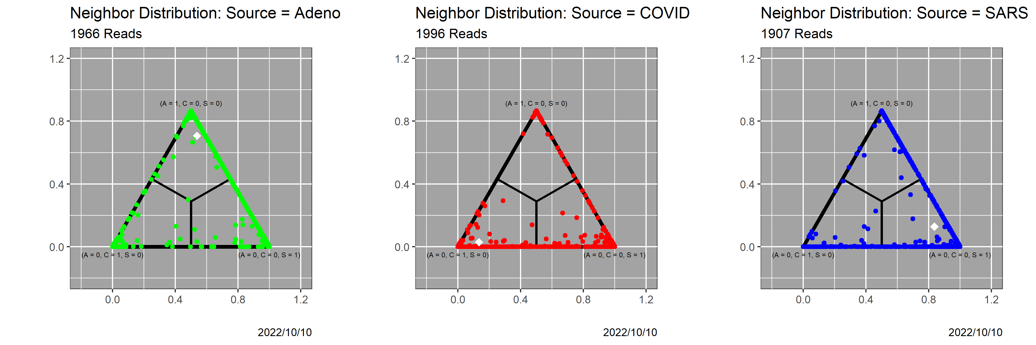
Looking in more detail, Figure 1 shows the neighbor distributions over for all the reads. In it, three-dimensional probabilities (barycentric coordinates) are converted to Cartesian coordinates, as points in an equilateral triangle. Pure Adeno, in the sense that , is the top vertex, pure COVID is the lower left vertex, and pure SARS is the lower right vertex. Because we know the sources of the reads, we create separate displays for each source. The white diamond in each scatterplot is the centroid of the probabilities it contains, and all three centroids lie close to the source. A read on an edge has neighbors of two kinds, one of which is that of the read itself. (In theory, a read could have without neighbors of its same type, but this bizarre case of a read classified differently from all of its neighbors does not occur in our dataset. The minimum number of concordant neighbors is 11.) A read in the interior of the triangle has neighbors with all three decisions.
The topmost table in Table 2 shows Boundary Status as a function of read source, so that its row sums match those in Table 1. The distribution of Boundary Status is not uniform across the three sources: boundary percentages are 30.0% for Adeno reads, 22.1% for COVID reads and 40.0% for SARS reads. The -value for the test on this table is less than , so the differences are significant. SARS reads are more likely than others to lie on the boundary.
The middle table in Table 2 provides a complementary view of Boundary Status as a function of classifier decision, so that its row sums match the column sums in in Table 1. Here also, the test is massively significant. SARS remains the outlier: relatively more reads classified as SARS lie on the boundary than for Adeno or COVID.
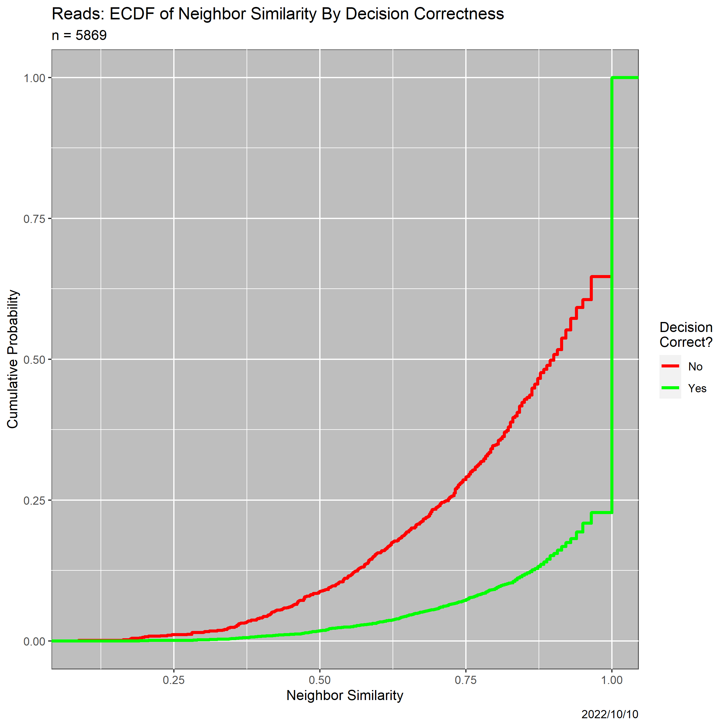
The bottom table in Table 2 shows Boundary Status as a function of correctness of the classifier decision, and begins to get at the heart of the matter. Of incorrectly decided reads, 64.66% lie on the boundary, while only 22.81% of correctly decided reads lie on the boundary! The classifier is struggling in the vicinity of , and one rightly should be less confident of such decisions. The statistic for this table is 726.65, more than five times that for source (topmost table), and three times that for decision (middle table). Moreover, the Kolmogorov-Smirnov test for the two empirical cumulative distribution functions (ECDFs) is massively significant: Boundary Status is higher for incorrect decisions than for correct ones.
| Boundary Status | ||||
|---|---|---|---|---|
| Source | 0 | 1 | 2 | Sum |
| Adeno | 1378 | 526 | 62 | 1966 |
| COVID | 1554 | 375 | 67 | 1996 |
| SARS | 1146 | 700 | 61 | 1907 |
| Sum | 4078 | 1601 | 190 | 5869 |
| Boundary Status | ||||
|---|---|---|---|---|
| Decision | 0 | 1 | 2 | Sum |
| Adeno | 1408 | 491 | 34 | 1933 |
| COVID | 1575 | 345 | 81 | 2001 |
| SARS | 1095 | 765 | 75 | 1935 |
| Sum | 4078 | 1601 | 190 | 5869 |
| Boundary Status | ||||
|---|---|---|---|---|
| Correct? | 0 | 1 | 2 | Sum |
| No | 382 | 598 | 101 | 1081 |
| Yes | 3696 | 1003 | 89 | 4788 |
| Sum | 4078 | 1601 | 190 | 5869 |
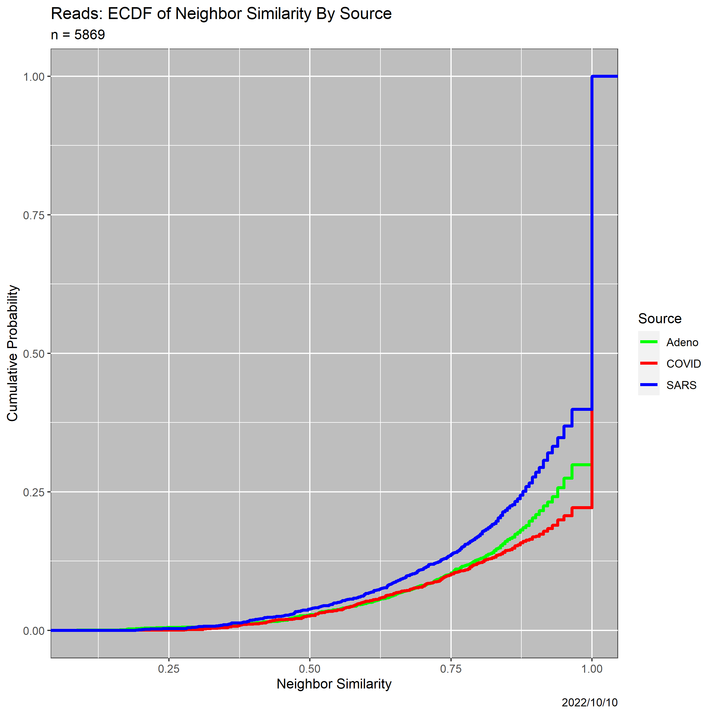
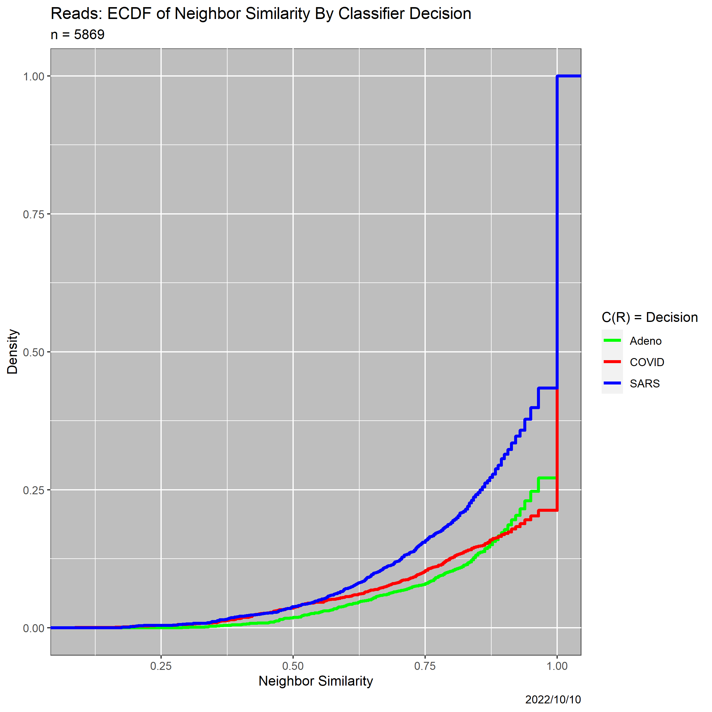
In parallel to Table 2, Figures 2 shows the distribution of Neighbor Similarity as a function of read source, read decision and decision correctness. In particular, these ECDFs make clear how many reads are not on the boundary, for which . The qualitative messages mirror those in Table 2.
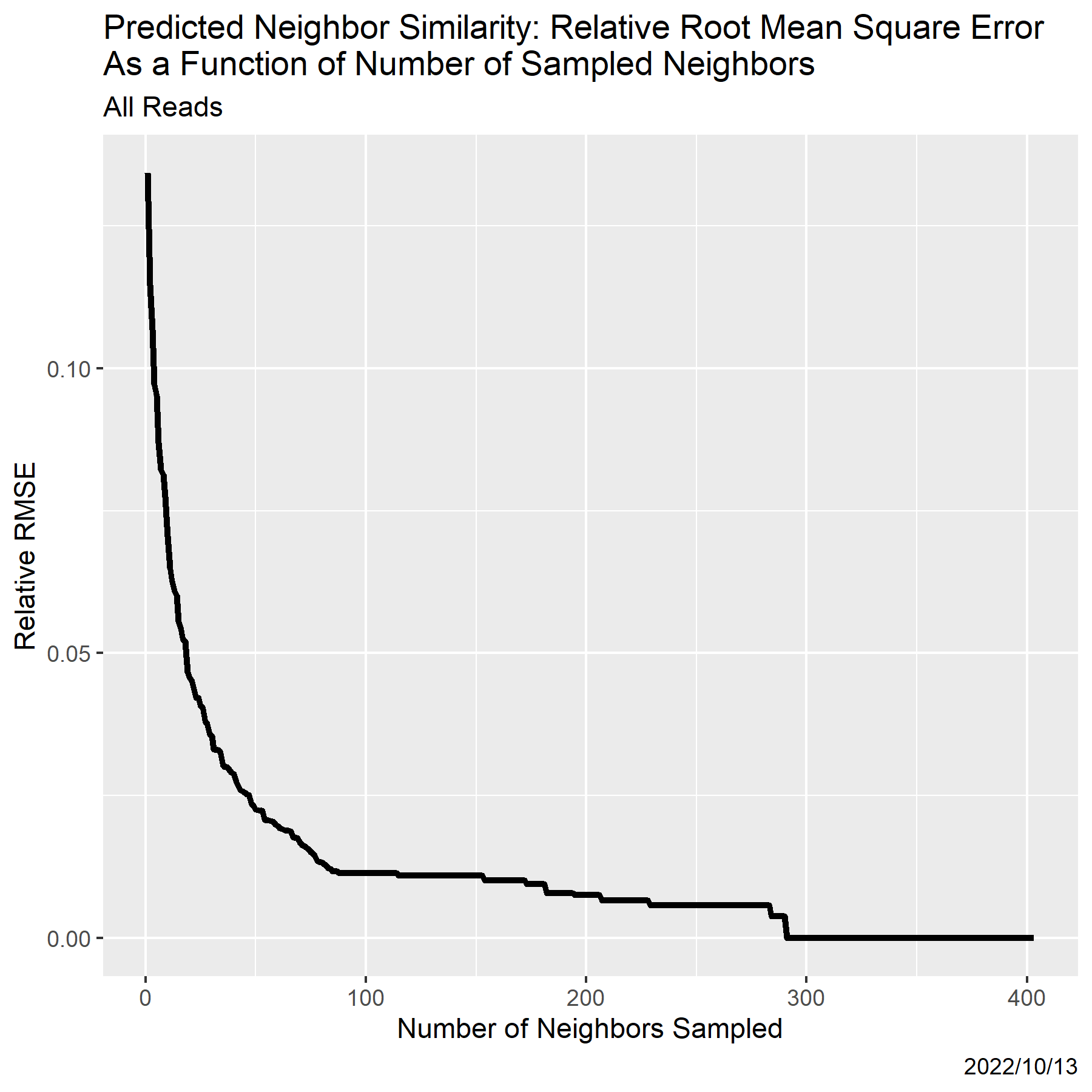
Neighbor Similarity is, obviously, more burdensome computationally than simply running the classifier. However, the computation is infinitely parallelizable: classifier evaluation for one neighbor is completely independent of that for other neighbors. An alternative strategy is to sample neighbors, which generates estimates for Neighbor Similarity. Figure 3 provides initial evidence that sampling can be effective. It is based on the entire 5869-element read dataset. The -axis is the number of reads sampled; the order was randomized for each read. The -axis is more complicated. For each read and sample size we calculated a partial Neighbor Similarity using (6). Then for each , we fitted a linear model with as response and as predictors. Finally, the -axis contains values of relative root mean squared error (RRMSE)888The square root of the mean squared error for the linear model divided by the mean response. for each model. From the figure, an RRMSE of 5% requires only 20 sampled neighbors, and there is minimal benefit from sample sizes exceeding 80. How these values scale with problem size is not clear.
4.2 Relationship to Inherent Measures of Uncertainty
We next investigate the relationships between Neighbor Similarity and the two inherent measures for : —the maximum of the three posterior probabilities, and —the entropy of the posterior distribution. Always, , and the closer is to 1, the more certain is of the decision for . Figure 4 depicts the relationship between MP and NS as a function of classifier decision. Because one ultimate goal is to employ NS in contexts where neither MP nor a model-derived analog is available, it would not have been appropriate to use read source there rather classifier decision. The correlation between MP and NS is ; the disaggregated correlations are 0.8784 for Adeno, 0.8502 for COVID and 0.8400 for SARS.
We can construct good statistical models to predict from and , of which we present two. The first is a fully saturated quadratic model reflecting the curvature evident in Figure 4:
| (8) |
As the notation suggests, the process is equivalent to fitting three separate models to datasets constructed by filtering on . The adjusted coefficient of determination for the model is 0.8341, indicating good fit. Figure 5 shows actual and predicted values of MP by classifier decision. Much of the imperfect fit is simple inability to predict the continuous variable MP within sets of reads having the same value of NS (especially those with ), which the figure makes perfectly clear.
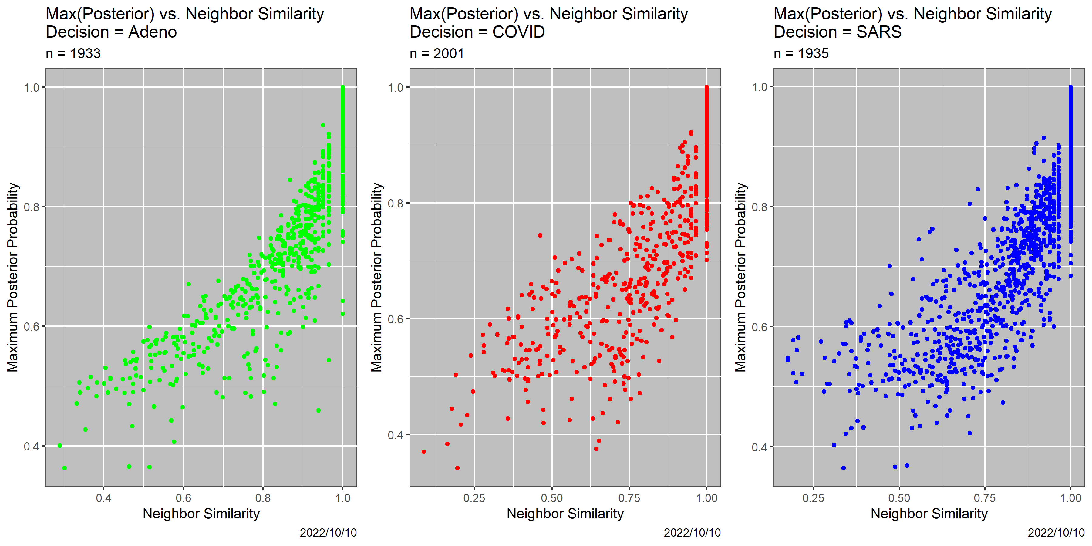
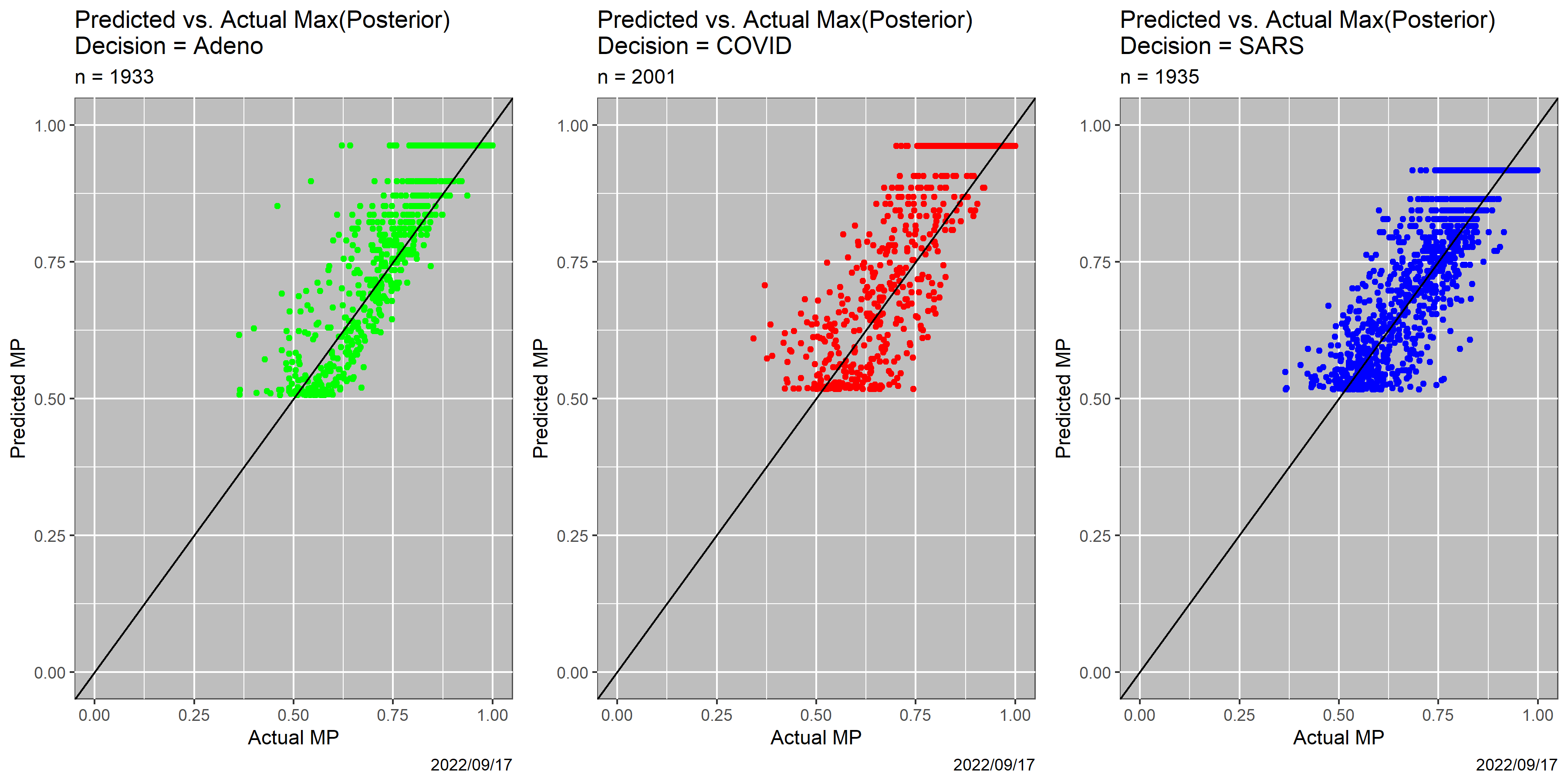
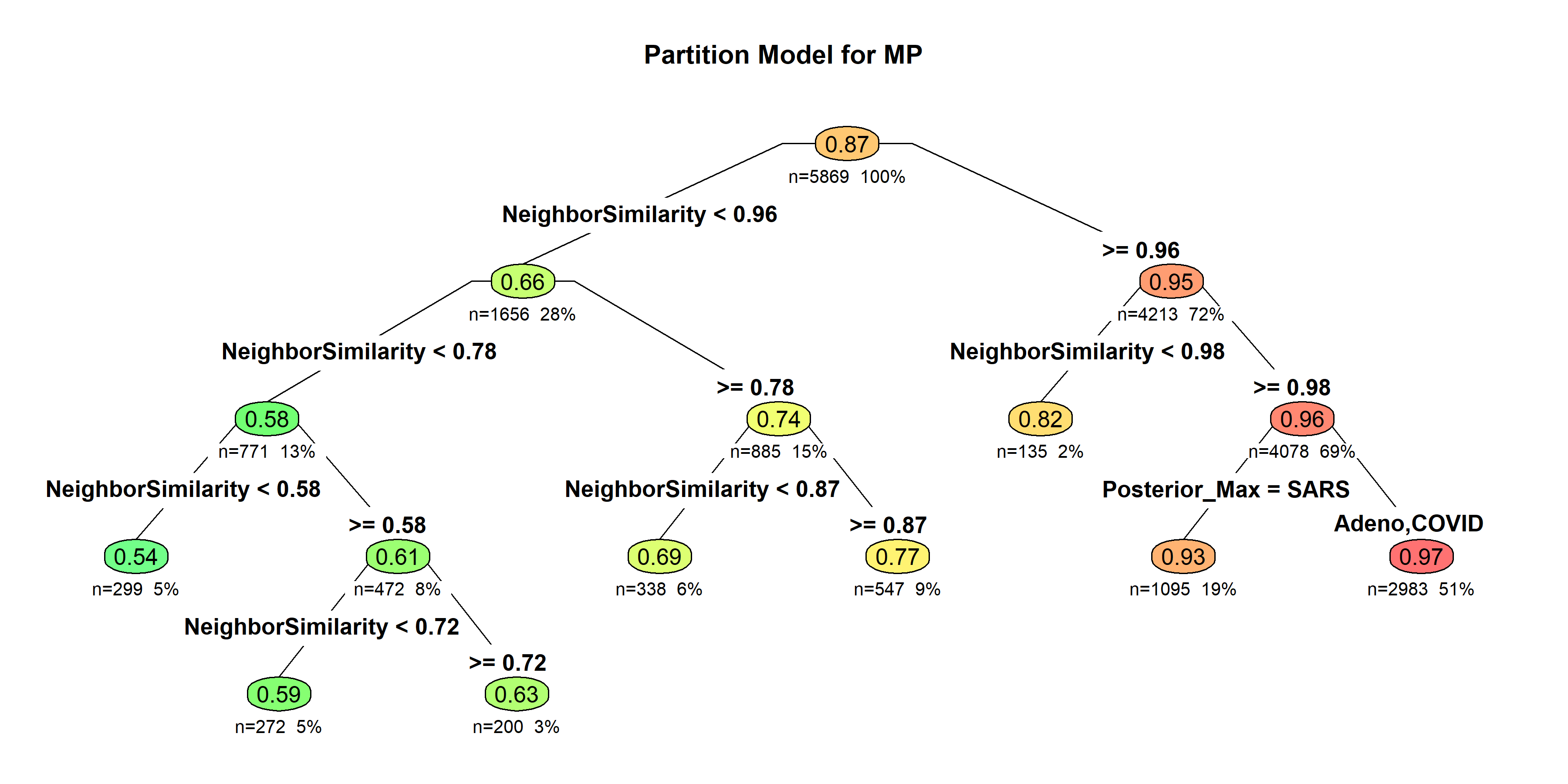
Figure 6 shows a partition model—in this case, a regression tree (Breiman et al.,, 2017; Hastie et al.,, 2001). The tree has been pruned to only seven terminal nodes using standard heuristics that trade off predictive accuracy for model complexity. The mean squared error is slightly superior to that for the regression model—0.003313057 as compared to 0.003794415.
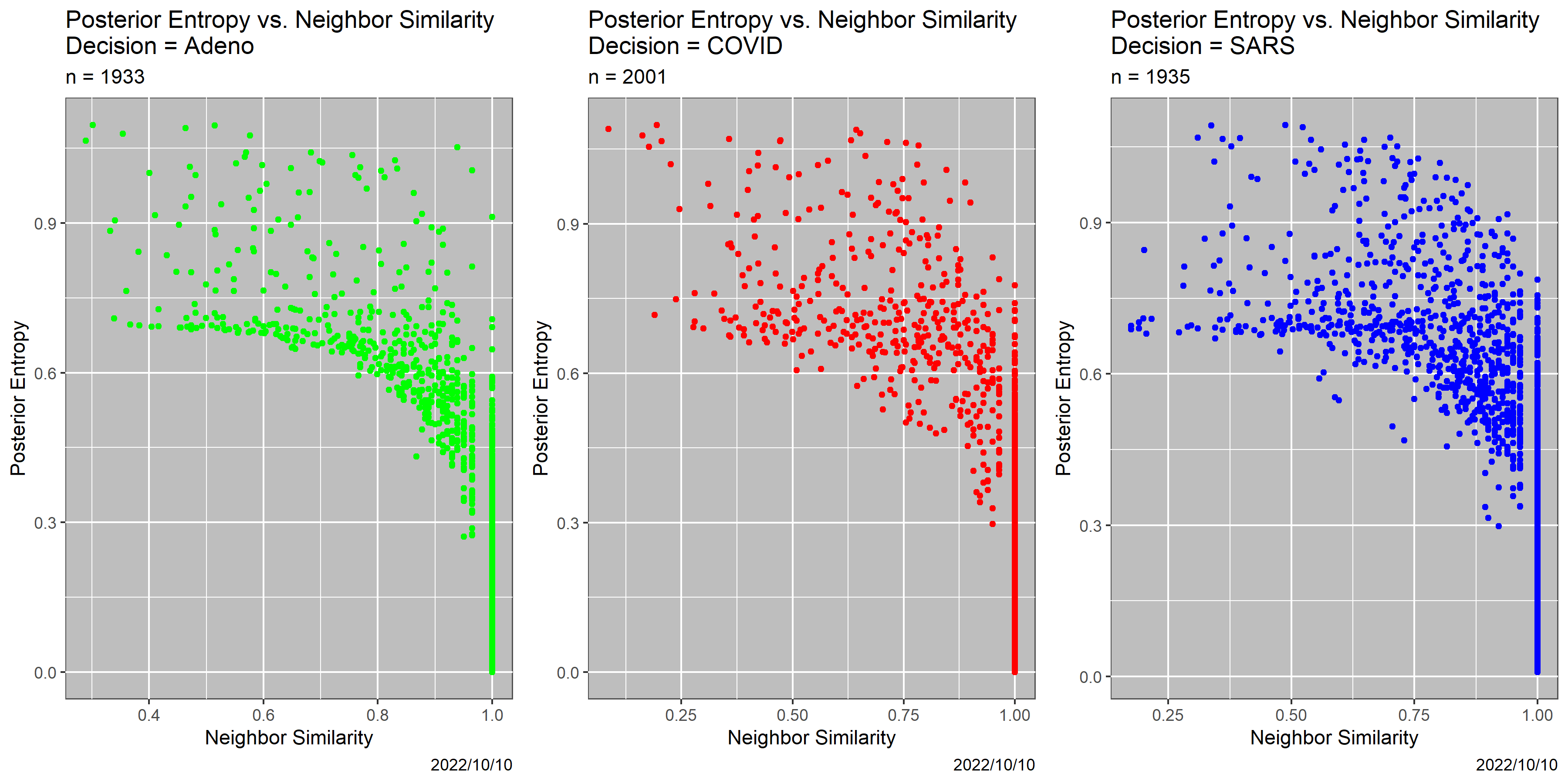
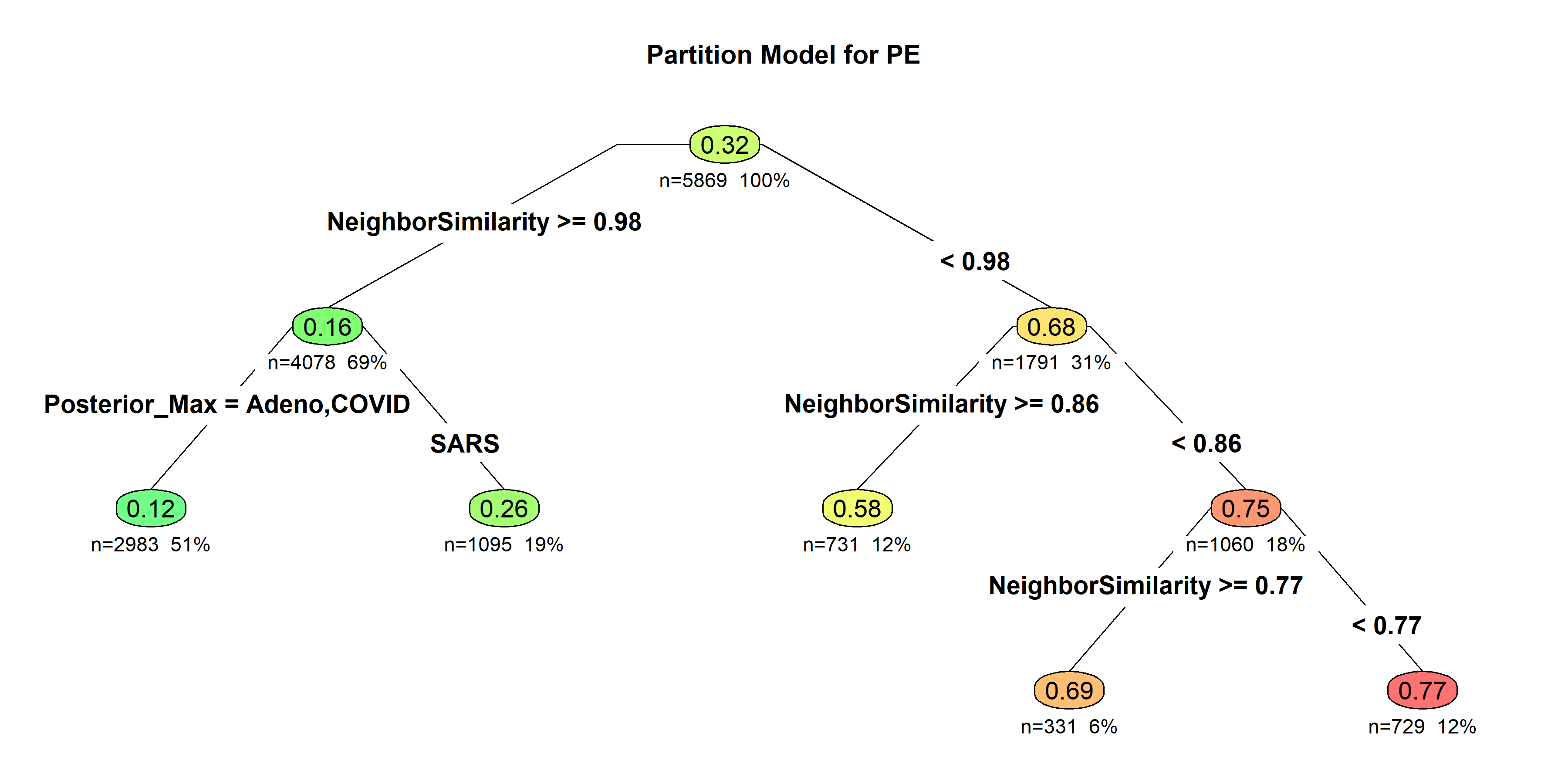
The second inherent measure of uncertainty for is posterior entropy PE. The correlations between NS and PE are -0.7167 (aggregated), -0.7437 (Adeno), -0.7280 (COVID) , and -0.6964 (SARS). Analogously to Figure 4, Figure 7 contains scatterplots of PE versus NS by classifier decision. Clearly, PE is predicted less well by NS and classifier decision than is MP. For a quadratic regression model analogous to that in (8), the adjusted is only 0.6928. The corresponding partition model, shown in Figure 8, identifies which variables and interactions are most relevant. Again, the mean squared error is slightly lower than for the quadratic regression model.
4.3 Exploring the Boundary
We present here three strategies for locating the boundary and exploring its structure.
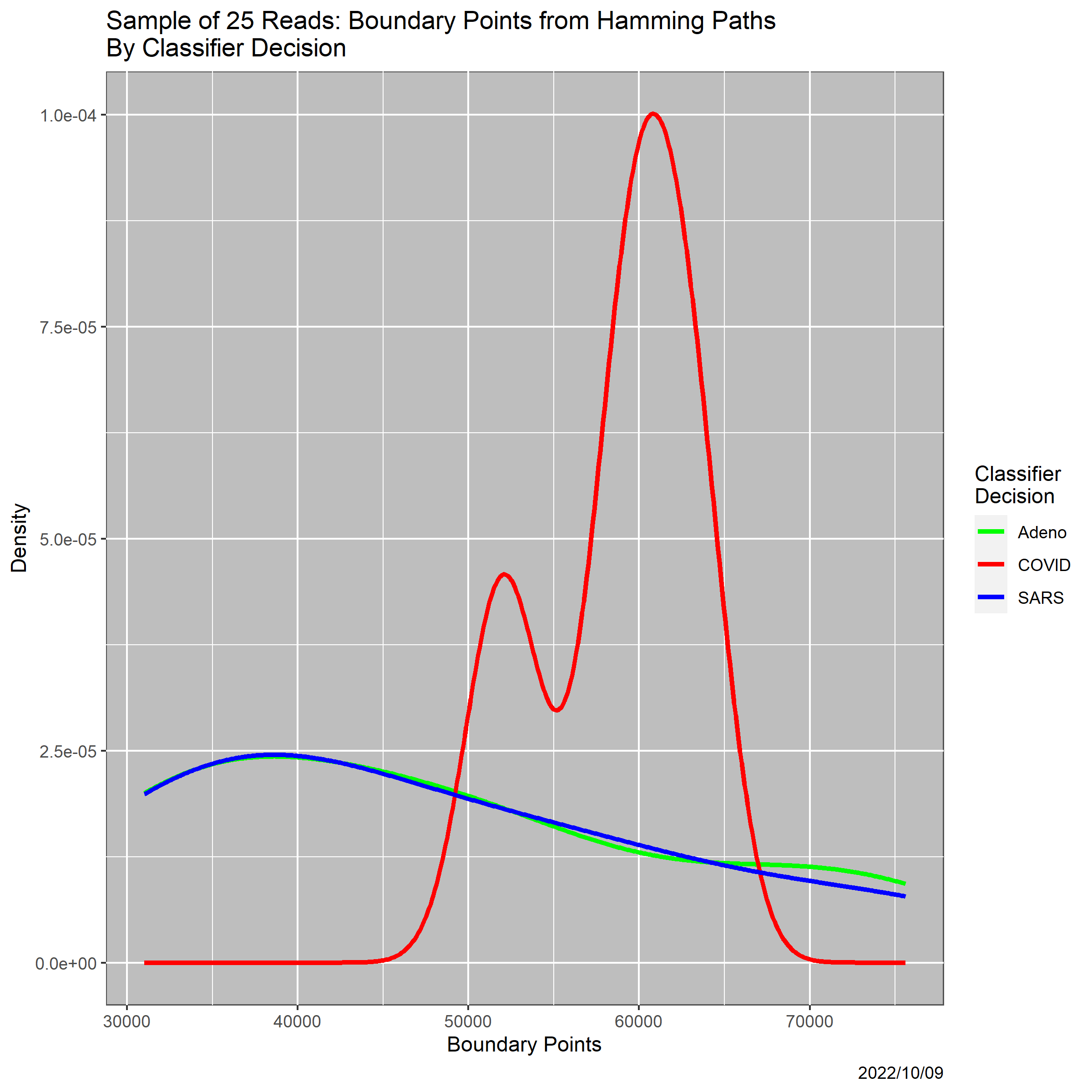
The first and simplest method for locating has been mentioned already in Section 3.1: if , then any path from to contains at least two elements of . Within the reads dataset, there are 11,480,223 such pairs. If we eliminate duplicates and for each pair consider only the Hamming path that in left-to-right order replaces each nucleotide in differing from the corresponding nucleotide in by the latter, then we have a mechanism for locating boundary pairs. Based on a random sample of 25 origin reads, but considering all other reads with different decisions, 1,242,162 boundary points were identified. There is significant variability, however, as shown in Table 3. Moreover, the table shows that paths originating from reads classified as COVID differ significantly from those originating at reads classified as Adeno or SARS.
| SampleID | Decision | Boundary Points | Classifier Evaluations |
|---|---|---|---|
| 958 | Adeno | 71646 | 296286 |
| 1283 | SARS | 59530 | 298994 |
| 256 | Adeno | 50388 | 294923 |
| 1137 | SARS | 32052 | 303790 |
| 638 | SARS | 75160 | 296341 |
| 4905 | Adeno | 57804 | 302409 |
| 2914 | Adeno | 42374 | 292198 |
| 513 | COVID | 63228 | 289336 |
| 2160 | COVID | 52038 | 292711 |
| 2835 | COVID | 58806 | 293286 |
| 1386 | Adeno | 31784 | 304305 |
| 3584 | Adeno | 40992 | 296839 |
| 1912 | SARS | 34274 | 296172 |
| 4857 | Adeno | 31002 | 302553 |
| 3713 | Adeno | 37630 | 292638 |
| 4196 | Adeno | 32332 | 300289 |
| 5113 | Adeno | 68118 | 293587 |
| 4090 | SARS | 43252 | 297002 |
| 1981 | Adeno | 49500 | 293600 |
| 2666 | Adeno | 50380 | 295404 |
| 2153 | COVID | 60832 | 295370 |
| 2674 | SARS | 52446 | 295611 |
| 351 | Adeno | 75608 | 301328 |
| 5154 | SARS | 37546 | 297293 |
| 1940 | Adeno | 33440 | 303009 |
Of course, whenever , there are multiple Hamming paths connecting and . Initial experiments have shown that a strategy of using multiple Hamming paths is not materially more effective than using one Hamming path in terms of unique boundary pairs identified relative to computational effort. The reason, we hypothesize, is that multiple paths from to often cross at the same places.
A second strategy, motivated by Markov chain Monte Carlo (MCMC) methods used to investigate large spaces of contingency tables (Diaconis and Sturmfels,, 1998), is to perform random walks originating from sequences , moving to a neighboring sequence at each step, and checking whether has been crossed, i.e., whether the classifier decision has changed. Were thin, this strategy of wandering randomly would be horribly ineffective. But, because is not thin, it works reasonably well. To illustrate, we chose a random sample of 100 reads for each decision, and ran random walks of length 2000 steps originating at each. Keeping in mind that each boundary pair comprises two boundary points, 35,352 boundary points were found, of 600,300 sequences visited.
The hypothesis that this process would be more efficient if started from a boundary point is not confirmed. We repeated the experiment starting from 300 sequences known to be boundary points, again spread uniformly over the three decisions. The improvement over random walks starting from random sequences is minimal; indeed, fewer boundary points—35,238—were identified. We interpret this as further confirmation that the boundary is not thin, so that starting from it generates little benefit. Note that none of the 600 random walks failed to cross the boundary, so it is never far away. Summary statistics appear in Table 4.
| Origins | Minimum | Mean | Maximum |
|---|---|---|---|
| Reads | 28 | 117.77 | 274 |
| Boundary Points | 16 | 117.46 | 280 |
From Table 5, both versions of random walks are less efficient than Hamming paths, as measured by the number of boundary points identified divided by the number of classifier evaluations, which is the primary computational expense of boundary exploration. But, these results again confirm the omnipresence of .
Note that in our implementation both Hamming paths and random walks may pass through boundary points without identifying them, which can happen because, for computational efficiency, each point in the path is compared only to its predecessor rather than all of its neighbors.
Finally, we present random walk-like methods for “crawling the boundary” once it has been reached. We simulated 100 random walks starting at boundary points, but constrained to move only to adjacent and not previously visited boundary points. Each crawl was allowed to continue for 250 steps, or until it was not possible to move to another and not previously visited boundary point. The fact that such points exist further confirms the geometric complexity of the boundary: it is ”hairy” in the sense that the points from which no continuation is possible are tips of hairs.
Crawling the boundary, while insightful, is not efficient. Of the 100 random walks, 64 did not terminate within 250 steps, indicating that the boundary is significantly contiguous. The lengths of crawls that did terminate range from 5 to 242, with no discernible structure to their distribution. The 36 crawls that did terminate are the hairs mentioned in the preceding paragraph—points at which continuing on the boundary is possible only by backtracking. While in the minority, they are nevertheless not rare. Beyond this, the boundary is convoluted: all three decisions are present in 58 of the 100 crawls. Put differently, if one were to think of three boundaries—an Adeno–COVID boundary, an Adeno–SARS boundary, and a COVID–SARS boundary—they cross each other frequently, as evidenced by the 190 reads with neighbors of all three types. In all other crawls, the decisions must and do alternate, indicating that some segments of the boundary lie between two decisions.
The inefficiency of crawling the boundary, which is apparent in Table 5, is partly an artifact of our computational implementation. At each step, we classify all neighbors before determining if it is possible to proceed. Computation would be reduced by examining neighbors sequentially, and proceeding once a neighbor with a differing classification is identified.
| Method | Classifier Evaluations | Boundary Points | Efficiency |
|---|---|---|---|
| Hamming Paths | 7,425,274 | 1,242,162 | 16.73% |
| Random Walks, Random Origin | 600,300 | 34,932 | 5.82% |
| Random Walks, Boundary Origin | 600,300 | 25,238 | 5.87% |
| Crawling Boundary | 8,146,256 | 20,164 | 0.25% |
4.4 Do Boundary Points Differ from Other Reads?
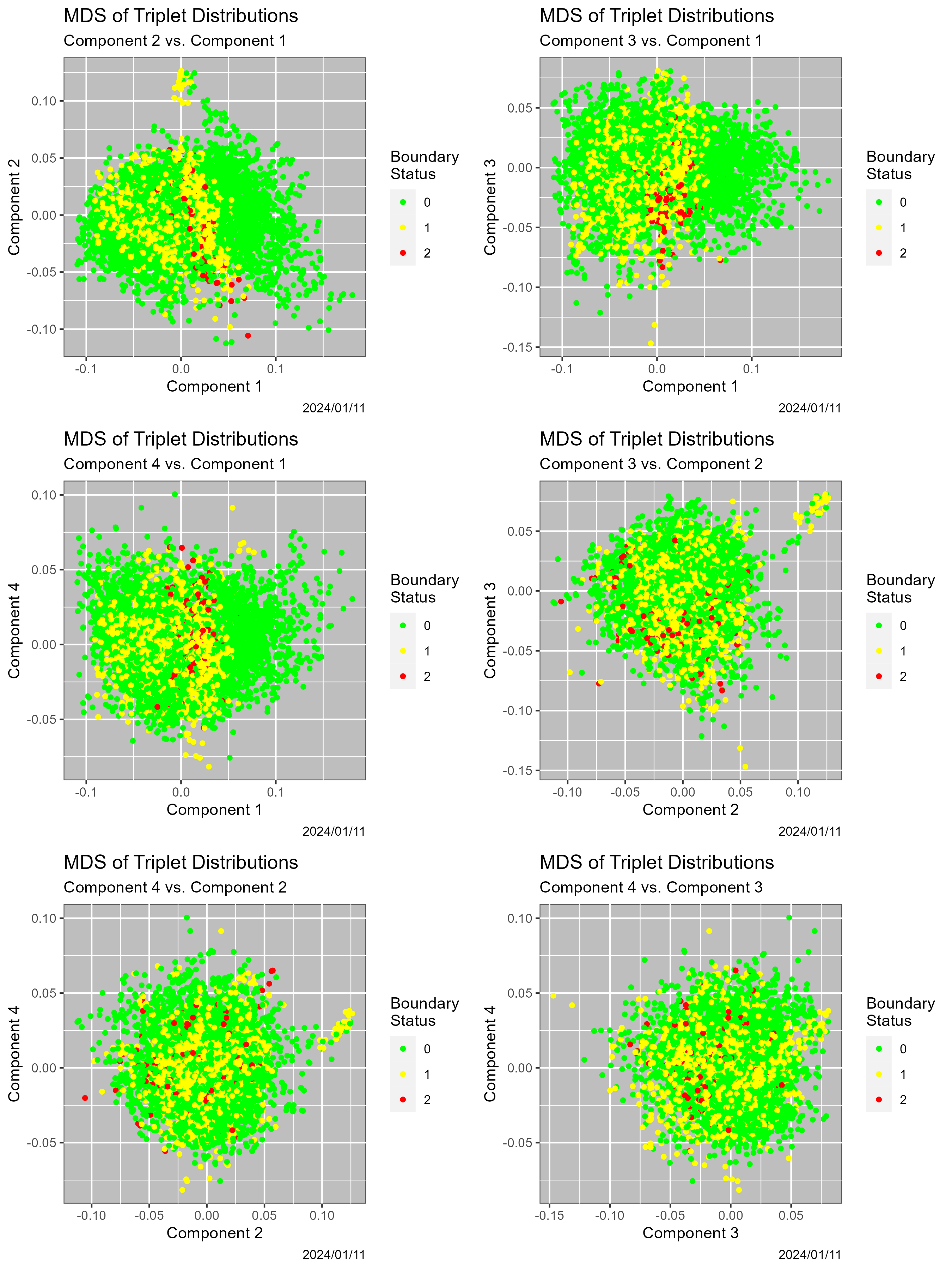
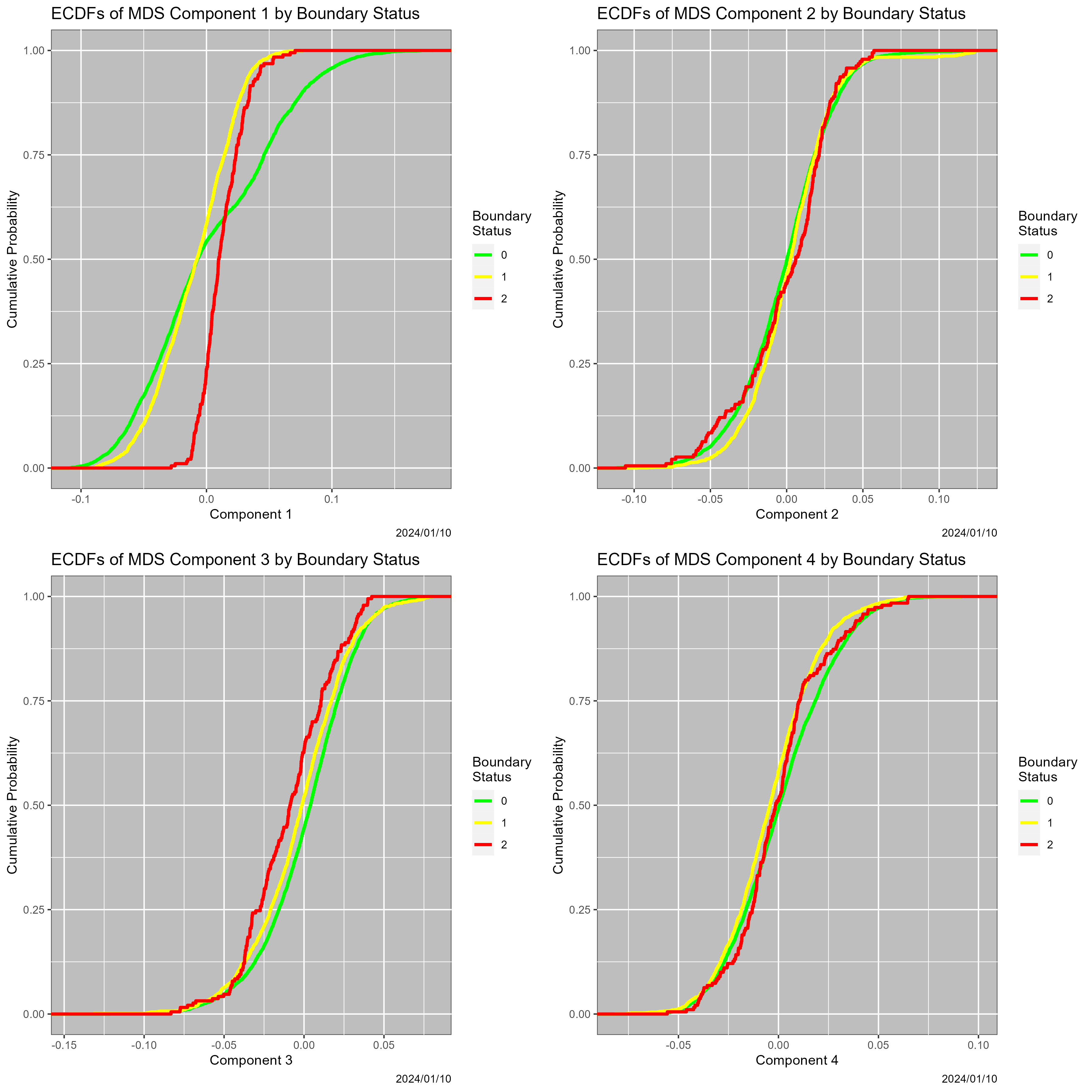
Our final results address a natural question: do the 1791 boundary reads in our dataset differ from the 4078 other reads? Figure 10 provides initial insight. It contains scatterplots of the four components of a multi-dimensional scaling (MDS) (Kruskal and Wish,, 1978) of the triplet distributions, colored by Boundary Status. The most striking feature is the concentration of values of Component 1 for reads with , which is reinforced by the upper left-hand panel in Figure 11. This latter figure contains plots of the ECDFs of each of the four components, disaggregated by Boundary Status; the colors match those in Figure 10. In fact because of overplotting in Figure 10, there is additional structure that is less visible in it than in Figure 11. Notably, there are many instance where one ECDF lies entirely below another, including Component 1 () below Component 1 (); effectively, Component 3 () below Component 3 () below Component 3 (); Component 4 () below Component 4 (); and Component 4 () below Component 4 (). Almost uniformly the differences among the ECDFs, as evaluated by Kolmogorov-Smirnov tests, are statistically significant.
A partition model with triplet distributions as predictors and BS as response tells a complementary story. Without pruning, the model has 818 terminal nodes, with sizes ranging from 1 to 296, and predicts Boundary Status exactly. When the model is pruned with standard heuristics, there are 705 nodes ranging in size from 1 to 347, with the confusion matrix shown in shown in Table 6. The correct classification rate is 98.76%.
Many analysts would still be uncomfortable that this model is overfit, so in Table 7, we show all possible pruned versions of the model, as generated by the R package rpart. At the top is the “default model” that predicts all reads to have Boundary Status 0. At the bottom is the unpruned, and perfect, model. Halving the incorrect classification rate from 30% to 15%, for instance, requires only 182 terminal nodes. Their sizes range from 3 to 445, with a mean size of 32 and median of 14. To demonstrate the scientific insights that follow from this approach, Table 10, in Appendix B, shows the importance of each of the 64 predictors to the splits that comprise the model, as percentages that sum to 100%. In order, the five most important predictors are TTT (which codes for the amino acid phenylalanine), TAT (tyrosine), GTT (valine), GCG (alanine), and AAG (lysine).
Finally, regarding validation, if the 705-node pruned model is applied to the 6000-element ReadsNew dataset discussed in Section 5.2.1, it correctly predicts Boundary Status in 4464 cases, or 74.2%, which is respectable performance given the limited training data.
| Predicted | ||||
|---|---|---|---|---|
| Actual | 0 | 1 | 2 | Sum |
| 0 | 4061 | 17 | 0 | 4078 |
| 1 | 49 | 1552 | 0 | 1601 |
| 2 | 4 | 3 | 183 | 190 |
| Sum | 4114 | 1572 | 183 | 5869 |
| Complexity Parameter | Terminal Nodes | Correct Classification Rate |
|---|---|---|
| 0.004467 | 1 | 69.483728 |
| 0.003908 | 35 | 74.646447 |
| 0.003350 | 41 | 75.413188 |
| 0.003210 | 42 | 75.515420 |
| 0.002792 | 49 | 76.299199 |
| 0.002606 | 61 | 77.321520 |
| 0.002513 | 65 | 77.645255 |
| 0.002233 | 74 | 78.394957 |
| 0.002171 | 110 | 80.882604 |
| 0.002122 | 123 | 81.802692 |
| 0.002047 | 128 | 82.126427 |
| 0.001954 | 131 | 82.313852 |
| 0.001861 | 140 | 82.859090 |
| 0.001675 | 143 | 83.029477 |
| 0.001535 +++ | 182 | 85.244505 |
| 0.001489 | 189 | 85.619356 |
| 0.001396 | 204 | 86.300903 |
| 0.001303 | 214 | 86.726870 |
| 0.001196 | 223 | 87.084682 |
| 0.001117 | 232 | 87.425456 |
| 0.000977 | 357 | 91.906628 |
| 0.000931 | 364 | 92.128131 |
| 0.000838 | 375 | 92.468904 |
| 0.000782 | 410 | 93.388993 |
| 0.000744 | 420 | 93.678651 |
| 0.000698 | 441 | 94.223888 |
| 0.000558 | 445 | 94.309082 |
| 0.000465 *** | 705 | 98.756177 |
| 0.000419 | 712 | 98.858409 |
| 0.000372 | 724 | 99.028795 |
| 0.000279 | 773 | 99.625149 |
| 0.000186 | 815 | 99.982961 |
| 0.000000 | 818 | 100.000000 |
5 Discussion
There are two themes in this paper: the nature of the boundary and the surrogate measures of uncertainty based on the boundary, especially Neighbor Similarity. Concerning the former, the takeaway message is “beware the boundary.” For our Bayes classifier, all of our analyses suggest that the boundary may comprise 20% or more of the input space. The boundary is both not sparse and geometrically complicated.
5.1 General Issues
The extent to which lying on or near the boundary can or should affect either classifier output or decisions based on it is clearly contextual. The first issue is whether to check boundary status for a given query. So long as the input space has graph structure, the issue is computational, not conceptual: simply check all the neighbors, which, as noted, is completely parallelizable. If one cares only about whether the query is on the boundary, the process can be terminated once a neighbor with a different result is found. However, given the size of the boundary, this strategy is almost surely too blunt. In many cases, both scientific and broader impacts merit a quantified measure such as Neighbor Similarity. Although in our read classification case study, the consequences of misclassification are not major, for classifiers such as SeqScreen (Balaji et al.,, 2022), which is designed to identify pathogenic sequences, the consequences of incorrect decisions may be dramatic, and the risks of accepting high-uncertainty classifier results without further investigation may be unacceptable. Not knowing the level of uncertainty is equally problematic.
Furthermore, in the face of rampart concern about data quality in DNA databases (Commichaux et al.,, 2021; Langdon,, 2014; Steinegger and Salzberg,, 2020), and given that changing a data point to a neighbor, as done in (Karr et al.,, 2022) to measure data quality, is seemingly the most innocuous data quality problem,999As least with respect to the accuracy dimension of data quality, which is but one of many dimensions (Karr et al.,, 2006). it seems prudent to care about neighbors.
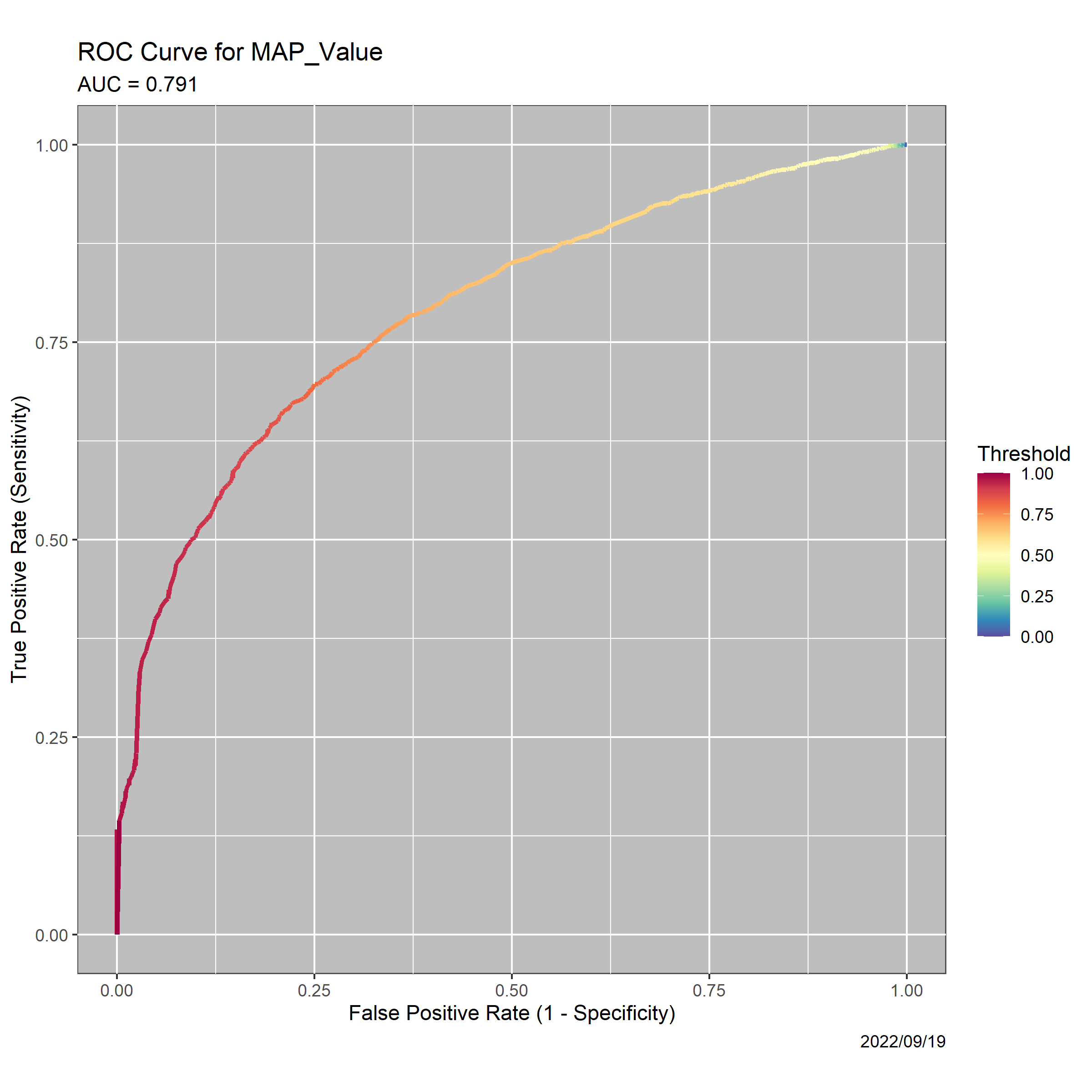
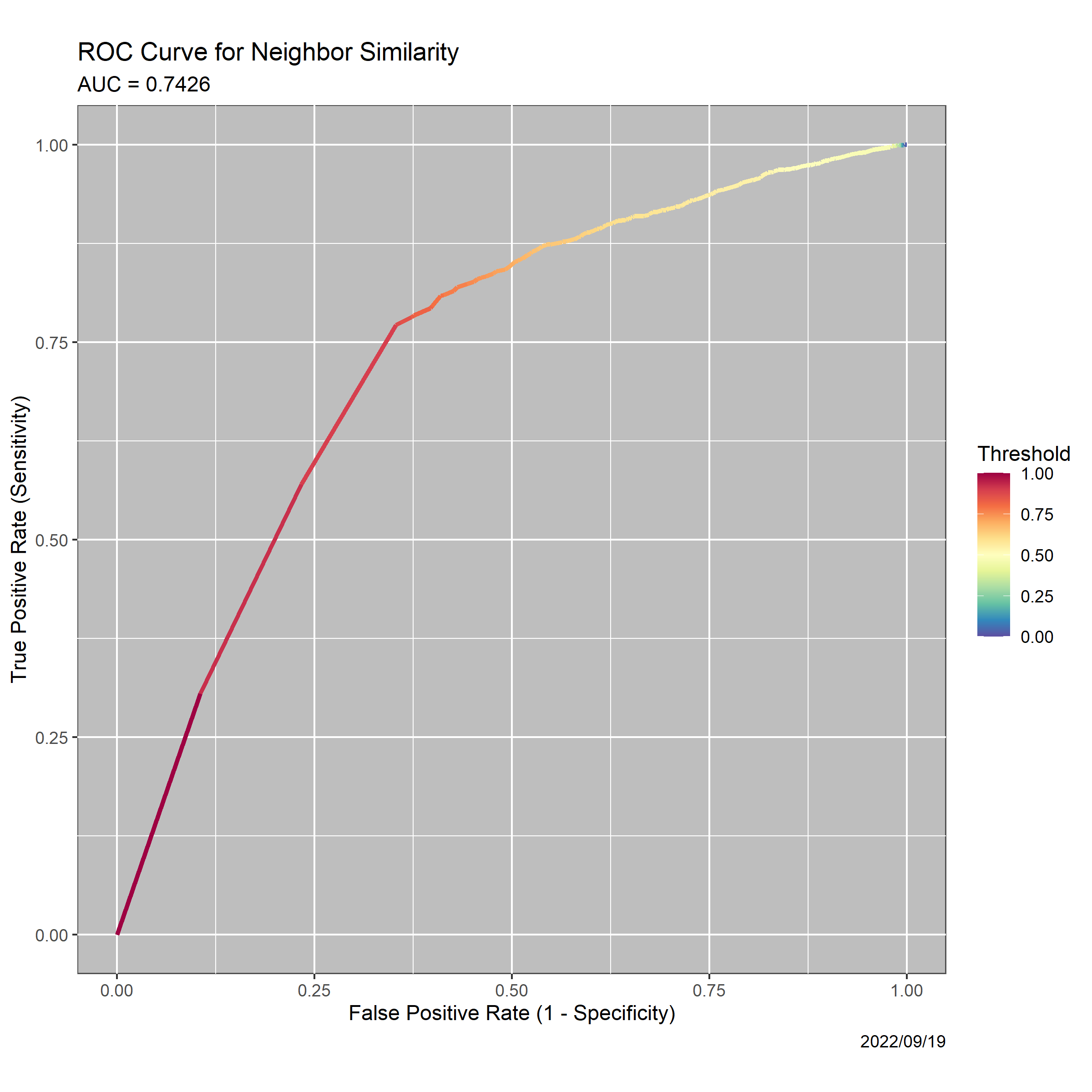
In Section 4, we showed that that Neighbor Similarity relates to both inherent measures of uncertainty for our Bayes classifier. From an operational perspective, Figure 12 is more important. It contains receiver operating characteristic (ROC) curves for two decision rules, one based on accepting decisions for which MAP exceeds a threshold, which is encoded by color, the other for the decision rule based on accepting decisions for which NS exceeds a threshold. The two ROC curves are essentially identical. For the Bayes classifier, NS is as effective as MAP for making principled decisions.
5.2 Scientific Generalizability
There are, of course, questions of scientific generalizability: are the properties observed somehow specific to our read dataset, or descriptive of the classifier more generally? And do they apply to other classifiers?
5.2.1 Other Datasets
To address the first question, we ran the classifier on five additional datasets:
- ReadsNew:
-
A dataset containing 2000 Adeno reads, 2000 COVID reads and 2000 SARS reads, all of length 101, generated by the Mason_simulator, which can be viewed as addressing the question of replicate variability. There is no reason to expect the classifier to perform differently on it than on the main dataset.
- ReadsEcoli:
-
A dataset containing 6000 Mason_simulator-generated reads of length 101 from an E. coli genome.
- Random6K:
-
A dataset containing 6000 random sequences of length 101 generated from A, C, G, T, which represents pure noise.
- ReadsMixed1:
-
A dataset combining the original dataset and 2000 elements of ReadsEcoli, which represents a situation that the classifier is not prepared for: the presence of a fourth source of reads.
- ReadsMixed2:
-
A dataset combining the original dataset and 100 elements of ReadsEcoli, which represents an alternative situation that the classifier is not prepared for: contamination from a fourth source of reads.101010Contamination of DNA samples is a pervasive problem in multiple contexts, especially analysis of ancient DNA (Reich,, 2018).
The results, including the core dataset ReadsOriginal for comparison, appear in Table 6 and Figure 13. In Table 6, the three columns under “Decisions” are percentages of the classifier output, as are the two columns under “Boundary.” The first two rows, representing two sets of reads from Adeno, COVID and SARS with approximately equal distributions of the read source, do not differ, meaning the that classifier seems not to be vulnerable to replicate variability. The last two rows differ the most from ReadsOriginal, and both the Decision distribution and the Boundary distribution differ dramatically from the first two rows. For reasons that are not yet clear, ReadsEcoli and Random6K are overwhelmingly classified as Adeno. The hypothesis that this constitutes a “vote splitting” artifact of there being one Adenovirus genome and two Coronavirus genomes is demonstrably false. In a set of 30,000 random sequences, if classifier choices are restricted to Adeno and Corona, only 77 of the 27,492 sequences classified as Adeno change to the latter. But ReadsEcoli and Random6K also differ: using Hellinger distances and empirical -values, the differences between the Decision distributions and Boundary distributions are massively significant.
The third and fourth rows in Table 6 are, as expected, midway between the first two rows and the last two rows. Note that, for ease of interpretation, row 3 contains ReadsMixed2—the case with 100 contaminating E. coli reads, which should be, and is, closer to ReadsOriginal and ReadsNew than ReadsMixed1, with 2000 E. coli reads.
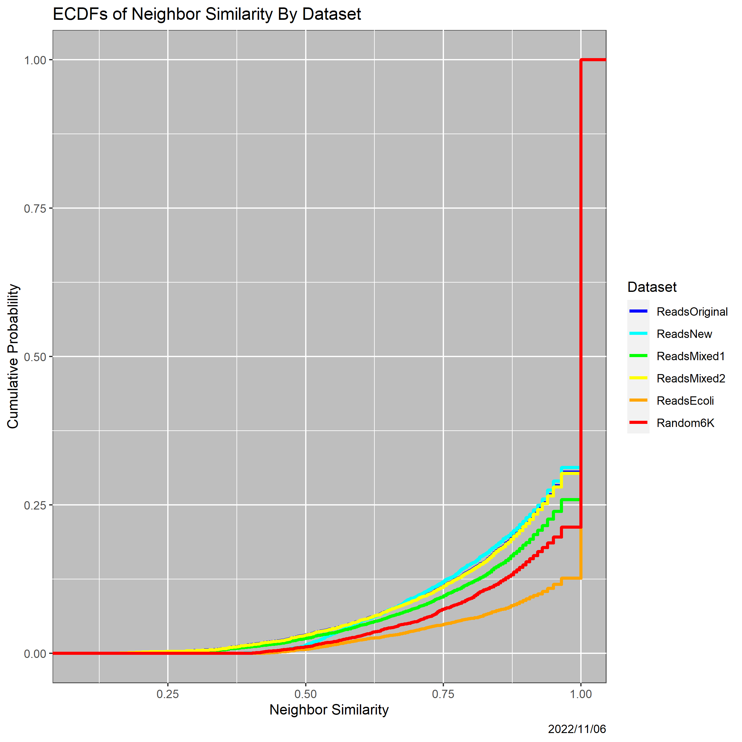
Figure 13 contains the ECDFs of Neighbor Similarity for all six datasets. That for ReadsOriginal (blue) is essentially completely overplotted by those for ReadsNew (cyan) and ReadsMixed2 (green). Interestingly, but consistent with the Boundary columns in Table 6, ReadsEcoli is now the most different from ReadsOriginal, ReadsNew and ReadsMixed2, even though it contains “real” reads. We performed one- and two-sided Kolmogorov-Smirnov tests on selected pairs of the ECDFs in Figure 13. No difference involving ReadsOriginal, ReadsNew and ReadsMixed2 was remotely significant. On the other hand, differences between ReadsOriginal and all of ReadsMixed1, Random6K, and ReadsEcoli were massively significantly, in the latter two cases with -values of zero.
Therefore, Boundary Status and Neighbor Similarity are usable as diagnostics that indicate when a classifier is being used on data that differ from what was expected. For the Bayes classifier, “what is expected” is incorporated in the prior and the likelihood functions (Karr et al.,, 2023). For many other classifiers, the training data represent “what is expected.” The question is being investigated.
| Decision | Boundary | |||||
|---|---|---|---|---|---|---|
| Dataset | Count | Adeno | COVID | SARS | No | Yes |
| ReadsOriginal | 5869 | 32.94 | 34.09 | 32.97 | 69.48 | 30.52 |
| ReadsNew | 6000 | 32.43 | 33.82 | 33.75 | 68.7 | 31.3 |
| ReadsMixed2 | 5969 | 33.86 | 33.59 | 32.55 | 69.69 | 30.31 |
| ReadsMixed1 | 7869 | 48.1 | 26.2 | 25.7 | 74.1 | 25.9 |
| ReadsEcoli | 6000 | 92.767 | 2.933 | 4.300 | 87.35 | 12.65 |
| Random6K | 6000 | 90.8333 | 0.3833 | 8.7833 | 78.75 | 21.25 |
5.2.2 Other Classifiers
Full results will be reported in forthcoming papers, but initial experiments show similar behavior for other classifiers applied to the same dataset, including partition models, random forests and neural networks.
6 Conclusions
The two principal contributions of this paper are surrogate measures of uncertainty for classifiers and methods for investigating their boundaries. In particular, we propose Neighbor Similarity as a measure of uncertainty for classifiers lacking inherent measures of uncertainty. Despite the computational burden, the potential to avoid incorrect decisions is enormous.
As always, at least as many questions are raised as answered. One of the more challenging is whether Neighbor Similarity is viable in the context of production-grade classifiers such as SeqScreen. A central issue may be whether the information gained justifies the computational cost. A (still short) DNA sequence of length 10,000 has more than 40,000 neighbors, and running SeqScreen on all of them may be prohibitive. We showed the potential of sampling to estimate Neighbor Similarity from a subset of neighbors; investigating demonstrably effective strategies to do so is a priority.
Underlying everything is a scientific and statistical issue not addressed in this paper and clearly needing more attention. Is a low value of a statement about the read or about the classifier? Or, if present, the training data? As long there is a range of observed values of NS, and especially if there are values near 1, then low values are plausibly statements about reads. On the other hand, uniformly small values of seem to suggest problems with the classifier (or, if present, the training data). But then, what if the problem is just innately hard?
Acknowledgements
This research was supported in part by NIH grant 5R01AI100947–06, “Algorithms and Software for the Assembly of Metagenomic Data,” to the University of Maryland College Park (Mihai Pop, PI). We thank Professor Pop for numerous insightful discussions.
References
- Baera et al., (2021) Baera, B. R., Gaudinob, M., Charlson, M., Fremes, S. E., and Wells, M. T. (2021). Fragility indices for only sufficiently likely modifications. Proceedings of the National Academy of Sciences, 118(49):1–12.
- Balaji et al., (2022) Balaji, A., Kille, B., Kappell, A. D., Godbold, G. D., Diep, M., Elworth, R. A. L., Z., Albin, Q. D., Nasko, D. J., Shah, N., Pop, M., Segarra, S., Ternus, K. L., and Treangen, T. J. (2022). SeqScreen: accurate and sensitive functional screening of pathogenic sequences via ensemble learning. Genome Biology, 23:133.
- Breiman et al., (2017) Breiman, L., Friedman, J., Olshen, R., and Stone, C. J. (2017). Classification and Regression Trees. CRC Press, Boca Raton, FL.
- Cepeda et al., (2017) Cepeda, V., Liu1, B., Almeida, M., Hill, C. M., Treangen, T. J., and Pop, M. (2017). MetaCompass: Reference-guided assembly of metagenomes. Preprint, bioRxiv, https://doi.org/10.1101/212506.
- Commichaux et al., (2021) Commichaux, S., Shah, N., Ghurye, J., Stoppel, A., Goodheart, J. A., Luque, G. G., Cummings, M. P., and Pop, M. (2021). A critical assessment of gene catalogs for metagenomic analysis. Bioinformatics. btab216.
- Diaconis and Sturmfels, (1998) Diaconis, P. and Sturmfels, B. (1998). Algebraic algorithms for sampling from conditional distributions. Ann. Statist., 26:363–97.
- Hastie et al., (2001) Hastie, T., Tibshirani, R., and Friedman, J. (2001). The Elements of Statistical Learning: Data Mining, Inference, and Prediction. Springer–Verlag, New York.
- Holtgrewe, (2010) Holtgrewe, M. (2010). Mason: A read simulator for second generation sequencing data. Technical Report FU Berlin.
- Karr et al., (2022) Karr, A. F., Hauzel, J., Porter, A. A., and Schaefer, M. (2022). Measuring quality of DNA sequence data via degradation. PLoS ONE, 2022:0221459. DOI: 10.1371/journal.pone.0221459.
- Karr et al., (2023) Karr, A. F., Hauzel, J., Porter, A. A., and Schaefer, M. (2023). Application of Markov structure of genomes to outlier identification and read classification. Preprint. arXiv:2112.13117.
- Karr et al., (2006) Karr, A. F., Sanil, A. P., and Banks, D. L. (2006). Data quality: A statistical perspective. Statistical Methodology, 3(2):137–173.
- Kruskal and Wish, (1978) Kruskal, J. B. and Wish, M. (1978). Multidimensional Scaling. SAGE, New York.
- Langdon, (2014) Langdon, W. B. (2014). Mycoplasma contamination in the 1000 genomes project. BioData Mining, 7:3.
- Navarro, (2001) Navarro, G. (2001). A guided tour to approximate string matching. ACM Computing Surveys, 33(1):31–88.
- Nikulin, (2001) Nikulin, M. S. (2001). Hellinger distance. In Encyclopedia of Mathematics. EMS Press, Berlin.
- Pride et al., (2003) Pride, D. T., Meinersmann, R. J., Wassenaar, T. M., and Blaser, M. J. (2003). Evolutionary implications of microbial genome tetranucleotide frequency biases. Genome Research, 13:145–158.
- R Core Team, (2020) R Core Team (2020). R: A Language and Environment for Statistical Computing. R Foundation for Statistical Computing, Vienna, Austria.
- Reich, (2018) Reich, D. (2018). Who We Are and How We Got Here: Ancient DNA and the New Science of the Human Past. Vintage Books, New York.
- Steinegger and Salzberg, (2020) Steinegger, M. and Salzberg, S. L. (2020). Terminating contamination: large-scale search identifies more than 2,000,000 contaminated entries in GenBank. Genome Biology, 21(1):115.
- (20) Teeling, H., Meyerdierks, A., Bauer, M., Amann, R., and Glöckner, F. O. (2004a). Application of tetranucleotide frequencies for the assignment of genomic fragments. Environmental Microbiology, 6(9):938–947.
- (21) Teeling, H., Waldmann, J., Lombardot, T., Bauer, M., and Glöckner, F. O. (2004b). TETRA: a web-service and a stand-alone program for the analysis and comparison of tetranucleotide usage patterns in DNA sequences. BMC Bioinformatics, 5(163).
- Titterington et al., (1985) Titterington, D., Smith, A., and Makov, U. (1985). Statistical Analysis of Finite Mixture Distributions. Wiley, New York.
- Wang et al., (2007) Wang, Q., Garrity, G. M., Tiedjel, J. M., and Cole, J. R. (2007). Naïve Bayesian classifier for rapid assignment of rRNA sequences into the new bacterial taxonomy. Applied and Environmental Microbiology, 73(16):5261–5267.
Appendix A Triplet Distributions of the Three Genomes
| Triplet | Adeno | COVID | SARS | Triplet | Adeno | COVID | SARS |
|---|---|---|---|---|---|---|---|
| AAA | 0.031826 | 0.026367 | 0.025581 | GAA | 0.017496 | 0.012899 | 0.015261 |
| AAC | 0.020016 | 0.010660 | 0.018051 | GAC | 0.012220 | 0.005982 | 0.012337 |
| AAG | 0.018463 | 0.016776 | 0.018891 | GAG | 0.013832 | 0.007252 | 0.013278 |
| AAT | 0.018551 | 0.030176 | 0.021917 | GAT | 0.011927 | 0.021621 | 0.015597 |
| ACA | 0.020016 | 0.012699 | 0.026219 | GCA | 0.017847 | 0.008221 | 0.014421 |
| ACC | 0.015327 | 0.006851 | 0.013076 | GCC | 0.015063 | 0.004278 | 0.007866 |
| ACG | 0.010316 | 0.003709 | 0.005210 | GCG | 0.015327 | 0.002373 | 0.004975 |
| ACT | 0.016265 | 0.016609 | 0.022018 | GCT | 0.016499 | 0.013868 | 0.020908 |
| AGA | 0.014213 | 0.016208 | 0.018085 | GGA | 0.016704 | 0.005514 | 0.011698 |
| AGC | 0.017701 | 0.007519 | 0.011765 | GGC | 0.014243 | 0.005247 | 0.009849 |
| AGG | 0.015591 | 0.008421 | 0.013984 | GGG | 0.012279 | 0.003409 | 0.004975 |
| AGT | 0.014711 | 0.019015 | 0.015059 | GGT | 0.013041 | 0.018346 | 0.013916 |
| ATA | 0.012836 | 0.024429 | 0.013345 | GTA | 0.013334 | 0.020151 | 0.014723 |
| ATC | 0.011224 | 0.010694 | 0.011294 | GTC | 0.010228 | 0.007419 | 0.009984 |
| ATG | 0.017378 | 0.029475 | 0.026085 | GTG | 0.014067 | 0.016308 | 0.018488 |
| ATT | 0.018990 | 0.038765 | 0.024438 | GTT | 0.016294 | 0.037562 | 0.019698 |
| CAA | 0.020573 | 0.012565 | 0.024471 | TAA | 0.018961 | 0.032148 | 0.019160 |
| CAC | 0.014008 | 0.006015 | 0.016202 | TAC | 0.015679 | 0.017244 | 0.019933 |
| CAG | 0.019342 | 0.008956 | 0.014891 | TAG | 0.010579 | 0.018179 | 0.011832 |
| CAT | 0.017115 | 0.012030 | 0.018589 | TAT | 0.012836 | 0.039533 | 0.019026 |
| CCA | 0.019400 | 0.006149 | 0.013311 | TCA | 0.013774 | 0.012498 | 0.020202 |
| CCC | 0.014067 | 0.002573 | 0.004773 | TCC | 0.013744 | 0.006115 | 0.007059 |
| CCG | 0.010257 | 0.001604 | 0.003059 | TCG | 0.008059 | 0.003676 | 0.005849 |
| CCT | 0.014506 | 0.009491 | 0.011631 | TCT | 0.014301 | 0.019416 | 0.019093 |
| CGA | 0.009055 | 0.002406 | 0.004672 | TGA | 0.015503 | 0.023593 | 0.022018 |
| CGC | 0.015503 | 0.001771 | 0.004471 | TGC | 0.017290 | 0.014203 | 0.022085 |
| CGG | 0.010257 | 0.001571 | 0.002756 | TGG | 0.018170 | 0.019115 | 0.018723 |
| CGT | 0.009143 | 0.005614 | 0.007194 | TGT | 0.017027 | 0.038464 | 0.026724 |
| CTA | 0.013012 | 0.017544 | 0.018723 | TTA | 0.018873 | 0.044981 | 0.023160 |
| CTC | 0.011459 | 0.007085 | 0.012000 | TTC | 0.016968 | 0.016508 | 0.018925 |
| CTG | 0.017525 | 0.014203 | 0.018891 | TTG | 0.019019 | 0.035390 | 0.026085 |
| CTT | 0.019576 | 0.020552 | 0.024034 | TTT | 0.030595 | 0.059985 | 0.027463 |
Appendix B Variable Importance for a Pruned Partition Model
Variable importance for a pertition model measures the extent to which each predictor affects the splits in the model. The values below are for the 182-terminal node model in Section 4.4.
| Variable | Importance | Variable | Importance |
|---|---|---|---|
| TTT | 4.5974 | GGA | 1.3454 |
| TAT | 4.5730 | GAA | 1.3437 |
| GTT | 3.6585 | CCG | 1.2929 |
| GCG | 3.6076 | ACG | 1.2341 |
| AAG | 2.7438 | AAC | 1.1639 |
| CGG | 2.6345 | AGA | 1.1582 |
| CAC | 2.5845 | GAC | 1.1186 |
| ATA | 2.5252 | CAG | 1.1119 |
| TTA | 2.4875 | ATC | 1.0779 |
| CGC | 2.4463 | TCT | 1.0733 |
| CCC | 2.1925 | TAC | 1.0558 |
| AAA | 2.0777 | GCC | 1.0429 |
| TTG | 2.0324 | GAG | 1.0367 |
| GAT | 2.0316 | TGA | 1.0167 |
| ATT | 2.0179 | CAT | 1.0009 |
| ATG | 1.8936 | TCG | 0.9881 |
| TGT | 1.8814 | GTA | 0.9734 |
| AGG | 1.7983 | CGA | 0.9728 |
| TAA | 1.7764 | CCT | 0.8902 |
| ACA | 1.7416 | GTC | 0.8836 |
| GGC | 1.7339 | CTA | 0.8758 |
| AAT | 1.7241 | TGC | 0.8617 |
| CTT | 1.7121 | TCA | 0.8203 |
| TTC | 1.6527 | GGT | 0.7777 |
| GCA | 1.6409 | CTG | 0.7758 |
| AGC | 1.6359 | ACT | 0.6747 |
| CCA | 1.5917 | GCT | 0.6221 |
| AGT | 1.5696 | TGG | 0.6044 |
| ACC | 1.5281 | CTC | 0.5921 |
| CAA | 1.4947 | TCC | 0.5856 |
| TAG | 1.3968 | CGT | 0.3860 |
| GTG | 1.3584 | GGG | 0.3021 |