Correlated quantum dynamics of graphene

François Rousse School of Science and Technology, Örebro University, 70182 Örebro, Sweden    Olle Eriksson School of Science and Technology, Örebro University, 70182 Örebro, Sweden Division of Materials Theory, Department of Physics and Astronomy, Uppsala University, Uppsala, Sweden    Magnus Ögren School of Science and Technology, Örebro University, 70182 Örebro, Sweden Hellenic Mediterranean University, P.O. Box 1939, GR-71004, Heraklion, Greece
(March 1, 2024)
Abstract

Phase-space representations are a family of methods for dynamics of both bosonic and fermionic systems, that work by mapping the system’s density matrix to a quasi-probability density and the Liouville-von Neumann equation of the Hamiltonian to a corresponding density differential equation for the probability. We investigate here the accuracy and the computational efficiency of one approximate phase-space representation, called the fermionic Truncated Wigner Approximation (fTWA), applied to the Fermi-Hubbard model. On a many-body 2D system, with hopping strength and Coulomb U𝑈U tuned to represent the electronic structure of graphene, the method is found to be able to capture the time evolution of first-order (site occupation) and second-order (correlation functions) moments significantly better than the mean-field, Hartree-Fock method. The fTWA was also compared to results from the exact diagonalization method for smaller systems, and in general the agreement was found to be good. The fully parallel computational requirement of fTWA scales in the same order as the Hartree-Fock method, and the largest system considered here contained 198 lattice sites.

I Introduction

Since its discovery [1], graphene has become an extremely rich arena for research, both from fundamental science as well as for practical applications [2, 3]. The electronic structure of graphene (and graphite) predates the experimental observation of graphene with a broad margin [4, 5], where the initial efforts were based on tight-binding electronic structure theory. Since these early efforts many studies have been published (see e.g. Ref. [6]), with results of the electronic structure that do not deviate significantly from the early results [4, 5]. One of the most interesting aspects of the electronic structure of graphene is the linear dispersion relation around the so called Dirac point, K𝐾K, at the Brillouin zone boundary, with its peculiar consequences for Klein tunneling [7, 8] and half-integer quantum Hall effect [1]. The unique electronic properties of graphene around the Fermi level has opened for possible applications in electronics and spintronics (see e.g. Refs. [9, 10]).

The valence band states that have attracted most attention are the so called π𝜋\pi and πsuperscript𝜋\pi^{*} states, that represent occupied and unoccupied electron states of undoped graphene. These states are composed of pzsubscript𝑝𝑧p_{z} orbitals centered at each C atom. These states are weakly bonding, and the strong chemical bonds of graphene come instead from sp2𝑠superscript𝑝2sp^{2} hybrids (composed of s𝑠s, pxsubscript𝑝𝑥p_{x} and Pysubscript𝑃𝑦P_{y} orbitals of each C atom) that build up a strong network of σ𝜎\sigma bonds (see e.g. Ref. [11]). The energy bands corresponding to these σ𝜎\sigma bonds are however far below the Fermi level, and are from a transport point of view rather uninteresting. This produces a rather interesting scenario, where the basic electronic structure close to the Fermi level (a few electron volts on either side of the Fermi level) of the bipartite graphene system can be described by tight-binding theory with one orbital (pzsubscript𝑝𝑧p_{z}) per atomic site. We will utilize the simplicity of the orbital structure of the π𝜋\pi and πsuperscript𝜋\pi^{*} states in this paper, by investigating the electronic structure using tight-binding theory, including on-site correlations, as described by the Hubbard model (see Section II). This allows to study a typical many-body, model Hamiltonian, with the advantage of its ability to describe a real, physical system.

The dynamical properties of the electronic structure of graphene is the main focus of this investigation, and we have employed several approximations to do this, they are: the Hartree-Fock (HF) method, Exact Diagonalisation (ED) as well as the fermionic Truncated Wigner Approximation (fTWA)[12]. Of these the ED method is exact but only tractable for small systems because of its exponential scaling, while the other two represent approximations described and analyzed below. It is noteworthy that the fTWA method is the least frequently investigated approximation, when it comes to electronic structure theory, and we will for this reason put special emphasis on this method. The basic equation describing the quantum dynamics here is the Liouville-von Neumann equation of the density matrix, and we detail below the different technical aspects of its solution, comparing in particular the time evolution of the occupation numbers and second-order correlation functions.

II The microscopic Hamiltonian

In this work, we consider the Hubbard-Fermi Hamiltonian, written in the second quantization formalism:

H^=i,j,σjijc^iσc^jσ+i,juijc^ic^ic^jc^j,^𝐻subscript𝑖𝑗𝜎subscript𝑗𝑖𝑗superscriptsubscript^𝑐𝑖𝜎subscript^𝑐𝑗𝜎subscript𝑖𝑗subscript𝑢𝑖𝑗superscriptsubscript^𝑐𝑖absentsubscript^𝑐𝑖absentsuperscriptsubscript^𝑐𝑗absentsubscript^𝑐𝑗absent\hat{H}=-\sum_{i,j,\sigma}j_{ij}\hat{c}_{i\sigma}^{\dagger}\hat{c}_{j\sigma}+\sum_{i,j}u_{ij}\hat{c}_{i\uparrow}^{\dagger}\hat{c}_{i\uparrow}\hat{c}_{j\downarrow}^{\dagger}\hat{c}_{j\downarrow}, (1)

where jijsubscript𝑗𝑖𝑗j_{ij} is the hopping interaction of pzsubscript𝑝𝑧p_{z} orbitals between sites i𝑖i and j𝑗j, σ𝜎\sigma is the particle’s spin, while uijsubscript𝑢𝑖𝑗u_{ij} is the interaction between two particles of opposite spins situated on sites i𝑖i and j𝑗j. Furthermore, c^^𝑐\hat{c} is an annihilation operator and c^superscript^𝑐\hat{c}^{\dagger} a creation operator. In this article we only numerically consider hopping between neighbour sites and with equal potentials: jij=Jsubscript𝑗𝑖𝑗𝐽j_{ij}=J if i𝑖i and j𝑗j are neighbours, and in addition we limit the work to a system with on-site interaction: uij=Usubscript𝑢𝑖𝑗𝑈u_{ij}=U if i=j𝑖𝑗i=j. In the present work we chose equal strengths of J𝐽J and U𝑈U. The Hamiltonian (1) is a good representation of the electronic structure of graphene around the Fermi level, according to the discussion of the introduction. Hence this Hamiltonian has been used in several instances to simulate the energy dispersion of a graphene layer (see e.g. Refs. [13] and [14]).

III Fermionic Truncated Wigner Approximation

Phase-space representations are a family of methods that have already demonstrated their ability to model the dynamic of many-body bosonic systems. They work by mapping the system’s density matrix to a quasi-probability density and the Liouville-von Neumann equation of the Hamiltonian to a corresponding density differential equation for the probability. More recently, phase-space methods have been adapted to model fermionic dynamics. They are especially useful for 2D and 3D systems for which DMRG (density matrix renormalisation group), and alike methods, are less successful. We focus here on the computational efficiency of one approximate phase-space representation, called the fermionic Truncated Wigner Approximation (fTWA), and apply it to the Fermi-Hubbard model Eq. (1).

We start by providing a brief introduction to fTWA. In phase-space representations, we formulate the problem via an expansion of the density operator ρ^^𝜌\hat{\rho} over an over-complete operator basis Λ^(\mathboldλ)^Λ\mathbold𝜆\hat{\Lambda}(\mathbold{\lambda})\leavevmode\nobreak\ [15, 16, 17]:

ρ^(t)=W(\mathboldλ,t)Λ^(\mathboldλ)𝑑\mathboldλ ,^𝜌𝑡𝑊\mathbold𝜆𝑡^Λ\mathbold𝜆differential-d\mathbold𝜆 ,\hat{\rho}(t)=\int W(\mathbold{\lambda},t)\hat{\Lambda}(\mathbold{\lambda})d\mathbold{\lambda}\text{ ,} (2)

where the expansion ‘coefficients’ W(\mathboldλ)𝑊\mathbold𝜆W(\mathbold{\lambda}) constitute a quasi-distribution over generalised complex phase-space variables \mathboldλ\mathbold𝜆\mathbold{\lambda}. The Liouville-von Neumann equation that describes the density operator dynamic is then mapped into a partial differential equation (PDE) of the Wigner function W𝑊W (for more details see Appendix A.3). In the Wigner-Weyl representation, phase-space variables are mapped to symmetrized operators, which leads to a PDE containing only odd-order derivatives. In particular, the PDE for the Wigner function has no diffusion term (second-order derivative). The time dependent quantum operators 𝒪^(t)^𝒪𝑡\hat{\mathcal{O}}(t) are mapped to their Weyl symbols 𝒪Wsubscript𝒪𝑊\mathcal{O}_{W} and evaluated in the Heisenberg representation [18]:

𝒪^(t)=W(\mathboldλ,t)𝒪W(\mathboldλ)𝑑\mathboldλ .delimited-⟨⟩^𝒪𝑡𝑊\mathbold𝜆𝑡subscript𝒪𝑊\mathbold𝜆differential-d\mathbold𝜆 .\langle\hat{\mathcal{O}}(t)\rangle=\int W(\mathbold{\lambda},t)\mathcal{O}_{W}(\mathbold{\lambda})d\mathbold{\lambda}\text{ .} (3)

The Truncated Wigner Approximation (TWA) is the practical implementation of the Wigner method. It here relies on two approximations: The high-order derivative terms (third-order and above) of the PDE are truncated, and the initial density is chosen to represent the two first moments (average and covariance). We use a gaussian distribution, similar to what was done in Ref. [18]. Hence the Wigner function dynamics is found by computing trajectories of deterministic differential equations whose initial conditions are drawn from a gaussian probability density.

Because of the anti-commuting property of fermionic operators, they cannot directly be represented by complex numbers, so to adapt the Wigner representation to fermions, we choose to map phase-space variables to bilinear operators [18, 12]:

E^iσijσj12(c^jσjc^iσic^iσic^jσj) , E^jσj,iσic^jσjc^iσi , E^jσj,iσic^jσjc^iσi .formulae-sequencesuperscriptsubscript^𝐸𝑖subscript𝜎𝑖𝑗subscript𝜎𝑗12superscriptsubscript^𝑐𝑗subscript𝜎𝑗subscript^𝑐𝑖subscript𝜎𝑖subscript^𝑐𝑖subscript𝜎𝑖superscriptsubscript^𝑐𝑗subscript𝜎𝑗 , superscript^𝐸𝑗subscript𝜎𝑗𝑖subscript𝜎𝑖superscriptsubscript^𝑐𝑗subscript𝜎𝑗superscriptsubscript^𝑐𝑖subscript𝜎𝑖 , subscript^𝐸𝑗subscript𝜎𝑗𝑖subscript𝜎𝑖subscript^𝑐𝑗subscript𝜎𝑗subscript^𝑐𝑖subscript𝜎𝑖 .\begin{split}\hat{E}_{i\sigma_{i}}^{j\sigma_{j}}&\equiv\frac{1}{2}(\hat{c}_{j\sigma_{j}}^{\dagger}\hat{c}_{i\sigma_{i}}-\hat{c}_{i\sigma_{i}}\hat{c}_{j\sigma_{j}}^{\dagger})\text{ , }\\ \hat{E}^{j\sigma_{j},i\sigma_{i}}\equiv&\hat{c}_{j\sigma_{j}}^{\dagger}\hat{c}_{i\sigma_{i}}^{\dagger}\text{ , }\leavevmode\nobreak\ \leavevmode\nobreak\ \hat{E}_{j\sigma_{j},i\sigma_{i}}\equiv\hat{c}_{j\sigma_{j}}\hat{c}_{i\sigma_{i}}\text{ .}\end{split} (4)

Here, letters i𝑖i and j𝑗j label site indices and σisubscript𝜎𝑖\sigma_{i} labels the particle spin. In a system with constant particle number, we only use E^jσjiσisuperscriptsubscript^𝐸𝑗subscript𝜎𝑗𝑖subscript𝜎𝑖\hat{E}_{j\sigma_{j}}^{i\sigma_{i}}, and we call ρiσi,jσjsubscript𝜌𝑖subscript𝜎𝑖𝑗subscript𝜎𝑗\rho_{i\sigma_{i},j\sigma_{j}} its corresponding complex phase-space variable. We also consider in this article that electrons will not flip their spin, which is a reasonable assumption since the spin-orbit coupling in graphene is very weak [8]. For this reason we can limit the representation to only same-spin phase-space variables ρijσsubscript𝜌𝑖𝑗𝜎\rho_{ij\sigma}. The observable values are recovered using their Weyl symbol and Eq. (3), for example, the occupation operator and the doublon operators are linked to statistical averages of phase-space variables:

c^iσc^jσ=ρijσ¯+δij/2 ,c^iσc^jσc^jσc^iσ=ρiiσρjjσ¯+12(ρiiσ¯+ρjjσ¯)+14 ,delimited-⟨⟩superscriptsubscript^𝑐𝑖𝜎subscript^𝑐𝑗𝜎¯subscript𝜌𝑖𝑗𝜎subscript𝛿𝑖𝑗2 ,delimited-⟨⟩superscriptsubscript^𝑐𝑖𝜎superscriptsubscript^𝑐𝑗𝜎subscript^𝑐𝑗𝜎subscript^𝑐𝑖𝜎¯subscript𝜌𝑖𝑖𝜎subscript𝜌𝑗𝑗𝜎12¯subscript𝜌𝑖𝑖𝜎¯subscript𝜌𝑗𝑗𝜎14 ,\begin{split}\langle\hat{c}_{i\sigma}^{\dagger}\hat{c}_{j\sigma}\rangle&=\overline{\rho_{ij\sigma}}+\delta_{ij}/2\text{ ,}\\ \langle\hat{c}_{i\sigma}^{\dagger}\hat{c}_{j\sigma}^{\dagger}\hat{c}_{j\sigma}\hat{c}_{i\sigma}\rangle&=\overline{\rho_{ii\sigma}\rho_{jj\sigma}}+\frac{1}{2}(\overline{\rho_{ii\sigma}}+\overline{\rho_{jj\sigma}})+\frac{1}{4}\text{ ,}\end{split} (5)

see Appendix A.3 for details. The line above the symbols in Eq. (5) denotes stochastic averages. The time evolution of the quantum system is then given by a first order PDE for W𝑊W, which provides differential equations for ρijσsubscript𝜌𝑖𝑗𝜎\rho_{ij\sigma} [18]:

tρijσ=ik(jjkρikσjkiρkjσ+(ukiukj)(ρkkσ¯+12)ρijσ),𝑡subscript𝜌𝑖𝑗𝜎𝑖subscript𝑘subscript𝑗𝑗𝑘subscript𝜌𝑖𝑘𝜎subscript𝑗𝑘𝑖subscript𝜌𝑘𝑗𝜎subscript𝑢𝑘𝑖subscript𝑢𝑘𝑗subscript𝜌𝑘𝑘¯𝜎12subscript𝜌𝑖𝑗𝜎,\begin{split}\frac{\partial}{\partial t}\rho_{ij\sigma}&=i\sum_{k}\bigg{(}j_{jk}\rho_{ik\sigma}-j_{ki}\rho_{kj\sigma}\\ &+(u_{ki}-u_{kj})\Big{(}\rho_{kk\bar{\sigma}}+\frac{1}{2}\Big{)}\rho_{ij\sigma}\bigg{)}\text{,}\end{split} (6)

where the hopping, jjksubscript𝑗𝑗𝑘j_{jk}, and Coulomb repulsion, ukisubscript𝑢𝑘𝑖u_{ki}, are defined in Eq. (1). From a practical point of view, W(ρ,t)𝑊𝜌𝑡W(\rho,t) is represented by a set of independent realizations of Eq. (6), called trajectories, whose initial condition are distributed respecting the moments in (5).

If the initial condition is a thermal state in a diagonal basis with site occupations niiσsubscript𝑛𝑖𝑖𝜎n_{ii\sigma}, we can compute the first and second moments (mean and covariance) between phase-space variables to generate an initial gaussian density with the same moments, which gives:

if i=jρiiσ(0)=niiσ(0)12 , and ifijρijσ(0)=ξijσniiσ+njjσ2niiσnjjσ2 ,if 𝑖𝑗subscript𝜌𝑖𝑖𝜎0subscript𝑛𝑖𝑖𝜎012 , and if𝑖𝑗subscript𝜌𝑖𝑗𝜎0subscript𝜉𝑖𝑗𝜎subscript𝑛𝑖𝑖𝜎subscript𝑛𝑗𝑗𝜎2subscript𝑛𝑖𝑖𝜎subscript𝑛𝑗𝑗𝜎2 ,\begin{split}\text{if }i=j\leavevmode\nobreak\ \leavevmode\nobreak\ \leavevmode\nobreak\ &\rho_{ii\sigma}(0)=n_{ii\sigma}(0)-\frac{1}{2}\text{ , }\\ \text{and if}\\ i\neq j\leavevmode\nobreak\ \leavevmode\nobreak\ \leavevmode\nobreak\ &\rho_{ij\sigma}(0)=\xi_{ij\sigma}\sqrt{\frac{n_{ii\sigma}+n_{jj\sigma}-2n_{ii\sigma}n_{jj\sigma}}{2}}\text{ ,}\end{split} (7)

where ξijσsubscript𝜉𝑖𝑗𝜎\xi_{ij\sigma} is from a complex normal distribution, with ξjiσ=ξijσsubscript𝜉𝑗𝑖𝜎superscriptsubscript𝜉𝑖𝑗𝜎\xi_{ji\sigma}=\xi_{ij\sigma}^{*}. Again, we outline details of the calculations further in Appendix A.3.

In this article the Hamiltonian (1) is time-independent. However, time-dependence in e.g. an external potential is straightforward to implement in fTWA, and appears as explicit time-dependent terms in Eq. (6), just as they appear in the corresponding mean-field method (below). We have numerically evaluated fTWA against the other computational methods used in this article also for time-dependent Hamiltonians (not presented here).

III.1 Exact Diagonalisation and Hartree-Fock

For the evaluation of the ED dynamics, we compute step by step the general solution of the time-dependent Schrödinger equation,

|Ψ(t)=|Ψ0eiH^t , ketΨ𝑡ketsubscriptΨ0superscript𝑒𝑖Planck-constant-over-2-pi^𝐻𝑡 , \ket{\Psi(t)}=\ket{\Psi_{0}}e^{\frac{i}{\hbar}\hat{H}t}\text{ , } (8)

using the Krylov subspace projection technique implemented in the expokit package [19]. For details of these calculations we refer to Appendix B.1.

To obtain the mean-field dynamics, we use the Heisenberg equation of motions to compute the dynamic of the number operators n^ijσsubscript^𝑛𝑖𝑗𝜎\hat{n}_{ij\sigma}. Then we map their factorised averages to the variables of the mean-field method n^ijσnijσdelimited-⟨⟩subscript^𝑛𝑖𝑗𝜎subscript𝑛𝑖𝑗𝜎\langle\hat{n}_{ij\sigma}\rangle\rightarrow n_{ij\sigma}, see Appendix A for details. We recover the same differential equations that are found for the phase-space variables ρijσsubscript𝜌𝑖𝑗𝜎\rho_{ij\sigma}, as shown in [20]. Without the initial noise (ξijσ=0subscript𝜉𝑖𝑗𝜎0\xi_{ij\sigma}=0), Eqs. (6) and (7) provide the same results as the Hartree-Fock mean-field method.

IV Results

Below we present the results for two examples, we start with a small systems where a comparison between different theoretical methods can be made (Exact Diagonalization, fTWA and Hartree-Fock), then we study a larger system on which the Exact Diagonalisation method is unable to give a result.

IV.1 Small graphene systems

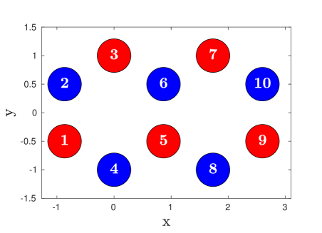
We first study the accuracy of the fTWA method on a small graphene-like few-body system. The system is composed of ten sites organised in two hexagonal cells, see Fig. 1, which makes it large enough to be interesting and small enough to compute numerical solutions with the Exact Diagonalisation method. The system is assumed to be electronically half-filled, which means that there are as many particles as there are sites. We also consider a system with equal amount of spin-up as spin-down electrons. For the initial condition, we choose the p𝑝p-particles Fock-space vector with the largest overlap to the ground state, where each site is filled with either a spin-up or spin-down particle, see Fig. 1. We motivate this choice further in Appendix B.2. The time evolution with the fTWA method has been computed with 105superscript10510^{5} trajectories, and until t=5𝑡5t=5, a choice that was made so that one can see when all methods considered here start to deviate from each other.
Refer to caption
Figure 1: (Color online) Illustration of one of the two dominating pure states of the ground state of the Hamiltonian (Eqn.1). Here we consider a 10 sites Fermi-Hubbard model with half filling. The geometry is composed of two perfect hexagons of equal side lengths. This state was used as initial condition for the quantum dynamics calculations. In blue, the spin-down sites, in red the spin-up sites. The second most dominating state is the spin symmetry of this one, i.e. a state where all electrons have flipped their spin (and blue and red colours have been interchanged in the figure).

IV.2 Evolution of occupations, first-order moments

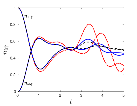
The first measure used to compare the methods is the time evolution of site occupations, niiσ(t)subscript𝑛𝑖𝑖𝜎𝑡n_{ii\sigma}(t). We show in Fig. 2 the occupation of spin-up particles on sites 111 and 555, respectively n11subscript𝑛11absentn_{11\uparrow} and n55subscript𝑛55absentn_{55\uparrow}. We see that the occupations computed with the Hartree-Fock method deviate from the exact solution (the ED method) at t1similar-to-or-equals𝑡1t\simeq 1 and that the occupations computed with fTWA starts to deviate later, at t3similar-to-or-equals𝑡3t\simeq 3. We stress that the only computational cost to achieve this improvement is that the calculation is repeated, in parallel, for the different trajectories.

Note that the computation times of both HF and fTWA methods scale quadratically with the system size, and the fTWA method is here correct for approximately three times longer. Here, using 105superscript10510^{5} trajectories in the fTWA method, the statistical error is negligible, hidden behind the width of the line. Hence, the deviation comes entirely from the truncation possible from the approximation of the initial density [18] in the formalism of the method, and is not due to statistical uncertainty. We also note an improvement on the long term dynamics. When t𝑡t\rightarrow\infty the occupation stabilizes at niiσ0.5similar-to-or-equalssubscript𝑛𝑖𝑖𝜎0.5n_{ii\sigma}\simeq 0.5 for all sites and spins (data not shown). This result is recovered by the fTWA method, but not by the HF one that oscillates uncontrollably.
Refer to caption
Figure 2: (Color online) Dynamics of site occupations for spin-up particles on sites 1 (n11subscript𝑛11n_{11}) and 5 (n55subscript𝑛55n_{55}). The solid (blue) curves show the fTWA dynamics, the dashed (black) ones show the exact diagonalisation dynamics, the dashed-dotted (red) ones the Hartree-Fock dynamics. For the occupation, the HF dynamic starts to deviate from the ED at t1similar-to-or-equals𝑡1t\simeq 1, while the fTWA dynamic starts to deviate from the ED solution at around t3similar-to-or-equals𝑡3t\simeq 3.

IV.3 Evolution of correlations, second-order moments

One advantage of phase-space methods, like fTWA, is their ability to give information on the dynamics of higher-order moments, like second-order correlation functions, even for large system. The correlation function between two sites i𝑖i, j𝑗j and spins σ1subscript𝜎1\sigma_{1}, σ2subscript𝜎2\sigma_{2}, here denoted giσ1,jσ2(2)subscriptsuperscript𝑔2𝑖subscript𝜎1𝑗subscript𝜎2g^{(2)}_{i\sigma_{1},j\sigma_{2}}, can be seen as the effect the presence of a spin-σ1subscript𝜎1\sigma_{1} particle on site i𝑖i has on the probability to have a spin-σ2subscript𝜎2\sigma_{2} particle on site j𝑗j. The explicit formulas are, in the Schrödinger picture for ED:

giσ1,jσ2(2)(t)=c^iσ1c^jσ2c^iσ1c^jσ2c^iσ1c^iσ1c^jσ2c^jσ2 ,subscriptsuperscript𝑔2𝑖subscript𝜎1𝑗subscript𝜎2𝑡delimited-⟨⟩superscriptsubscript^𝑐𝑖subscript𝜎1superscriptsubscript^𝑐𝑗subscript𝜎2subscript^𝑐𝑖subscript𝜎1subscript^𝑐𝑗subscript𝜎2delimited-⟨⟩superscriptsubscript^𝑐𝑖subscript𝜎1subscript^𝑐𝑖subscript𝜎1delimited-⟨⟩superscriptsubscript^𝑐𝑗subscript𝜎2subscript^𝑐𝑗subscript𝜎2 ,g^{(2)}_{i\sigma_{1},j\sigma_{2}}(t)=\frac{\langle\hat{c}_{i\sigma_{1}}^{\dagger}\hat{c}_{j\sigma_{2}}^{\dagger}\hat{c}_{i\sigma_{1}}\hat{c}_{j\sigma_{2}}\rangle}{\langle\hat{c}_{i\sigma_{1}}^{\dagger}\hat{c}_{i\sigma_{1}}\rangle\langle\hat{c}_{j\sigma_{2}}^{\dagger}\hat{c}_{j\sigma_{2}}\rangle}\text{ ,} (9)

and in the Heisenberg picture with the fTWA phase-space variables:

giσ1,jσ2(2)(t)=ρiiσρjjσ¯+(ρiiσ¯+ρjjσ¯)/2+1/4(ρiiσ¯+1/2)(ρjjσ¯+1/2)=(ρiiσ+1/2)(ρjjσ+1/2)¯(ρiiσ¯+1/2)(ρjjσ¯+1/2) .subscriptsuperscript𝑔2𝑖subscript𝜎1𝑗subscript𝜎2𝑡¯subscript𝜌𝑖𝑖𝜎subscript𝜌𝑗𝑗𝜎¯subscript𝜌𝑖𝑖𝜎¯subscript𝜌𝑗𝑗𝜎214¯subscript𝜌𝑖𝑖𝜎12¯subscript𝜌𝑗𝑗𝜎12¯subscript𝜌𝑖𝑖𝜎12subscript𝜌𝑗𝑗𝜎12¯subscript𝜌𝑖𝑖𝜎12¯subscript𝜌𝑗𝑗𝜎12 .\begin{split}g^{(2)}_{i\sigma_{1},j\sigma_{2}}(t)&=\frac{\overline{\rho_{ii\sigma}\rho_{jj\sigma}}+(\overline{\rho_{ii\sigma}}+\overline{\rho_{jj\sigma}})/2+1/4}{(\overline{\rho_{ii\sigma}}+1/2)(\overline{\rho_{jj\sigma}}+1/2)}\\ &=\frac{\overline{(\rho_{ii\sigma}+1/2)(\rho_{jj\sigma}+1/2)}}{(\overline{\rho_{ii\sigma}}+1/2)(\overline{\rho_{jj\sigma}}+1/2)}\text{ .}\end{split} (10)

For the mean-field Hartree-Fock approximation we use Wick’s theorem, see Eq. (14) in Appendix A.2.

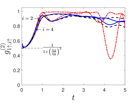
In Fig. 3, we plot the correlation between the spin-up particle on site 111 and the spin-up particles on the two neighboring sites, 222 and 444, see Fig. 1 for the geometry. The correlation computed with fTWA is essentially the same as that of ED, until approximately t2similar-to-or-equals𝑡2t\simeq 2 where it starts to deviate visibly. This happens earlier than for the occupation, shown in Fig. 2. At t0similar-to-or-equals𝑡0t\simeq 0, we observe that the correlation functions computed with fTWA does not tend precisely to its theoretical value, Eq. (31), of g1,2(2)=0.5subscriptsuperscript𝑔212absent0.5g^{(2)}_{1\uparrow,2\uparrow}=0.5. The quantitative difficulties fTWA has to compute correlations involving initial empty sites are known for bosons [21], the calculations made in Appendix C expose the same problem for the present Hamiltonian. In principle, these results can be improved by adding more trajectories or using projection methods.
Refer to caption
Figure 3: (Color online) Dynamics of correlation functions between neighbour sites, here g1,2(2)subscriptsuperscript𝑔212absentg^{(2)}_{1\uparrow,2\uparrow} and g1,4(2)subscriptsuperscript𝑔214absentg^{(2)}_{1\uparrow,4\uparrow}. The different curves represent the same methods and parameter values as described in Fig. 2.

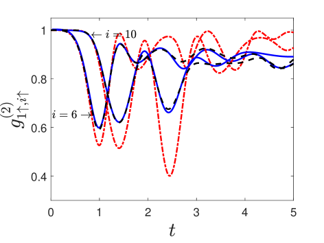
In Fig. 4, we plot the correlations between the spin-up particle on site 111 and the spin-up particles on distant sites, 666 and 101010, see again Fig. 1 for the geometry. We observe that the fTWA results starts to deviate from data obtained by ED, at a time between t2similar-to-or-equals𝑡2t\simeq 2 and t3similar-to-or-equals𝑡3t\simeq 3. We also observe in Fig. 4 that the time for a correlation to appear between two sites, i.e. when g(2)superscript𝑔2g^{(2)} deviate from unity, depends on the increasing distance between those two sites.
Refer to caption
Figure 4: (Color online) Dynamics of correlation functions between distant sites, here g1,6(2)subscriptsuperscript𝑔216absentg^{(2)}_{1\uparrow,6\uparrow} and g1,10(2)subscriptsuperscript𝑔2110absentg^{(2)}_{1\uparrow,10\uparrow}. The different curves represent the same methods and parameters values as described in Fig. 2.

In the case of different spins correlations, like e.g. gi,i(2)subscriptsuperscript𝑔2𝑖𝑖absentg^{(2)}_{i\uparrow,i\downarrow}, the second term in Eq. (14) is zero. As a consequence HF gives a constant, g(2)1superscript𝑔21g^{(2)}\equiv 1, and cannot be used for comparisons. However, fTWA gives accurate results for short times, as we have explored numerically in comparisons with ED for small systems.

IV.4 Large-time correlation functions

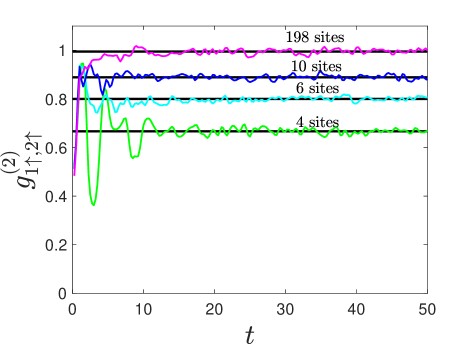
To investigate if the fTWA is also able to model the long term values of correlation functions, we computed the fTWA results of g1,2(2)subscriptsuperscript𝑔212absentg^{(2)}_{1\uparrow,2\uparrow} for systems of different size, n=4,6,10,198𝑛4610198n=4,6,10,198 sites, until t=50𝑡50t=50 (note that we did not plot other correlations for clarity, but they all tend to the same limits). The results are shown in Fig. 5, and we see that the correlation tends to the limits that correspond to equal probability for particles, see the explanation and examples in Appendix C.3. Correlations between all the other pairs of different sites and same-spin particles have the same limit. For n=4,6,10𝑛4610n=4,6,10, the fTWA results were compared with Exact Diagonalisation.
Refer to caption
Figure 5: (Color online) Long-time fTWA dynamics for correlations between spin-up particles on sites 111 and 222, g1,2(2)subscriptsuperscript𝑔212absentg^{(2)}_{1\uparrow,2\uparrow}, for systems of different size, n=4,6,10,198𝑛4610198n=4,6,10,198. The horizontal (black) lines represent the limit (t𝑡t\rightarrow\infty) values of correlation function gathered in table 1, we recover the values of formula (35) for all cases.

V fTWA on a large system

Refer to caption
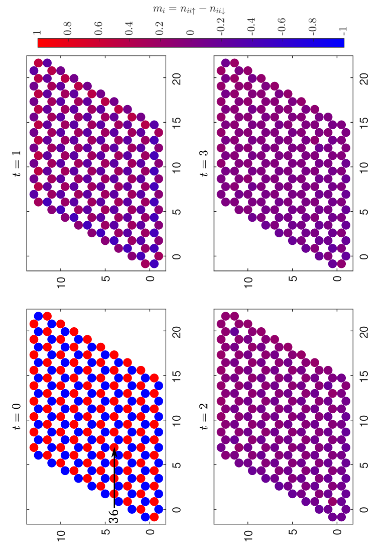
Figure 6: (Color online) Four different frames from the dynamics of the magnetic moment mi=niiniisubscript𝑚𝑖subscript𝑛𝑖subscript𝑖subscript𝑛𝑖subscript𝑖m_{i}=n_{ii_{\uparrow}}-n_{ii_{\downarrow}} for times t=0,1,2,3𝑡0123t=0,1,2,3. Sites in red have mi=1subscript𝑚𝑖1m_{i}=1, one spin-up particle, sites in blue have mi=1subscript𝑚𝑖1m_{i}=-1, one spin-down particle. Sites in purple have mi=0subscript𝑚𝑖0m_{i}=0. For larger times we see that the magnetic moments all stabilize to mi0similar-to-or-equalssubscript𝑚𝑖0m_{i}\simeq 0, when the system tends to nii=nii0.5subscript𝑛𝑖𝑖absentsubscript𝑛𝑖𝑖absentsimilar-to-or-equals0.5n_{ii\uparrow}=n_{ii\downarrow}\simeq 0.5.

Now that we have shown the ability of fTWA to efficiently model small Fermi-Hubbard systems, by a direct comparison to data from Exact Diagonalization, we study a substantially larger system, that is far out of reach for Exact Diagonalisation. We compute the dynamics of fermions described by the Hamiltonian of Eq. (1) on a graphene-like system with a honeycomb structure involving 198 sites, see the overall geometry in Fig. 6. In this figure the value of the magnetisation, mi=niiniisubscript𝑚𝑖subscript𝑛𝑖𝑖absentsubscript𝑛𝑖𝑖absentm_{i}=n_{ii\uparrow}-n_{ii\downarrow}, is shown for four time frames of the calculation. At t=0𝑡0t=0, the sites are filled with either a spin-up electron or a spin-down electron, represented by red and blue circles in Fig. 6, respectively. This represents a starting state similar to that considered in Fig. 1. For the subsequent times, the dynamics is such that the magnetisation at each site approaches zero (niinii0.5similar-to-or-equalssubscript𝑛𝑖𝑖absentsubscript𝑛𝑖𝑖absentsimilar-to-or-equals0.5n_{ii\uparrow}\simeq n_{ii\downarrow}\simeq 0.5), representing an equal occupation of spin-up and spin-down electrons. This is seen most clearly in Fig. 6 by the purple color of all sites at t=3𝑡3t=3. This result is consistent with experimental data of graphene at equilibrium conditions, that are known to reflect an equal occupation of spin-up and spin-down electrons [2].

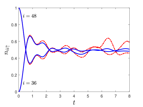
For a more accurate view of the dynamics, we have plotted in Fig. 7 the occupation of spin-up electrons on sites 363636 and 484848, n36subscript𝑛36absentn_{36\uparrow} and n48subscript𝑛48absentn_{48\uparrow}, i.e. from sites in the middle of the system. Within the short time of the simulation, effects of the boundary of the 198 atom cluster play little role, and the system appears infinite, as reflected in the visible symmetry between n36subscript𝑛36absentn_{36\uparrow} and n48subscript𝑛48absentn_{48\uparrow} in Fig. 7. This symmetry breaks at later times, around t4similar-to-or-equals𝑡4t\simeq 4. Note that the data in Fig. 7 contains results from HF and fTWA calculations and that for short simulation times (t3𝑡3t\leq 3) we find similar occupations for the two approaches, in contrast to the example in Fig. 2 that considered a smaller system. The size of the system gives the site interactions a more predominant role, which we expect makes HF and fTWA better approximations of the real particle dynamics, but clearly ED is out of reach for comparisons. Also, for longer simulation times, the HF method gives highly oscillatory results, as shown in Fig. 7, which is not the case for the fTWA method.
Refer to caption
Figure 7: (Color online) Dynamics of site occupation for spin-up particles on sites 363636 and 484848 for a 198 atom cluster. Data obtained by HF given by dashed red curves and fTWA full blue curves.

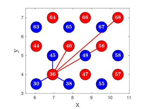
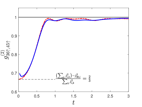
Similar to the smaller system, we also study for the 198 atom system the correlation functions between different sites. We picked a central site, numbered 363636, to be a representative one (see the arrow in the t=0𝑡0t=0 subplot in Fig. 6), and followed the correlation functions with one of its nearest neighbours as well as with further distant sites, see the geometry in Fig. 8. In Fig. 9 we show the correlation functions of spin-up particles with a near neighbour site, g36,45(2)(t)subscriptsuperscript𝑔23645absent𝑡g^{(2)}_{36\uparrow,45\uparrow}(t). The correlation for the three neighbours are initially very similar because of local symmetries in the large system, where edge effects of the cluster play a lesser role. We recognise the short-time limit (t0𝑡0t\rightarrow 0), where g(2)(0)=2/3superscript𝑔2023g^{(2)}(0)=2/3, because each site has three neighbours, see the derivation in Appendix C, and the deviation from the initial value that we saw in the smaller system, in Fig. 3. For longer time scales the data in Fig. 9 approach a value close to one, that only depends on the total number of sites, see Appendix C.3. Again one may note large oscillations with the HF method for longer times.

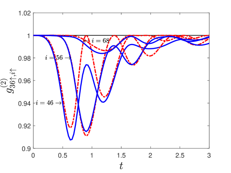
In Fig. 10 we have plotted the correlation functions between the site numbered 363636 and its neighbours at longer distance, see Fig. 8 for the geometry. Note that our choice of sites is such that they are initially filled with electrons of the same spin orientation, which means that at t=0𝑡0t=0 the correlation function is one. We can observe from Fig. 10 that the further away two sites are, the longer it takes before g(2)superscript𝑔2g^{(2)} starts to deviate from unity.

Refer to caption
Figure 8: (Color online) Zoom in on the 198-sites Fermi-Hubbard system, of Fig. 6, at t=0𝑡0t=0. The sites in red starts with a spin-up particle, e.g. n36(0)=1subscript𝑛36absent01n_{36\uparrow}(0)=1, and the blue ones starts with a spin-down particle, e.g. n48(0)=1subscript𝑛48absent01n_{48\downarrow}(0)=1. We will follow the correlation function of spin-up particles between the site 363636 and one of the three closest neighbours (blue lines) in Fig. 9. Then between site 363636 and three distant sites (red lines) in Fig. 10.
Refer to caption
Figure 9: (Color online) Dynamics of correlation functions between neighbour sites, here the site 363636 and a neighbour, site 454545. Data obtained by HF given by dashed red curves and fTWA full blue curves.
Refer to caption
Figure 10: (Color online) Dynamics of correlation functions between distant sites, here the site 363636 and sites 46,56,6846566846,56,68, see Fig. 8. Data obtained by HF given by dashed red curves and fTWA full blue curves.

VI Conclusion

In this work we have studied the quantum dynamics of the electronic structure of graphene-like systems, using an electronic Hamiltonian that allows for hopping and one-site Coulomb repulsion. The analysis is focused on the electron states close to the Fermi level, and are hence limited to pzsubscript𝑝𝑧p_{z} orbitals of spin-up or spin-down character centered on each site of a honeycomb lattice site. This allows to study the dynamics of an electronic Hamiltonian that includes the minimum interactions to represent a realistic system, i.e. the electron hopping and on-site Coulomb repulsion.

We have in this investigation compared three methods with which to solve the time evolution of the electronic system; the Exact Diagonalization technique, the Hartree-Fock (HF) approximation and the fermionic Truncated Wigner Approximation (fTWA). In comparing the three approaches for smaller graphene-like systems we conclude that fTWA reproduces the results of Exact Diagonalization, for significantly longer times compared to HF, and for this reason we have focused on fTWA for larger systems. Previous works of fTWA have focused on long-range interactions [12], but mean-field and phase-space representation methods have larger difficulties to model on-site interactions because of the more predominant role of quantum effects. Under those conditions, fTWA demonstrates a net improvement over mean-field methods. As shown here, the evolution of site occupations agrees well with exact results, for a period that is three times longer for fTWA compared to HF (see Fig. 2), and its long-time behaviour is also quantitatively recovered. The second-order correlation functions are also found to be well approximated, both on short-time dynamics (Figs. 3, 4) and long-time dynamics (Fig. 5). When comparing large and small systems, the results here are consistent with previous results; that smaller systems exhibit larger fluctuations in e.g. the correlation function, compared to larger ones.

The improvements of fTWA over mean-field methods come with an acceptable computational cost. A fTWA computation scales as O(n2)𝑂superscript𝑛2O(n^{2}) with the number of sites n𝑛n, similar to the HF computation. It needs however multiple repetitions of computations (trajectories) to average upon. This cost is manageable on a single computer for the systems studied here and embarrassingly parallelizable for larger systems.

Acknowledgments

We thank Joel Corney and Adam Sajna for valuable discussions. F. Rousse and M. Ögren  are supported by Carl Tryggers foundation and RR-ORU-2021/2022. O. Eriksson acknowledges support from the Swedish Research Council, the Knut and Alice Wallenberg Foundation, the European Research Council via Synergy Grant 854843 - FASTCORR, Energimyndigheten and eSSENCE.

References

  • Novoselov et al. [2004] K. S. Novoselov, A. K. Geim, S. V. Morozov, D.-e. Jiang, Y. Zhang, S. V. Dubonos, I. V. Grigorieva,  and A. A. Firsov, Science 306, 666 (2004).
  • Katsnelson [2007] M. I. Katsnelson, Materials Today 10, 20 (2007).
  • Geim and Novoselov [2010] A. K. Geim and K. S. Novoselov, in Nanoscience and technology: a collection of reviews from nature journals (World Scientific, 2010) pp. 11–19.
  • Wallace [1947] P. R. Wallace, Physical Review 71, 622 (1947).
  • McClure [1956] J. McClure, Physical Review 104, 666 (1956).
  • Neto et al. [2009] A. C. Neto, F. Guinea, N. M. Peres, K. S. Novoselov,  and A. K. Geim, Reviews of Modern Physics 81, 109 (2009).
  • Katsnelson et al. [2006] M. Katsnelson, K. Novoselov,  and A. Geim, Nature Physics 2, 620 (2006).
  • Katsnelson [2011] M. I. Katsnelson, in Graphene: carbon in two dimensions (Cambridge University Press, 2011) pp. 1–351.
  • Bolotin et al. [2008] K. I. Bolotin, K. J. Sikes, Z. Jiang, M. Klima, G. Fudenberg, J. Hone, P. Kim,  and H. L. Stormer, Solid State Communications 146, 351 (2008).
  • Panda et al. [2020] J. Panda, M. Ramu, O. Karis, T. Sarkar,  and M. V. Kamalakar, ACS nano 14, 12771 (2020).
  • Harrison [2012] W. A. Harrison, Electronic structure and the properties of solids: the physics of the chemical bond (Courier Corporation, 2012).
  • Sajna and Polkovnikov [2020] A. S. Sajna and A. Polkovnikov, Physical Review A 102, 033338 (2020).
  • Ma et al. [2011] T. Ma, F. Hu, Z. Huang,  and H.-Q. Lin, Computer Physics Communications 182, 52 (2011).
  • Joost et al. [2019] J.-P. Joost, N. Schlünzen,  and M. Bonitz, Physica Status Solidi (b) 256, 1800498 (2019).
  • Walls and Milburn [2007] D. F. Walls and G. J. Milburn, Quantum optics (Springer Science & Business Media, 2007).
  • Corney and Drummond [2006] J. F. Corney and P. D. Drummond, Physical Review B 73, 125112 (2006).
  • Ögren et al. [2010] M. Ögren, K. Kheruntsyan,  and J. Corney, EPL (Europhysics Letters) 92, 36003 (2010).
  • Davidson et al. [2017] S. M. Davidson, D. Sels,  and A. Polkovnikov, Annals of Physics 384, 128 (2017).
  • Sidje [1998] R. B. Sidje, ACM Transactions on Mathematical Software (TOMS) 24, 130 (1998).
  • Rahav and Mukamel [2009] S. Rahav and S. Mukamel, Physical Review B 79, 165103 (2009).
  • Sinatra et al. [2002] A. Sinatra, C. Lobo,  and Y. Castin, Journal of Physics B: Atomic, Molecular and Optical Physics 35, 3599 (2002).
  • Wick [1950] G.-C. Wick, Physical Review 80, 268 (1950).
  • Davidson and Polkovnikov [2015] S. M. Davidson and A. Polkovnikov, Physical Review Letters 114, 045701 (2015).

Appendix

Appendix A Derivation of differential equations for the quantum dynamics

In this appendix, we outline some of the details needed for the computations described in the main text. In the following, the indices written as Greek letters are pairs of position and spin, α=(a,σa)𝛼𝑎subscript𝜎𝑎\alpha=(a,\sigma_{a}).

A.1 Heisenberg equation of motion

In the Heisenberg picture, the operators are time dependent and evolve according to the differential equation:

ddtA^=i[H^,A^].𝑑𝑑𝑡^𝐴𝑖^𝐻^𝐴.\frac{d}{dt}\hat{A}=i\left[\hat{H},\hat{A}\right]\text{.} (11)

Hence for a Fermi-Hubbard Hamiltonian described in Eq. (1) with symmetric electron-electron interactions uαβ=uβαsubscript𝑢𝛼𝛽subscript𝑢𝛽𝛼u_{\alpha\beta}=u_{\beta\alpha}, the differential equation of a bilinear operators like c^αc^βsuperscriptsubscript^𝑐𝛼subscript^𝑐𝛽\hat{c}_{\alpha}^{\dagger}\hat{c}_{\beta} is

tc^αc^β=iμ((jβμc^αc^μjμαc^μc^β)+(uμαuβμ)c^αc^μc^μc^β).𝑡subscriptsuperscript^𝑐𝛼subscript^𝑐𝛽𝑖subscript𝜇subscript𝑗𝛽𝜇superscriptsubscript^𝑐𝛼subscript^𝑐𝜇subscript𝑗𝜇𝛼superscriptsubscript^𝑐𝜇subscript^𝑐𝛽subscript𝑢𝜇𝛼subscript𝑢𝛽𝜇subscriptsuperscript^𝑐𝛼superscriptsubscript^𝑐𝜇subscript^𝑐𝜇subscript^𝑐𝛽.\begin{split}\frac{\partial}{\partial t}\hat{c}^{\dagger}_{\alpha}\hat{c}_{\beta}&=i\sum_{\mu}\bigg{(}(j_{\beta\mu}\hat{c}_{\alpha}^{\dagger}\hat{c}_{\mu}-j_{\mu\alpha}\hat{c}_{\mu}^{\dagger}\hat{c}_{\beta})\\ &+(u_{\mu\alpha}-u_{\beta\mu})\hat{c}^{\dagger}_{\alpha}\hat{c}_{\mu}^{\dagger}\hat{c}_{\mu}\hat{c}_{\beta}\bigg{)}\text{.}\end{split} (12)

This differential equation for the number operators cannot be solved directly in practice, and we need to invoke approximations to obtain differential equations for complex numbers.

A.2 Mean-field approximation

In the Hartree-Fock approximation, the many-body wave-function is described as a product of one-body wave-functions, hence the system is always a single Slater determinant. That allows us to reduce the description of the electrons to a single-particle density matrix with

nαβc^αc^β.subscript𝑛𝛼𝛽delimited-⟨⟩superscriptsubscript^𝑐𝛼subscript^𝑐𝛽.\begin{split}n_{\alpha\beta}\equiv\langle\hat{c}_{\alpha}^{\dagger}\hat{c}_{\beta}\rangle\text{.}\end{split} (13)

For the two-body operators, we use Wick’s theorem [20, 22]:

c^αc^βc^γc^δnαδnβγnαγnβδ.delimited-⟨⟩superscriptsubscript^𝑐𝛼superscriptsubscript^𝑐𝛽subscript^𝑐𝛾subscript^𝑐𝛿subscript𝑛𝛼𝛿subscript𝑛𝛽𝛾subscript𝑛𝛼𝛾subscript𝑛𝛽𝛿.\begin{split}\langle\hat{c}_{\alpha}^{\dagger}\hat{c}_{\beta}^{\dagger}\hat{c}_{\gamma}\hat{c}_{\delta}\rangle\equiv n_{\alpha\delta}n_{\beta\gamma}-n_{\alpha\gamma}n_{\beta\delta}\text{.}\end{split} (14)

Which gives the differential equation for the single-particle density matrix:

tnαβ=iμ((jβμnαμjμαnμβ)+(uμαuβμ)(nαβnμμnαμnμβ)).𝑡subscript𝑛𝛼𝛽𝑖subscript𝜇subscript𝑗𝛽𝜇subscript𝑛𝛼𝜇subscript𝑗𝜇𝛼subscript𝑛𝜇𝛽subscript𝑢𝜇𝛼subscript𝑢𝛽𝜇subscript𝑛𝛼𝛽subscript𝑛𝜇𝜇subscript𝑛𝛼𝜇subscript𝑛𝜇𝛽.\begin{split}\frac{\partial}{\partial t}n_{\alpha\beta}&=i\sum_{\mu}\bigg{(}(j_{\beta\mu}n_{\alpha\mu}-j_{\mu\alpha}n_{\mu\beta})\\ &+(u_{\mu\alpha}-u_{\beta\mu})(n_{\alpha\beta}n_{\mu\mu}-n_{\alpha\mu}n_{\mu\beta})\bigg{)}\text{.}\end{split} (15)

In the Hamiltonian (1), no term allows the particle’s spin to flip, (jαβ=jabδσaσbsubscript𝑗𝛼𝛽subscript𝑗𝑎𝑏subscript𝛿subscript𝜎𝑎subscript𝜎𝑏j_{\alpha\beta}=j_{ab}\delta_{\sigma_{a}\sigma_{b}}) so variables representing spin-flip are always null and are neglected. Moreover, the electron-electron interaction is only between opposite-spin particles, uαβ=uabδσaσb¯subscript𝑢𝛼𝛽subscript𝑢𝑎𝑏subscript𝛿subscript𝜎𝑎¯subscript𝜎𝑏u_{\alpha\beta}=u_{ab}\delta_{\sigma_{a}\bar{\sigma_{b}}}. We denote nijσ=niσ,jσsubscript𝑛𝑖𝑗𝜎subscript𝑛𝑖𝜎𝑗𝜎n_{ij\sigma}=n_{i\sigma,j\sigma}, and Eq. (15) then becomes

tnijσ=il(jjlnilσjlinljσ+(uilulj)nllσ¯nijσ).𝑡subscript𝑛𝑖𝑗𝜎𝑖subscript𝑙subscript𝑗𝑗𝑙subscript𝑛𝑖𝑙𝜎subscript𝑗𝑙𝑖subscript𝑛𝑙𝑗𝜎subscript𝑢𝑖𝑙subscript𝑢𝑙𝑗subscript𝑛𝑙𝑙¯𝜎subscript𝑛𝑖𝑗𝜎.\begin{split}\frac{\partial}{\partial t}n_{ij\sigma}&=i\sum_{l}\big{(}j_{jl}n_{il\sigma}-j_{li}n_{lj\sigma}+(u_{il}-u_{lj})n_{ll\bar{\sigma}}n_{ij\sigma}\big{)}\text{.}\\ \end{split} (16)

These are the Hartree-Fock differential equations, as presented in Ref. [20].

A.3 Fermionic Truncated Wigner approximation

The fTWA is one of the phase-space representation methods, where we use a distribution to describe the electrons density matrix and map operators averages to the distribution’s moments. For the fTWA in systems with constant number of particles, we can choose the symmetrically ordered one-body operator E^βαsubscriptsuperscript^𝐸𝛼𝛽\hat{E}^{\alpha}_{\beta} we defined in Eq. (4) and map it to the phase-space variables ραβsubscript𝜌𝛼𝛽\rho_{\alpha\beta}. First-order and second-order moments of the phase-space variable distribution are linked respectively to one-body and two-body operators:

ραβ¯=W(ρ)ραβ𝑑ρ=E^αβ,ραβρμν¯=W(ρ)ραβρμν𝑑ρ=12E^βαE^μν+E^μνE^βα.¯subscript𝜌𝛼𝛽𝑊𝜌subscript𝜌𝛼𝛽differential-d𝜌delimited-⟨⟩superscriptsubscript^𝐸𝛼𝛽,¯superscriptsubscript𝜌𝛼𝛽subscript𝜌𝜇𝜈𝑊𝜌subscriptsuperscript𝜌𝛼𝛽subscript𝜌𝜇𝜈differential-d𝜌12delimited-⟨⟩superscriptsubscript^𝐸𝛽𝛼superscriptsubscript^𝐸𝜇𝜈superscriptsubscript^𝐸𝜇𝜈superscriptsubscript^𝐸𝛽𝛼.\begin{split}\overline{\rho_{\alpha\beta}}=\int W(\rho)\rho_{\alpha\beta}d\rho&=\langle\hat{E}_{\alpha}^{\beta}\rangle\text{,}\\ \overline{\rho_{\alpha\beta}^{*}\rho_{\mu\nu}}=\int W(\rho)\rho^{*}_{\alpha\beta}\rho_{\mu\nu}d\rho&=\frac{1}{2}\langle\hat{E}_{\beta}^{\alpha}\hat{E}_{\mu}^{\nu}+\hat{E}_{\mu}^{\nu}\hat{E}_{\beta}^{\alpha}\rangle\text{.}\\ \end{split} (17)

From those equations we can find the links between first- and second-order stochastic averages of phase-space variables and quantum operators in e.g. Eq. (5).

To obtain the equations of motion of the phase-space distribution, we follow the work of Polkovnikov [23, 18]. Here a Jordan-Schwinger mapping from the fermionic operators E^^𝐸\hat{E} to pair-bosonic operators was introduced, then the bosonic Truncated Wigner Approximation formalism can be applied. It was shown that the equation of motion for the phase-space variables ραβsubscript𝜌𝛼𝛽\rho_{\alpha\beta} are determined by the Poisson brackets

tραβ=i{ραβ,HW}=iγδf(α,β,μ,ν,γ,δ)HWρμνργδ,𝑡subscript𝜌𝛼𝛽𝑖subscript𝜌𝛼𝛽subscript𝐻𝑊𝑖subscript𝛾𝛿𝑓𝛼𝛽𝜇𝜈𝛾𝛿subscript𝐻𝑊subscript𝜌𝜇𝜈subscript𝜌𝛾𝛿,\begin{split}\frac{\partial}{\partial t}\rho_{\alpha\beta}&=i\{\rho_{\alpha\beta},H_{W}\}=i\sum_{\gamma\delta}f(\alpha,\beta,\mu,\nu,\gamma,\delta)\frac{\partial H_{W}}{\partial\rho_{\mu\nu}}\rho_{\gamma\delta}\text{,}\end{split} (18)

with f𝑓f being the structure constants of the bilinear operators;

[E^βα,E^νμ]=γδf(α,β,μ,ν,γ,δ)E^δγ=δμβE^ναδανE^βμ.superscriptsubscript^𝐸𝛽𝛼superscriptsubscript^𝐸𝜈𝜇subscript𝛾𝛿𝑓𝛼𝛽𝜇𝜈𝛾𝛿superscriptsubscript^𝐸𝛿𝛾subscript𝛿𝜇𝛽superscriptsubscript^𝐸𝜈𝛼subscript𝛿𝛼𝜈superscriptsubscript^𝐸𝛽𝜇.\begin{split}[\hat{E}_{\beta}^{\alpha},\hat{E}_{\nu}^{\mu}]&=\sum_{\gamma\delta}f(\alpha,\beta,\mu,\nu,\gamma,\delta)\hat{E}_{\delta}^{\gamma}\\ &=\delta_{\mu\beta}\hat{E}_{\nu}^{\alpha}-\delta_{\alpha\nu}\hat{E}_{\beta}^{\mu}\text{.}\end{split} (19)

In the expression above, HWsubscript𝐻𝑊H_{W} is the Hamiltonian in the ραβsubscript𝜌𝛼𝛽\rho_{\alpha\beta} variables:

HW=i,j,σjijρijσ+ijuij(ρii+12)(ρjj+12),subscript𝐻𝑊subscript𝑖𝑗𝜎subscript𝑗𝑖𝑗subscript𝜌𝑖𝑗𝜎subscript𝑖𝑗subscript𝑢𝑖𝑗subscript𝜌𝑖𝑖absent12subscript𝜌𝑗𝑗absent12,H_{W}=-\sum_{i,j,\sigma}j_{ij}\rho_{ij\sigma}+\sum_{i\geq j}u_{ij}\left(\rho_{ii\uparrow}+\frac{1}{2}\ \right)\left(\rho_{jj\downarrow}+\frac{1}{2}\ \right)\text{,} (20)

which gives us the differential equation (6).

We may not be able to reproduce all exact initial Wigner function with all high-order moments, but within the accuracy of the truncation, the two first moments are sufficient. So we approximate W(ρ,0)𝑊𝜌0W(\rho,0) with a gaussian distribution having the same first- and second-order moments (mean and covariance). From the relations (17) we compute the covariance between phase-space variables:

cov(ραβ,ρμν)=ραβρμν¯ραβ¯ρμν¯=12c^βc^αc^μc^ν+c^μc^νc^βc^αc^βc^αc^μc^ν=12(n~μαnβν+n~βνnμα),covsubscriptsuperscript𝜌𝛼𝛽subscript𝜌𝜇𝜈¯subscriptsuperscript𝜌𝛼𝛽subscript𝜌𝜇𝜈¯subscriptsuperscript𝜌𝛼𝛽¯subscript𝜌𝜇𝜈12delimited-⟨⟩subscriptsuperscript^𝑐𝛽subscript^𝑐𝛼subscriptsuperscript^𝑐𝜇subscript^𝑐𝜈subscriptsuperscript^𝑐𝜇subscript^𝑐𝜈subscriptsuperscript^𝑐𝛽subscript^𝑐𝛼delimited-⟨⟩subscriptsuperscript^𝑐𝛽subscript^𝑐𝛼delimited-⟨⟩subscriptsuperscript^𝑐𝜇subscript^𝑐𝜈12subscript~𝑛𝜇𝛼subscript𝑛𝛽𝜈subscript~𝑛𝛽𝜈subscript𝑛𝜇𝛼,\begin{split}\text{cov}(\rho^{*}_{\alpha\beta},\rho_{\mu\nu})&=\overline{\rho^{*}_{\alpha\beta}\rho_{\mu\nu}}-\overline{\rho^{*}_{\alpha\beta}}\overline{\rho_{\mu\nu}}\\ &=\frac{1}{2}\langle\hat{c}^{\dagger}_{\beta}\hat{c}_{\alpha}\hat{c}^{\dagger}_{\mu}\hat{c}_{\nu}+\hat{c}^{\dagger}_{\mu}\hat{c}_{\nu}\hat{c}^{\dagger}_{\beta}\hat{c}_{\alpha}\rangle-\langle\hat{c}^{\dagger}_{\beta}\hat{c}_{\alpha}\rangle\langle\hat{c}^{\dagger}_{\mu}\hat{c}_{\nu}\rangle\\ &=\frac{1}{2}(\tilde{n}_{\mu\alpha}n_{\beta\nu}+\tilde{n}_{\beta\nu}n_{\mu\alpha})\text{,}\end{split} (21)

with n~αβ=δαβnαβsubscript~𝑛𝛼𝛽subscript𝛿𝛼𝛽subscript𝑛𝛼𝛽\tilde{n}_{\alpha\beta}=\delta_{\alpha\beta}-n_{\alpha\beta}. In a diagonalising basis, nαβ=0subscript𝑛𝛼𝛽0n_{\alpha\beta}=0 if αβ𝛼𝛽\alpha\neq\beta, so the only non zero terms are

cov(ραβ,ραβ)=12(n~ααnββ+n~ββnαα)=12(nββ+nαα2nββnαα).covsubscriptsuperscript𝜌𝛼𝛽subscript𝜌𝛼𝛽12subscript~𝑛𝛼𝛼subscript𝑛𝛽𝛽subscript~𝑛𝛽𝛽subscript𝑛𝛼𝛼12subscript𝑛𝛽𝛽subscript𝑛𝛼𝛼2subscript𝑛𝛽𝛽subscript𝑛𝛼𝛼.\begin{split}\text{cov}(\rho^{*}_{\alpha\beta},\rho_{\alpha\beta})&=\frac{1}{2}(\tilde{n}_{\alpha\alpha}n_{\beta\beta}+\tilde{n}_{\beta\beta}n_{\alpha\alpha})\\ &=\frac{1}{2}(n_{\beta\beta}+n_{\alpha\alpha}-2n_{\beta\beta}n_{\alpha\alpha})\text{.}\\ \end{split} (22)

Hence we arrive at Eq. (7) for the random starting point of trajectories.

Appendix B Exact Diagonalisation

B.1 Exact Diagonalisation basis

In Eq. (8) describing the wave-function evolution, |Ψ(t)ketΨ𝑡\ket{\Psi(t)} is written in a finite basis |ψiketsubscript𝜓𝑖\ket{\psi_{i}} of Slater determinants of p𝑝p particles:

|Ψ(t)ketΨ𝑡\displaystyle\ket{\Psi(t)} =ibi(t)|ψi ,absentsubscript𝑖subscript𝑏𝑖𝑡ketsubscript𝜓𝑖 ,\displaystyle=\sum_{i}b_{i}(t)\ket{\psi_{i}}\text{ , } (23)
|ψiketsubscript𝜓𝑖\displaystyle\ket{\psi_{i}} =c^α1,ic^α2,ic^αp,i|0 .absentsuperscriptsubscript^𝑐subscript𝛼1𝑖superscriptsubscript^𝑐subscript𝛼2𝑖superscriptsubscript^𝑐subscript𝛼𝑝𝑖ket0 .\displaystyle=\hat{c}_{\alpha_{1,i}}^{\dagger}\hat{c}_{\alpha_{2,i}}^{\dagger}...\hat{c}_{\alpha_{p,i}}^{\dagger}\ket{0}\text{ .} (24)

If our system has n𝑛n sites and p𝑝p particles, we need Cnp=n!p!(np)!subscriptsuperscript𝐶𝑝𝑛𝑛𝑝𝑛𝑝C^{p}_{n}=\frac{n!}{p!(n-p)!} basis functions, which explains the impossibility to model systems of more than 202020 sites on a standard computer.

B.2 Analysis of the ground state

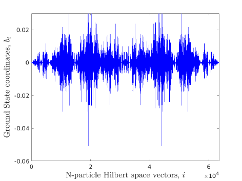
As initial condition for the dynamics, we are looking for a position eigenstate that has the largest overlap with the ground state of the Hamiltonian (1). In Fig. 11, we have plotted a representation of the ground state |Ψgs=ibi|ψiketsubscriptΨ𝑔𝑠subscript𝑖subscript𝑏𝑖ketsubscript𝜓𝑖\ket{\Psi_{gs}}=\sum_{i}b_{i}\ket{\psi_{i}}. On the x-axis are the indices of the N-particle Hilbert basis vectors and on the y-axis are the coordinates of the ground state in this basis, bisubscript𝑏𝑖b_{i}. We find two vectors that stand out with bi0.05similar-to-or-equalssubscript𝑏𝑖0.05b_{i}\simeq-0.05, the first one is the initial condition we have chosen, see Fig. 1, the other one is its spin symmetric state.
Refer to caption
Figure 11: Ground state representation of the Fermi-Hubbard system with 10 sites, 5 spin-up and 5 spin-down particles. If |Ψgs=ibi|ψiketsubscriptΨ𝑔𝑠subscript𝑖subscript𝑏𝑖ketsubscript𝜓𝑖\ket{\Psi_{gs}}=\sum_{i}b_{i}\ket{\psi_{i}}, the x-axis represents the N-particle Hilbert space vector indices i𝑖i in a given order, and the y-axis represents the value of the coefficients of those basis vectors, bisubscript𝑏𝑖b_{i}. We have chosen the first basis vector with the larger absolute coordinate, bi0.05similar-to-or-equalssubscript𝑏𝑖0.05b_{i}\simeq-0.05, as initial condition for the dynamics reported in the main text.

When we let the dynamics evolve, we have found that the density on all sites tends to 0.50.50.5 for large times. The corresponding t𝑡t\rightarrow\infty wave-function is a broad distribution of all N-particle Hilbert space vectors, |Ψ(t)ibi()|ψiketΨ𝑡subscript𝑖subscript𝑏𝑖ketsubscript𝜓𝑖\ket{\Psi(t)}\rightarrow\sum_{i}b_{i}(\infty)\ket{\psi_{i}} with |bi()|21/Nsimilar-to-or-equalssuperscriptsubscript𝑏𝑖21𝑁|b_{i}(\infty)|^{2}\simeq 1/N.

Appendix C Derivation of asymptotes of correlation functions

C.1 Short-time limit of correlations

We here show that the fTWA equations and the initial conditions leads to the correct values of the correlation functions for neighbour sites in the short-time limit. Lets compute g1,2(2)(0)subscriptsuperscript𝑔212absent0g^{(2)}_{1\uparrow,2\uparrow}(0), i.e. the correlation of spin-up particles between site 111 and site 222 in a system like in Fig. 1 when t0𝑡0t\rightarrow 0. From Eq. (10) we have,

g1,2(2)=(ρ11+1/2)(ρ22+1/2)ρ11+1/2ρ22+1/2 .subscriptsuperscript𝑔212absentdelimited-⟨⟩subscript𝜌11absent12subscript𝜌22absent12delimited-⟨⟩subscript𝜌11absent12delimited-⟨⟩subscript𝜌22absent12 .g^{(2)}_{1\uparrow,2\uparrow}=\frac{\langle(\rho_{11\uparrow}+1/2)(\rho_{22\uparrow}+1/2)\rangle}{\langle\rho_{11\uparrow}+1/2\rangle\langle\rho_{22\uparrow}+1/2\rangle}\text{ .} (25)

In this appendix, the brackets delimited-⟨⟩\langle...\rangle denote stochastic average. From the initial conditions, we can first derive the first order approximation of the off-diagonal terms ρ12subscript𝜌12absent\rho_{12\uparrow}, ρ21subscript𝜌21absent\rho_{21\uparrow}, ρ23subscript𝜌23absent\rho_{23\uparrow} and ρ32subscript𝜌32absent\rho_{32\uparrow}:

tρ12𝑡subscript𝜌12absent\displaystyle\frac{\partial}{\partial t}\rho_{12\uparrow} =ik(j2kρ1kjk1ρk2)+iuρ12(ρ11ρ22)absent𝑖subscript𝑘subscript𝑗2𝑘subscript𝜌1𝑘absentsubscript𝑗𝑘1subscript𝜌𝑘2absent𝑖𝑢subscript𝜌12absentsubscript𝜌11absentsubscript𝜌22absent\displaystyle=i\sum_{k}(j_{2k}\rho_{1k\uparrow}-j_{k1}\rho_{k2\uparrow})+iu\rho_{12\uparrow}(\rho_{11\downarrow}-\rho_{22\downarrow})
=i(j12(ρ11ρ22)+j32ρ13j14ρ42)absent𝑖subscript𝑗12subscript𝜌11absentsubscript𝜌22absentsubscript𝑗32subscript𝜌13absentsubscript𝑗14subscript𝜌42absent\displaystyle=i\big{(}j_{12}(\rho_{11\uparrow}-\rho_{22\uparrow})+j_{32}\rho_{13\uparrow}-j_{14}\rho_{42\uparrow}\big{)}
+iuρ12(ρ11ρ22) .𝑖𝑢subscript𝜌12absentsubscript𝜌11absentsubscript𝜌22absent .\displaystyle\leavevmode\nobreak\ \leavevmode\nobreak\ +iu\rho_{12\uparrow}(\rho_{11\downarrow}-\rho_{22\downarrow})\text{ .}

Now, since at t=0𝑡0t=0, n11(0)=n33(0)=1subscript𝑛11absent0subscript𝑛33absent01n_{11\uparrow}(0)=n_{33\uparrow}(0)=1, n22(0)=n44(0)=0subscript𝑛22absent0subscript𝑛44absent00n_{22\uparrow}(0)=n_{44\uparrow}(0)=0, and ρ13(0)=ρ42(0)=0subscript𝜌13absent0subscript𝜌42absent00\rho_{13\uparrow}(0)=\rho_{42\uparrow}(0)=0, see the initial conditions (7) for the system in Fig. 1, we have:

ddtρ12(0)𝑑𝑑𝑡subscript𝜌12absent0\displaystyle\frac{d}{dt}\rho_{12\uparrow}(0) =iuξ122+ij12.absent𝑖𝑢subscript𝜉12absent2𝑖subscript𝑗12\displaystyle=-iu\frac{\xi_{12\uparrow}}{\sqrt{2}}+ij_{12}.

Hence, for the short-time dynamics, i.e. for t=ϵ1𝑡italic-ϵmuch-less-than1t=\epsilon\ll 1,

ρ12(ϵ)subscript𝜌12absentitalic-ϵ\displaystyle\rho_{12\uparrow}(\epsilon) =ξ122+0ϵddtρ12𝑑tabsentsubscript𝜉12absent2superscriptsubscript0italic-ϵ𝑑𝑑𝑡subscript𝜌12absentdifferential-d𝑡\displaystyle=\frac{\xi_{12\uparrow}}{\sqrt{2}}+\int_{0}^{\epsilon}\frac{d}{dt}\rho_{12\uparrow}dt
=ξ122+0ϵ(ddtρ12|t=0+O(t))𝑑tabsentsubscript𝜉12absent2superscriptsubscript0italic-ϵevaluated-at𝑑𝑑𝑡subscript𝜌12absent𝑡0𝑂𝑡differential-d𝑡\displaystyle=\frac{\xi_{12\uparrow}}{\sqrt{2}}+\int_{0}^{\epsilon}\left(\frac{d}{dt}\rho_{12\uparrow}\bigg{|}_{t=0}+O(t)\right)dt
=ξ122+ij12ϵiuξ122ϵ+O(ϵ2) .absentsubscript𝜉12absent2𝑖subscript𝑗12italic-ϵ𝑖𝑢subscript𝜉12absent2italic-ϵ𝑂superscriptitalic-ϵ2 .\displaystyle=\frac{\xi_{12\uparrow}}{\sqrt{2}}+ij_{12}\epsilon-iu\frac{\xi_{12\uparrow}}{\sqrt{2}}\epsilon+O(\epsilon^{2})\text{ .}

In the same way, we obtain:

ρ21(ϵ)=ξ212ij12ϵ+iuξ212ϵ+O(ϵ2),ρ23(ϵ)=ξ232ij32ϵ+iuξ232ϵ+O(ϵ2),ρ32(ϵ)=ξ322+ij32ϵiuξ322ϵ+O(ϵ2).formulae-sequencesubscript𝜌21absentitalic-ϵsubscript𝜉21absent2𝑖subscript𝑗12italic-ϵ𝑖𝑢subscript𝜉21absent2italic-ϵ𝑂superscriptitalic-ϵ2formulae-sequencesubscript𝜌23absentitalic-ϵsubscript𝜉23absent2𝑖subscript𝑗32italic-ϵ𝑖𝑢subscript𝜉23absent2italic-ϵ𝑂superscriptitalic-ϵ2subscript𝜌32absentitalic-ϵsubscript𝜉32absent2𝑖subscript𝑗32italic-ϵ𝑖𝑢subscript𝜉32absent2italic-ϵ𝑂superscriptitalic-ϵ2\begin{split}\rho_{21\uparrow}(\epsilon)&=\frac{\xi_{21\uparrow}}{\sqrt{2}}-ij_{12}\epsilon+iu\frac{\xi_{21\uparrow}}{\sqrt{2}}\epsilon+O(\epsilon^{2}),\\ \rho_{23\uparrow}(\epsilon)&=\frac{\xi_{23\uparrow}}{\sqrt{2}}-ij_{32}\epsilon+iu\frac{\xi_{23\uparrow}}{\sqrt{2}}\epsilon+O(\epsilon^{2}),\\ \rho_{32\uparrow}(\epsilon)&=\frac{\xi_{32\uparrow}}{\sqrt{2}}+ij_{32}\epsilon-iu\frac{\xi_{32\uparrow}}{\sqrt{2}}\epsilon+O(\epsilon^{2}).\end{split} (26)

With these expressions, we can derive approximations of ρ11subscript𝜌11absent\rho_{11\uparrow} and ρ22subscript𝜌22absent\rho_{22\uparrow} with a second-order accuracy in t𝑡t. For arbitrary t𝑡t, we have

ddtρ11𝑑𝑑𝑡subscript𝜌11absent\displaystyle\frac{d}{dt}\rho_{11\uparrow} =ik(j2kρ1kjk1ρk1)+iuρ11(ρ11ρ11)absent𝑖subscript𝑘subscript𝑗2𝑘subscript𝜌1𝑘absentsubscript𝑗𝑘1subscript𝜌𝑘1absent𝑖𝑢subscript𝜌11absentsubscript𝜌11absentsubscript𝜌11absent\displaystyle=i\sum_{k}(j_{2k}\rho_{1k\uparrow}-j_{k1}\rho_{k1\uparrow})+iu\rho_{11\uparrow}(\rho_{11\downarrow}-\rho_{11\downarrow})
=ij12(ρ12ρ21)+ij14(ρ14ρ41)) .\displaystyle=ij_{12}(\rho_{12\uparrow}-\rho_{21\uparrow})+ij_{14}(\rho_{14\uparrow}-\rho_{41\uparrow}))\text{ .}

Hence, for t=ϵ1𝑡italic-ϵmuch-less-than1t=\epsilon\ll 1, we can insert the off-diagonal terms of Eq. (26):

iddtρ11(ϵ)𝑖𝑑𝑑𝑡subscript𝜌11absentitalic-ϵ\displaystyle i\frac{d}{dt}\rho_{11\uparrow}(\epsilon)
=\displaystyle= j12(ξ122ij12ϵ+iuξ122ϵξ122ij12ϵ+iuξ122ϵ)subscript𝑗12subscriptsuperscript𝜉12absent2𝑖subscript𝑗12italic-ϵ𝑖𝑢subscriptsuperscript𝜉12absent2italic-ϵsubscript𝜉12absent2𝑖subscript𝑗12italic-ϵ𝑖𝑢subscript𝜉12absent2italic-ϵ\displaystyle j_{12}\left(\frac{\xi^{*}_{12\uparrow}}{\sqrt{2}}-ij_{12}\epsilon+iu\frac{\xi^{*}_{12\uparrow}}{\sqrt{2}}\epsilon-\frac{\xi_{12\uparrow}}{\sqrt{2}}-ij_{12}\epsilon+iu\frac{\xi_{12\uparrow}}{\sqrt{2}}\epsilon\right)
+j14(ξ142ij14ϵ+iuξ142ϵξ142ij14ϵ+iuξ142ϵ)subscript𝑗14subscriptsuperscript𝜉14absent2𝑖subscript𝑗14italic-ϵ𝑖𝑢subscriptsuperscript𝜉14absent2italic-ϵsubscript𝜉14absent2𝑖subscript𝑗14italic-ϵ𝑖𝑢subscript𝜉14absent2italic-ϵ\displaystyle+j_{14}\left(\frac{\xi^{*}_{14\uparrow}}{\sqrt{2}}-ij_{14}\epsilon+iu\frac{\xi^{*}_{14\uparrow}}{\sqrt{2}}\epsilon-\frac{\xi_{14\uparrow}}{\sqrt{2}}-ij_{14}\epsilon+iu\frac{\xi_{14\uparrow}}{\sqrt{2}}\epsilon\right)
+O(ϵ2)𝑂superscriptitalic-ϵ2\displaystyle+O(\epsilon^{2})
=\displaystyle= ij12ξ12ξ1222j122ϵ+uj12ξ12+ξ122ϵ𝑖subscript𝑗12subscript𝜉12absentsubscriptsuperscript𝜉12absent22superscriptsubscript𝑗122italic-ϵ𝑢subscript𝑗12subscript𝜉12absentsubscriptsuperscript𝜉12absent2italic-ϵ\displaystyle ij_{12}\frac{\xi_{12\uparrow}-\xi^{*}_{12\uparrow}}{\sqrt{2}}-2j_{12}^{2}\epsilon+uj_{12}\frac{\xi_{12\uparrow}+\xi^{*}_{12\uparrow}}{\sqrt{2}}\epsilon
+ij14ξ14ξ1422j142ϵ+uj14ξ14+ξ142ϵ+O(ϵ2)𝑖subscript𝑗14subscript𝜉14absentsubscriptsuperscript𝜉14absent22superscriptsubscript𝑗142italic-ϵ𝑢subscript𝑗14subscript𝜉14absentsubscriptsuperscript𝜉14absent2italic-ϵ𝑂superscriptitalic-ϵ2\displaystyle+ij_{14}\frac{\xi_{14\uparrow}-\xi^{*}_{14\uparrow}}{\sqrt{2}}-2j_{14}^{2}\epsilon+uj_{14}\frac{\xi_{14\uparrow}+\xi^{*}_{14\uparrow}}{\sqrt{2}}\epsilon+O(\epsilon^{2})
=\displaystyle= j12η12(2)2j122ϵ+uj12η12(1)ϵj14η14(2)2j142ϵsubscript𝑗12subscriptsuperscript𝜂212absent2superscriptsubscript𝑗122italic-ϵ𝑢subscript𝑗12subscriptsuperscript𝜂112absentitalic-ϵsubscript𝑗14subscriptsuperscript𝜂214absent2superscriptsubscript𝑗142italic-ϵ\displaystyle-j_{12}\eta^{(2)}_{12\uparrow}-2j_{12}^{2}\epsilon+uj_{12}\eta^{(1)}_{12\uparrow}\epsilon-j_{14}\eta^{(2)}_{14\uparrow}-2j_{14}^{2}\epsilon
+uj14η14(1)ϵ+O(ϵ2)𝑢subscript𝑗14subscriptsuperscript𝜂114absentitalic-ϵ𝑂superscriptitalic-ϵ2\displaystyle+uj_{14}\eta^{(1)}_{14\uparrow}\epsilon+O(\epsilon^{2})
=\displaystyle= j12η12(2)j14η14(2)+(2j1222j142+uj12η12(1)\displaystyle-j_{12}\eta^{(2)}_{12\uparrow}-j_{14}\eta^{(2)}_{14\uparrow}+(-2j_{12}^{2}-2j_{14}^{2}+uj_{12}\eta^{(1)}_{12\uparrow}
+uj14η14(1))ϵ+O(ϵ2) ,\displaystyle+uj_{14}\eta^{(1)}_{14\uparrow})\epsilon+O(\epsilon^{2})\text{ ,}

such that:

ρ11(ϵ)=12+0ϵddtρ11𝑑t=12(j12η12(2)+j14η14(2))ϵ(j122+j142)ϵ2+u2(j12η12(1)+j14η14(1))ϵ2+O(ϵ3) .subscript𝜌11absentitalic-ϵ12superscriptsubscript0italic-ϵ𝑑𝑑𝑡subscript𝜌11absentdifferential-d𝑡12subscript𝑗12subscriptsuperscript𝜂212absentsubscript𝑗14subscriptsuperscript𝜂214absentitalic-ϵsuperscriptsubscript𝑗122superscriptsubscript𝑗142superscriptitalic-ϵ2𝑢2subscript𝑗12subscriptsuperscript𝜂112absentsubscript𝑗14subscriptsuperscript𝜂114absentsuperscriptitalic-ϵ2𝑂superscriptitalic-ϵ3 .\begin{split}\rho_{11\uparrow}(\epsilon)&=\frac{1}{2}+\int_{0}^{\epsilon}\frac{d}{dt}\rho_{11\uparrow}dt\\ &=\frac{1}{2}-(j_{12}\eta^{(2)}_{12\uparrow}+j_{14}\eta^{(2)}_{14\uparrow})\epsilon-(j_{12}^{2}+j_{14}^{2})\epsilon^{2}\\ &+\frac{u}{2}(j_{12}\eta^{(1)}_{12\uparrow}+j_{14}\eta^{(1)}_{14\uparrow})\epsilon^{2}+O(\epsilon^{3})\text{ .}\end{split} (27)

and in the same way:

ρ22(ϵ)=12+(j12η12(2)j32η23(2))ϵ+(j122+j322)ϵ2u2(j12η12(1)+j32η23(1))ϵ2+O(ϵ3).subscript𝜌22absentitalic-ϵ12subscript𝑗12subscriptsuperscript𝜂212absentsubscript𝑗32subscriptsuperscript𝜂223absentitalic-ϵsuperscriptsubscript𝑗122superscriptsubscript𝑗322superscriptitalic-ϵ2𝑢2subscript𝑗12subscriptsuperscript𝜂112absentsubscript𝑗32subscriptsuperscript𝜂123absentsuperscriptitalic-ϵ2𝑂superscriptitalic-ϵ3\begin{split}\rho_{22\uparrow}(\epsilon)&=-\frac{1}{2}+(j_{12}\eta^{(2)}_{12\uparrow}-j_{32}\eta^{(2)}_{23\uparrow})\epsilon+(j_{12}^{2}+j_{32}^{2})\epsilon^{2}\\ &-\frac{u}{2}(j_{12}\eta^{(1)}_{12\uparrow}+j_{32}\eta^{(1)}_{23\uparrow})\epsilon^{2}+O(\epsilon^{3}).\end{split} (28)

We now obtain from Eqs. (27) and (28) first the denominator of g1,2(2)subscriptsuperscript𝑔212absentg^{(2)}_{1\uparrow,2\uparrow}:

ρ11+12ρ22+12delimited-⟨⟩subscript𝜌11absent12delimited-⟨⟩subscript𝜌22absent12\displaystyle\langle\rho_{11\uparrow}+\frac{1}{2}\rangle\langle\rho_{22\uparrow}+\frac{1}{2}\rangle
=\displaystyle= 1(j12η12(2)+j14η14(2))ϵ(j122+j142)ϵ2+u2(j12η12(1)+j14η14(1))ϵ2delimited-⟨⟩1subscript𝑗12subscriptsuperscript𝜂212absentsubscript𝑗14subscriptsuperscript𝜂214absentitalic-ϵsuperscriptsubscript𝑗122superscriptsubscript𝑗142superscriptitalic-ϵ2𝑢2subscript𝑗12subscriptsuperscript𝜂112absentsubscript𝑗14subscriptsuperscript𝜂114absentsuperscriptitalic-ϵ2\displaystyle\langle 1-(j_{12}\eta^{(2)}_{12\uparrow}+j_{14}\eta^{(2)}_{14\uparrow})\epsilon-(j_{12}^{2}+j_{14}^{2})\epsilon^{2}+\frac{u}{2}(j_{12}\eta^{(1)}_{12\uparrow}+j_{14}\eta^{(1)}_{14\uparrow})\epsilon^{2}\rangle
(j12η12(2)j32η23(2))ϵ+(j122+j322)ϵ2u2(j12η12(1)+j32η23(1))ϵ2delimited-⟨⟩subscript𝑗12subscriptsuperscript𝜂212absentsubscript𝑗32subscriptsuperscript𝜂223absentitalic-ϵsuperscriptsubscript𝑗122superscriptsubscript𝑗322superscriptitalic-ϵ2𝑢2subscript𝑗12subscriptsuperscript𝜂112absentsubscript𝑗32subscriptsuperscript𝜂123absentsuperscriptitalic-ϵ2\displaystyle\leavevmode\nobreak\ \langle(j_{12}\eta^{(2)}_{12\uparrow}-j_{32}\eta^{(2)}_{23\uparrow})\epsilon+(j_{12}^{2}+j_{32}^{2})\epsilon^{2}-\frac{u}{2}(j_{12}\eta^{(1)}_{12\uparrow}+j_{32}\eta^{(1)}_{23\uparrow})\epsilon^{2}\rangle
+O(ϵ3)𝑂superscriptitalic-ϵ3\displaystyle\leavevmode\nobreak\ +O(\epsilon^{3})
=\displaystyle= j12η12(2)j23η23(2)ϵ+(j122+j232)ϵ2u2j12η12(1)+j32η23(1)ϵ2delimited-⟨⟩subscript𝑗12subscriptsuperscript𝜂212absentsubscript𝑗23subscriptsuperscript𝜂223absentitalic-ϵsuperscriptsubscript𝑗122superscriptsubscript𝑗232superscriptitalic-ϵ2𝑢2delimited-⟨⟩subscript𝑗12subscriptsuperscript𝜂112absentsubscript𝑗32subscriptsuperscript𝜂123absentsuperscriptitalic-ϵ2\displaystyle\langle j_{12}\eta^{(2)}_{12\uparrow}-j_{23}\eta^{(2)}_{23\uparrow}\rangle\epsilon+(j_{12}^{2}+j_{23}^{2})\epsilon^{2}-\frac{u}{2}\langle j_{12}\eta^{(1)}_{12\uparrow}+j_{32}\eta^{(1)}_{23\uparrow}\rangle\epsilon^{2}
+(2j122η12(2)2+2j12j23η12(2)η23(2)j14j12η14(2)η12(2)\displaystyle\leavevmode\nobreak\ +(-2j_{12}^{2}\langle\eta^{(2)}_{12\uparrow}\rangle^{2}+2j_{12}j_{23}\langle\eta^{(2)}_{12\uparrow}\rangle\langle\eta^{(2)}_{23\uparrow}\rangle-j_{14}j_{12}\langle\eta^{(2)}_{14\uparrow}\rangle\langle\eta^{(2)}_{12\uparrow}\rangle
+j14j23η14(2)η23(2))ϵ2+O(ϵ3) .\displaystyle\leavevmode\nobreak\ +j_{14}j_{23}\langle\eta^{(2)}_{14\uparrow}\rangle\langle\eta^{(2)}_{23\uparrow}\rangle)\epsilon^{2}+O(\epsilon^{3})\text{ .}

Here ηij(1)superscriptsubscript𝜂𝑖𝑗1\eta_{ij}^{(1)} and ηij(2)superscriptsubscript𝜂𝑖𝑗2\eta_{ij}^{(2)} are independent real white noises, so when we take the limit of large number of trajectories ntrajsubscript𝑛𝑡𝑟𝑎𝑗n_{traj}:

ρ11+12ρ22+12ntraj(j122+j232)ϵ2 .subscript𝑛𝑡𝑟𝑎𝑗absentdelimited-⟨⟩subscript𝜌11absent12delimited-⟨⟩subscript𝜌22absent12superscriptsubscript𝑗122superscriptsubscript𝑗232superscriptitalic-ϵ2 .\left\langle\rho_{11\uparrow}+\frac{1}{2}\right\rangle\left\langle\rho_{22\uparrow}+\frac{1}{2}\right\rangle\xrightarrow[n_{traj}\rightarrow\infty]{}(j_{12}^{2}+j_{23}^{2})\epsilon^{2}\text{ .} (29)

For the nominator of the correlation formula (25), we have from Eqs. (27) and (28):

(ρ11+12)(ρ22+12)delimited-⟨⟩subscript𝜌11absent12subscript𝜌22absent12\displaystyle\langle(\rho_{11\uparrow}+\frac{1}{2})(\rho_{22\uparrow}+\frac{1}{2})\rangle
=\displaystyle= (1(j12η12(2)+j14η14(2))ϵ(j122+j142)ϵ2+u2(j12η12(1)+j14η14(1))ϵ2)\displaystyle\langle(1-(j_{12}\eta^{(2)}_{12\uparrow}+j_{14}\eta^{(2)}_{14\uparrow})\epsilon-(j_{12}^{2}+j_{14}^{2})\epsilon^{2}+\frac{u}{2}(j_{12}\eta^{(1)}_{12\uparrow}+j_{14}\eta^{(1)}_{14\uparrow})\epsilon^{2})
((j12η12(2)j23η23(2))ϵ+(j122+j232)ϵ2u2(j12η12(1)+j32η23(1))ϵ2)\displaystyle((j_{12}\eta^{(2)}_{12\uparrow}-j_{23}\eta^{(2)}_{23\uparrow})\epsilon+(j_{12}^{2}+j_{23}^{2})\epsilon^{2}-\frac{u}{2}(j_{12}\eta^{(1)}_{12\uparrow}+j_{32}\eta^{(1)}_{23\uparrow})\epsilon^{2})\rangle
+O(ϵ3)𝑂superscriptitalic-ϵ3\displaystyle+O(\epsilon^{3})
=\displaystyle= (j12η12(2)j23η23(2))ϵ+(j122+j232)ϵ2u2(j12η12(1)+j32η23(1))ϵ2\displaystyle\langle(j_{12}\eta^{(2)}_{12\uparrow}-j_{23}\eta^{(2)}_{23\uparrow})\epsilon+(j_{12}^{2}+j_{23}^{2})\epsilon^{2}-\frac{u}{2}(j_{12}\eta^{(1)}_{12\uparrow}+j_{32}\eta^{(1)}_{23\uparrow})\epsilon^{2}
(j122(η12(2))2)ϵ2+(j12j23η12(2)η23(2)j14j12η14(2)η12(2)\displaystyle-(j_{12}^{2}(\eta^{(2)}_{12\uparrow})^{2})\epsilon^{2}+(j_{12}j_{23}\eta^{(2)}_{12\uparrow}\eta^{(2)}_{23\uparrow}-j_{14}j_{12}\eta^{(2)}_{14}\eta^{(2)}_{12\uparrow}
+j14j23η14(2)η23(2))ϵ2+O(ϵ3)\displaystyle+j_{14}j_{23}\eta^{(2)}_{14\uparrow}\eta^{(2)}_{23\uparrow})\epsilon^{2}\rangle+O(\epsilon^{3})
=\displaystyle= j12η12(2)j23η23(2)ϵ+(j122+j232)ϵ2u2(j12η12(1)+j32η23(1))ϵ2delimited-⟨⟩subscript𝑗12subscriptsuperscript𝜂212absentsubscript𝑗23subscriptsuperscript𝜂223absentitalic-ϵsuperscriptsubscript𝑗122superscriptsubscript𝑗232superscriptitalic-ϵ2𝑢2subscript𝑗12subscriptsuperscript𝜂112absentsubscript𝑗32subscriptsuperscript𝜂123absentsuperscriptitalic-ϵ2\displaystyle\langle j_{12}\eta^{(2)}_{12\uparrow}-j_{23}\eta^{(2)}_{23\uparrow}\rangle\epsilon+(j_{12}^{2}+j_{23}^{2})\epsilon^{2}-\frac{u}{2}(j_{12}\eta^{(1)}_{12\uparrow}+j_{32}\eta^{(1)}_{23\uparrow})\epsilon^{2}
j122(η12(2))2ϵ2+(j12j23η12(2)η23(2)j14j12η14(2)η12(2)\displaystyle-j_{12}^{2}\langle(\eta^{(2)}_{12\uparrow})^{2}\rangle\epsilon^{2}+(j_{12}j_{23}\langle\eta^{(2)}_{12\uparrow}\eta^{(2)}_{23\uparrow}\rangle-j_{14}j_{12}\langle\eta^{(2)}_{14\uparrow}\eta^{(2)}_{12\uparrow}\rangle
+j14j23η14(2)η23(2))ϵ2+O(ϵ3)\displaystyle+j_{14}j_{23}\langle\eta^{(2)}_{14\uparrow}\eta^{(2)}_{23\uparrow}\rangle)\epsilon^{2}+O(\epsilon^{3})
=\displaystyle= (j122+j232)ϵ2+j12η12(2)j23η23(2)ϵj122(η12(2))2ϵ2superscriptsubscript𝑗122superscriptsubscript𝑗232superscriptitalic-ϵ2delimited-⟨⟩subscript𝑗12subscriptsuperscript𝜂212absentsubscript𝑗23subscriptsuperscript𝜂223italic-ϵsuperscriptsubscript𝑗122delimited-⟨⟩superscriptsubscriptsuperscript𝜂212absent2superscriptitalic-ϵ2\displaystyle(j_{12}^{2}+j_{23}^{2})\epsilon^{2}+\langle j_{12}\eta^{(2)}_{12\uparrow}-j_{23}\eta^{(2)}_{23}\rangle\epsilon-j_{12}^{2}\langle(\eta^{(2)}_{12\uparrow})^{2}\rangle\epsilon^{2}
u2j12η12(1)+j32η23(1)ϵ2+(j12j23η12(2)η23(2)j14j12η14(2)η12(2)\displaystyle-\frac{u}{2}\langle j_{12}\eta^{(1)}_{12\uparrow}+j_{32}\eta^{(1)}_{23\uparrow}\rangle\epsilon^{2}+(j_{12}j_{23}\langle\eta^{(2)}_{12\uparrow}\eta^{(2)}_{23\uparrow}\rangle-j_{14}j_{12}\langle\eta^{(2)}_{14\uparrow}\eta^{(2)}_{12\uparrow}\rangle
+j14j23η14(2)η23(2))ϵ2+O(ϵ3) .\displaystyle+j_{14}j_{23}\langle\eta^{(2)}_{14\uparrow}\eta^{(2)}_{23\uparrow}\rangle)\epsilon^{2}+O(\epsilon^{3})\text{ .}

Here again, because ηijσasuperscriptsubscript𝜂𝑖𝑗𝜎𝑎\eta_{ij\sigma}^{a} are independent real white noises, we have for the limit of large number of trajectories:

(ρ11+12)(ρ22+12)ntraj(j122+j232)ϵ2j122ϵ2=j232ϵ2 .subscript𝑛𝑡𝑟𝑎𝑗absentdelimited-⟨⟩subscript𝜌11absent12subscript𝜌22absent12superscriptsubscript𝑗122superscriptsubscript𝑗232superscriptitalic-ϵ2superscriptsubscript𝑗122superscriptitalic-ϵ2superscriptsubscript𝑗232superscriptitalic-ϵ2 .\begin{split}&\left\langle\left(\rho_{11\uparrow}+\frac{1}{2}\right)\left(\rho_{22\uparrow}+\frac{1}{2}\right)\right\rangle\\ &\xrightarrow[n_{traj}\rightarrow\infty]{}(j_{12}^{2}+j_{23}^{2})\epsilon^{2}-j_{12}^{2}\epsilon^{2}=j_{23}^{2}\epsilon^{2}\text{ .}\end{split} (30)

Which, combining (29) and (30), gives us:

g12(2)(ϵ)ntraj(j232)ϵ2(j232+j122)ϵ2 ,subscript𝑛𝑡𝑟𝑎𝑗absentsubscriptsuperscript𝑔212italic-ϵsuperscriptsubscript𝑗232superscriptitalic-ϵ2superscriptsubscript𝑗232superscriptsubscript𝑗122superscriptitalic-ϵ2 ,g^{(2)}_{12}(\epsilon)\xrightarrow[n_{traj}\rightarrow\infty]{}\frac{(j_{23}^{2})\epsilon^{2}}{(j_{23}^{2}+j_{12}^{2})\epsilon^{2}}\text{ ,}
g12(2)(0)=11+(j12j23)2 .subscriptsuperscript𝑔212011superscriptsubscript𝑗12subscript𝑗232 .g^{(2)}_{12}(0)=\frac{1}{1+\left(\frac{j_{12}}{j_{23}}\right)^{2}}\text{ .} (31)

Before we converge the noises η𝜂\eta to 00, the leading terms in the fraction (25) are in O(ϵ)𝑂italic-ϵO(\epsilon). They determine the value of g(2)(0)superscript𝑔20g^{(2)}(0) when the number of trajectories is too small. Hence the difficulties to have an accurate value of g(2)(0)superscript𝑔20g^{(2)}(0), see Fig. 3, and the need for more trajectories.

C.2 General version of short-time correlation

In the center of the graphene, the sites have three neighbours. We write a generalisation of Eqs. (27) and (28) for an arbitrary number of neighbour sites:

ρ11(ϵ)subscript𝜌11absentitalic-ϵ\displaystyle\rho_{11\uparrow}(\epsilon) =12i(j1iη1i(2)ϵj1i2ϵ2+u2j1iη1i(1)ϵ2)+O(ϵ3) ,absent12subscript𝑖subscript𝑗1𝑖subscriptsuperscript𝜂21𝑖absentitalic-ϵsuperscriptsubscript𝑗1𝑖2superscriptitalic-ϵ2𝑢2subscript𝑗1𝑖subscriptsuperscript𝜂11𝑖absentsuperscriptitalic-ϵ2𝑂superscriptitalic-ϵ3 ,\displaystyle=\frac{1}{2}-\sum_{i}\left(j_{1i}\eta^{(2)}_{1i\uparrow}\epsilon-j_{1i}^{2}\epsilon^{2}+\frac{u}{2}j_{1i}\eta^{(1)}_{1i\uparrow}\epsilon^{2}\right)+O(\epsilon^{3})\text{ ,}
ρ22(ϵ)subscript𝜌22absentitalic-ϵ\displaystyle\rho_{22\uparrow}(\epsilon) =12i(j2iη2i(2)ϵ+j2i2ϵ2u2j2iη2i(1)ϵ2)+O(ϵ3) .absent12subscript𝑖subscript𝑗2𝑖subscriptsuperscript𝜂22𝑖absentitalic-ϵsuperscriptsubscript𝑗2𝑖2superscriptitalic-ϵ2𝑢2subscript𝑗2𝑖subscriptsuperscript𝜂12𝑖absentsuperscriptitalic-ϵ2𝑂superscriptitalic-ϵ3 .\displaystyle=-\frac{1}{2}-\sum_{i}\left(j_{2i}\eta^{(2)}_{2i\uparrow}\epsilon+j_{2i}^{2}\epsilon^{2}-\frac{u}{2}j_{2i}\eta^{(1)}_{2i\uparrow}\epsilon^{2}\right)+O(\epsilon^{3})\text{ .}

Which leads to a generalisation of Eq. (31)

g12(2)(0)=(ij2i2)j122ij2i2 .subscriptsuperscript𝑔2120subscript𝑖subscriptsuperscript𝑗22𝑖subscriptsuperscript𝑗212subscript𝑖subscriptsuperscript𝑗22𝑖 .g^{(2)}_{12}(0)=\frac{(\sum_{i}{j^{2}_{2i}})-j^{2}_{12}}{\sum_{i}{j^{2}_{2i}}}\text{ .} (32)

If the site 222 has three neighbours (or in the case of Fig. 8 the site 36), and all hopping interactions j𝑗j are equals, we find g12(2)(0)=2/3subscriptsuperscript𝑔212023g^{(2)}_{12}(0)=2/3, see Fig. 9.

C.3 Large-time correlation functions

The correlation between site i𝑖i and site j𝑗j, gij(2)subscriptsuperscript𝑔2𝑖𝑗g^{(2)}_{ij}, can be understood as the effect of the knowledge of the presence of a particle on site i𝑖i on the probability to find a particle on site j𝑗j:

gi,j(2)=P(ni=1|nj=1)P(ni=1) .subscriptsuperscript𝑔2𝑖𝑗𝑃subscript𝑛𝑖conditional1subscript𝑛𝑗1𝑃subscript𝑛𝑖1 .g^{(2)}_{i,j}=\frac{P(n_{i}=1|n_{j}=1)}{P(n_{i}=1)}\text{ .} (33)

For p𝑝p particles in a Fermi-Hubbard system of n𝑛n sites, when the probability density is totally spread on all sites, we express the probability with the binomial coefficients Cnp=n!p!(np)!subscriptsuperscript𝐶𝑝𝑛𝑛𝑝𝑛𝑝C^{p}_{n}=\frac{n!}{p!(n-p)!}:

P(nj=1)=Cn1p1Cnp ,P(nj=1|ni=1)=Cn2p2Cn1p1 .formulae-sequence𝑃subscript𝑛𝑗1subscriptsuperscript𝐶𝑝1𝑛1subscriptsuperscript𝐶𝑝𝑛 ,𝑃subscript𝑛𝑗conditional1subscript𝑛𝑖1subscriptsuperscript𝐶𝑝2𝑛2subscriptsuperscript𝐶𝑝1𝑛1 .P(n_{j}=1)=\frac{C^{p-1}_{n-1}}{C^{p}_{n}}\text{ ,}\leavevmode\nobreak\ \leavevmode\nobreak\ P(n_{j}=1|n_{i}=1)=\frac{C^{p-2}_{n-2}}{C^{p-1}_{n-1}}\text{ .} (34)

For a half-filled system, p=n/2𝑝𝑛2p=n/2, P(nj=1)=1/2𝑃subscript𝑛𝑗112P(n_{j}=1)=1/2, such that Eq. (33) becomes,

gi,j(2)=2Cn2n/22Cn1n/21 .subscriptsuperscript𝑔2𝑖𝑗2subscriptsuperscript𝐶𝑛22𝑛2subscriptsuperscript𝐶𝑛21𝑛1 .g^{(2)}_{i,j}=2\frac{C^{n/2-2}_{n-2}}{C^{n/2-1}_{n-1}}\text{ .} (35)

We give in table 1 some examples of results from (35) for systems of different sizes, and compare it with numerical results in Fig. 5.

n𝑛n 4 6 10 198
gi,j(2)subscriptsuperscript𝑔2𝑖𝑗g^{(2)}_{i,j} 2323\frac{2}{3} 0.80.80.8 8989\frac{8}{9} 0.995
Table 1: Limit (t𝑡t\rightarrow\infty) values of correlation function for system of different sizes n𝑛n.