Club Exco: clustering brain extreme communities from multi-channel EEG data

Abstract

Current methods for clustering nodes over time in a brain network are determined by cross-dependence measures, which are computed from the entire range of values of the electroencephalogram (EEG) signals, from low to high amplitudes. We here developed the Club Exco method for clustering brain communities that exhibit synchronized extreme behaviors. To cluster multi-channel EEG data, Club-Exco uses a spherical $k$-means procedure applied to the “pseudo-angles,” derived from extreme absolute amplitudes of EEG signals. With this approach, a cluster center is considered an “extremal prototype,” revealing a community of EEG nodes sharing the same extreme behavior, a feature that traditional methods fail to identify. Hence, Club Exco serves as an exploratory tool to classify EEG channels into mutually asymptotically dependent or asymptotically independent groups. It provides insights into how the brain network organizes itself during an extreme event (e.g., an epileptic seizure) in contrast to a baseline state. We apply the Club Exco method to investigate temporal differences in EEG brain connectivity networks of a patient diagnosed with epilepsy, a chronic neurological disorder affecting more than 50 million people globally. Our extreme-value method reveals substantial differences in alpha (8–12 Hertz) oscillations across the brain network compared to coherence-based methods.

Keywords: Brain network; Epilepsy; Extreme-value theory; Non-stationary time series.

1 Introduction

Epilepsy is a major neurological disorder in which a patient suffers from repeated unprovoked seizures. Seizures are uncontrolled abnormal electrical activity in the brain that can negatively impact the quality of life (may cause the inability to drive or even work) or trigger comorbidities such as depression and anxiety. In children, epileptic seizures could negatively impact attention and behavior, and affect development. During a seizure episode, the patient may lose voluntary muscle control, which can cause injuries and accidents. The World Health Organization estimates that 50 million people are diagnosed with epilepsy worldwide (WHO, 2019). Despite advances in our understanding of epilepsy, there remain many questions about it, especially concerning localizing seizure foci and determining patterns of spread and dispersion. For state-of-the-art information about epilepsy, we refer to Cascino et al. (2021).

One main tool for diagnosing epilepsy is electroencephalograms (EEGs). The EEG is a modality for recording electrical brain activity during an experiment or a clinical examination that uses electrodes placed noninvasively on the scalp, transmitting the brain’s electrical impulses to an amplifier and a computer, recording the brain’s electrical signals mainly generated by neurons on the cortex. It is a simple, pain-free exam that can be performed on people of any age. Sazgar and Young (2019), provide a comprehensive review of EEG and its usage in epilepsy studies.

The EEG is a powerful modality because it can capture complex brain behavior especially during an epileptic seizure and thus need to be analyzed using sophisticated pre-processing pipelines and statistical models (Ombao et al., 2016). The major challenge in analyzing EEG signals is their highly nonstationary nature and potential non-linearity in the interactions between brain regions. Dealing with noise is also challenging in EEG analysis. One of the leading noise sources in EEGs are artifacts, which are EEG signals not coming from brain activity, such as eye movements, sweating, respiration, electromagnetic coupling, and electrode impedance imbalance, among others. Approaches for identifying and removing artifacts are discussed in Kaya (2021).

Many statistical models quantify brain connectivity based on cross-dependence measures such as correlation and coherence. However, these measures fail to establish the lead-lag relationship between EEG signals. For this purpose, one may use Granger causality to test which EEG channels improve the prediction of other channels’ successive values. The relevance of this technique in the study of EEG signals is attested by Seth et al. (2015), Spencer et al. (2018), and Barnett et al. (2018). Despite pointing towards a possible causal link, the results from a Granger analysis do not (directly) reflect the brain’s oscillatory activity in different frequency bands (Biswas and Ombao, 2022). In this context, it is important to study brain networks, and in particular, to characterize the role of the different frequency bands in brain connectivity. Here, the standard approach is to apply the discrete Fourier transform (Ombao and Pinto, in press), which decomposes raw EEG signals into a spectrum of various frequency bands. Other modern EEG methods for spectral decomposition are the wavelet transform (van Luijtelaar et al., 2011; Park et al., 2014; Embleton et al., in press), the localized Fourier transform (Ombao et al., 2005), the feature extraction for EEG classification (Übeyli, 2008; Fryzlewicz and Ombao, 2009; Murugappan, 2010), and the phase coherence (Spencer et al., 2003; Tsai et al., 2010).

In spite of all the advances, most current methods for analyzing brain connectivity are based on Gaussian models, relying on central trends of the data distribution. One major limitation of these approaches is that they neglect that neuronal oscillations exhibit non-Gaussian heavy-tailed probability distributions (Freyer et al., 2009). In some recent work, Roberts et al. (2015) bring to light the heavy-tailed nature of the human brain, exposing many examples where Gaussian models, based on the bulk of the probability distribution, can be misleading while analyzing the complex mechanisms of the brain. Here, we develop the cluster of brain extreme communities (Club Exco) method to overcome the drawbacks of light-tailed Gaussian models. One major advantage of Club Exco is that it builds on the established foundations of extreme value theory (EVT), a branch of statistics describing, under broad assumptions, the probabilistic behavior of extreme deviations that occur in the tail of the distribution.

In this context, EVT can be instrumental for analyzing brain data, particularly multi-channel EEGs that exhibit extreme behavior (e.g., abrupt increases in amplitude). Historically, EVT was developed to address problems in the environmental sciences, mainly in the study and prediction of major floods and other natural disasters (Davison and Huser, 2015; Davison et al., 2019). EVT is currently widely used in other areas such as finance and insurance (Daouia et al., 2019; Gong and Huser, 2022), sports (Einmahl and Smeets, 2011), network traffic (Maulik et al., 2002), wireless communication (Tsinos et al., 2018), road traffic safety (Orsini et al., 2019), and public health (Wong and Collins, 2020). In addition, in recent years, there has been an increased interest in machine learning and artificial intelligence methods grounded by EVT (Rudd et al., 2018; Sabourin, 2021; Richards and Huser, 2022). However, though the ideas in EVT are potentially useful for studying brain signals which result from shocks to the system (e.g., epilepsy, stroke, traumatic injury), it is still unexploited in neuroscience. To the best of our knowledge, the most in-depth work in this area is the recent contribution of Guerrero et al. (2022+).

In line with the above discussion, current cluster methods for identifying connected brain regions are usually based on cross-dependence measures, which also rely on the bulk of the EEG distribution. Such methods study only the time-varying spectra and coherence, not directly modeling changes in extreme behavior. As a result, they fail to identify connections presented only in the tails of the distributions. One such method is the hierarchical cluster coherence (HCC) method introduced by Euán et al. (2019). By contrast, we introduce in our paper a new approach, Club Exco, to cluster multi-channel EEG signals to overcome the limitations of non-EVT clustering techniques. Club Exco uses a spherical $k$-means procedure based on extreme (absolute) amplitudes of EEG signals. With this approach, we consider cluster centers as “extremal prototypes” identifying brain regions that are connected in terms of their extremal dependence, i.e., within a cluster, large amplitude signals are most likely to occur synchronously in all channels.

To study dynamical changes governed by extreme behavior in the brain network during a seizure episode, we apply our novel Club Exco method in a time sliding-window framework. Moreover, we also use Club Exco to investigate clinical questions, e.g., whether specific channels exhibit synchronicity in their extreme behavior; whether certain EEG channels have concomitant extreme amplitudes; and whether our clustering approach based on brain extreme communities can improve machine learning algorithms for localizing seizure foci. Behind all these points lies a common scientific problem: to perform dimensionality reduction by finding a sparse structure in extremal brain connectivity.

The remainder of this article is structured as follows. In Section 2, we briefly describe multivariate extreme value theory and our proposed clustering procedure, Club Exco, for multi-channel EEG data. In Section 3, we use the Club Exco method to address questions about the brain network of a patient diagnosed with left temporal lobe epilepsy. We compare the results of Club Exco with those from the classical HCC method. We provide conclusions and a discussion of future work in Section 4. Further details on the data analysis are contained in the Supplementary Material.

2 Clustering brain extreme communities

This section details the general setting and provides the fundamentals of multivariate extreme value theory, as well as introduces our proposed clustering approach used to identify concomitant extremes in multi-channel EEG signals. For recent and comprehensive reviews on EVT, we refer to Davison and Huser (2015) and Engelke and Ivanovs (2021), while for a study on existing methods for concomitant extremes, see Sabourin (2021).

2.1 General data setting

Let $\bm{X}^{t}=\left(X_{1}^{t},\ldots,X_{D}^{t}\right)^{\intercal}$ be the $D$–dimensional vector of absolute amplitudes (i.e., absolute values of a zero-mean time series) from a multi-channel EEG recordings on $D$ channels at time $t$, with $t=1,\ldots,T$.

The rationale for using absolute values in Club Exco is the following.

1. Our primary interest lies in the absolute amplitudes of the signals rather than if they are either a large positive or a large negative deviation from the time series center. After all, EEGs provide recordings from an oscillatory process, often modeled as realizations of zero-mean stochastic processes. Thus, there is no interest in modeling the mean nor the differences between the left and right tail behaviors in this case. Note that with the absolute values, we only look to the upper tail (large amplitudes). Furthermore, EEGs are a relative voltage measurement; changing the reference electrode(s) could transform a signal from positive to negative.

2. Extremes are scarce by nature; thus, merging information from both tails containing the same type of information about extreme behavior in the brain network is valuable.

Recall that EEG signals are, in general, nonstationary. Therefore, we consider only short stretches of the time series, e.g., $10$-second sliding windows, where the EEG is quasi-stationary. In the following definitions and theoretical results, we assume that $\{\bm{X}^{t}\}_{t=1}^{T}$ is a multivariate stationary time series.

Figure 1 displays the locations of scalp electrodes in the human brain following the

Figure 1: Brain regions and placement of scalp electrodes according to the 10–20 system, along with (simulated) examples of EEG signals.

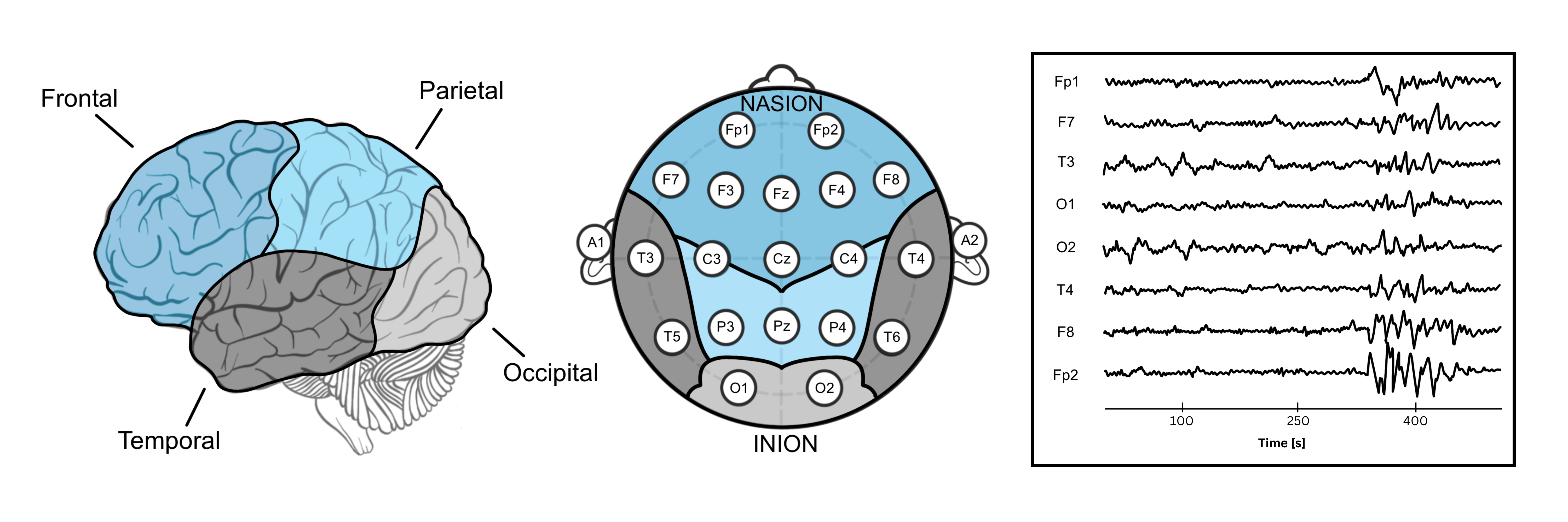
international 10–20 system for EEG (Klem et al., 1999). The labeling letters indicate the brain region covered by the electrodes. From front to the posterior part: Fp (pre-frontal or frontal pole), F (frontal), C (central line of the brain), T (temporal), P (parietal), and O (occipital). Sites marked with a “z” (zero) refer to an electrode placed on the midline sagittal plane of the skull (Fz, Cz, Pz). Electrodes labeled with an A are the earlobes, typically serving as an offline reference for signal analysis. These electrodes sometimes are placed on the mastoids, the bone behind the ear. Odd numbers represent electrodes on the left hemisphere, and even numbers represent electrodes on the right hemisphere; these numbers increase, as the electrodes move further from the midline. In addition, Figure 1 shows some examples of EEG signals recorded using the 10–20 system.

2.2 Multivariate extreme value theory

Let $\bm{X}_{d}:=\left(X_{d}^{1},\ldots,X_{d}^{T}\right)^{\intercal}$, $d=1,\ldots,D$, be the absolute amplitudes from the $d$-th EEG channel. We assume that $\bm{X}_{d}$ is a univariate stationary time series. We further assume the existence of real sequences $a_{d}^{T}>0$ and $b_{d}^{T}\in\mathbb{R}$, for each $d$, such that

$$\Pr\left(\frac{\max{\bm{X}_{1}}-b_{1}^{T}}{a_{1}^{T}}\leq x_{1},\ldots,\frac{\max{\bm{X}_{D}}-b_{D}^{T}}{a_{D}^{T}}\leq x_{D}\right)\stackrel{{\scriptstyle T\to\infty}}{{\longrightarrow}}G(x_{1},\ldots,x_{D}),$$ (1)

where $\max{\bm{X}_{d}}=\max{(X_{d}^{1},\ldots,X_{d}^{T})}$ is the componentwise maximum and $G$ is, in each margin, a non-degenerate distribution function.

According to the multivariate version of the extremal types theorem (de Haan and Ferreira, 2006), $G$ is a multivariate extreme-value distribution with generalized extreme value (GEV) margins. Specifically, each marginal distribution of the absolute amplitude of the EEG signal at each channel $d$ is given by

$$G_{d}(x;\,\mu_{d},\sigma_{d},\xi_{d})=\exp\left[-\left(1+\xi_{d}\frac{x-\mu_{d}}{\sigma_{d}}\right)^{-1/\xi_{d}}\right],\,\text{for}\,\,1+\xi_{d}\frac{x-\mu_{d}}{\sigma_{d}}>0,$$

where $\mu_{d}\in\mathbb{R}$ is the location parameter, $\sigma_{d}>0$ is the scale parameter, and $\xi_{d}\in\mathbb{R}$ is the extreme value index, a parameter characterizing the extreme behavior of component $d$.

The distribution $G_{d}$ belongs to either the Gumbel ($\xi_{d}=0$), the Fréchet ($\xi_{d}>0$) or the (reversed) Weibull ($\xi_{d}<0$) family. For illustration purposes, Figure 2 presents the probability density function

Figure 2: Illustration of a GEV distribution for location $\mu_{d}=0$ and scale $\sigma_{d}=1$. The varying values of the extreme value index give the three types of extreme-valued distributions under the GEV: Fréchet for $\xi_{d}=1/2$, (reversed) Weibull for $\xi_{d}=-1/2$, and Gumbel for $\xi_{d}=0$.

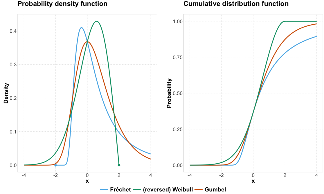
and cumulative distribution function for the three cases under $G_{d}(x;\,\mu_{d}=0,\sigma_{d}=1,\xi_{d}$), with $\xi_{d}=-1/2$ (Weibull), $0$ (Gumbel), $1/2$ (Fréchet). Note that we set the location ($\mu_{d}$) to zero, reason why we have negative values on the $x$-axis. The light-tailed Gumbel distribution is asymmetric and unbounded on both tails, i.e., its support is the whole real line. Extremes of exponential-type distributions, such as the Gaussian, lognormal, exponential, and gamma, converge to the Gumbel distribution. The heavy-tailed Fréchet distribution is also asymmetric but bounded to the left with support in $\left[\mu_{d}-\sigma_{d}/\xi_{d},\infty\right)$. Extremes from Pareto (power law) and Cauchy distributions converge to the Fréchet distribution. Finally, the short-tailed reversed Weibull distribution is bounded to the right with support in $\left(-\infty,\mu_{d}-\sigma_{d}/\xi_{d}\right]$. Extremes of the uniform converge to a reversed Weibull distribution.

Now, let $F_{d}(x)=\Pr(X^{t}_{d}<x)$ be the marginal distribution function of the stationary time series $\bm{X}_{d}$, $d=1,\ldots,D$. The convergence in Eq. (1) holds if, and only if, for any $t=1,\ldots,T$, the vector

$$\bm{Y}^{t}=\left(\left[1-F_{1}(X_{1}^{t})\right]^{-1},\ldots,\left[1-F_{D}(X_{D}^{t})\right]^{-1}\right)^{\intercal},$$ (2)

satisfies the regularly varying assumption

$$\dfrac{\bm{Y}^{t}}{\|\bm{Y}^{t}\|_{2}}\,\bigg{|}\,\|\bm{Y}^{t}\|_{2}>\tau\,\,\rightharpoonup\,\,S,\quad\tau\to\infty,$$ (3)

for a random vector $S$ with probability measure $\mathcal{S}$ on the (restricted) unit sphere $\mathbb{S}^{D-1}_{+}=\{\bm{s}\in\mathbb{R}^{D}_{+}:\|\bm{s}\|_{2}=1\}$, called the angular (or spectral) measure, where “$\|\cdot\|_{2}$” is the Euclidean norm and “$\rightharpoonup$” denotes weak convergence on $\mathbb{S}^{D-1}_{+}$. By definition, $\bm{Y}^{t}$ has unit Pareto margins; hence, if it satisfies Eq. (3), then it is in the maximum domain of attraction of a max-stable distribution with Fréchet margins and uniquely specified by the angular measure $\mathcal{S}$. Hence, the angular measure provides information on the dependence structure (or copula) of both maxima and exceedances of the multivariate standardized vector $\bm{Y}^{t}$, consequently also providing the same knowledge regarding $\bm{X}^{t}$ itself on the original scale.

2.3 Spherical $k$-means clustering algorithm

Our goal is to cluster EEG channels whose large (absolute) amplitudes in their signals are synchronized—either contemporaneous or with some time delay. To do so, we need to define the concept of asymptotic dependence (AD) and asymptotic independence (AI) between pairs of EEG signals. In the bivariate setting, the primary measure of asymptotic (in)dependence between two variables $Y_{d}$ and $Y_{d^{\prime}}$ defined through Eq. (2) is the tail correlation coefficient computed as

$$\chi_{dd^{\prime}}:=\lim\limits_{\tau\to\infty}\Pr\left(Y_{d^{\prime}}>\tau\mid Y_{d}>\tau\right)=\frac{1}{\mu}{\rm E}\left(S_{d}\wedge S_{d^{\prime}}\right)\in[0,1],\,d,d^{\prime}=1,\ldots,D,$$ (4)

where $\mu={\rm E}\left(S_{d}\right)$, $d=1,\ldots,D$. The case $\chi_{dd^{\prime}}=0$ corresponds to AI while $\chi_{dd^{\prime}}>0$ corresponds to AD. The link to the angular measure is that its distribution determines the occurrence of joint extremes. Suppose $\mathcal{S}$ has mass on a particular face of the sphere. In that case, this implies a positive probability that the corresponding variables experience extremes in synchrony (i.e., they are AD). In contrast, if $\mathcal{S}$ has no mass on a specific face, this implies AI for the corresponding variables. Our goal is to build a clustering algorithm such that channels are mutually AD within clusters (i.e., we are likely to observe high (absolute) amplitudes of all channels in synchrony) but AI across them.

To achieve our goal, we use a clustering procedure able to detect regions, in the faces of $\mathbb{S}_{+}^{D-1}$, where the mass of the angular measure is concentrated. That is, we need to group extreme observations with similar angles given by $\mathcal{S}$. There are two well-studied options in the literature: the spherical $k$–means (s–$k$–m) clustering algorithm by Janßen and Wan (2020) and the spherical $k$–principal–component (s–$k$–pc) clustering algorithm by Fomichov and Ivanovs (2022). In the former approach, similar observations are grouped into $k$ distinct clusters by minimizing a cosine dissimilarity, using an adaptation of the s–$k$–m algorithm by Dhillon and Modha (2001). Hence, the identified cluster centers can be thought of as angular prototypes for extremes, i.e., they reveal which directions of the extremes are the most likely. The latter is a two-step approach where a principal component analysis (PCA) suited for extremes (Drees and Sabourin, 2021) is combined with clustering. The first principal eigenvector is used to reduce the data dimensionality; then, a $k$-means algorithm with a quadratic dissimilarity measure is applied to identify the $k$ clusters.

Although, in practice, both approaches lead to similar results, the s–$k$–m method is computationally faster for complex high-dimensional data with a potentially larger number of clusters (Cheng, 2021). This is why, in this paper, we use the s–$k$–m algorithm. Nonetheless, in the Supplementary Material, we compare both methods in the context of our data analysis of Section 3.

In summary, we therefore aim to find $k$ centroids $\bm{a}_{c}\in\mathbb{R}_{+}^{D}$, $c\in\{1,\ldots,k\}$, such that the expected cosine dissimilarity of extreme observations to their closest cluster centroid is minimal. Hence, let $\{\bm{Y}^{t}\}_{t=1}^{T}$ be the multivariate time series of standardized (absolute) signals amplitudes given by Eq. (2). Assume we have $\mathcal{T}$ extreme observations above the threshold $\tau$ and let $\bm{\Theta}=\{\bm{\theta}^{1},\ldots,\bm{\theta}^{\mathcal{T}}\}$ be the pseudo-directions of such observations, with corresponding distribution $\mathcal{S}$ given by Eq. (3). Note that $\bm{\theta}^{t^{\prime}}\in\mathbb{R}_{+}^{D}$, $\forall t^{\prime}\in\{1,\ldots,\mathcal{T}\}$. Let $A=\{\bm{a}_{1},\ldots,\bm{a}_{k}\}\subset\mathbb{S}_{+}^{D-1}$ be the set of cluster centroids. Since the extreme (absolute) amplitudes are constrained to live on the unit sphere, the cosine dissimilarity can be used in its simplified version $\phi(\bm{\theta}^{t^{\prime}},\bm{a}_{c}):=1-\cos{({\bm{\theta}^{t^{\prime}}},\bm{a}_{c})}=1-{\bm{\theta}^{t^{\prime}}}^{\intercal}\bm{a}_{c}$, which is the spherical distance of the $t$-th extreme direction of $\bm{\Theta}$ to the centroid $\bm{a}_{c}\in A$. Hence, the minimized distance from arbitrary extreme observations, with directions $\bm{\theta}^{t^{\prime}}$, to their nearest cluster centroid on $A$ is $\varphi(\bm{\Theta},A):={\mathcal{T}}^{-1}{\sum\nolimits_{{t^{\prime}}=1}^{\mathcal{T}}{\min\nolimits_{\bm{a}_{c}\in A}\phi(\bm{\theta}^{t^{\prime}},\bm{a}_{c})}}$. Given $\bm{\Theta}$, we denote the optimal set minimizing $\varphi(\bm{\Theta},\cdot)$ as $A_{k}^{\mathcal{T}}$. The entire spherical clustering algorithm, embedded in the Club Exco method, is fully detailed in Section 2.5.

To illustrate how Club Exco works, Figure 3, panel A, shows three simulated EEG signals. Channels P4 and T6 are simulated under the moving average process of order 3 (MA(3)) $X^{t}=Z^{t}+0.5Z^{t-1}-0.6Z^{t-2}+1.5Z^{t-3}$, where $\{Z^{t}\}_{t=1}^{T}$ is an independent and identically distributed sequence of symmetric stable random variables with index $\alpha=1.75$ (Nolan, 2020). For illustration, set P4 and T6 as the time series given by $X^{t}$ and its lag-1 version, $X^{t-1}$, respectively. Hence, P4 and T6 are AD with $\chi\approx 0.28$, calculated empirically from Eq. (4) by taking the threshold $\tau$ as the empirical $0.998$–marginal quantile. Channel T3, on the other hand, is simulated, independently from P4 and T6, using the MA(4) process $X_{\star}^{t}=Z_{\star}^{t}+0.7Z_{\star}^{t-1}-0.2Z_{\star}^{t-2}+1.5Z_{\star}^{t-3}-0.5Z_{\star}^{t-4}$, where $Z_{\star}$ is obtained similarly as $Z$ with also $\alpha_{\star}=1.75$.

Figure 3: In panel A, simulated EEG signals from two AD channels (P4 and T6) and from one channel (T3) that is AI with the others. In panel B, extreme observations from the triplet (T3, P4, T6) are projected onto the unit positive octant suggesting AD between P4 and T6 but not with T3.

Therefore, T3 is AI with both P4 and T6. Figure 3, panel B, displays the 1% extreme (absolute) amplitudes of the triplet (T3, P4, T6) projected onto the unit positive octant. We apply the s–$k$–m algorithm with $k=2$ clusters to group these extreme observations. The two estimated clusters (gold and green points in panel B) suggest that channels P4 and T6 are indeed AD because the corresponding points (gold) on the sphere octant point toward joint extremes in both P4 and T6 but separately from T3. By contrast, channel T3 appears indeed to be AI with P4 and T6 because the correspondent points (green) point at extremes of T3 alone. Basically, the angles of the vectors pointing to the center of the gold and green points define the clusters’ centroids.

2.4 Frequency decomposition

In this section, we briefly discuss the frequency decomposition of brain signals. In neuroscience, it is common practice to decompose EEG signals into five canonical frequency bands, namely, delta (0–4 Hz), theta (4–8 Hz), alpha (8–12 Hz), beta (12–30 Hz), and gamma (30–50 Hz) bands. Each of these frequencies plays a different role in brain connectivity. For example, the gamma band is related to activities requiring focus and concentration; the beta band is associated with external attention; the alpha band accounts for passive attention and rest states, etc. (Abhang et al., 2016). Ombao and Pinto (in press) provide a review on EEG analysis in the frequency domain.

In addition to identifying clusters of concomitant extremes from the original brain signal, frequency-band-specific clusters can also be identified. For each canonical frequency band (delta, theta, alpha, beta, gamma), the original EEG signal is bandpass-filtered; amplitudes of the different oscillations are computed, and finally, clusters are determined according to the (absolute) amplitudes of the oscillations at each frequency band. Given the neurological interpretation of these frequency bands, it is likely that the clusters formed based on the extreme behavior of, say, the alpha band will differ from the clusters based on another frequency band.

2.5 Club Exco procedure

The procedure for applying Club Exco follows two steps described in Algorithms 1 and 2. In addition, one may work on either the amplitudes of the original time series or the bandpass-filtered time series to study frequency-specific tail dependence behaviors between channels.

In the first step, we identify the possible pseudo-directions of extreme observations as in Algorithm 1.

Data: A $T$-by-$D$ matrix $\bm{X}=[\bm{X}_{1},\ldots,\bm{X}_{D}]$ where columns contain the absolute signal amplitudes from the EEG channels or bandpass-filtered time series.

Result: Extreme directions $\bm{\Theta}=\{\bm{\theta}^{1},\ldots,\bm{\theta}^{\mathcal{T}}\}$.

begin

      

      1. Transform data on the original scale $\bm{X}$ to the unit Pareto scale $\bm{Y}$:

$$\bm{Y}^{t}\leftarrow\left(\left[1-F_{1}(X_{1}^{t})\right]^{-1},\ldots,\left[1-F_{D}(X_{D}^{t})\right]^{-1}\right),\;t=1,\ldots,T.$$

      2. For all $t\in\{1,\ldots,T\}$, keep the transformed observations with largest Euclidean norm:

$$\left\{{\bm{Y}^{*}}^{t^{\prime}}\right\}_{t^{\prime}=1}^{\mathcal{T}}\leftarrow\left\{\bm{Y}^{t}\,\big{|}\,\|\bm{Y}^{t}\|_{2}>\tau\right\}_{t=1}^{T}.$$

      3. Project the transformed observations onto the unit sphere:

$$\bm{\theta}^{t^{\prime}}\leftarrow\frac{{\bm{Y}^{*}}^{t^{\prime}}}{\|{\bm{Y}^{*}}^{t^{\prime}}\|_{2}},\;t^{\prime}=1,\ldots,\mathcal{T}.$$

end

Algorithm 1 Club Exco Algorithm 1: obtaining extreme directions.

In the second step, the s–$k$–m algorithm is applied to obtain the cluster centroids as in Algorithm 2.

Data: Extreme directions $\bm{\Theta}=\{\bm{\theta}^{1},\ldots,\bm{\theta}^{\mathcal{T}}\}$ and initial cluster centroids $A=\{\bm{a}_{1},\ldots,\bm{a}_{k}$}.

Result: Updated cluster centroids $A^{*}=\{\bm{a}^{*}_{1},\ldots,\bm{a}^{*}_{k}$} and minimized distance $\varphi(\bm{\Theta},A^{*})$.

repeat

       1. Assign $\bm{\theta}^{t^{\prime}}$ to the cluster with closest centroid $\bm{a}_{c}$, $c=1,\ldots,k$, by computing

$$\arg\min\nolimits_{\bm{a}_{c}\in A}\phi(\bm{\theta}^{t^{\prime}},\bm{a}_{c}),\,{t^{\prime}}=1,\ldots,\mathcal{T}.$$

      3. Update cluster centroids, $A$.

      

      2. Update the overall distance measure:

$$\varphi(\bm{\Theta},A)\leftarrow{\mathcal{T}}^{-1}{\sum\nolimits_{{t^{\prime}}=1}^{\mathcal{T}}{\min\nolimits_{\bm{a}_{c}\in A}\phi(\bm{\theta}^{t^{\prime}},\bm{a}_{c})}}.$$

until convergence;

Algorithm 2 Club Exco Algorithm 2: applying spherical $\bm{k}$–means.

3 Clustering multi-channel EEG seizure data

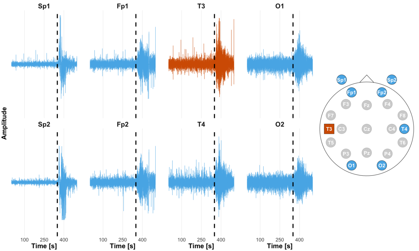
In this section, we analyze an EEG recording, from a female patient diagnosed with left temporal lobe epilepsy, which was first analyzed in Ombao et al. (2001). This recording captured the interictal (the period between seizures), pre-ictal (the period immediately before the seizure onset), and ictal phases (the period during the seizure episode). The recording is $T=500$ seconds and collected using 19 scalp electrodes placed following a $10$–$20$ system plus 2 sphenoidal intracranially electrodes at the base of the temporal lobe, resulting in $D=21$ EEG channels with a sampling rate of $100$ Hz. The electrodes follow a bipolar montage with a common reference between Cz and Pz. Figure 4 presents eight EEG channels and an illustration of the locations of the electrodes. The attending neurologist confirmed that the T3 channel (square) is the seizure onset zone (SOZ); the ictal onset was at $t=350$ second (vertical dashed line). This fact is corroborated by change point detection studies by Ombao et al. (2005), Schröder and Ombao (2019) and Jiao et al. (2021).

Figure 4: Selected EEG signals during an epileptic seizure (on a $10$–$20$ electrode system plus two sphenoidal electrodes placed intracranially at the base of the temporal lobe, namely, Sp1 and Sp2) from a female patient diagnosed with left temporal lobe epilepsy. The seizure onset (dashed vertical line) is roughly at $t=350$ seconds on the reference channel T3 (square). The EEG recording consists of $50,000$ time points at a sampling rate of $100$ Hz, i.e., $T=500$ seconds.

The main interest in this study is to identify groups of EEG channels for which high amplitudes in the signals are much more likely to occur together (with potential lead-lag between channels), i.e., we want to estimate clusters of asymptotically dependent channels. We refer to these clusters as brain extreme communities. In this analysis, the main goals of the neuroscientists are: (1.) to identify channels sharing the same extreme community as T3, the SOZ; (2.) to study how community memberships evolve through the seizure process; and (3.) to catalog differences in the extreme communities of varying frequency bands. In addition, we are interested in verifying whether extreme communities (based on the tails of the probability distribution) differ from clustering procedures based on the entire probability distribution, such as the HCC by Euán et al. (2019).

In a first analysis, the data are split into two distinct phases: pre-ictal (0–350 seconds) and ictal (350.01–500 seconds). We apply the Club Exco method separately for each phase to determine how seizure can alter brain extreme communities membership.

Figure 5: Estimated brain extreme communities considering $k=5$ clusters using the Club Exco approach for analyzing the EEG recording of a patient with left temporal lobe epilepsy during a seizure event. The seizure onset occurs at around second $t=350$ in a $T=500$ seconds recording. The threshold $\tau$ is set to the $0.90$ quantile.

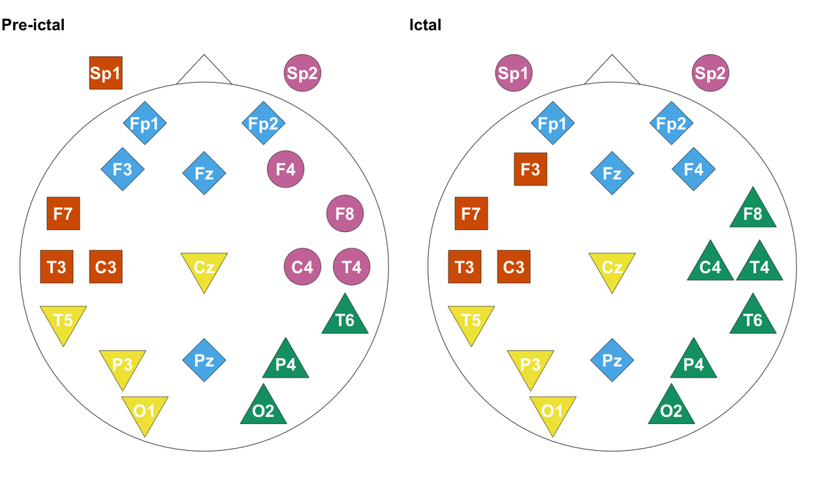
Figure 5 displays the estimated brain extreme communities considering $k=5$ clusters and the threshold $\tau$ as the $0.9$ quantile. In the Supplementary Material, we present a sensitivity analysis concerning the choice of both the number of clusters and threshold, and find that the results are fairly robust to this choice. From Figure 5, we conclude that after the seizure onset, the main change in brain extreme communities happens in the right hemisphere. The community previously formed by Sp2, F4, F8, C4, and T4 disappears. Channels F8, C4, and T4 are then connected to T6, P4, and O2. At the same time, channel F4 connects to the frontal channels (Fp1, Fp2, Fz) and Pz. The remaining channel, Sp2, is now connected to Sp1. Regarding T3, the SOZ, we have a minor difference between pre-ictal and ictal phases; its community loses connection to Sp1 but gains F3. Finally, the community formed by T5, P3, O1, and Cz stays the same after the seizure onset.

In a second analysis, we study the evolution of brain extreme communities over time by using sliding windows. All EEG signals are split into $W=50$ disjoint sliding windows of $10$ seconds in length. This is the strategy used by Euán et al. (2019) while clustering channels based on the same dataset. We followed their procedure in order to contrast their results with Club Exco results (see the discussion regarding Figures 7 and 8 at the end of this section). Before comparing both methods, we focus on the time evolution of Club Exco only. For each sliding window, we apply the Club Exco procedure, and then, taking all windows before the seizure onset, we counted the number of times each pair of channels belong to the same brain extreme community. The same is done for all windows after the seizure onset. Figure 6 displays the extreme connectivity persistence over time, i.e., it represents the percentage of time two given channels belong to the same brain extreme community.

Figure 6: Percentage of time two given channels belong to the same brain extreme community (i.e., extreme connectivity persistence) using the Club Exco approach for $k=5$ clusters. Results are based on $W=50$ disjoint sliding windows (of 10-seconds duration) over the entire EEG recording from a patient during a seizure event. The seizure onset is placed at second $t=350$. For all sliding windows, the threshold $\tau$ is set to the $0.90$ quantile.

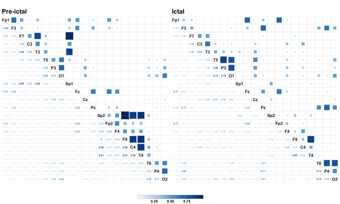
Prior to the ictal phase, there were more pairs of channels with high persistence. The right hemisphere has more persistence than the left hemisphere, with channels F8 and Sp2 connected all the time. In addition, the community formed by channels Sp2, F8, C4, and T4 is highly persistent. Similarly, in the left hemisphere, the channels on the same topographical level, i.e., Sp1, F7, C3, and T3, are also highly persistent. An interesting observation is that before the seizure onset, the right and left hemispheres have “mild local-mirrored communication”, i.e., left and right channels opposed to midline are the only channels sharing a brain extreme community. Note the community formed by T5, P3, and O1 on the left side together with T6, P4, and O2 on the right side. Another of these communities is formed by Fp1 and F3 (on the left) plus Fp2 and F4 (on the right). On the other hand, these local communities grouping the right and left hemispheres are disrupted during the ictal phase; postseizure onset, we have “mild global communication” between the two hemispheres, i.e., channels from all regions in the left and right hemispheres communicate. Some examples: (a.) Fp1 with Fp2; (b.) F3 with T6, P4, and O2; (c.) C3 with F4 and C4; and (d.) O1 with F4, C4, T6, and O2. Now, focusing on T3, before the seizure onset, there is strong connectivity persistence with channels Sp1 (0.85), F7 (0.82), and C3 (0.56). After the seizure onset, only channel C3 has strong connectivity persistence with T3 (0.64).

In a final analysis, we decompose the channels into canonical frequency bands, analyzing them separately. Considering the alpha and beta bands, we compare Club Exco results to the HCC results of Euán et al. (2019). We select three specific sliding windows to contrast the results. The first window is an interictal phase, going from 40 to 50 seconds (sliding window 5); the second window represents a pre-ictal phase, from 340 to 350 seconds (sliding window 35); while the third window lies in the ictal phase, from 370 to 380 seconds (sliding window 38). As Euán et al. (2019) explain, there is no clear way of labeling the changing clusters since two clusters from different time segments do not necessarily contain identical members even if $k$ remains the same. Hence, since T3 (square) is of particular interest being the SOZ, we single out its extreme community by coloring it in orange (diamonds) in Figures 7 and 8; then, we group all other communities not having T3 as a single community, coloring it in cyan (circles). Before proceeding with the analysis, it is essential to mention that, given the HCC method’s hierarchical structure, Euán et al. (2019) use a different number of clusters for each seizure phase and frequency band, as seen in Table 1. To make a fair comparison, we adopt the same approach for Club Exco in this final analysis.

Table 1: Number of clusters for each seizure phase for alpha and beta bands.

	interictal	pre-ictal	ictal
alpha band	6	7	5
beta band	6	8	6

Figure 7 contrasts results between Club Exco and HCC for the alpha band. There is a distinct behavior between the two clustering methods. The extreme communities containing T3,

Figure 7: Clustering results for alpha band (8–12 Hz). Connectivity with T3 based on: (a.) the tails of the probability distribution (Club Exco; top-panel line); and (b.) the entire probability distribution (HCC; bottom-panel line). The time window for each moment are 40 to 50 sec (interictal; $k=6$), 340 to 350 sec (pre-ictal; $k=7$), and 370 to 380 sec (ictal; $k=5$).

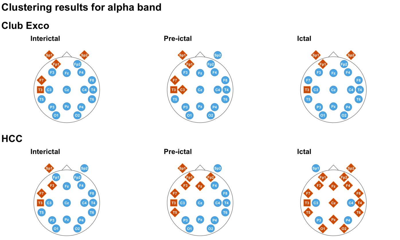
estimated by Club Exco, remain relatively stable regarding the number of its elements (interictal: 5, pre-ictal: 5, and ictal: 4), while HCC clusters grow in the power of 2 (interictal: 4, pre-ictal: 8, and ictal: 16). In general, when studying a seizure episode considering the entire probability distribution, the seizure spreads and generalizes as it progresses. However, the seizure does not generalize to the whole brain when focusing only on the distribution’s tails. To clarify this point, in the Supplementary Material, we include a video with the time-lapse of all 50 sliding windows considering the original signal and both the alpha and beta bands. With Club Exco, channels Fp1 and Sp1 are always in the extreme community of T3. As to HCC, it is F7 and F3 that are always in the same cluster as T3. In the alpha band, as the seizure process advances, most channels become increasingly coherent with T3 when data from the entire probability distribution is analyzed. However, when only data from the tails are studied, we do not observe such a strong agreement; only a few channels are asymptotically dependent with T3.

Figure 8 shows the same results but for the beta band, which has a higher frequency than the alpha band. Here, we can see a much more similar behavior between the two methods.

Figure 8: Clustering results for beta band (12–30 Hz). Connectivity with T3 based on: (a.) the tails of the probability distribution (Club Exco; top-panel line); and (b.) the entire probability distribution (HCC; bottom-panel line). The time window for each moment are 40 to 50 sec (interictal; $k=6$), 340 to 350 sec (pre-ictal; $k=8$), and 370 to 380 sec (ictal; $k=6$).

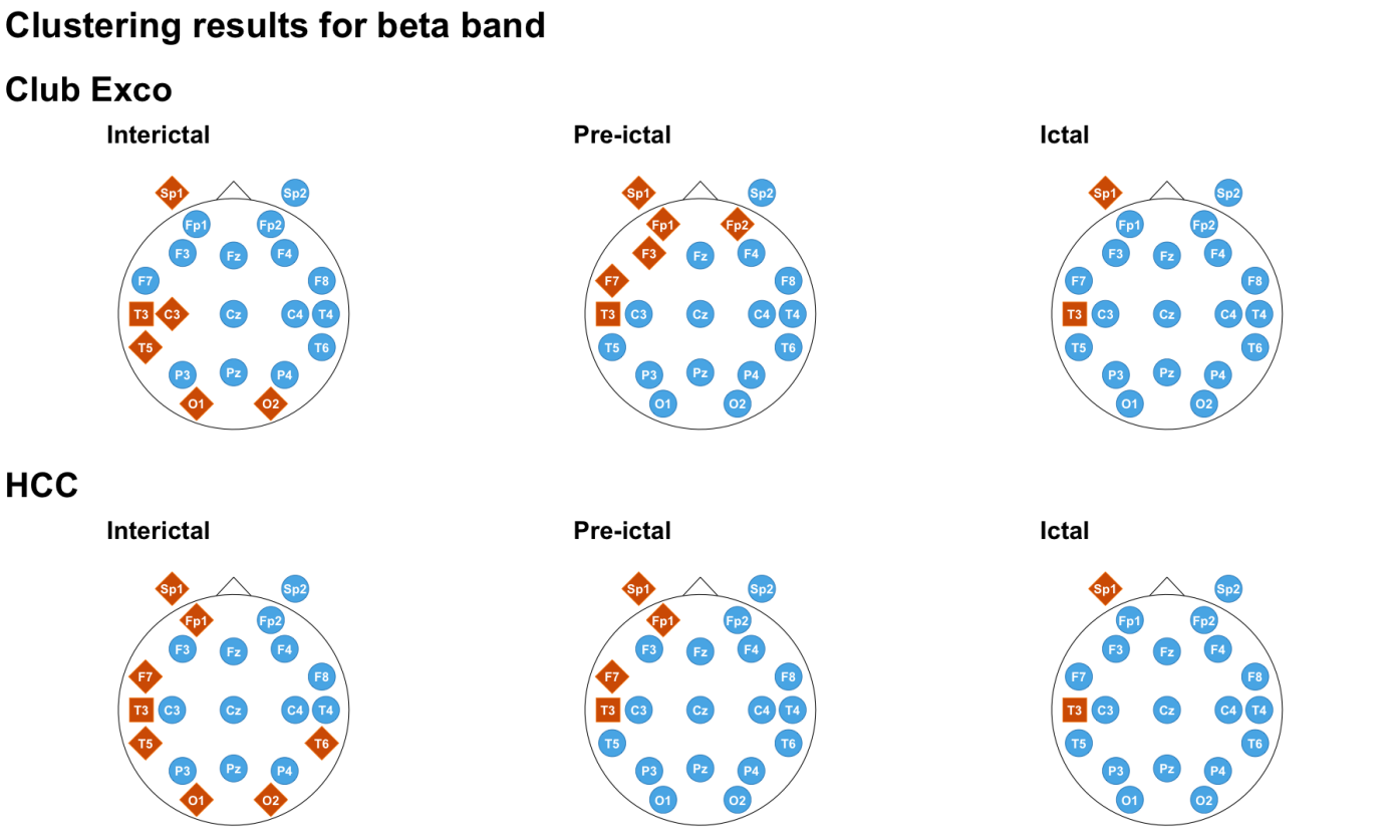
In addition, unlike in the alpha-band case, fewer channels are connected with T3 as the seizure process advances for both Club Exco (interictal: 6, pre-ictal: 6, and ictal: 2) and HCC (interictal: 8, pre-ictal: 4, and ictal: 2). Note that Sp1 is always connected with T3 for both methods, meaning this channel follows T3 in the bulk and tails of the probability distribution.

In the Supplement Material, we present similar plots (in a time-lapse video) considering the brain extreme communities having T4, Sp1, Sp2, O1, and O2 as members. Hence we can compare results with T3. We notice that T3, despite being the seizure focus, does not play a unique role in the extreme behavior of the brain during the seizure episode. Brain extreme communities seem localized, respecting the left-right and frontal-occipital regions.

4 Conclusions and future work

This paper highlights the importance of studying brain connectivity from different perspectives. Here, we offer a new perspective that is grounded by extreme value theory to characterize brain connectivity. Our method, Club Exco, has the unique ability to identify brain extreme communities, i.e., clusters of EEG channels sharing the same extremal behavior. The novel elements of the Club Exco method are that clusters reflect channels that are mutually asymptotically dependent (AD), meaning they all are likely to experience extreme (absolute) amplitudes synchronously or at some short time lag. This feature is the main advantage of Club Exco. We contrast our methodology with the non-EVT-based method HCC, which clusters channels based on the notion of coherence. In this approach, two EEG channels belong to the same cluster if their entire probability distributions similarly reflect the same neurological phenomenon.

The Club Exco method produced novel appealing results. Our analysis identified different patterns in the alpha band (8–12 Hz), especially during the ictal phase (a few seconds postseizure onset). The competitor method, HCC, suggests that almost all EEG channels (15 out of 20) are coherent with T3, the left temporal channel, which is the seizure onset zone. Club Exco captures a very distinctive portrait of connectivity during the ictal phase. At the tails of the (absolute) amplitudes, only three channels are synchronized with T3. In contrast, in the beta band (12–30 Hz) case, both methods produce clusters much more alike regarding all three seizure phases. These discrepancies emphasize that different methods capture distinct facets of brain connectivity. All these facets are essential to understanding the seizure process as a whole. In this context, we conjecture that Club Exco is showing which regions (or which portion of the network) is actually generating the seizure activity, as opposed to the regions that are later recruited into the seizure (but are not generating or driving the activity). We hope to investigate it in more detail in future work, with the analysis of multi-subject datasets.

Furthermore, different neurological questions may demand distinct statistical methods for more precise answers. As statisticians and data scientists, our role is to uncover as many features as possible from the data to assist neuroscientists and neurologists better. Here, we are pleased to include a hitherto missing piece in this statistical Swiss Army knife for brain connectivity studies: Club Exco, a tool capturing the facet of extremal connectivity during an epileptic episode.

This work will be extended to modeling multi-subject seizure data, comparing the differences in brain extreme communities between epileptic patients and healthy controls. We also aim to develop a data-driven automatic method for selecting the optimal number of clusters that takes into consideration non-stationarity in the signals (and hence the number may potentially vary across time) and the clustering across different dimensions (clustering of channels; clustering of subjects).

For reproducibility purposes and to make our methodology more accessible to the whole community, the data can be obtained upon reasonable request from the authors, and we will make our R code available for download from the following first author’s GitHub repository: https://github.com/matheusguerrero/club-exco (see also the Supplementary Material for a smaller toy example).

References

- Abhang et al. (2016) P. A. Abhang, B. W. Gawali, and S. C. Mehrotra. Chapter 2 - Technological basics of EEG recording and operation of apparatus. In P. A. Abhang, B. W. Gawali, and S. C. Mehrotra, editors, Introduction to EEG and Speech-based Emotion Recognition, pages 19–50. Academic Press, 2016.
- Barnett et al. (2018) L. Barnett, A. B. Barrett, and A. K. Seth. Solved problems for Granger causality in neuroscience: A response to Stokes and Purdon. NeuroImage, 178:744–748, 2018.
- Biswas and Ombao (2022) A. Biswas and H. Ombao. Frequency–specific non–linear Granger causality in a network of brain signals. In ICASSP 2022–2022 IEEE International Conference on Acoustics, Speech and Signal Processing (ICASSP), pages 1401–1405, 2022.
- Cascino et al. (2021) G. D. Cascino, J. I. Sirven, and W. O. Tatum. Epilepsy. Wiley-Blackwell, UK, 2 edition, 2021.
- Cheng (2021) J. Cheng. Clustering methods of multivariate extremes: a model comparison analysis with empirical case studies. Bachelor’s thesis, Erasmus University Rotterdam, School of Economics, Netherlands, 2021.
- Daouia et al. (2019) A. Daouia, I. Gijbels, and G. Stupfler. Extremiles: a new perspective on asymmetric least squares. Journal of the American Statistical Association, 114:1366–1381, 2019.
- Davison and Huser (2015) A. C. Davison and R. Huser. Statistics of extremes. Annual Review of Statistics and Its Application, 2(1):203–235, 2015.
- Davison et al. (2019) A. C. Davison, R. Huser, and E. Thibaud. Spatial extremes. In A. E. Gelfand, M. Fuentes, J. A. Hoeting, and R. L. Smith, editors, Handbook of Environmental and Ecological Statistics, chapter 31, pages 711–744. CRC Press, Boca Raton, FL, 2019.
- de Haan and Ferreira (2006) L. de Haan and A. Ferreira. Extreme Value Theory: An Introduction. Springer Series in Operations Research and Financial Engineering. Springer, New York, 2006.
- Dhillon and Modha (2001) I. S. Dhillon and D. S. Modha. Concept decompositions for large sparse text data using clustering. Machine Learning, 42:143–175, 2001.
- Drees and Sabourin (2021) H. Drees and A. Sabourin. Principal component analysis for multivariate extremes. Electronic Journal of Statistics, 15:908–943, 2021.
- Einmahl and Smeets (2011) J. H. J. Einmahl and S. G. W. R. Smeets. Ultimate 100-m world records through extreme-value theory. Statistica Neerlandica, 65:32–42, 2011.
- Embleton et al. (in press) J. Embleton, M. I. Knight, and H. Ombao. Multiscale modelling of replicated nonstationary time series. The Annals of Applied Statistics, in press.
- Engelke and Ivanovs (2021) S. Engelke and J. Ivanovs. Sparse structures for multivariate extremes. Annual Review of Statistics and its Application, 8(1):241–270, 2021.
- Euán et al. (2019) C. Euán, Y. Sun, and H. Ombao. Coherence-based time series clustering for statistical inference and visualization of brain connectivity. The Annals of Applied Statistics, 13(2):990–1015, 2019.
- Fomichov and Ivanovs (2022) V. Fomichov and J. Ivanovs. Spherical clustering in detection of groups of concomitant extremes. Biometrika, 00(0):1–19, 2022.
- Freyer et al. (2009) F. Freyer, K. Aquino, P. A. Robinson, P. Ritter, and B. Breakspear. Bistability and non-Gaussian fluctuations in spontaneous cortical activity. Journal of Neuroscience, 29:8512–8524, 2009.
- Fryzlewicz and Ombao (2009) P. Fryzlewicz and H. Ombao. Consistent classification of nonstationary time series using stochastic wavelet representations. Journal of the American Statistical Association, 104(485):299–312, 2009.
- Gong and Huser (2022) Y. Gong and R. Huser. Asymmetric tail dependence modeling, with application to cryptocurrency market data. The Annals of Applied Statistics, 16(3):1822–1847, 2022.
- Guerrero et al. (2022+) M. B. Guerrero, R. Huser, and H. Ombao. Conex-connect: Learning patterns in extremal brain connectivity from multi-channel EEG data. The Annals of Applied Statistics, 2022+. In press.
- Janßen and Wan (2020) A. Janßen and P. Wan. -means clustering of extremes. Electronic Journal of Statistics, 14(1):1211–1233, 2020.
- Jiao et al. (2021) S. Jiao, T. Shen, Z. Yu, and H. Ombao. Change-point detection using spectral PCA for multivariate time series. arXiv e-prints, art. arXiv:2101.04334, 2021.
- Kaya (2021) I. Kaya. A brief summary of EEG artifact handling. In Vahid Asadpour, editor, Brain-Computer Interface, chapter 2. IntechOpen, Rijeka, 2021.
- Klem et al. (1999) G. H. Klem, H. O. Lüders, H. H. Jasper, and C. Elger. The ten-twenty electrode system of the international federation. The international federation of clinical neurophysiology. Electroencephalography and Clinical Neurophysiology – Supplement, 52:3–6, 1999.
- Maulik et al. (2002) K. Maulik, S. Resnick, and H Rootzén. Asymptotic independence and a network traffic model. Journal of Applied Probability, 39:671–699, 2002.
- Murugappan (2010) M. Murugappan. Classification of human emotion from EEG using discrete wavelet transform. Journal of Biomedical Science and Engineering, 3:390–396, 2010.
- Nolan (2020) J.P. Nolan. Univariate Stable Distributions: Models for Heavy Tailed Data. Springer Series in Operations Research and Financial Engineering. Springer, New York, 2020.
- Ombao and Pinto (in press) H. Ombao and M. Pinto. Spectral dependence. Econometrics and Statistics, in press.
- Ombao et al. (2001) H. Ombao, J. A. Raz, R. von Sachs, and B. A. Malow. Automatic statistical analysis of bivariate nonstationary time series. In memory of Jonathan a. Raz. Journal of the American Statistical Association, 96(454):543–560, 2001.
- Ombao et al. (2005) H. Ombao, R. von Sachs, and W. Guo. SLEX analysis of multivariate nonstationary time series. Journal of the American Statistical Association, 100:519–531, 2005.
- Ombao et al. (2016) H. Ombao, M. Lindquist, Thompson W., and J. Aston. Handbook of Neuroimaging Data Analysis. Chapman and Hall/CRC, USA, 2016.
- Orsini et al. (2019) F. Orsini, G. Gecchele, M. Gastaldi, and R. Rossi. Collision prediction in roundabouts: a comparative study of extreme value theory approaches. Transportmetrica A: Transport Science, 15:556–572, 2019.
- Park et al. (2014) T. Park, I. Eckley, and H. Ombao. Estimating the time–evolving partial coherence between signals via multivariate locally stationary wavelet processes. IEEE Transactions on Signal Processing, 62:5240–5250, 2014.
- Richards and Huser (2022) J. Richards and R. Huser. A unifying partially-interpretable framework for neural network-based extreme quantile regression. arXiv e-prints, art. arXiv:2208.07581, 2022.
- Roberts et al. (2015) J. A. Roberts, T. W. Boonstra, and M. Breakspear. The heavy tail of the human brain. Current Opinion in Neurobiology, 31:164–172, 2015.
- Rudd et al. (2018) E. M. Rudd, L. P. Jain, W. J. Scheirer, and T. E. Boult. The extreme value machine. IEEE Transactions on Pattern Analysis and Machine Intelligence, 40(3):762–768, 2018.
- Sabourin (2021) A. Sabourin. Extreme Value Theory and Machine Learning. Accreditation to supervise research, Institut Polytechnique de Paris, France, 2021.
- Sazgar and Young (2019) M. Sazgar and M. G. Young. Absolute Epilepsy and EEG Rotation Review: Essentials for Trainees. Springer, USA, 2019.
- Schröder and Ombao (2019) A. L. Schröder and H. Ombao. FreSpeD: frequency-specific change-point detection in epileptic seizure multi-channel EEG data. Journal of the American Statistical Association, 114:115–128, 2019.
- Seth et al. (2015) A. K. Seth, A. B. Barrett, and L. Barnett. Granger causality analysis in neuroscience and neuroimaging. Journal of Neuroscience, 35(8):3293–3297, 2015.
- Spencer et al. (2018) E. Spencer, L.-E. Martinet, E.N. Eskandar, C.J. Chu, E.D. Kolaczyk, S.S. Cash, U.T. Eden, and M.A. Kramer. A procedure to increase the power of Granger-causal analysis through temporal smoothing. Journal of Neuroscience Methods, 308:48–61, 2018.
- Spencer et al. (2003) K. M. Spencer, P. G. Nestor, M. Niznikiewicz, D. F. Salisbury, M. E. Shenton, and R. W. McCarley. Abnormal neural synchrony in schizophrenia. Journal of Neuroscience, 23:7407–7411, 2003.
- Tsai et al. (2010) Y. T. Tsai, H. L. Chan, S. T. Lee, P. H. Tu, B. L. Chang, and T. Wu. Significant thalamocortical coherence of sleep spindle, theta, delta, and slow oscillations in NREM sleep: recordings from the human thalamus. Neuroscience Letters, 485:173–177, 2010.
- Tsinos et al. (2018) C. G. Tsinos, F. Foukalas, T. Khattab, and L. Lai. On channel selection for carrier aggregation systems. IEEE Transactions on Communications, 66:808–818, 2018.
- Übeyli (2008) E. D. Übeyli. Wavelet/mixture of experts network structure for EEG signals classification. Expert Systems with Applications, 34:1954–1962, 2008.
- van Luijtelaar et al. (2011) G. van Luijtelaar, A. Hramov, E. Sitnikova, and A. Koronovskii. Spike-wave discharges in wag/rij rats are preceded by delta and theta precursor activity in cortex and thalamus. Clinical Neurophysiology, 122:687–695, 2011.
- WHO (2019) WHO. Epilepsy: a public health imperative - summary. https://www.who.int/mental_health/neurology/epilepsy/report_2019/en/, 2019. Accessed on 15/09/2022.
- Wong and Collins (2020) F. Wong and J. J. Collins. Evidence that coronavirus superspreading is fat-tailed. Proceedings of the National Academy of Sciences of the United States of America, 117:29416–29418, 2020.