Unpredictability in seasonal infectious diseases spread

Abstract

In this work, we study the unpredictability of seasonal infectious diseases considering a SEIRS model with seasonal forcing. To investigate the dynamical behaviour, we compute bifurcation diagrams type hysteresis and their respective Lyapunov exponents. Our results from bifurcations and the largest Lyapunov exponent show bistable dynamics for all the parameters of the model. Choosing the inverse of latent period as control parameter, over 70% of the interval comprises the coexistence of periodic and chaotic attractors, bistable dynamics. Despite the competition between these attractors, the chaotic ones are preferred. The bistability occurs in two wide regions. One of these regions is limited by periodic attractors, while periodic and chaotic attractors bound the other. As the boundary of the second bistable region is composed of periodic and chaotic attractors, it is possible to interpret these critical points as tipping points. In other words, depending on the latent period, a periodic attractor (predictability) can evolve to a chaotic attractor (unpredictability). Therefore, we show that unpredictability is associated with bistable dynamics preferably chaotic, and, furthermore, there is a tipping point associated with unpredictable dynamics.

1 Introduction

The study of the spread of diseases is an important interdisciplinary research topic [1]. Mathematical models are essential to understanding, forecasting, and studying control measures for infectious diseases spread [2]. In general, the epidemic models are compartmental, i.e., they divide the host population ($N$) into compartments, for instance susceptible ($S$), exposed ($E$), infected ($I$), and recovered ($R$) [3]. $S$ is related to healthy individuals who can contract the disease. $E$ corresponds to the individuals in latent [4] and/or incubation period [5]. In the latent period, the individuals can not transmit the disease [2]. In the incubation period, the exposed can transmit the disease with a lower incidence than the infected individuals [6, 7]. $I$ is associated with individuals who transmit the disease. $R$ is related to the individuals who were infected and got immunity, permanent [2] or temporary [8]. The composition of these compartments forms the classical epidemics models: Susceptible-Infected (SI) [9], Susceptible-Infected-Susceptible (SIS) [10], Susceptible-Infected-Recovered (SIR) [11], Susceptible-Infected-Recovered-Susceptible (SIRS) [12], Susceptible-Exposed-Infected-Recovered (SEIR) [13, 2], and Susceptible-Exposed-Infected-Recovered-Susceptible (SEIRS) [8]. An introduction to these models can be found in Ref. [3]. These models have been used to study the dynamic of many diseases, for example, COVID-19 [14], dengue fever [15], and childhood epidemics (e.g., measles, diphtheria, and chickenpox) [16].

Some of these diseases have seasonal behaviour, like measles, chickenpox, pertussis, and others [17, 18]. The common characteristic of seasonal diseases is the recurrence of new outbreaks after a period of time. The motivation to work with seasonal models is to predict future outbreaks and propose control measures [19].

Seasonal models have been introduced since 1928 [20]. They present a rich variety of oscillatory phenomena [21]. London and Yorke [22] considered an epidemic model with seasonally varying contact rates forcing, studied the recurrent outbreaks of measles, chickenpox, and mumps in New York City. Their simulations reproduced the observed pattern in annual outbreaks of chickenpox, mumps and biennial outbreaks of measles and also verified that the mean contact rate is higher in winter than in summer. Considering a SEIR model with seasonal components, Olsen and Schaffer [16] showed, from real data, that measles epidemics are inherently chaotic. Aguiar et al. [23] analysed a seasonally forced SIR epidemic model for dengue fever with temporary cross-immunity and the possibility of secondary infection. Their results showed that the addition of seasonal forcing induces chaotic dynamics, which is related to the decrease in predictability. Similar results in a SIR model were reported by Stollenwerk et al. [24]. He et al. [25] explored a SEIR epidemic model based on the COVID-19 data from Hubei province. With the introduction of seasonality and stochastic infection, the model becomes nonlinear with chaos. In addition to this work, from the analysis of epidemiological data from 14 countries, the work of Jones and Strigul [26] suggested that the COVID-19 spread is chaotic. Bilal et al. [27] studied changes in the bifurcations of the seasonally forced SIR model considering a transmission rate modulated temporally. By analysing the bifurcation diagrams and respective Lyapunov exponents, in the forward and backward directions of the strength of seasonality, their results showed the coexistence between periodic and chaotic attractors, known as bistability dynamics. Bistability in an epidemic model also was reported by Ventura et al. [28]. They considered a model with mobility where the spreading of disease occurs in temporal networks of mobile agents. In their model, they considered the movement of susceptible in the oppositive direction of infected agents. By developing a semi-analytic approach, they showed that the bistability is caused by the spatial emergence of susceptible clustering.

Many natural processes exhibit multistability, i.e., the asymptotic state evolves to a large number of coexistence attractors for a fixed parameter set [29]. In these systems, the transient for the final attractor depends strongly on the initial condition [30, 31]. The existence of two alternative states is very important to climate science [32], ecology [33], and epidemiology [11, 27, 28]. When the multistability region is bounded by contrasting attractors and an abrupt shift between these attractors occurs, the threshold points in which this transition occurs are called tipping points [34].

Tipping points are found in the process of desertification [34], cancer epidemiology [35], Duffing oscillator [36], epidemic models [37, 38, 39], ecological models [40], and others [41]. Mathematically, the tipping points correspond to bifurcations [34], that, in general, have long transient lifetimes [42]. In the ecological sense, long transients were studied by Hastings et al. [43].

In seasonal disease spread, an unclear problem is the limit to forecast precision for the outbreak, as observed by Scarpino and Petri [44]. They studied the time series from ten different diseases (for example, dengue, influenza, measles, and mumps) and demonstrated that the predictability decreases when the time series length is increased. Furthermore, their results showed that the forecast horizon varies by different illnesses. From the other works, it is known that unpredictability is associated with the chaotic dynamics [45]. However, only chaotic dynamics do not provide a satisfactory answer to understanding the mechanism behind unpredictability, since the chaotic attractors are predictable until a Lyapunov time in the order to the inverse of the largest Lyapunov exponent.

Our main goal in this research is to study the mechanism behind the unpredictability in seasonal infectious diseases. In order to that, we consider a SEIR model with temporary immunity and seasonal forcing [46, 47]. Firstly, we show that the basic reproductive rate $R_{0}$ depends on the seasonality parameters, such as seasonality degree and frequency. In sequence, we consider numerical simulations which exhibit the existence of bistability for all parameters in the model, which is characterised by the coexistence of periodic and chaotic attractors. We verify this dynamical behaviour by bifurcations diagram type hysteresis and the largest Lyapunov exponent. Despite the rich dynamics in all the parameters, we select the inverse of the latent period to study the unpredictability phenomenon. A wide range of this parameter comprises diseases with short (hours) and large (days) latent period. Our results show that the dynamics are sustained over 70% by bistability between chaotic and periodic attractors. This bistability appears in two large ranges. In the first one, the probability of one initial condition evolving to the chaotic attractor is 51%, while in the second range is 63%. Furthermore, these two ranges are delimited, in their crisis points, by periodic and chaotic attractors (without bistability). In this sense, it is possible to interpret these bifurcations as tipping points. In this way, as novelty, we exhibit that the unpredictability in infectious disease spread is associated with bistable dynamics and exists one tipping point associated with it.

Our work is organised as follows: In section 2, we present the model. Section 3 is dedicated for the study of bifurcations and crisis points. In Section 4, we interpret the crisis points as tipping points. Finally, in Section 5, we draw our conclusions.

2 Model

The SEIRS model divides the host population ($N$) into four compartments [2, 3, 8]: $S$, $E$, $I$, and $R$. A schematic representation of the SEIRS model is shown in Fig. 1. The $R$ individuals lose immunity after a period time given by $1/\delta$ and return to $S$ compartmental. The model is given by

$$\begin{split}\frac{dS}{dt}&=bN(t)-\mu S(t)-\beta\frac{S(t)I(t)}{N(t)}+\delta R(t),\\ \frac{dE}{dt}&=\beta\frac{S(t)I(t)}{N(t)}-(\alpha+\mu)E(t),\\ \frac{dI}{dt}&=\alpha E(t)-(\gamma+\mu)I(t),\\ \frac{dR}{dt}&=\gamma I(t)-\mu R(t)-\delta R(t),\\ \end{split}$$ (1)

where $b$ is the natural birth rate, $\mu$ is the natural death rate, $\alpha$ is the rate at which exposed individuals evolve to be infected, $\gamma$ is the recovered rate, $\delta$ is the rate at which the recovered individuals return to the susceptible class after losing immunity. The mean latent period is given by $1/\alpha$, the mean infectious period by $1/\gamma$, and the mean time immunity by $1/\delta$. The force of infection is $\frac{\beta I}{N}$, where $\beta$ is the effective per capita contact rate of infective individuals and the incidence rate is $\frac{\beta SI}{N}$.

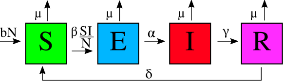
Figure 1: Schematic representation of SEIRS model, where $N$ is the host population, $b$ is the natural birth rate, $\mu$ is the natural death rate, $\beta$ is the effective per capita contact rate, $\alpha$ is the rate at which $E$ evolves to $I$, $\gamma$ is the recovered rate, $\delta$ is the rate in which $R$ return to $S$ compartmental.

We consider the transmission rate with a seasonal forcing given by

$$\beta(t)=\beta_{0}(1+\beta_{1}{\rm cos}\omega t),$$ (2)

where $\beta_{0}$ is the average contact rate, $\beta_{1}$ ($0\leq\beta_{1}\leq 1$) measures the seasonality degree, and $\omega$ is the frequency [16, 46, 47]. Considering $\mu=b$, we obtain, from Eq. LABEL:eq1, $S+E+I+R=N$. Therefore, it is possible, without loss of generality, to rewrite Eq. LABEL:eq1 using the following transformations: $s=S/N$, $e=E/N$, $i=I/N$, $r=R/N$.

The equilibrium solutions of SEIRS model are found by solving the following equations

$$\begin{split}0&\equiv b-\mu s-\beta si+\delta r,\\ 0&\equiv\beta si-(\alpha+\mu)e,\\ 0&\equiv\alpha e-(\gamma+\mu)i,\\ 0&\equiv\gamma i-\mu r-\delta r,\end{split}$$ (3)

where the disease-free equilibrium is $(s^{*},e^{*},i^{*},r^{*})=(1,0,0,0)$, since $b=\mu$. However, a very important equilibrium solution is the endemic solution, which is given by

$$\begin{split}s^{*}&=\frac{(\alpha+\mu)(\gamma+\mu)}{\beta(t)\alpha}\equiv\frac{1}{R_{0}},\\ e^{*}&=\frac{\gamma+\mu}{\alpha}\frac{\mu+\delta}{\beta(t)(\mu+\delta)-R_{0}\delta\gamma}(bR_{0}-\mu),\\ i^{*}&=\frac{\mu+\delta}{\beta(t)(\mu+\delta)-R_{0}\delta\gamma}(bR_{0}-\mu),\\ r^{*}&=1-s^{*}-e^{*}-i^{*},\end{split}$$ (4)

where $R_{0}$ is the basic reproductive ratio [48]. We consider $\mu=b$ to obtain a fixed population size. If $\delta=0$ and $\mu=b$, we recover the expression $i^{*}=\frac{\mu}{\beta}(R_{0}-1)$ that is the endemic fixed point for the SEIR model, as shown in Ref. [48] without seasonal forcing. In this way, the terms $\delta$, $b$, $\gamma$, $\beta_{0}$, and $\beta_{1}$ appear as correction terms in the infected individuals. $R_{0}=R_{0}(t)\propto\beta_{0}(1+\beta_{1}{\rm cos}\omega t)$ is proportional to the seasonal parameters.

However, Eq. 2 makes the system become nonautonomous. To build an autonomous system, we introduce a new variable $T=\omega t$ and a new differential equation, that is given by $\frac{dT}{dt}=\omega$. With these considerations, the equations become

$$\begin{split}\frac{ds}{dt}&=\mu-\mu s-\beta(T)si+\delta r,\\ \frac{de}{dt}&=\beta(T)si-(\alpha+\mu)e,\\ \frac{di}{dt}&=\alpha e-(\gamma+\mu)i,\\ \frac{dT}{dt}&=\omega,\\ r&=1-s-e-i,\end{split}$$ (5)

where the differential equation for $r$ is replaced by the constraints. As an example, a solution of Eq. 5 is shown in Fig. 2(a) for all variables. Differently from the standard SEIRS, the seasonal forcing produces oscillations in the epidemic curves in accordance with $\omega$. The exposed and infected curves are amplified in Fig. 2(b), in log scale. This result shows a solution like a forced damped oscillator.

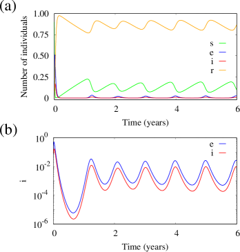
Figure 2: (a) SEIRS time series. (b) Magnification in log scale of the exposed (blue) and infected (red). We consider $\mu=0.02$, $\omega=2\pi$, $\alpha=37.35$, $\gamma=100$, $\delta=0.25$, $\beta_{1}=0.15$, and $\beta_{0}=800$.

The influences of $\beta_{0}$, $\delta$, $\beta_{1}$, and $\gamma$ in the dynamical system are exhibited in Figs. 3(a-d), respectively, by the bifurcation diagrams followed by the largest Lyapunov exponent ($\lambda_{1}$) [49]. The Lyapunov exponent is a tool to identify chaos [50]. A positive largest Lyapunov exponent ($\lambda_{1}>0$) corresponds to chaotic dynamics [51]. The bifurcations are constructed by the collection of the $i$ maxima points in the forward (red) and backward (blue) directions. The combination of distinct bifurcation in forward and backward directions comprises a hysteresis [36]. Also, the Lyapunov exponents are calculated in both directions. By considering these results, it is possible to locate ranges where two attractors coexist, both looking at the bifurcation and Lyapunov exponent. These regions are delimited by the black dotted square in the panels (a-d). The regions where this dynamical behaviour exists are called bistability. Systems with these dynamics are extremely sensitive to the initial state [31] and the presence of chaotic attractor in these systems is rare [30, 52].

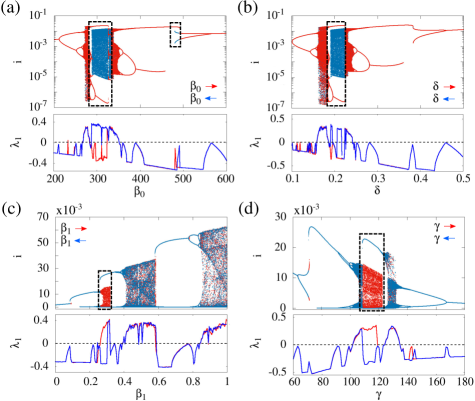
Figure 3: Bifurcations diagram and respective largest Lyapunov exponent ($\lambda_{1}$) for $\beta_{0}$ in the panel (a), for $\delta$ in the panel (b), for $\beta_{1}$ in the panel (c), and for $\gamma$ in the panel (d). The $i$ variable in the panels (a) and (b) is in log scale. We consider $\alpha=35.84$, $\mu=0.02$, $\omega=2\pi$, (a) $\gamma=100$, $\delta=0.20$, $\beta_{1}=0.28$, (b) $\gamma=100$, $\beta_{0}=300$, $\beta_{1}=0.28$, (c) $\gamma=100$, $\delta=0.25$, $\beta_{0}=270$, and (d) $\delta=0.25$, $\beta_{0}=300$, $\beta_{1}=0.28$.

The result in Fig. 3(a) shows bistability dynamics in the range $\beta_{0}\in[287,332]$ and $\beta_{0}\in[480,491]$. The bistability comprehends 14% of the $\beta_{0}$ range. However, for this parameter set, the dynamics is mostly periodic. The bifurcation for $\delta$ is very similar to the bifurcation for $\beta_{0}$, as shown in Fig. 3(b). For this parameter set, the bistability between periodic and chaotic attractor only exists in $\delta\in[0.19,0.22]$, which comprehends 7.5% of the $\delta$ range. Therefore, the time to lose immunity is relevant for the epidemic dynamics. Diseases with long time immunity, for example $>10$ years, or short time immunity, as for example $<3$ years, have periodic dynamics. Another analised parameter is the seasonality strength $\beta_{1}$, as displayed in Fig. 3(c). Our simulations show one region of bistability in $\beta_{1}\in[0.25,0.32]$ (7% of $\beta_{1}$ range) and most of the dynamics is sustained by chaotic attractors. Figure 3(d) exhibits the bifurcation as a function of $\gamma$, where one region of bistability in $\gamma\in[108,123]$ (19% of the $\gamma$ range), however, it is dominated by periodic behaviour. The $\omega$ parameter also is associated with the creation or annihilation of bistability dynamics, for example, for $\omega$ in the range 12 up to 30 months, the bistability is found. For values under 12 months the dynamics is periodic.

We observe that the parameters $\beta_{0}$, $\delta$, $\beta_{1}$, and $\gamma$ are relevant to understand the disease spread dynamics. However, we select the $\alpha$ parameter as the control parameter, once the bifurcation diagram for this parameter exhibits rich dynamic, it is possible to study the crisis and critical points, known as tipping points.

3 Bifurcation analysis

The latent period is an important variable in the dynamics of the epidemics [53] and is defined as $1/\alpha$ [3]. To understand the effects of $\alpha$ in the dynamical system (Eq. 5), we consider $\delta=0.25$, $\beta_{0}=270$, $\beta_{1}=0.28$, $\gamma=100$, and $\mu=b=0.02$, where the time unity is year. We choose $\alpha$ as the control due to the fact that the bistability and tipping points are more evident.

Figure 4 displays the bifurcation diagram (considering $i$ maximum) in the panel (a) and the largest Lyapunov exponent ($\lambda_{1}$) in the panel (b). Given an initial condition, the red point is the maximum value of $i$ in the forward $\alpha$ direction following the attractor, i.e., the initial condition for the current step is equal to the last step. The blue points are obtained in the backward $\alpha$ direction. In Fig. 4(a), the vertical lines ($T_{i}$) are the critical points that delimit the bifurcation, where $i=1,2,3,4$. The bistable chaotic-periodic occupies $\approx 70\%$ of the $\alpha$ range, while the coexistence between periodic-periodic $\approx 1\%$. The ranges $[T_{1},T_{2}]$ and $[T_{3},T_{4}]$ encompass the coexistence of $\lambda_{1}<0$ and $\lambda_{1}>0$ which confirms the bistability between periodic and chaotic attractors, as illustrated in Fig. 4(b).

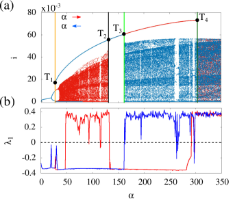
Figure 4: (a) Bifurcation diagram and (b) largest Lyapunov exponent. The red points and lines are forward and the blue points and lines are backward in the $\alpha$ parameter. We consider $T_{1}=27$, $T_{2}=130.88966$, $T_{3}=161.69990$, $T_{4}=303.88407$, $\delta=0.25$, $\beta_{0}=270$, $\beta_{1}=0.28$, and $\gamma=100$.

Due to the coexistence of two attractors, we compute two basins of attractions for different $\alpha$ values. For $\alpha=100$ in Figs. 5(a-c) and for $\alpha=200$ in Figs. 5(d-f). The colour scheme follows the colour of the attractor in Fig. 4. For $\alpha=100$, 43% of the basin formed by red points that evolve to the chaotic attractor is separately displayed in Fig. 5(b), while 57% of the basin is composed of blue points, which evolve to the periodic attractor as displayed in Fig. 5(c). The colour scale in Figs. 5(b), 5(c), 5(e) and 5(f) is $r_{0}$. The composition of the basin attraction is not preserved by $\alpha$ translation. However, in other ranges, for example $[T_{3},T_{4}]$, the shape of the basin attraction changes, as shown in Fig. 5(d), for $\alpha=200$. For this $\alpha$ value, 57% of the points evolve to the chaotic attractor. The basin for the chaotic attractor is shown in Fig. 5(e). The 43% of the remaining points evolve to the periodic attractor and are plotted in Fig. 5(f). The structure of this basin remains in the range $[T_{3},T_{4}]$. However, translations in $\alpha$ change the composition of the basin attraction, which decrease as a cubic function.

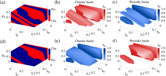
Figure 5: Basin attraction calculated for $\alpha=100$. In panel (a) there is the total basin attraction, in panel (b) the basin of chaotic attractor, and in panel (c) the periodic basin. In panels (d), (e), and (f), we calculate the basin for $\alpha=200$. We compute the chaotic and periodic basins in the panels (e) and (f), respectively.

The sudden change in the dynamical behaviour occurs at certain values of the control parameter, that are the critical points $T_{1}=27$, $T_{2}=130.88966$, $T_{3}=161.69990$, and $T_{4}=303.88407$. These events are called crises [54, 55] and are defined by the collision between a chaotic and a periodic attractor.

In the point $T_{1}$ occurs a rising of a bistable region by bifurcation. It starts by the existence of two different attractors, that are represented by blue and red branches. The bistability is formed by two periodic attractors until the point in which the red branch becomes chaotic by bifurcation. After that, the dynamics is sustained by the coexistence of periodic (blue) and chaotic (red) attractors until $T_{2}$.

The $3$-dimensional and $2$-dimensional projections of the attractors merging in $[T_{1},T_{2}]$ range are displayed in Figs. 6(a) and 6(b), respectively, for $\alpha=130$. The attractor shape is invariant by $\alpha\in[T_{1},T_{2}]$ translation. The attractors are constructed considering the stroboscopic map, that is a collection of the dynamical variables every $T=n\pi$, where $n=0,2,4,...$. Figures 6(c) and 6(d) display the $3$ and $2$-dimensional projections of the chaotic (blue points) and periodic (red points) in the range $[T_{3},T_{4}]$ for $\alpha=161.70276$. Figures 6(e) and 6(f) show the projections of the chaotic attractor for $\alpha>T_{4}$. In this regime, only chaotic attractor survives.

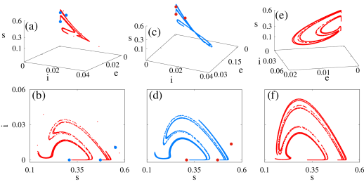
Figure 6: Coexistence of periodic and chaotic attractors. Three dimensional projection in the panels (a), (c), and (e). Bidimensional projection in the panels (b), (d), and (f). We consider $\alpha=130$ ((a) and (b)), $\alpha=161.70276$ ((c) and (d)), and $\alpha=303.88411$ ((e) and (f)). In the panels (a) and (b), the initial conditions for periodic is $(s_{0},e_{0},i_{0},r_{0})=(0.074,0.144,0.186,0.596)$ and for chaotic is $(s_{0},e_{0},i_{0},r_{0})=(0.075,0.145,0.185,0.595)$. For the panels (c) and (d), the initial conditions for periodic and chaotic are $(s_{0},e_{0},i_{0},r_{0})=(0.074,0.144,0.186,0.595)$ and $(s_{0},e_{0},i_{0},r_{0})=(0.060,0.100,0.110,0.730)$, respectively. For the panels (e) and (f) are $(s_{0},e_{0},i_{0},r_{0})=(0.074,0.144,0.186,0.596)$ and $(s_{0},e_{0},i_{0},r_{0})=(0.031,0,026,0,073,0,870)$. We consider $\mu=0.02$, $\omega=2\pi$, $\gamma=100$, $\delta=0.25$, $\beta_{1}=0.28$, and $\beta_{0}=270$.

Once crossed $T_{2}$, the bistability disappears and periodic behaviour prevails. In this point, the chaotic attractor collides with the periodic one by a saddle-point bifurcation. Around the crisis point, it is expected that the transient time tends to infinity. We calculate the average transient time $\langle\tau\rangle$ for $200$ initial conditions in the interval $[T_{2},130.89666]$, as displayed in Fig. 7 by red points. $\tau$ parameter represents the time to the chaotic attractor dynamics goes to the periodic one. The black curve is a Gaussian fit displayed by the equation

$$y=y_{0}+\frac{A}{\sigma\sqrt{\frac{\pi}{4\ln(2)}}}e^{-\frac{4\ln(2)(\langle\tau\rangle-\langle\tau\rangle_{\rm c})^{2}}{\sigma^{2}}}.$$ (6)

The $y_{0}$, $A$, $\sigma$ are parameters for the fitting. We observe the existence of a transient chaos around $T_{2}$, that has a distribution type Gaussian centered in $\langle\tau\rangle_{\rm c}=28\times 10^{4}$ years. In the range where transient chaos exists, the basin of attraction is composed of chaotic and periodic orbits. However, the initial conditions that evolve to chaotic attractor dissipate linearly and smoothly with the increase of the transient time.

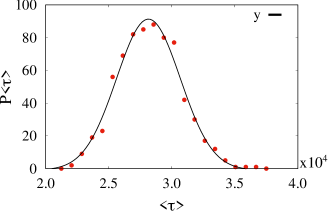
Figure 7: Distribution for the average transient time $\langle\tau\rangle$ in red points and range $[T_{2},130.89666]$. The average is calculated for $200$ samples of chaotic initial conditions. The black curve is a gaussian fit. We consider $\mu=0.02$, $\omega=2\pi$, $\gamma=100$, $\delta=0.25$, $\beta_{1}=0.28$, and $\beta_{0}=270$.

The point $T_{3}$ denotes the birth of a new bistable region. That happens by a transition from a periodic branch (blue) to a chaotic by a saddle point. In this transition also exists a transient chaos, which is displayed in Fig. 8 by the red points. The transient time in the range $[T_{3},161.70849]$ follows a binomial distribution, indicate by the continuous black lines $y_{1}$ and $y_{2}$, given by the log normal distribution

$$y=y_{0}+\frac{A}{\sqrt{2\pi}\sigma\tau}e^{-\frac{({\ln}(\langle\tau\rangle/\langle\tau\rangle_{\rm c}))^{2}}{2\sigma^{2}}},$$ (7)

where the first peak value is $\langle\tau\rangle=1.9\times 10^{4}$ years and the second one is $\langle\tau\rangle=3\times 10^{4}$ years. For $\alpha<T_{3}$ and close to $T_{3}$, there is transient chaos. The basin of attraction for the chaotic attractor is extinct linearly smooth with the increase of the transient.

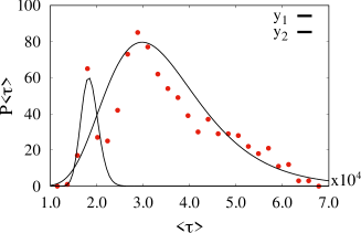
Figure 8: Distribution for the average transient time $\langle\tau\rangle$ in $[T_{3},161.70849]$ (red points). The black curve is the fit given by a log normal. The average is calculated for $200$ samples. We consider $\mu=0.02$, $\omega=2\pi$, $\gamma=100$, $\delta=0.25$, $\beta_{1}=0.28$, and $\beta_{0}=270$.

After crossing $T_{3}$, we observe a bistable regime that comprehends 40% of the $\alpha$ range. The bistability is sustained by the coexistence of periodic and chaotic attractors, as shown in Figs. 6(c) and 6(d). Crossing this bistable regime, we find the last crisis point ($T_{4}$). The transient time goes to infinity, following a decay $\propto x^{-1/2}$ as we move away from $T_{4}$. However, at this point, the transient is periodic. Figure 9 exhibits our result for $200$ periodic initial conditions. Differently from the two first cases, the transient goes to infinity for $T_{4}=\alpha_{c}$ and decays with $(\alpha-\alpha_{c})^{\gamma}$, where $\gamma=-0.5025\pm 0.0002$ and $\alpha>\alpha_{c}$, with this standard deviation value we can say that $\gamma=1/2$ that is the universality exponent for average duration of chaotic transients. The black line indicates the fit curve, that is given by $y=167.06(\alpha-\alpha_{c})^{-0.5025}$ with a correlation coefficient equal to $-0.9999549$. After this transient, the periodic points, in the phase space, coalesce in a chaotic attractor by a saddle-point. The basin of attraction in the crisis point is formed by 19% of the initial conditions that evolve to a periodic attractor. Increasing the transient time until $\tau=50800$, we verify an abrupt change and the fraction of periodic points goes to zero, discontinuously. The periodic transient persists until 1% above $\alpha_{c}$ calculated through $(\alpha-\alpha_{c})/\alpha_{c}$.

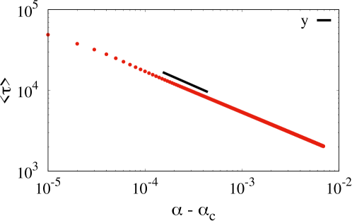
Figure 9: Average transient lifetime versus $\alpha-\alpha_{\rm c}$ in log scale for $200$ periodic initial conditions (red points). The black line indicates the fitting. We consider $\mu=0.02$, $\omega=2\pi$, $\gamma=100$, $\delta=0.25$, $\beta_{1}=0.28$, and $\beta_{0}=270$.

4 Tipping points

Tipping points mark changes in the system between alternative states [34]. It occurs when a threshold is crossed due to an external perturbation or by shift in the parameters of the system [56]. The transitions correspond to saddle-node or fold bifurcations [36]. Between two tipping points, the system is bistable, i.e., it can be found in one of two possible states [34].

In the seasonal disease context, the desired state is one in which the future outbreak is predictable. If the disease spread is predictable, based on the data from previous years, it is possible to construct more efficient control strategies and, consequently, decrease the number of infected individuals. The undesired state, on the other hand, is when the evolution of the disease spread is unpredictable. The unpredictability is associated with chaotic dynamics [45] and was studied by Scarpino and Petri [44]. However, until the moment, the mechanism behind the unpredictability is not satisfactorily explained by only the chaotic dynamics. In this work, we show that unpredictability is associated with bistable dynamics and has a tipping point.

Figure 10 exhibits the state variable as a function of the parameter control. We observe a state related to the predictable (green line) and another to the unpredictable (red line). The state variable can be the number of infected and the parameter control can be the $\alpha$ variable. With regard to the green curve, the control parameter is increased until tipping point $1$. At this point, the system reaches threshold $1$. Once crossed, the state variable evolves to the red branch, which represents the unpredictable state. If we start in the red branch and decrease the control parameter, then, after crossing threshold $2$, the system shifts to the green branch. Therefore, the state system can alternate between unpredictable and predictable due to parameter control. This situation illustrates what happens in points $T_{3}$ and $T_{4}$, as shown in Fig. 4.

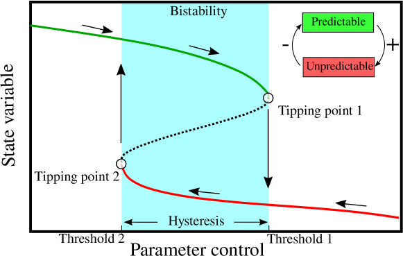
Figure 10: Representation of the tipping points between predictable (green branch) and unpredictable (red branch) states.

Firstly, we focus on the range $[T_{1},T_{2}]$ shown in Fig. 4. The system exhibits periodic behaviour for $\alpha<T_{1}$ and $\alpha>T_{2}$. However, it encompasses a bistable chaotic-periodic dynamics in the considered interval. In this region, the maximum number of infected individuals increases by 20 times from $T_{1}$ to $T_{2}$, however, in the boundary the attractors are periodic. The bistable region is interesting in terms of predictability, for the reason that small changes in the initial condition can leave the system from periodic to chaotic behaviours. In this region, the average probability of an initial condition evolving to the periodic behaviour is 49%. Therefore, with this measure, the predictability is uncertain in the interval $[T_{1},T_{2}]$.

In the range $[T_{3},T_{4}]$ are the tipping points illustrated in Fig. 10. Considering $T_{2}<\alpha<T_{3}$, all the initial conditions evolve to a periodic attractor, namely the dynamics is predictable. For example, based on the date of one year, it is possible to implement restrictions for the next year. Once crossed $T_{3}$, the dynamic becomes bistable. The range $[T_{3},T_{4}]$ is connected by the coexistence of chaotic and periodic dynamics. The probability of one initial condition evolving to a periodic attractor is displayed in Fig. 11. The probability distribution for $\alpha$ has a cubic decay as closer to $T_{4}$. The average is equal to 37% and we can affirm that diseases in $[T_{3},T_{4}]$ are preferably unpredictable. After crossing $T_{4}$, all the initial conditions evolve to the chaotic attractor and, as a consequence, the disease spread becomes unpredictable.

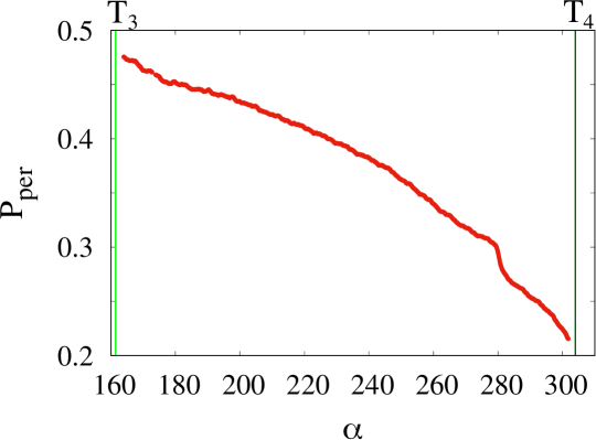
Figure 11: The probability of an initial condition evolves to the periodic attractor in the range $[T_{3},T_{4}]$ (vertical lines). We consider $\mu=0.02$, $\omega=2\pi$, $\gamma=100$, $\delta=0.25$, $\beta_{1}=0.28$, $\beta_{0}=270$.

5 Conclusions

In this work, we study a SEIR seasonal model with temporary immunity. The inclusion of temporary immunity greatly enriches the system dynamics. Our results show that the bistable dynamics depend on the control parameters. Thus, by varying $\alpha$, 70% of the range exhibits bistability, which is composed of chaotic and periodic attractors. Our results show the importance of all parameters in the spread dynamics, however, with the crisis present in the $\alpha$ bifurcation, it is possible to study tipping points phenomena. We explore a range that includes diseases with a latent period in order of days until hours [53].

We verify that the dynamics of the disease spread is chaotic for $\alpha\geq 300$. The diseases in this range have a latent period less than $1.2$ days. Only values in $0<\alpha\leq 30$ (very high values of $1/\alpha$ until $12$ days) and $130\leq\alpha\leq 161$ ($2.8$ until $2.2$ days) are periodic. Values above $\alpha>350$ are not considered.

The analysed range shows that the latent period is a crucial variable to understand the reason for the unpredictability of infectious diseases. This unpredictability was observed by Scarpino and Petri [44], however, the components of the unpredictability were unclear. Our results show that the unpredictability is closely associated with $\alpha$ due to bistable dynamics.

To finish this work, we answer the question provided in Introduction: the disease spread becomes unpredictable when the tipping point $T_{4}$ is crossed. Therefore, diseases with a short latent period, less than 30 hours, are always unpredictable.

Acknnowledgements

The authors thank Dr. E.S. Medeiros for discussions. The authors thank the financial support from the Brazilian Federal Agencies (CNPq), grants 407299/2018-1, 311168/2020-5, the São Paulo Research Foundation (FAPESP, Brazil) under grants 2018/03211-6, 2020/04624-2, 2022/05153-9, CAPES, Fundação Araucária. The authors thank 3D NeuroNets LLC. We thank 105 Group Science (www.105groupscience.com).

References

- [1] Anderson RM, May RM. (Eds.) Infectious Diseases of Humans: Dynamics and Control. Oxford: Oxford University Press; 1991.
- [2] Gabrick EC, Protachevicz PR, Batista AM, Iarosz KC, de Souza SLT, Almeida ACL, Szezech Jr. JD, Mugnaine M, Caldas IL. Effect of two vaccine doses in the SEIR epidemic model using a stochastic cellular automaton. Physica A 2022;597:127258.
- [3] Batista AM, de Souza SLT, Iarosz KC, Almeida ACL, Szezech Jr. JD, Gabrick EC, Mugnaine M, dos Santos GL, Caldas IL. Simulation of deterministic compartmental models for infectious diseases dynamics. Revista Brasileira de Ensino de Física 2021;43:e20210171.
- [4] Sharma N, Verma AK, Gupta AK. Spatial network based model forecasting transmission and control of COVID-19. Physica A 2021;581(1):126223.
- [5] Quan-Xing L, Zhen J. Cellular automata modelling of seirs. Chinese Physics 2005;14:1370.
- [6] Amaku M, Covas DT, Coutinho FAB, Azevedo RS, Massad E. Modelling the impact of delaying vaccination against SARS-CoV-2 assuming unlimited vaccine supply. Theoretical Biology and Medical Modelling 2021;18:1-14.
- [7] Carcione JM, Santos JE, Bagaini C, Ba J. A simulation of a COVID-19 epidemic based on a deterministic SEIR model. Frontiers in Public Health 2020;8:230.
- [8] Mugnaine M, Gabrick EC, Protachevicz PR, Iarosz KC, de Souza SLT, Almeida ACL, Batista AM, Caldas IL, Szezech Jr. JD, Viana RL. Control attenuation and temporary immunity in a cellular automata SEIR epidemic model. Chaos, Solitons and Fractals 2022;155:111784.
- [9] Abdelaziz MAM, Ismail AI, Abdullah FA, Mohd MH. Bifurcations and chaos in a discrete SI epidemic model with fractional order. Advances in Difference Equations 2018;2018:44.
- [10] Nakamura GM, Martinez AS. Hamiltonian dynamics of the SIS epidemic model with stochastic fluctuations. Scientific Report, 2019;9:15841.
- [11] Wei W, Xu W, Song Y, Liu J. Bifurcation and basin stability of an SIR epidemic model with limited medical resources and switching noise. Chaos, Solitons and Fractals 2021;152:111423.
- [12] Wang D, Zhao Y, Luo J, Leng H. Simplicial SIRS epidemic models with nonlinear incidence rates. Chaos 2021;31:053112.
- [13] de Souza SLT, Batista AM, Caldas IL, Iarosz KC, Szezech Jr. JD. Dynamics of epidemics: Impact of easing restrictions and control of infection spread. Chaos, Solitons and Fractals 2021;142:110431.
- [14] Cooper I, Mondal A, Antonopoulos CG. A SIR model assumption for the spread of COVID-19 in different communities. Chaos, Solitons and Fractals 2020;139:110057.
- [15] Aguiar M, Kooi B, Stollenwerk N. Epidemiology of Dengue Fever: A Model with Temporary Cross-Immunity and Possible Secondary Infection Shows Bifurcations and Chaotic Behaviour in Wide Parameter Regions. Mathematical Modelling of Natural Phenomena 2008:3;48-70.
- [16] Olsen LF, Schaffer WM. Chaos versus noisy periodicity: alternative hypotheses for childhood epidemics. Science 1990;249:499-503.
- [17] Tanaka G, Aihara K. Effects of seasonal variation patterns on recurrent outbreaks in epidemic models. Journal of Theoretical Biology 2013;317:87-95.
- [18] Galvis JA, Corzo CA, Machado G. Modelling and assessing additional transmission routes for porcine reproductive and respiratory syndrome virus: Vehicle movements and feed ingredients. Transboundary and Emerging Diseases 2022;1-12.
- [19] Moneim IA, Greenhalgh D. Use of a periodic vaccination strategy to control the spread of epidemics with seasonally varying contact rate. Mathematical Biosciences and Engineering 2005;2:591-611.
- [20] Buonomo B, Chitnis N, d’Onofrio A. Seasonality in epidemic models: a literature review. Ricerche di Matematica 2018;67:7-25.
- [21] Keeling MJ, Rohani P, Grenfell BT. Seasonally forced disease dynamics explored as switching between attractors. Physica D 2001;148:317–335.
- [22] London WP, Yorke JA. Recurrent outbreaks of measles, chikenpox and mumps: Seasonal variation in contact rates. American Journal of Epidemiology 1973;98:1-5.
- [23] Aguiar M, Ballesteros S, Kooi BW, Stollenwerk N. The role of seasonality and import in a minimalistic multi-strain dengue model capturing differences between primary and secondary infections: Complex dynamics and its implications for data analysis. Journal of Theoretical Biology 2011;289:181-196.
- [24] Stollenwerk N, Spaziani S, Mar J, Arrizabalaga IE, Knopoff D, Cusimano N, Anam V, Shrivastava A, Aguiar M. Seasonally Forced SIR Systems Applied to Respiratory Infectious Diseases, Bifurcations, and Chaos. Computational and Mathematical Methods 2022;2022:3556043.
- [25] He S, Peng Y, Sun K. SEIR modeling of the COVID-19 and its dynamics. Nonlinear Dynamics 2020;101:1667-1680.
- [26] Jones A, Strigul N. Is spread of COVID-19 a chaotic epidemic? Chaos, Solitons and Fractals 2021;142:110376.
- [27] Bilal S, Singh BK, Prasad A, Michael E. Effects of quasiperiodic forcing in epidemic models. Chaos 2016;26:093115.
- [28] Ventura PC, Aleta A, Rodrigues FA, Moreno Y. Epidemic spreading in populations of mobile agents with adaptive behavioral response. Chaos, Solitons and Fractals 2022;156:111849.
- [29] Cheng G, Gui R. Bistable chaotic family and its chaotic mechanism. Chaos, Solitons and Fractals 2022;162:112407.
- [30] Feudel U, Grebogi C. Multistable and the control of complexity. Chaos 1997;7:597.
- [31] Feudel U. Complex dynamics in multistable systems. International Journal of Bifurcation and Chaos 2008;18:1607-1626.
- [32] Lenton TM. Early warning of climate tipping points. Nature Climate Change, 2011;1:201-209.
- [33] Scheffer M, Carpenter SR, Dakos V, van Nes EH. Generic Indicators of Ecological Resilience: Inferring the Chance of a Critical Transition. Annual Review of Ecology, Evolution, and Systematics 2015;46:145-167.
- [34] Dakos V, Matthews B, Hendry AP, Levine J, Loeuille N, Norberg J, Nosil P, Scheffer M, De Meester L. Ecosystem tipping points in an evolving world. Nature Ecology & Evolution 2019;3:355-362.
- [35] Wright RJ, Hanson HA. A tipping point in cancer epidemiology: embracing a life course exposomic framework. Trends in Cancer 2022;8:280-282.
- [36] Medeiros ES, Caldas IL, Baptista MS, Feudel U. Trapping phenomenon attenuates the consequences of tipping points for limit cycles. Scientific Reports 2017;7:42351.
- [37] Ansari S, Anvari M, Pfeffer O, Molkentin N, Moosavi MR, Hellmann F, Heitzig J, Kurths J. Moving the epidemic tipping point through topologically targeted social distancing. Eur. Phys. J. Spec. Top. 2021;230:3273-3280.
- [38] O’Regan SM, O’Dea EB, Rohani P, Drake JM. Transient indicators of tipping points in infectious diseases. Journal of the Royal Society Interface 2020;17:0200094.
- [39] Francomano E, Hilker FM, Paliaga M, Venturino E. Separatrix reconstruction to identify tipping points in an eco-epidemiological model. Applied Mathematics and Computation 2018;318:80-91.
- [40] Meng Y, Grebogi C, Lai YC. Noise-enabled species recovery in the aftermath of a tipping point. Physical Review E 2020;101:012206.
- [41] Meng Y, Grebogi C. Control of tipping points in stochastic mutualistic complex networks. Chaos 2021;31:023118.
- [42] Grebogi C, Ott E, Yorke JA. Super persistent chaotic transients. Ergodic Theory and Dynamical Systems 1985;5:341-372.
- [43] Hastings A, Abbott KC, Cuddington K, Francis TB, Lai YC, Morozov A, Petrovskii S, Zeeman ML. Effects of stochasticity on the length and behaviour of ecological transients. Journal of the Royal Society Interface 2021;18:20210257.
- [44] Scarpino SV, Petri G. On the predictability of infectious disease outbreaks. Nature Communications 2019;10:898.
- [45] Stollenwerk N, Aguiar M, Ballesteros S, Boto J, Kooi B, Mateus L. Dynamic noise, chaos and parameter estimation in population biology. Interface Focus 2012;2:156-169.
- [46] Bai Z, Zhou Y. Global dynamics of an SEIRS epidemic model with periodic vaccination and seasonal contact rate. Nonlinear Analysis: Real World Applications 2012;13:1060-1068.
- [47] Yi N, Zhang Q, Mao K, Yang D, Li Q. Analysis and control of an SEIR epidemic system with nonlinear transmission rate. Mathematical and Computer Modelling 2009;50:1498-1513.
- [48] Keeling MJ, Rohani P. Modeling Infectious Diseases in humans and animals. Princeton: Princeton University Press; 2008.
- [49] Wolf A, Swift JB, Swinney HL, Vastano J. Determining Lyapunov exponents from a time series. Physica D: Nonlinear Phenomena 1985;16(3):285-317.
- [50] Tél T, Gruiz M. Chaotic Dynamics: An introduction based on Classical Mechanics. Cambridge: Cambridge University Press; 2006.
- [51] Alligood KT, Sauer T, Yorke JA. Chaos: an introduction to dynamics systems. New York: Springer; 1996.
- [52] Feudel U, Grebogi C. Why are chaotic attractors rare in multistable systems? Physical Review Letters 2003;91:134102.
- [53] Lessler J, Reich NG, Brookmeyer R, Perl TM, Nelson KE, Cummings DAT. Incubation periods of acute respiratory viral infections: a systematic review. Lancet 2009;9:291-300.
- [54] Grebogi C, Ott E, Yorke JA. Chaotic attractor in crisis. Physical Review Letters 1982;48:1507.
- [55] Grebogi C, Ott E, Yorke JA. Crises, sudden changes in chaotic attractors, and transient chaos. Physica D 1983;7:181-200.
- [56] Van Nes EH, Arani BMS, Staal A, van der Bolt B, Flores BM, Bathiany S, Scheffer M. What do you mean, “Tipping Point”? Trends in Ecology & Evolution 2016;31:902-904.