Self-training via Metric Learning for Source-Free Domain Adaptation of Semantic Segmentation

Abstract

Unsupervised source-free domain adaptation methods aim to train a model to be used in the target domain utilizing the pretrained source-domain model and unlabeled target-domain data, where the source data may not be accessible due to intellectual property or privacy issues. These methods frequently utilize self-training with pseudo-labeling thresholded by prediction confidence. In a source-free scenario, only supervision comes from target data, and thresholding limits the contribution of the self-training. In this study, we utilize self-training with a mean-teacher approach. The student network is trained with all predictions of the teacher network. Instead of thresholding the predictions, the gradients calculated from the pseudo-labels are weighted based on the reliability of the teacher’s predictions. We propose a novel method that uses proxy-based metric learning to estimate reliability. We train a metric network on the encoder features of the teacher network. Since the teacher is updated with the moving average, the encoder feature space is slowly changing. Therefore, the metric network can be updated in training time, which enables end-to-end training. We also propose a metric-based online ClassMix method to augment the input of the student network where the patches to be mixed are decided based on the metric reliability. We evaluated our method in synthetic-to-real and cross-city scenarios. The benchmarks show that our method significantly outperforms the existing state-of-the-art methods.

I Introduction

Thanks to advances in deep learning, computer vision has made significant progress in recent years. Deep learning networks trained in a supervised manner achieve high performance even in challenging tasks that require dense prediction, such as semantic segmentation [1, 2, 3, 4]. However, preparing a large dataset with dense labeling is very laborious and expensive [5]. An approach to decrease the workforce may be using public real [6, 5, 7] or synthetic datasets [8, 9]. However, deep learning approaches assume the IID distribution of train and test sets. Since the marginal distribution of the source domain and target domain are different, the trained model suffers from performance degradation when the model is evaluated on the target data. This problem is called the domain gap.

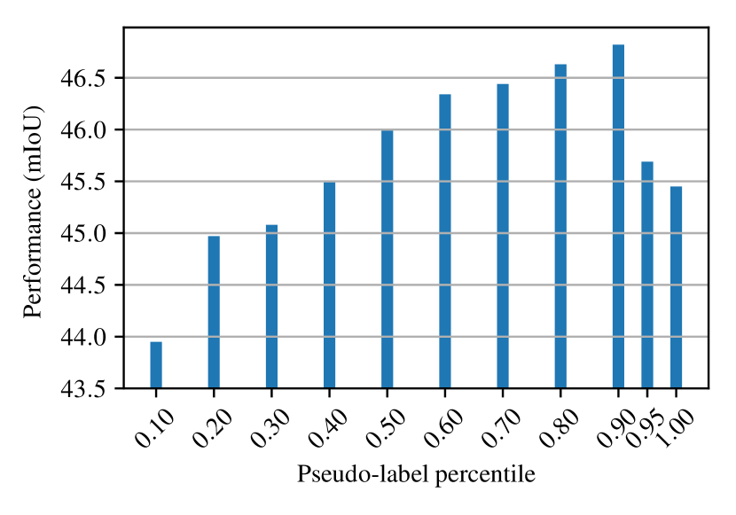
Figure 1: Segmentation performance of the self-training when different percentile of the predictions are used as pseudo-labels

Recently, domain adaptation methods have been proposed to mitigate domain gap [10, 11, 12, 13, 14, 15, 16]. Such methods use labeled source domain data and unlabeled target domain data together when training the model. However, the source domain data may not be accessible due to intellectual property (IP) or privacy issues in some applications like medical imaging or autonomous driving. A possible solution to this problem is using the model trained in the source domain instead of data. The problem setting of using the source model and target data in order to decrease the domain gap is called source-free domain adaptation. In this study, we propose a method for source-free domain adaptation of semantic segmentation called Self-Training via Metric learning (STvM).

Self-training is widely used in both classical domain adaptation and source-free domain adaptation. Self-training is a training strategy in deep learning where the model fits the pseudo-labels predicted by itself. Most methods use prediction filtering to decide pseudo-labels [17, 18, 19, 20]. In source-free domain adaptation, the only supervision comes from the target dataset since the source dataset does not exist. Therefore, the predictions of the target images should be exploited in training as much as possible. However, using all predictions is not a good strategy since false predictions give wrong supervision to the training, which decreases performance, as shown in Figure 1. Therefore, instead of filtering them, we scale the gradients based on the reliability of the prediction.

Neural networks may make overconfident false predictions for data far away from training sets, such as out-of-distribution images [21]. The images belonging to the target dataset are out-of-distribution images for the model trained in the source domain. Therefore, a good measure that is valid in the target domain is needed. To this end, we propose a novel reliability measure defined in the target domain using pixel-level proxy-based metric learning. A network called a metric network is trained to predict a distance metric for each input image pixel, where pixels belonging to the same class are close to each other and far away from the pixels from the other classes. We adopt the proxy-based metric learning approach, where a proxy feature vector is trained for each class. These features can be considered as class prototypes. The distance between the pixel feature and the proxy feature of the predicted class is used to calculate reliability.

Recently, the ClassMix [22] data augmentation technique showed its effectiveness in semi-supervised semantic segmentation tasks. It cuts half of the classes from one image and pastes on another by also transferring class labels. However, the data is unlabeled in a source-free domain adaptation setting which prevents using ClassMix directly. Therefore, we propose a metric-based online ClassMix method. In training time, we store a fixed-size patch buffer for each class separately. If the average metric distance of a patch is lower than a threshold, it is added to the patch buffer and used for mixing in training time.

In summary, our contributions are as follows:

• We propose a novel reliability metric that is directly learned in the target domain using a proxy-based metric learning approach.

• Instead of filtering the prediction to decide pseudo-labels, we use all predictions in self-training and scale the gradients based on the reliability metric.

• We propose a metric-based online ClassMix method to augment the input image.

• STvM significantly outperforms state-of-the-art methods on GTA5-to-CityScapes, SYNTHIA-to-CityScapes, and NTHU datasets.

II Related works

Domain adaptation.

Domain adaptation is a widely studied topic, especially for image classification [23] and semantic segmentation [24]. Adversarial learning [25, 26, 12, 27, 28, 29, 20] and self-training [30, 31, 19, 14, 32, 33, 18, 17] approaches are commonly utilized in semantic segmentation. Adversarial methods enforce the feature space of the source and target space to be aligned inspired by the GAN framework [34], where the source and the target domains are discriminated instead of real and fake samples. Adversarial learning is applied in image and feature levels. Some methods exploit the adversarial approach to the low-dimensional output space to facilitate adversarial learning. Self-training methods use confident predictions as pseudo-labels, obtained by filtering-out noisy samples or applying constraints, and train in a supervised manner with them.

Source-free domain adaptation.

Source-free domain adaptation applies domain adaptation using only the trained source model instead of the source data as well as unlabeled target data, where the source data cannot be freely shared due to Intellectual Property of privacy concerns. The task is recently introduced by two works [35, 36] concurrently. URMA [35] enforces confident predictions under the feature noise. It uses multiple decoders and introduces feature noise with dropout. The noise resilience is satisfied by uncertainty loss which is the squared difference of the decoder outputs. The training stability is improved with entropy minimization and self-training with threshold-based pseudo-labeling. SFDA [36] introduces a data-free knowledge distillation approach. It generates source domain synthetic images that preserve semantic information using batch-norm statistics of the model and dual-attention mechanism. They also use a self-supervision module to improve performance. GtA [37] categorized the SF-UDA methods as a vendor and client-side strategies, where vendor-side strategies focus on the improving source model for better adaptation. They focus on improving the vendor side performance and propose multiple augmentation techniques to train different source models using the leave-one-out technique on the vendor side.

Considering that it may not be possible to train the model on the vendor-side in source-free scenario, we propose a client-side source free domain adaptation method like SFDA and URMA, in which the source model is used as-is.

Metric learning.

Deep metric learning (DML) is an approach to establish a distance metric between data to measure similarity. It learns an embedding space where similar examples are close to each other, and different examples are far away. It is a widely studied topic in computer vision that has various applications such as image retrieval [38], clustering [39], person re-identification [40] and face recognition [41]. In the unsupervised domain adaptation literature, metric learning is mostly utilized in the image classification task. The features of the semantically similar samples from both source and target domain are aligned to mitigate the domain gap [42, 43, 44, 45]. Commonly, the similarity metric between images or patches is trained in deep metric learning. With a different perspective, Chen et al. [46] utilize pixel-wise deep metric learning for interactive object segmentation, where they model the task as an image retrieval problem. DML approaches are categorized into two classes based on the loss functions, namely pair-based and proxy-based methods. While pair-based loss functions [47, 48, 49, 50] exploit the data-to-data relations, the proxy-based loss functions [38, 51, 52, 53] exploit data-to-proxy relations. Generally, the number of proxies is substantially smaller than training data. Therefore, proxy-based methods converge faster, and the training complexity is smaller than pair-based methods. They are also more robust to label noise and outliers [54].

In STvM, we propose a proxy-based pixel-wise metric learning to estimate pseudo-label reliability, trained by limited and possibly noisy pseudo-labels.

Mixing.

Mixing is an augmentation technique that combines pixels of two training images to create highly perturbed samples. It has been utilized in classification [55, 56, 57] and semantic segmentation [58, 22]. Especially in semi-supervised learning of semantic segmentation, mixing methods, such as CutMix [56] and ClassMix [22], achieved promising results. While the former cut rectangular regions from one image and paste them onto another, the latter use a binary mask belonging to some classes to cut. DACS [59] adapts ClassMix [22] for domain adaptation by mixing across domains.

III Proposed method

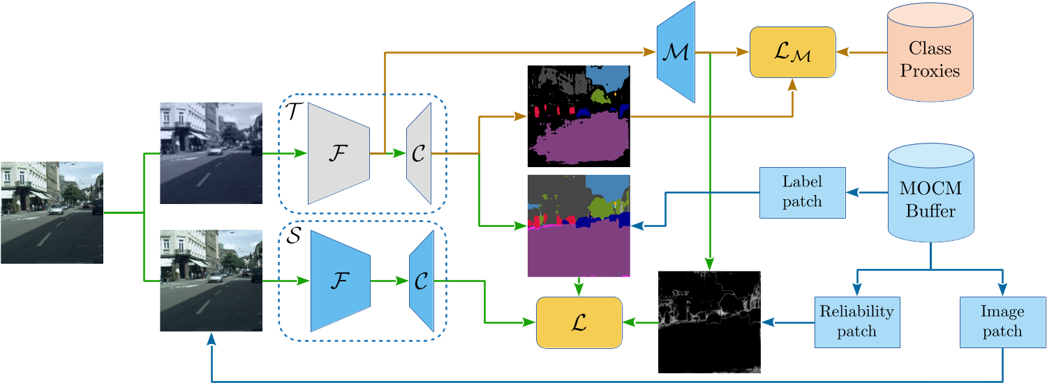
Figure 2: STvM comprises three networks, namely teacher, student, and metric network, represented as $\mathcal{T}$, $\mathcal{S}$, and $\mathcal{M}$, respectively. The teacher and the student network use the same segmentation network architecture. Each segmentation network is composed of feature extractor $\mathcal{F}$ and classifier $\mathcal{C}$. The metric network has the same architecture as $\mathcal{C}$, trained to learn metric feature space. Inspired by the mean-teacher approach, the student network is trained with a backpropagation algorithm. On the other hand, the parameters of the teacher model are updated with the moving average of the parameters of the student model. The metric network $\mathcal{M}$ and proxy features are also trained with a backpropagation algorithm.

In this section, we present our self-training via metric learning (STvM) approach for unsupervised source-free domain adaptation problem that we used for semantic segmentation. The source-free domain adaptation setting is composed of the following components. Let $\mathcal{D}_{S}$ is a labeled source dataset composed of source domain images $x_{S}$ and corresponding pixel-wise labels $y_{S}$, $\mathcal{D}_{S}=\{(x_{S}^{i},y_{S}^{i})\}_{i=1}^{N_{S}}$ where $N_{S}$ is the number of samples in $\mathcal{D}_{S}$. It is assumed that the source model is trained with $\mathcal{D}_{S}$ in a supervised manner so that it performs well in the source domain. Let $\mathcal{D}_{T}$ is an unlabeled target dataset composed of target domain images, $\mathcal{D}_{T}=\{(x_{T}^{i})\}_{i=1}^{N_{T}}$ where $N_{T}$ is the number of samples in $\mathcal{D}_{T}$. The source-free domain adaptation trains a model using only the pretrained source domain model and an unlabeled target dataset $\mathcal{D}_{T}$. Our method utilizes the mean teacher model. It consists of two segmentation networks called the teacher network $\mathcal{T}$ and the student network $\mathcal{S}$. Both networks are initialized with the source model enabling knowledge transfer from the source domain to the target domain. They are trained with target dataset $\mathcal{D}_{T}$ in an unsupervised manner.

III-A Framework overview

The proposed method is illustrated in the Figure 2. We utilize the mean-teacher approach to train a segmentation model. There are two data paths in STvM: One belongs to the teacher and metric networks, and the other belongs to the student.

The teacher data path is responsible for training the metric network, generating the pseudo-labels and the reliability map. An image belonging to the target dataset is fed to the teacher network. The predictions of the teacher model are used as pseudo-labels. In addition to that, the features generated by the feature extractor of the teacher network are fed to the metric network to form metric features for each pixel of the input image. The distance between the proxy feature of the predicted class and the metric feature is used as a class similarity map. A proxy feature is a vector representing the class distribution in metric space. The class similarity map is converted to a reliability score using the reverse sigmoid function. The metric network is trained with a proxy-based metric learning approach using the highly confident predictions of the teacher network.

The student data path is responsible for the training of the student network using pseudo-labels and reliability scores. Firstly, A photometric augmentation is applied to the input image, then Metric-based Online ClassMix (MOCM) augmentation is applied to the input image, the pseudo-labels, and the reliability map. The patches that are used in MOCM are determined and stored to the patch buffer in training time based on the metric similarity. The online patch update approach enables end-to-end training of the student model. The student model is trained with a classical pixel-wise cross-entropy loss function. However, the pixel-wise loss is multiplied with a reliability score to scale gradients which suppress erroneous pseudo-labels and allow under-confident accurate predictions to contribute to training.

III-B Mean teacher with noisy student

The mean teacher method constitutes two networks called the teacher and the student networks [60]. The parameters of the teacher network are updated by moving average of the student network parameters where the student network is updated with backpropagation. The mean teacher approach can be integrated with the self-training concept by generating the pseudo-labels from the teacher network and training the student network with these pseudo-labels. In order to obtain pseudo-labels as accurately as possible, we do not apply augmentation to the input of the student network. The continuous update of the teacher network enables gradually improved pseudo-labels during training. Xie et al. [61] showed that deliberately adding noise to the student model leads to a better teacher model. Following the same principle, we applied an input noise using photometric augmentation and MOCM.

For the segmentation task, the teacher network $\mathcal{T}$ takes an image $x_{T}^{i}\in X_{T}\subset\mathbb{R}^{H\times W\times 3}$ and generate a class probability distribution $p_{T}\in P_{T}\subset\mathbb{R}^{H\times W\times C}$ for each pixel, where $H$, $W$, and $C$ correspond to the image height, the image width and the number of classes, respectively. The pseudo-label map $\tilde{y}\in\mathbb{R}^{H\times W\times C}$ is a one-hot vector for each pixel, where the channel corresponding to the maximum prediction confidence is one and the others are zero.

The pixel-wise cross-entropy loss is a widely used criterion in semantic segmentation tasks. We adapted the cross-entropy loss to train the student network. Different from the existing methods, all pseudo-labels are taken into account to train the student network. However, the gradients computed by pseudo-labels are scaled based on the label’s reliability. We multiply pixel-wise loss values with the gradient scaling factor using Hadamard multiplication to scale the gradients. The gradient scaling factor $w^{(w,h)}$ is a real-valued map taking values between 0 and 1, and it is calculated based on the reliability metric, explained in section III-C in detail.

III-C Reliability metric learning

The gradient scaling factor ($w$) plays an important role in the training of the student model. It has a strong effect on the parameters of the student model since it manipulates the gradients. In addition to that, the student model parameters directly affect the teacher model’s performance and consequently the quality of the pseudo-labels. Therefore, It is essential to estimate a good reliability metric in the target domain to calculate the scaling factor. To this end, we proposed a novel reliability metric predicted by the metric network $\mathcal{M}$. The metric network utilizes the same architecture with the classifier $\mathcal{C}$ of the segmentation network. It takes the features of the feature extractor network $\mathcal{F}$ of the teacher network $\mathcal{T}$, and predicts a pixel-wise metric feature $f\in\mathbb{R}^{H\times W\times N_{f}}$, corresponding one metric feature for each input image pixel. The metric network $\mathcal{M}$ learns a transformation from the segmentation feature space to the metric feature space, where the features of the pixels belonging to the same class are pulled together, and those of the pixels belonging to different classes are pushed away.

The metric learning methods commonly use two different relations to train the model, namely pair-based and proxy-based relations. The pair-based methods use data-to-data similarity to train the network, whereas the proxy-based network uses proxy-to-data similarity. We exploit a proxy based relation in our study. The proxy feature $f_{p}\in\mathbb{R}^{N_{f}}$ is a vector that represents the distribution of a class of data points. We assign a different proxy feature to each segmentation class since we want to estimate how much the data point is associated with the predicted class. The proxy features are defined as a trainable parameter just as the metric learning network parameters, and it is trained concurrently with the metric network parameters.

Metric learning is a supervised learning method that requires class labels to be trained. Since the proxy-based method is known to be trained with a small number of samples [38, 51], we use a small subset of the predictions of the teacher network with high confidence values to train the metric network. This subset is called the metric pseudo-labels, and they are selected with class balanced thresholding strategy.

$$\tilde{y}_{M}^{h,w,c}=\begin{cases}\begin{array}[]{c}1\\ 0\end{array}&\begin{array}[]{c}p_{T}^{h,w,c}=\max(p_{T}^{h,w})>\tau_{c}\\ elsewhere\end{array}\end{cases}.$$ (1)

Threshold values ($\tau$) are varied for each class. Class-balanced thresholding strategy [17] selects a certain percentile ($q_{M}$) of the prediction confidences. We choose a low percentile value to obtain highly confident predictions. Threshold values are calculated in training time with the moving average of the percentile of the prediction of the current frame.

One successful approach in proxy-based metric learning is to use neighborhood component analysis (NCA) in training, where the samples are compared against proxies. The proxy features and the metric network parameters are updated concurrently to attract the feature of a sample to the corresponding proxy feature and repel from the other proxy features. We apply a similar approach to train the metric network and proxy features. A temperature scaling is an effective method. Teh et al. [51] show that using small $T$ values refine decision boundaries and help classify samples better. Motivated by these, we utilize NCA with temperature scaling. We select an equal number of samples in each class in $\tilde{y}_{M}^{h,w,c}$ to ensure balanced training. The metric network is optimized the following loss function:

$$\mathcal{L}_{M}=\sum_{h,w}\left[-\log\left(\frac{\exp(-d(f^{h,w},f_{p})*\frac{1}{T})}{\sum_{c}\exp(-d(f^{h,w},f_{p_{c}})*\frac{1}{T})}\right)\right],$$ (2)

where $T$ is a temperature and $d(x,y)$ is a normalized squared L2-Norm:

$$d(x,y)=\sum_{i}\left(\frac{x_{i}}{\left\lVert x\right\rVert}-\frac{y_{i}}{\left\lVert y\right\rVert}\right)^{2}$$ (3)

The same distance function is used in both training the metric network and calculating the reliability score, which is used as the gradient scaling factor. The smaller the distance gets, the more similar to the corresponding class it becomes. In order to calculate the similarity, we first feed the features of the feature extractor network of the teacher model to the metric network. The metric network outputs a metric feature for each pixel of the input image of the teacher network. Then we generate the similarity map by calculating the distance between the metric features and the proxy feature of the class predicted by the teacher network. We use a reverse sigmoid function to transform similarity to the reliability, where $\alpha$ is sharpness constant, and $\beta$ is offset of the sigmoid function:

$$w^{(h,w)}=\frac{1}{1+e^{-\alpha*(\beta-d(f^{h,w},\hat{f_{p}}))}}$$ (4)

III-D Metric-based online ClassMix

The noise injection to the input of the student model leads to a better generalization for both the student and teacher model [61]. Data augmentation with photometric noise is a common approach in computer vision applications. Another effective augmentation technique for classification and semantic segmentation is the mixing method. The mixing methods combine pixels from two training images to create a hıghly perturbed sample. ClassMix algorithm [22] is a mixing data augmentation method that cuts half of the classes in the predicted image and pastes on the other image.

The straightforward integration of the ClassMix method would be cutting half of the classes based on the prediction of the teacher network and pasting on the input of the student network. However, such an approach would not be beneficial since the input of the student model is the same as of the teacher model’s input except for the photometric noise. We propose a metric-based Online ClassMix (MOCM) method that stores reliable patches in training time using metric distance and uses these patches to mix the input data to overcome this problem.

We keep a patch buffer for each class separately. The patch buffers are fixed-sized and employ a first-in-first-out scheme that decreases the memory requirement and ensures that always up-to-date patches are stored in the buffer. Unlike the standard ClassMix approach, we use distances predicted by the metric network to proxy features to select patches. If the average distance of the metric features to the corresponding class proxy ($f_{p}^{c}$) of a patch is smaller than a threshold ($\tau_{MOCM}$), the patch is added to the buffer of the class $c$. The image, pseudo-label, and reliability map patch tuple is stored in the buffer since the mixing operation occurs in both image and label space.

To utilize the stored patches, we first apply a photometric noise to the input image, then apply the proposed MOCM method. We sample one patch from each $N_{MOCM}$ classes randomly and paste them onto the image ($x_{CM}$), pseudo-label ($\tilde{y}_{CM}$), and reliability map ($w_{MOCM}$). The training of the student network is performed by the stochastic gradient descent in order to minimize the following loss function:

$$\mathcal{L}=\frac{1}{H\times W}\sum\Biggl{[}\Biggl{(} -\sum_{c}\tilde{y}_{MOCM}^{h,w,c}\times\log(T(x_{MOCM})^{h,w,c})\Biggr{)}$$ (5)

$$\circ w_{MOCM}^{h,w}\Biggr{]}.$$

IV Experiments

TABLE I: Comparison with state-of-the-art on GTAV-to-CityScapes in terms of per-class IoUs and mIoU (%). SF represents if the method is in the source-free setting.

Method	Network	SF	Road	Sidewalk	Building	Wall	Fence	Pole	Light	Sign	Veg.	Terrain	Sky	Person	Rider	Car	Truck	Bus	Train	Mbike	Bicycle	mIoU
AdvEnt [62]	DeepLabV2	✗	89.4	33.1	81.0	26.6	26.8	27.2	33.5	24.7	83.9	36.7	78.8	58.7	30.5	84.8	38.5	44.5	1.7	31.6	32.4	45.5
Intra-domain [14]		✗	90.6	37.1	82.6	30.1	19.1	29.5	32.4	20.6	85.7	40.5	79.7	58.7	31.1	86.3	31.5	48.3	0.0	30.2	35.8	45.8
MaxSquare [30]		✗	89.4	43.0	82.1	30.5	21.3	30.3	34.7	24.0	85.3	39.4	78.2	63.0	22.9	84.6	36.4	43.0	5.5	34.7	33.5	46.4
LSE + FL [63]		✗	90.2	40.0	83.5	31.9	26.4	32.6	38.7	37.5	81.0	34.2	84.6	61.6	33.4	82.5	32.8	45.9	6.7	29.1	30.6	47.5
BDL [20]		✗	91.0	44.7	84.2	34.6	27.6	30.2	36.0	36.0	85.0	43.6	83.0	58.6	31.6	83.3	35.3	49.7	3.3	28.8	35.6	48.5
Stuff and Things [64]		✗	90.6	44.7	84.8	34.3	28.7	31.6	35.0	37.6	84.7	43.3	85.3	57.0	31.5	83.8	42.6	48.5	1.9	30.4	39.0	49.2
Texture Invariant [65]		✗	92.9	55.0	85.3	34.2	31.1	34.9	40.7	34.0	85.2	40.1	87.1	61.0	31.1	82.5	32.3	42.9	0.3	36.4	46.1	50.2
FDA [66]		✗	92.5	53.3	82.4	26.5	27.6	36.4	40.6	38.9	82.3	39.8	78.0	62.6	34.4	84.9	34.1	53.1	16.9	27.7	46.4	50.4
DMLC [67]		✗	92.8	58.1	86.2	39.7	33.1	36.3	42.0	38.6	85.5	37.8	87.6	62.8	31.7	84.8	35.7	50.3	2.0	36.8	48.0	52.1
URMA [35]		✓	92.3	55.2	81.6	30.8	18.8	37.1	17.7	12.1	84.2	35.9	83.8	57.7	24.1	81.7	27.5	44.3	6.9	24.1	40.4	45.1
SRDA [68]		✓	90.5	47.1	82.8	32.8	28.0	29.9	35.9	34.8	83.3	39.7	76.1	57.3	23.6	79.5	30.7	40.2	0.0	26.6	30.9	45.8
STvM (w/o MST)		✓	91.4	52.9	87.3	41.5	33.3	35.9	40.8	48.5	87.3	49.2	87.4	62.2	9.3	87.1	45.5	58.7	0.0	47.4	59.8	54.0
STvM (w/ MST)		✓	92.1	55.1	87.6	45.5	33.3	36.1	41.8	48.6	87.9	51.1	87.6	63.2	8.6	87.0	47.8	59.8	0.0	50.1	60.4	54.9
MinEnt [62]	DeepLabV3	✗	80.2	31.9	81.4	25.1	20.8	24.6	30.2	17.5	83.2	18.0	76.2	55.2	24.6	75.5	33.2	31.2	4.4	27.4	22.9	40.2
AdaptSegNet [12]		✗	81.6	26.6	79.5	20.7	20.5	23.7	29.9	22.6	81.6	26.7	81.2	52.4	20.2	79.1	36.0	28.8	7.5	24.7	26.2	40.5
CBST [17]		✗	84.8	41.5	80.4	19.5	22.4	24.7	30.2	20.4	83.5	29.6	82.3	54.7	25.3	79.2	34.5	32.3	6.8	29.0	34.9	42.9
MaxSquare [30]		✗	85.8	33.6	82.4	25.3	25.0	26.5	33.3	18.7	83.2	32.9	79.8	57.8	22.2	81.0	32.1	32.6	5.2	29.8	32.4	43.1
SFDA [36]		✓	84.2	39.2	82.7	27.5	22.1	25.9	31.1	21.9	82.4	30.5	85.3	58.7	22.1	80.0	33.1	31.5	3.6	27.8	30.6	43.2
STvM (w/o MST)		✓	90.3	50.2	87.4	37.9	33.0	35.8	45.2	48.5	85.7	44.1	86.1	62.4	29.8	84.3	30.2	50.0	0.6	7.4	0.0	47.8
STvM (w/ MST)		✓	90.8	50.7	87.7	40.9	32.0	36.1	47.2	48.6	85.9	43.3	87.0	62.9	31.5	85.2	34.6	54.0	0.6	7.8	0.0	48.8

IV-A Datasets

We demonstrate the performance of STvM on three different source-to-target adaptation scenarios which are GTA5-to-Cityscapes, Synthia-to-Cityscapes, and Cityscapes-to-NTHU Cross-City.

The Cityscapes [5] dataset consists of 5000 real-world street-view images captured in 50 different cities. The images have high-quality pixel-level annotations with a resolution of 2048 x 1024. They are annotated with 19 semantic labels for semantic segmentation. The Cityscapes is split into training, validation, and test sets containing 2975, 500, and 1525 images, respectively. The methods are evaluated on the validation set following the standard setting used in the previous domain adaptation studies. The GTA5 [8] is a synthetic dataset where images and labels are automatically grabbed from Grand Theft Auto V video game. It consists of 24,966 synthetic images with the size of 1914 x 1052. They have pixel-level annotations of 33 categories. The 19 classes compatible with the Cityscapes are used in the experiments. The Synthia [9] is also a synthetic dataset. It is composed of urban scene images with pixel-level annotations. The commonly used SYNTHIA-RAND-CITYSCAPES subset contains 9,400 images with a resolution of 1280 x 760. The dataset has 16 shared categories with the Cityscapes dataset. Cross-City [7] is a real-world dataset. The images are recorded in four cities, which are Rome, Rio, Taipei, and Tokyo. The dataset has 3200 unlabeled images as a training set and 100 labeled images for the test set with the size of 2048 x 1024. Cross-City has 13 shared classes with the Cityscapes dataset.

IV-B Implementation details

We utilize two different segmentation networks to make a fair comparison with the previous unsupervised source-free domain adaptation for semantic segmentation methods. One is DeepLabV2 [2] with the ResNet-101 backbone, and the other is the DeepLabV3 [1] network with the ResNet–50 backbone. The same architecture is used for both the teacher ($\mathcal{T}$) and the student ($\mathcal{S}$) networks. ResNet-101 and ResNet-50 are used as feature extractor. The same architecture is used for the classifier ($\mathcal{C}$) and metric ($\mathcal{M}$) networks, which is the corresponding ASPP module of DeepLabV2 and DeepLabV3.

We perform the experiments on a single NVIDIA RTX 2080 Ti GPU using the PyTorch framework [69]. We use the same parameters in the training of both DeepLabV2 and DeepLabV3. We resize the input image to $1024\times 512$ and cropped $512\times 512$ patch randomly in our experiments. The batch size is set to $2$.

Both the student and the teacher network is initialized with the source model which is trained in the source domain. The student network ($\mathcal{S}$) is trained with the Stochastic Gradient Descent (SGD) [70] optimizer with Nesterov acceleration. The initial learning rate is set to $2.5\times 10^{-4}$ and $2.5\times 10^{-3}$ for the feature extractor ($\mathcal{F}$) and the classifier ($\mathcal{C}$), respectively. The momentum is set to $0.9$, and the weight decay is set to $5.0\times 10^{-4}$. The teacher network is updated once in $100$ iterations with the parameters of the student network, setting the smoothing factor as $1.0\times 10^{-3}$. The Adam [71] optimizer is utilized for training the metric network ($\mathcal{M}$) with the initial learning rate of $3.0\times 10^{-4}$. The learning rates of both optimizers are scheduled with polynomial weight decay with the power of $0.9$. All the networks are trained concurrently, enabling end-to-end training.

As for the hyper-parameters, metric feature size $N_{f}$, metric temperature $T$, metric pseudo-label threshold percentile $q_{m}$ and the patch buffer size are set to $128$, $0.25$, $0.2$ and $50$, respectively. The metric distance to reliability transformation parameters $\alpha$ and $\beta$ are set to $2$ and $0.6$. The metric distance threshold $\tau_{MOCM}$ is set to $0.8$.

IV-C Results

TABLE II: Comparison with state-of-the-art on SYNTHIA-to-CityScapes in terms of per-class IoUs and mIoU (%). The mIoU* column denotes the mean IoU over 13 categories excluding those marked by *. SF represents if the method is in the source-free setting.

Method	Network	SF	Road	Sidewalk	Building	Wall*	Fence*	Pole*	Light	Sign	Veg.	Sky	Person	Rider	Car	Bus	Mbike	Bicycle	mIoU	mIoU*
AdvEnt [62]	DeepLabV2	✗	85.6	42.2	79.7	8.7	0.4	25.9	5.4	8.1	80.4	84.1	57.9	23.8	73.3	36.4	14.2	33.0	41.2	48.0
MaxSquare [30]		✗	82.9	40.7	80.3	10.2	0.8	25.8	12.8	18.2	82.5	82.2	53.1	18.0	79.0	31.4	10.4	35.6	41.5	48.2
Intra-domain [14]		✗	84.3	37.7	79.5	5.3	0.4	24.9	9.2	8.4	80.0	84.1	57.2	23.0	78.0	38.1	20.3	36.5	41.7	48.9
Texture Invariant [65]		✗	92.6	53.2	79.2	-	-	-	1.6	7.5	78.6	84.4	52.6	20.0	82.1	34.8	14.6	39.4	-	49.3
LSE + FL [63]		✗	82.9	43.1	78.1	9.3	0.6	28.2	9.1	14.4	77.0	83.5	58.1	25.9	71.9	38.0	29.4	31.2	42.5	49.4
BDL [20]		✗	86.0	46.7	80.3	-	-	-	14.1	11.6	79.2	81.3	54.1	27.9	73.7	42.2	25.7	45.3	-	51.4
Stuff and Things [64]		✗	83.0	44.0	80.3	-	-	-	17.1	15.8	80.5	81.8	59.9	33.1	70.2	37.3	28.5	45.8	-	52.1
FDA [66]		✗	79.3	35.0	73.2	-	-	-	19.9	24.0	61.7	82.6	61.4	31.1	83.9	40.8	38.4	51.1	-	52.5
DMLC [67]		✗	92.6	52.7	81.3	8.9	2.4	28.1	13.0	7.3	83.5	85.0	60.1	19.7	84.8	37.2	21.5	43.9	45.1	52.5
URMA [35]		✓	59.3	24.6	77.0	14.0	1.8	31.5	18.3	32.0	83.1	80.4	46.3	17.8	76.7	17.0	18.5	34.6	39.6	45.0
STvM (w/o MST)		✓	71.7	31.0	83.7	0.2	0.1	35.8	34.7	37.9	84.8	87.5	53.6	23.0	85.8	46.7	26.9	52.6	47.2	55.4
STvM (w/ MST)		✓	71.6	31.1	84.2	0.0	0.0	36.7	36.0	38.4	85.4	87.8	55.4	23.5	85.9	47.8	29.1	53.6	47.9	56.1
MinEnt[62]	DeepLabV3	✗	78.2	39.6	81.9	4.3	0.2	26.2	2.2	4.1	81.1	87.7	37.7	7.2	75.8	24.9	4.6	25.1	36.3	42.3
AdaptSegNet [12]		✗	79.7	38.6	79.3	5.6	0.8	25.4	3.6	5.5	80.0	85.4	40.8	11.7	79.8	21.4	5.2	30.5	37.1	43.2
CBST [17]		✗	81.4	44.2	80.4	7.9	0.7	25.6	5.2	12.4	81.4	89.5	39.7	10.6	82.1	21.9	6.3	32.9	38.9	45.2
MaxSquare [30]		✗	81.0	39.8	82.6	8.7	0.5	23.2	6.6	12.4	85.3	90.1	39.9	8.4	84.7	19.4	10.2	33.4	39.1	45.7
SFDA [36]		✓	81.9	44.9	81.7	4.0	0.5	26.2	3.3	10.7	86.3	89.4	37.9	13.4	80.6	25.6	9.6	31.3	39.2	45.9
STvM (w/o MST)		✓	49.3	20.7	84.2	14.0	1.2	33.1	42.4	45.9	82.9	82.8	50.4	22.1	81.1	38.4	21.2	46.5	44.8	51.4
STvM (w/ MST)		✓	45.9	19.8	84.5	15.3	1.3	33.7	44.6	46.5	83.3	84.0	51.3	23.1	80.9	40.7	24.8	47.2	45.4	52.1

TABLE III: Comparison with state-of-the-art on CityScapes-to-NTHU in terms of mIoU (%). DL V2 and DL V3 represents DeepLabV2 with ResNet-101 backbone and DeepLabV3 with ResNet-50 backbone, respectively.

Method	Network	Rome	Rio	Tokyo	Taipei	Mean
URMA [35]	DL V2	53.8	53.5	49.8	50.1	51.8
STvM (w/o MST)		53.1	54.5	51.6	51.4	52.6
STvM (w/ MST)		54.2	56.8	52.7	53.4	54.3
SFDA [36]	DL V3	48.3	49.0	46.4	47.2	47.7
STvM (w/o MST)		50.8	51.0	46.1	45.0	48.2
STvM (w/ MST)		51.2	52.6	46.4	46.0	49.0

We evaluated our proposed method STvM on two challenging synthetic-to-real and one cross-city domain adaptation scenarios, namely GTA5-to-CityScapes, SYNTHIA-to-CityScapes, and CityScapes-to-Cross-City settings. We compared our method with the state-of-the-art methods, containing both classical and source-free methods. The results, obtained with two network architectures, are given in Table I, II, and III. MST corresponds to multi-scale testing.

Classical domain adaptation methods, utilizing the labeled source-domain dataset alongside the unlabeled target dataset, gain the advantage of better convergence than source-free domain adaptation methods. Therefore, they usually perform better than source-free settings.

STvM is a source-free domain adaptation method. The experimental results show that our method outperforms the state-of-the-art methods in the same class by a large margin. Specifically, It improves the performance of SRDA by 20% on the GTA5-to-CityScapes dataset with DeepLabV2, SFDA by %14 on SYNTHIA-to-CityScapes dataset with DeepLabV3, and SFDA by 13% on the GTA5-to-CityScapes dataset with DeepLabV3. We observed that metric learning is a powerful tool for discriminating confusing classes such as building/wall and light/sign. In addition, STvM shows better or comparable performance with the classical domain adaptation methods.

IV-C1 Ablation study

In order to analyze the effect of each component on the performance, we present the results of the ablation study in Table IV. We named the methods as $Source$, $ST$, $ST_{Aug}$, $ST_{MT}$, $STvM_{Raw}$, and $STvM$. $Source$ is a model trained in source-domain without any domain adaptation method is applied. $ST$ model represents a network trained with the self-training (ST) method using all pseudo-labels. Conforming the common knowledge, the self-training boosts the performance of the source model by +6.8%. $ST_{Aug}$utilizes both self-training (ST) and photometric augmentation (Aug.) to the input image. Injection of the photometric noise to the self-training provides +2.1% improvement. $ST_{MT}$ follows the mean teacher (MT) approach. All predıctıons of the teacher network are used as pseudo-labels to train the student network. While photometric augmentation is applied to the input of the student, no augmentation is applied to the input of the teacher network. Enabling mean-teacher with self-training by using all the predictions of the teacher model contributes +2.4%. As an extension to the $ST_{MT}$, $STvM_{Raw}$ benefits from the metric network which is used to estimate the reliability of the predictions of the teacher network. . gradient scaling (GS). The metric network that generates reliability to scale gradients of the predictions improves performance by +1.4% showing the effectiveness of the proposed method. $STvM$ also exploits the metric-based online ClassMix (MOCM). Using the metric distance in the generation of the patches improves performance significantly. Generating patches and mixing with the input in training time using the reliability has a strong positive impact on the performance by +4.7%.

TABLE IV: Ablation Study on GTAV-to-CityScapes

Name	ST	Aug.	MT	MGS	MOCM	mIoU	$\Delta$
$Source$	-	-	-	-	-	36.6	-
$ST$	✓	-	-	-	-	43.4	+6.8
$ST_{Aug}$	✓	✓	-	-	-	45.5	+2.1
$ST_{MT}$	✓	✓	✓	-	-	47.9	+2.4
$STvM_{Raw}$	✓	✓	✓	✓	-	49.3	+1.4
$STvM$	✓	✓	✓	✓	✓	54.0	+4.7

IV-C2 Hyper-Parameter analysis

In order to evaluate the influence of the hyper-parameters, we conduct experiments for four different values of all hyper-parameters: MOCM threshold ($\tau_{MOCM}$), MOCM patch per image ($N_{MOCM}$), metric feature size ($N_{f}$), metric proxy temperature ($T$), metric pseudo-label quantile ($q_{M}$), reverse sigmoid alpha ($\alpha$), reverse sigmoid beta ($\beta$). The experimental results are given in Table V. The parameter stated in the name column is modified in the experiments. The default values are kept for the rest. We observed that no parameter has a noteworthy impact on the performance except large $\alpha$ and small $N_{MOCM}$ values. Assigning large $\alpha$ leads to a sharp decrease in the reliability of the sample that limits the contribution of the samples that are far away to the corresponding proxy. This is a desirable situation for the perfectly trained metric network. However, the metric network is trained with highly-confident predictions of the teacher network. Therefore, the metric network is overconfident for the easy samples. If large $\alpha$ is selected, the student network is biased towards easy samples. That decreases diversity and has a negative impact on performance. Using a small $N_{MOCM}$ value decreases the complexity of the augmentation, limiting the contribution of the proposed metric-based online ClassMix method.

TABLE V: HyperParameter Analysis on GTAV-to-CityScapes

Name	Parameter Value / Performance
$\tau_{MOCM}$	0.4 / 52.9	0.6 / 53.07	0.8 / 54.0	1.0 / 53.0
$N_{MOCM}$	2 / 51.1	5 / 52.4	10 / 54.0	15 / 53.5
$N_{f}$	32 / 53.1	64 / 53.0	128 / 54.0	256 / 52.9
$T$	0.1 / 53.8	0.25 / 54.0	0.5 / 52.9	1.0 / 52.3
$q_{M}$	0.1 / 52.6	0.2 / 54.0	0.3 / 53.5	0.4 / 53.3
$\alpha$	1 / 53.1	2 / 54.0	4 / 51.3	8 / 50.0
$\beta$	0.5 / 53.0	0.6 / 54.0	0.7 / 53.6	0.8 / 53.8

IV-C3 Variance analysis

We made a variance analysis for our STvM and compared it to state-of-the-art methods. Following URMA [35], we conduct five experiments with different random seeds, keeping the hyper-parameters in their default values. The mean and standard deviations obtained for GTA5-to-CityScapes with DeepLabV2 are reported in Table VI. Experiments show that STvM shows robust performance with the lowest standard deviation among the state-of-the-art methods.

TABLE VI: Variance Analysis on GTAV-to-CityScapes

Method	Performance Estimate	Min
AdaptSegnet	39.68 ± 1.49	37.70
ADVENT	42.56 ± 0.64	41.60
CBST	44.04 ± 0.88	42.80
UMRA	42.44 ± 2.18	39.71
STvM	53.55 ± 0.25	53.26

IV-C4 Metric network evaluation

The metric network clusters classes in the metric feature space, providing a reliable distance measure. The silhouette score is a widely used metric to calculate the goodness of the clustering method. We utilize the silhouette score to evaluate the performance of the metric network. Specifically, we computed the silhouette score [72] for each pixel of each image of the validation set. The overall mean and the class-wise mean silhouette scores of all validation set is presented in the Table VII. Note that the clustering performance correlates with the segmentation performance, which indicates the collaboration between the metric network and the segmentation network.

TABLE VII: Metric Evaluation

Name	Class Mean	Overall Mean
$ST_{MT}$	24.3	42.0
$STvM_{Raw}$	30.1	48.3
$STvM$	33.5	49.1

V Limitations and Future Work

The metric network is the essential component of the STvM. It directly impacts the performance since both the gradient scaling factor and the patch quality to be used in the MOCM are calculated using the metric distance. Even though we use highly reliable predictions of the teacher network, over-confident false predictions may harm the performance of the metric network. Therefore, better supervision would be beneficial. Recently, self-supervised training techniques have shown promising results. Note that metric learning does not need class labels, but it needs discriminative labels. Therefore, we believe that training the metric network with self-supervised training techniques would help the overall performance.

VI Conclusion

We proposed a self-training via metric learning (STvM) framework utilizing the mean-teacher approach for the source-free domain adaptation method of semantic segmentation. STvM learns a metric feature space directly in the target domain using a proxy-based metric learning technique. In training time, a reliability score is calculated for the teacher’s predictions by using the distance of the metric features to the class-proxy features. The reliability score is used for scaling gradients and generating object patches. The generated patches are used to augment the input of the student network with the proposed Metric-based Online ClassMix (MOCM) method. The experimental results show that utilizing all the predictions is beneficial for self-training of source-free domain adaptation and also gradient scaling is useful to mitigate the negative impact of false positives pseudo-labels. This self-training strategy also facilitates under-confident positive samples to contribute to training. MOCM augmentation technique highly perturbs the input image, facilitating more robust training. STvM significantly outperforms state-of-the-art methods, and it is highly robust the randomness in training.

VII Biography Section

Ibrahim Batuhan Akkaya is a Ph.D. student in the Department of Electrical and Electronics Engineering at the Middle East Technical University, Turkey, and a deep learning researcher at Navinfo Europe, Netherlands. He received M.Sc. and bachelor degree from the same department. In addition to his academic training, he has experience in the defense industry for several years. He has worked in ASELSAN Inc. in different roles, namely hardware design engineer, computer vision engineer, and senior research engineer. His research interests include computer vision, metric learning, and transfer learning.

Ugur Halici is faculty member of Department of Electrical and Electronics Engineering, Middle East Technical University, Ankara, Turkey and also faculty member of the METU-Hacettepe University joint Neuroscience and Neurotechnology Ph.D. program that she contributed to the establishment in 2014. She graduated from the Electrical and Electronics Engineering (EEE) Department of METU, Ankara, Turkey, in 1980. She received the M.Sc. and Ph.D. degrees from the same department in 1983 and 1988, respectively. She started to work as a research assistant in 1980 and became a faculty member at the EEE Department of METU in 1989. She is a full Professor since 1996. She established the Turkey Chapter of the IEEE Computer Society in 1993. She is one of the editors of the books “Intelligent Biometric Techniques in Fingerprint and Face Recognition” (CRC Press, 1999) and “Innovations in ART Neural Networks” (Springer Verlag, 2000). She took part in the editorial board of the journals Interactive Technology and Smart Education, UK; Neural, Parallel and Scientific Computations, USA; International Journal of Knowledge-Based Intelligent Engineering Systems, Australia, and The Computer Journal, UK. Her research interest covers deep learning, computer vision, pattern recognition, analysis of brain images/signal analysis, brain-computer interfaces, computational neuroscience, computational aesthetics. Special interest are digital art and short stories.

References

- [1] L.-C. Chen, G. Papandreou, F. Schroff, and H. Adam, “Rethinking atrous convolution for semantic image segmentation,” arXiv preprint arXiv:1706.05587, 2017.
- [2] L.-C. Chen, G. Papandreou, I. Kokkinos, K. Murphy, and A. L. Yuille, “Deeplab: Semantic image segmentation with deep convolutional nets, atrous convolution, and fully connected crfs,” IEEE transactions on pattern analysis and machine intelligence, vol. 40, no. 4, pp. 834–848, 2017.
- [3] J. Wang, K. Sun, T. Cheng, B. Jiang, C. Deng, Y. Zhao, D. Liu, Y. Mu, M. Tan, X. Wang et al., “Deep high-resolution representation learning for visual recognition,” IEEE transactions on pattern analysis and machine intelligence, 2020.
- [4] Z. Zhong, Z. Q. Lin, R. Bidart, X. Hu, I. B. Daya, Z. Li, W.-S. Zheng, J. Li, and A. Wong, “Squeeze-and-attention networks for semantic segmentation,” in Proceedings of the IEEE/CVF Conference on Computer Vision and Pattern Recognition, 2020, pp. 13 065–13 074.
- [5] M. Cordts, M. Omran, S. Ramos, T. Rehfeld, M. Enzweiler, R. Benenson, U. Franke, S. Roth, and B. Schiele, “The cityscapes dataset for semantic urban scene understanding,” in Proceedings of the IEEE conference on computer vision and pattern recognition, 2016, pp. 3213–3223.
- [6] M. Everingham, L. Van Gool, C. K. Williams, J. Winn, and A. Zisserman, “The pascal visual object classes (voc) challenge,” International journal of computer vision, vol. 88, no. 2, pp. 303–338, 2010.
- [7] Y.-H. Chen, W.-Y. Chen, Y.-T. Chen, B.-C. Tsai, Y.-C. Frank Wang, and M. Sun, “No more discrimination: Cross city adaptation of road scene segmenters,” in Proceedings of the IEEE International Conference on Computer Vision, 2017, pp. 1992–2001.
- [8] S. R. Richter, V. Vineet, S. Roth, and V. Koltun, “Playing for data: Ground truth from computer games,” in Proceedings of the European Conference on Computer Vision, ser. LNCS, B. Leibe, J. Matas, N. Sebe, and M. Welling, Eds., vol. 9906. Springer International Publishing, 2016, pp. 102–118.
- [9] G. Ros, L. Sellart, J. Materzynska, D. Vazquez, and A. M. Lopez, “The synthia dataset: A large collection of synthetic images for semantic segmentation of urban scenes,” in The IEEE Conference on Computer Vision and Pattern Recognition (CVPR), June 2016.
- [10] S. Sankaranarayanan, Y. Balaji, A. Jain, S. N. Lim, and R. Chellappa, “Learning from synthetic data: Addressing domain shift for semantic segmentation,” in Proceedings of the IEEE Conference on Computer Vision and Pattern Recognition, 2018, pp. 3752–3761.
- [11] L. Du, J. Tan, H. Yang, J. Feng, X. Xue, Q. Zheng, X. Ye, and X. Zhang, “Ssf-dan: Separated semantic feature based domain adaptation network for semantic segmentation,” in Proceedings of the IEEE International Conference on Computer Vision, 2019, pp. 982–991.
- [12] Y.-H. Tsai, W.-C. Hung, S. Schulter, K. Sohn, M.-H. Yang, and M. Chandraker, “Learning to adapt structured output space for semantic segmentation,” in Proceedings of the IEEE Conference on Computer Vision and Pattern Recognition, 2018, pp. 7472–7481.
- [13] N. Araslanov and S. Roth, “Self-supervised augmentation consistency for adapting semantic segmentation,” in Proceedings of the IEEE/CVF Conference on Computer Vision and Pattern Recognition, 2021, pp. 15 384–15 394.
- [14] F. Pan, I. Shin, F. Rameau, S. Lee, and I. S. Kweon, “Unsupervised intra-domain adaptation for semantic segmentation through self-supervision,” in Proceedings of the IEEE/CVF Conference on Computer Vision and Pattern Recognition, 2020, pp. 3764–3773.
- [15] H. Xu, M. Yang, L. Deng, Y. Qian, and C. Wang, “Neutral cross-entropy loss based unsupervised domain adaptation for semantic segmentation,” IEEE Transactions on Image Processing, vol. 30, pp. 4516–4525, 2021.
- [16] W. Zhou, Y. Wang, J. Chu, J. Yang, X. Bai, and Y. Xu, “Affinity space adaptation for semantic segmentation across domains,” IEEE Transactions on Image Processing, vol. 30, pp. 2549–2561, 2020.
- [17] Y. Zou, Z. Yu, B. Vijaya Kumar, and J. Wang, “Unsupervised domain adaptation for semantic segmentation via class-balanced self-training,” in Proceedings of the European conference on computer vision (ECCV), 2018, pp. 289–305.
- [18] Y. Zou, Z. Yu, X. Liu, B. Kumar, and J. Wang, “Confidence regularized self-training,” in Proceedings of the IEEE International Conference on Computer Vision, 2019, pp. 5982–5991.
- [19] K. Mei, C. Zhu, J. Zou, and S. Zhang, “Instance adaptive self-training for unsupervised domain adaptation,” Proceedings of the European Conference on Computer Vision, 2020.
- [20] Y. Li, L. Yuan, and N. Vasconcelos, “Bidirectional learning for domain adaptation of semantic segmentation,” in Proceedings of the IEEE Conference on Computer Vision and Pattern Recognition, 2019, pp. 6936–6945.
- [21] M. Hein, M. Andriushchenko, and J. Bitterwolf, “Why relu networks yield high-confidence predictions far away from the training data and how to mitigate the problem,” in Proceedings of the IEEE/CVF Conference on Computer Vision and Pattern Recognition, 2019, pp. 41–50.
- [22] V. Olsson, W. Tranheden, J. Pinto, and L. Svensson, “Classmix: Segmentation-based data augmentation for semi-supervised learning,” in Proceedings of the IEEE/CVF Winter Conference on Applications of Computer Vision, 2021, pp. 1369–1378.
- [23] M. Wang and W. Deng, “Deep visual domain adaptation: A survey,” Neurocomputing, vol. 312, pp. 135–153, 2018.
- [24] M. Toldo, A. Maracani, U. Michieli, and P. Zanuttigh, “Unsupervised domain adaptation in semantic segmentation: a review,” Technologies, vol. 8, no. 2, p. 35, 2020.
- [25] W.-L. Chang, H.-P. Wang, W.-H. Peng, and W.-C. Chiu, “All about structure: Adapting structural information across domains for boosting semantic segmentation,” in Proceedings of the IEEE Conference on Computer Vision and Pattern Recognition, 2019, pp. 1900–1909.
- [26] W. Hong, Z. Wang, M. Yang, and J. Yuan, “Conditional generative adversarial network for structured domain adaptation,” in Proceedings of the IEEE Conference on Computer Vision and Pattern Recognition, 2018, pp. 1335–1344.
- [27] Y. Chen, W. Li, X. Chen, and L. V. Gool, “Learning semantic segmentation from synthetic data: A geometrically guided input-output adaptation approach,” in Proceedings of the IEEE Conference on Computer Vision and Pattern Recognition, 2019, pp. 1841–1850.
- [28] Y.-C. Chen, Y.-Y. Lin, M.-H. Yang, and J.-B. Huang, “Crdoco: Pixel-level domain transfer with cross-domain consistency,” in Proceedings of the IEEE Conference on Computer Vision and Pattern Recognition, 2019, pp. 1791–1800.
- [29] J. Choi, T. Kim, and C. Kim, “Self-ensembling with gan-based data augmentation for domain adaptation in semantic segmentation,” in Proceedings of the IEEE/CVF International Conference on Computer Vision, 2019, pp. 6830–6840.
- [30] M. Chen, H. Xue, and D. Cai, “Domain adaptation for semantic segmentation with maximum squares loss,” in Proceedings of the IEEE International Conference on Computer Vision, 2019, pp. 2090–2099.
- [31] J. Iqbal and M. Ali, “Mlsl: Multi-level self-supervised learning for domain adaptation with spatially independent and semantically consistent labeling,” in Proceedings of the IEEE/CVF Winter Conference on Applications of Computer Vision, 2020, pp. 1864–1873.
- [32] Q. Zhang, J. Zhang, W. Liu, and D. Tao, “Category anchor-guided unsupervised domain adaptation for semantic segmentation,” arXiv preprint arXiv:1910.13049, 2019.
- [33] Z. Zheng and Y. Yang, “Rectifying pseudo label learning via uncertainty estimation for domain adaptive semantic segmentation,” International Journal of Computer Vision, vol. 129, no. 4, pp. 1106–1120, 2021.
- [34] I. Goodfellow, J. Pouget-Abadie, M. Mirza, B. Xu, D. Warde-Farley, S. Ozair, A. Courville, and Y. Bengio, “Generative adversarial nets,” Advances in neural information processing systems, vol. 27, 2014.
- [35] F. Fleuret et al., “Uncertainty reduction for model adaptation in semantic segmentation,” in Proceedings of the IEEE/CVF Conference on Computer Vision and Pattern Recognition, 2021, pp. 9613–9623.
- [36] Y. Liu, W. Zhang, and J. Wang, “Source-free domain adaptation for semantic segmentation,” in Proceedings of the IEEE/CVF Conference on Computer Vision and Pattern Recognition, 2021, pp. 1215–1224.
- [37] J. N. Kundu, A. Kulkarni, A. Singh, V. Jampani, and R. V. Babu, “Generalize then adapt: Source-free domain adaptive semantic segmentation,” in Proceedings of the IEEE/CVF International Conference on Computer Vision, 2021, pp. 7046–7056.
- [38] Y. Movshovitz-Attias, A. Toshev, T. K. Leung, S. Ioffe, and S. Singh, “No fuss distance metric learning using proxies,” in Proceedings of the IEEE International Conference on Computer Vision, 2017, pp. 360–368.
- [39] J. R. Hershey, Z. Chen, J. Le Roux, and S. Watanabe, “Deep clustering: Discriminative embeddings for segmentation and separation,” in 2016 IEEE International Conference on Acoustics, Speech and Signal Processing (ICASSP). IEEE, 2016, pp. 31–35.
- [40] D. Cheng, Y. Gong, S. Zhou, J. Wang, and N. Zheng, “Person re-identification by multi-channel parts-based cnn with improved triplet loss function,” in Proceedings of the iEEE conference on computer vision and pattern recognition, 2016, pp. 1335–1344.
- [41] F. Schroff, D. Kalenichenko, and J. Philbin, “Facenet: A unified embedding for face recognition and clustering,” in Proceedings of the IEEE conference on computer vision and pattern recognition, 2015, pp. 815–823.
- [42] J. Huang, R. S. Feris, Q. Chen, and S. Yan, “Cross-domain image retrieval with a dual attribute-aware ranking network,” in Proceedings of the IEEE international conference on computer vision, 2015, pp. 1062–1070.
- [43] I. H. Laradji and R. Babanezhad, “M-adda: Unsupervised domain adaptation with deep metric learning,” in Domain Adaptation for Visual Understanding. Springer, 2020, pp. 17–31.
- [44] P. O. Pinheiro, “Unsupervised domain adaptation with similarity learning,” in Proceedings of the IEEE Conference on Computer Vision and Pattern Recognition, 2018, pp. 8004–8013.
- [45] B. Yu, T. Liu, M. Gong, C. Ding, and D. Tao, “Correcting the triplet selection bias for triplet loss,” in Proceedings of the European Conference on Computer Vision (ECCV), 2018, pp. 71–87.
- [46] Y. Chen, J. Pont-Tuset, A. Montes, and L. Van Gool, “Blazingly fast video object segmentation with pixel-wise metric learning,” in Proceedings of the IEEE conference on computer vision and pattern recognition, 2018, pp. 1189–1198.
- [47] X. Wang, X. Han, W. Huang, D. Dong, and M. R. Scott, “Multi-similarity loss with general pair weighting for deep metric learning,” in Proceedings of the IEEE/CVF Conference on Computer Vision and Pattern Recognition, 2019, pp. 5022–5030.
- [48] X. Wang, Y. Hua, E. Kodirov, G. Hu, R. Garnier, and N. M. Robertson, “Ranked list loss for deep metric learning,” in Proceedings of the IEEE/CVF Conference on Computer Vision and Pattern Recognition, 2019, pp. 5207–5216.
- [49] H. Oh Song, Y. Xiang, S. Jegelka, and S. Savarese, “Deep metric learning via lifted structured feature embedding,” in Proceedings of the IEEE conference on computer vision and pattern recognition, 2016, pp. 4004–4012.
- [50] K. Sohn, “Improved deep metric learning with multi-class n-pair loss objective,” in Advances in neural information processing systems, 2016, pp. 1857–1865.
- [51] E. W. Teh, T. DeVries, and G. W. Taylor, “Proxynca++: Revisiting and revitalizing proxy neighborhood component analysis,” in Computer Vision–ECCV 2020: 16th European Conference, Glasgow, UK, August 23–28, 2020, Proceedings, Part XXIV 16. Springer, 2020, pp. 448–464.
- [52] Q. Qian, L. Shang, B. Sun, J. Hu, H. Li, and R. Jin, “Softtriple loss: Deep metric learning without triplet sampling,” in Proceedings of the IEEE/CVF International Conference on Computer Vision, 2019, pp. 6450–6458.
- [53] N. Aziere and S. Todorovic, “Ensemble deep manifold similarity learning using hard proxies,” in Proceedings of the IEEE/CVF Conference on Computer Vision and Pattern Recognition, 2019, pp. 7299–7307.
- [54] S. Kim, D. Kim, M. Cho, and S. Kwak, “Proxy anchor loss for deep metric learning,” in Proceedings of the IEEE/CVF Conference on Computer Vision and Pattern Recognition, 2020, pp. 3238–3247.
- [55] D. Berthelot, N. Carlini, I. Goodfellow, N. Papernot, A. Oliver, and C. Raffel, “Mixmatch: A holistic approach to semi-supervised learning,” in NeurIPS, 2019.
- [56] S. Yun, D. Han, S. J. Oh, S. Chun, J. Choe, and Y. Yoo, “Cutmix: Regularization strategy to train strong classifiers with localizable features,” in Proceedings of the IEEE/CVF International Conference on Computer Vision, 2019, pp. 6023–6032.
- [57] Y. N. D. Hongyi Zhang, Moustapha Cisse and D. Lopez-Paz, “mixup: Beyond empirical risk minimization,” International Conference on Learning Representations, 2018. [Online]. Available: https://openreview.net/forum?id=r1Ddp1-Rb
- [58] G. French, S. Laine, T. Aila, M. Mackiewicz, and G. Finlayson, “Semi-supervised semantic segmentation needs strong, varied perturbations,” British Machine Vision Conference, 2020.
- [59] W. Tranheden, V. Olsson, J. Pinto, and L. Svensson, “Dacs: Domain adaptation via cross-domain mixed sampling,” in Proceedings of the IEEE/CVF Winter Conference on Applications of Computer Vision, 2021, pp. 1379–1389.
- [60] A. Tarvainen and H. Valpola, “Mean teachers are better role models: Weight-averaged consistency targets improve semi-supervised deep learning results,” arXiv preprint arXiv:1703.01780, 2017.
- [61] Q. Xie, M.-T. Luong, E. Hovy, and Q. V. Le, “Self-training with noisy student improves imagenet classification,” in Proceedings of the IEEE/CVF Conference on Computer Vision and Pattern Recognition, 2020, pp. 10 687–10 698.
- [62] T.-H. Vu, H. Jain, M. Bucher, M. Cord, and P. Pérez, “Advent: Adversarial entropy minimization for domain adaptation in semantic segmentation,” in Proceedings of the IEEE conference on computer vision and pattern recognition, 2019, pp. 2517–2526.
- [63] M. N. Subhani and M. Ali, “Learning from scale-invariant examples for domain adaptation in semantic segmentation,” Proceedings of the European Conference on Computer Vision, 2020.
- [64] Z. Wang, M. Yu, Y. Wei, R. Feris, J. Xiong, W.-m. Hwu, T. S. Huang, and H. Shi, “Differential treatment for stuff and things: A simple unsupervised domain adaptation method for semantic segmentation,” in Proceedings of the IEEE/CVF Conference on Computer Vision and Pattern Recognition, 2020, pp. 12 635–12 644.
- [65] M. Kim and H. Byun, “Learning texture invariant representation for domain adaptation of semantic segmentation,” in Proceedings of the IEEE/CVF Conference on Computer Vision and Pattern Recognition, 2020, pp. 12 975–12 984.
- [66] Y. Yang and S. Soatto, “Fda: Fourier domain adaptation for semantic segmentation,” in Proceedings of the IEEE/CVF Conference on Computer Vision and Pattern Recognition, 2020, pp. 4085–4095.
- [67] X. Guo, C. Yang, B. Li, and Y. Yuan, “Metacorrection: Domain-aware meta loss correction for unsupervised domain adaptation in semantic segmentation,” in Proceedings of the IEEE/CVF Conference on Computer Vision and Pattern Recognition, 2021, pp. 3927–3936.
- [68] M. Bateson, H. Kervadec, J. Dolz, H. Lombaert, and I. B. Ayed, “Source-relaxed domain adaptation for image segmentation,” in International Conference on Medical Image Computing and Computer-Assisted Intervention. Springer, 2020, pp. 490–499.
- [69] A. Paszke, S. Gross, S. Chintala, G. Chanan, E. Yang, Z. DeVito, Z. Lin, A. Desmaison, L. Antiga, and A. Lerer, “Automatic differentiation in pytorch,” 2017.
- [70] L. Bottou, “Large-scale machine learning with stochastic gradient descent,” in Proceedings of COMPSTAT’2010. Springer, 2010, pp. 177–186.
- [71] D. P. Kingma and J. Ba, “Adam: A method for stochastic optimization,” in 3rd International Conference on Learning Representations, ICLR 2015, San Diego, CA, USA, May 7-9, 2015, Conference Track Proceedings, Y. Bengio and Y. LeCun, Eds., 2015. [Online]. Available: http://arxiv.org/abs/1412.6980
- [72] P. J. Rousseeuw, “Silhouettes: a graphical aid to the interpretation and validation of cluster analysis,” Journal of computational and applied mathematics, vol. 20, pp. 53–65, 1987.