Vicious Classifiers: Data Reconstruction Attack at Inference Time

Abstract.

Privacy-preserving inference in edge computing paradigms encourages the users of machine-learning services to locally run a model on their private input, for a target task, and only share the model’s outputs with the server. We study how a vicious server can reconstruct the input data by observing only the model’s outputs, while keeping the target accuracy very close to that of a honest server: by jointly training a target model (to run at users’ side) and an attack model for data reconstruction (to secretly use at server’s side). We present a new measure to assess the reconstruction risk in edge inference. Our evaluations on six benchmark datasets demonstrate that the model’s input can be approximately reconstructed from the outputs of a single target inference. We propose a potential defense mechanism that helps to distinguish vicious versus honest classifiers at inference time. We discuss open challenges and directions for future studies and release our code as a benchmark for the community at https://github.com/mmalekzadeh/vicious-classifiers.

1. Introduction

There is a surge in machine learning (ML) services that build profiles of their users by collecting their personal data. Users might share some specific data with a service provider in exchange for some target utility. Health monitoring, wellness recommendations, dynamic pricing, or personalized content usually attract users to share their personal data. As far as the users are aware of the type of data that is collected about them, and explicitly confirm their consent, such data collection and profiling is usually considered legitimate (GDPR, 2018). However, the challenge is to ensure that the data collected by a server will only be used for delivering the target service that they offer to their users (Kearns and Roth, 2019). Such data might be used to make other private inferences about the user’s personality or identity; which are known as “data privacy attacks”.

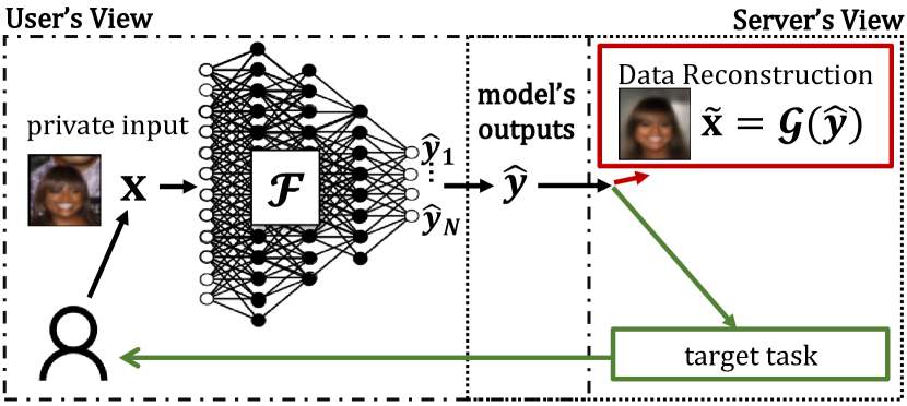
Figure 1. Processing user’s input ${\mathbf{x}}$, the server receives only the output $\hat{{\mathbf{y}}}\!=\!\mathcal{F}({\mathbf{x}})$. We show that for any model $\mathcal{F}$, the server can train an attack model $\mathcal{G}$ to secretly reconstruct the input from observed output, while providing the target service to the user with high accuracy.

To preserve privacy, current techniques are on-device (Teerapittayanon et al., 2017; Zhou et al., 2019) or encrypted (Gentry et al., 2013; Bourse et al., 2018) computations that hide inputs, as well as all the intermediate representations computed by the model, and only release the outputs to the server. Since such edge inferences for a target task might not seem sensitive to users’ privacy, the model’s outputs are released to the server in their raw form; as the server needs these outputs for performing their ultimate analyses and satisfying the services promised to the users. We argue that such a paradigm does not provide meaningful privacy protection for edge users.

As shown in Figure 1, we consider a common scenario of edge or encrypted inference, in which a user owns private data ${\mathbf{x}}$, and a semi-trusted server owns an $N$-output ML classifier $\mathcal{F}$. We put no constraint on the user’s access to $\mathcal{F}$; e.g., users can have a complete white-box view of $\mathcal{F}$. We assume that the server only observes the model’s output $\hat{{\mathbf{y}}}=\mathcal{F}({\mathbf{x}})$ (a.k.a. logits), which aims to help in predicting the target information ${\mathbf{y}}$. Our main assumption is that $\hat{{\mathbf{y}}}\in{\mathbb{R}}^{N}$ is a real-valued vector of dimension $N$, where each $\hat{{\mathbf{y}}}_{n}\in{\mathbb{R}}$, for all $n\in\{1,2,\dots,N\}$, is the logit score for the corresponding class or attribute ${\mathbf{y}}_{n}$. There are several reasons that a server might ask for observing the real-valued outputs $\hat{{\mathbf{y}}}$ to reach the ultimate decision at the server’s side; compared to only observing the $\operatorname*{argmax}({\hat{{\mathbf{y}}}})$ or softmax($\hat{{\mathbf{y}}}$). For example, the logit scores allow the server to perform top-K predictions, to measure the uncertainty in the estimation, to figure out adversarial or out-of-distribution samples, and more (Malinin and Gales, 2018).

The major contributions of our paper can be summarized as follows: (1) We show that high-capacity (i.e., overparameterized) deep neural networks (DNNs) can be trained viciously to efficiently encode additional information about their input data into the model’s outputs which are supposed to reveal nothing more than a specific target class or attribute: vicious classifiers. To this end, we propose jointly training a multi-task model $\mathcal{F}$ for building the required classifiers of target attributes as well as a decoder model $\mathcal{G}$, as the attack model, for reconstructing the input data from the shared outputs. We show that the trained $\mathcal{F}$ can not only be efficiently useful for the target task, but also secretly encode private information that can allow reconstructing the user’s personal data at inference time. Experimental results on MNIST, FMNIST, CIFAR10, CIFAR100, TinyImageNet, and CelebA datasets show that input data can be approximately reconstructed from just the outputs of a single inference.

(2) We discuss and compare the success of the malicious server in two settings: users share either the logits of $\mathcal{F}$ or the outputs after applying a softmax function. Experimental results show that, for the same model and with the softmax outputs, it is harder for an attacker to establish a good trade-off between the accuracy of target task and the quality of reconstructed data. Particularly, when the number of classes/attributes is less than $10$. However, for binary attributes, as sigmoid is a one-to-one function, the server can apply a simple trick: it can train the target model (as well as the corresponding attack model) on the logits, and after training it just attaches a sigmoid activation function to the output layer. It is clear that at inference time, the one-to-one property allows the server to easily transform the received sigmoid outputs into logits. While such a simple trick is unnoticeable to users and might make the released data less suspicious (than releasing the logits), it gives the server an attack performance as successful as releasing the logits.

(3) A missing aspect in existing data reconstruction attacks is a principal method for measuring the risk of reconstructed data. Previous works, e.g.,  (Zhu et al., 2019; Geiping et al., 2020; Yin et al., 2021), mostly borrow existing measures used in image/video compression literature; such as mean-squared error (MSE), peak signal-to-noise ratio (PSNR), or structural similarity index measure (SSIM). For instance, MSE (and thus PSNR) are based on the Euclidean distance that assumes features are not correlated to each other; which is rarely the case for real-world data types, such as images where pixels are highly correlated. The risk of a reconstruction attack depends not only on the similarity of the reconstruction to the original data, but also on the likelihood of that sample data. To this end, we propose a new measure of reconstruction success rate based on the Mahalanobis distance, which takes into account the covariance matrix of the data. Our proposed measure, called “reconstruction risk”, also offers a probabilistic view on data reconstruction attack and thus, offers a principled way to evaluate the success of an attack across models and datasets.

(4) A defense mechanism against data reconstruction attacks at inference time should be practical and ideally low-cost; considering the envisioned applications in edge computing. As emphasized in (Malekzadeh et al., 2021), distinguishing honest models from vicious ones is not trivial, and blindly applying perturbations to the outputs of all models can damage the utility received from honest servers. Users usually observe a trained model $\mathcal{F}$ that is claimed to be trained for a target task, but the exact training objective is unknown to them. Whether $\mathcal{F}$ only performs the claimed task or it also secretly performs another task is unknown. To this end, we propose a mechanism for estimating the likelihood of a model being vicious. Our proposed defense mechanism is based on the idea that a model trained only for the target task should not be far from the “ideal” solution for the target task; if it is only trained using the claimed objective function. On the other hand, if the model is vicious and is trained using another objective function to perform other tasks in parallel to the claimed one, then the model probably has not converged to the ideal solution for the target task. Our proposed defense is able to work even in black-box scenarios (e.g., encrypted computing), and provides a practical estimation for distinguishing honest vs. vicious models by only using a very small set of data points labeled for the target task.

Through uncovering a major risk in using powerful ML services, our work has implications for advancing privacy protection for the users’ of such ML services. We believe our proposed analysis is just a first look, thus we conclude this paper by discussing current challenges and open directions for future investigations. We publish our code for reproducing the reported results here.

2. Related Work

There are several attacks on data privacy in ML, such as property inference (Melis et al., 2019), membership inference (Shokri et al., 2017; Salem et al., 2018; Carlini et al., 2019), model inversion for data reconstruction (Fredrikson et al., 2015; Zhu et al., 2019), or model poisoning (Biggio et al., 2012; Muñoz-González et al., 2017; Jagielski et al., 2018). However, these attacks target training data, or they happen after multiple rounds of interactions, during which large amounts of information are shared with untrusted parties. Regarding attacks at inference time on test data, (Song and Shmatikov, 2020) showed that due to “overlearning”, the internal representations extracted by DNN layers can reveal private attributes of the input data that might not even be correlated to the target attribute. But, in (Song and Shmatikov, 2020) the adversary is allowed to observe a subset of internal representations. Our work considers data privacy at inference time, where the private input as well as all the internal representations are hidden, and the adversary has access only to the model’s outputs.

A recent work (Malekzadeh et al., 2021) shows that when users only release the model’s output, “overlearning” is not a major concern as standard models do not reveal significant information about another private attribute. But ML models can be trained to be “honest-but-curious” (Malekzadeh et al., 2021) and to secretly reveal a private attribute just through the model’s output for a target attribute. While they show how to encode a single private attribute into the output of a model intended for another target attribute, in our work we show how by having access only to the model’s outputs we can reconstruct the entire input data, and consequently infer many private attributes. An untrusted server in (Malekzadeh et al., 2021) needs to decide the private attribute that they want to infer at training time, but in this paper, we do not need to choose a specific private attribute at training time, as we reconstruct the whole input data.

In (Luo et al., 2021; Jiang et al., 2022), vertical federated learning is considered, where there are two parties, each observing a subset of the features for the same set of samples. An untrusted party can reconstruct the values of the private scalar features owned by the other party only from the output of a model that both parties jointly train. A generative model is used to estimate the values of the private features assuming that the malicious party can make multiple queries on the same data of the victim party. However, the problem setting and threat model of (Luo et al., 2021; Jiang et al., 2022) are quite different from our work as instead of two collaborating agents, we consider servers and their users, where each user owns a single data point, and shares the output of the model only once. Moreover, in (Luo et al., 2021; Jiang et al., 2022), it is assumed that the trained model is under the adversary’s control at inference time, but in our work, we assume that training is already performed by the server on another dataset, and the model is under the user’s control at inference time.

Overall, our work is the first showing that ML service providers can perform the strongest attack to data privacy (i.e., data reconstruction attack) at inference time, and such an attack is possible even in a highly restricted scenario, in which the server observes only the outputs that are aimed for the target task, and even when data is not just a scalar but it is multi-dimensional; such as face images.

3. Methodology

We formulate the problem and introduce the required definitions (§3.1). We then present the training algorithm for jointly training the public classifiers and the attack model for data reconstruction (§3.2). We provide an analysis of the relation between the entropy of the model’s output and the privacy risk of data reconstruction (§3.3). Finally, we define our proposed measure of reconstruction risk (§3.4).

3.1. Problem Formulation

Let $\mathcal{X}\times\mathcal{Y}$ denote the joint distribution over data and labels (or attributes). We assume that each data point $({\mathbf{x}},{\mathbf{y}})\sim(\mathcal{X}\times\mathcal{Y})$ either (1) exclusively belongs to one of the $N$ classes (i.e., categorical $\mathcal{Y}=\{1,2,\dots,N\}$), or (2) has $N$ binary attributes (i.e., $\mathcal{Y}=\{0,1\}^{N}$). Let the server train a model $\mathcal{F}$ on a target task $\mathcal{Y}$, where $\mathcal{F}({\mathbf{x}})=\hat{{\mathbf{y}}}=[\hat{{\mathbf{y}}}_{1},\hat{{\mathbf{y}}}_{2},\dots,\hat{{\mathbf{y}}}_{N}]$ denotes the model’s outputs; i.e., prediction scores (logits) over $\mathcal{Y}$. For the categorical case, $\mathcal{Y}=\{1,2,\dots,N\}$, each $\hat{{\mathbf{y}}}_{i}$ shows the logit score for the class $i$ (e.g., the score for class $i$ in CIFAR10 dataset). For the binary case, $\mathcal{Y}=\{0,1\}^{N}$, each $\hat{{\mathbf{y}}}_{i}$ shows the logit score for the attribute $i$ (e.g., the score for attribute $i$ in CelebA dataset, such as “smiling” attribute).

We allow $\mathcal{F}$ to have any arbitrary architecture; e.g., to be a single model with $N$ outputs, or to be an ensemble of $N$ models each with a single output, or any other architectural choice. At inference time, the users will have a complete white-box view of $\mathcal{F}$. We consider two settings: (1) logit outputs, where $\hat{{\mathbf{y}}}\in{\mathbb{R}}^{N}$, and (2) softmax outputs, where using the standard softmax function, $\hat{{\mathbf{y}}}$ is normalized to a probability distribution over the possible classes.

3.1.1. Model’s Utility

Let ${\mathbb{1}}(\mathrm{C})$ denote the indicator function that outputs 1 if condition $\mathrm{C}$ holds, and 0 otherwise. Given a test dataset ${\mathbb{D}}^{test}\sim(\mathcal{X},\mathcal{Y})$, we define the model’s accuracy in performing the target task $\mathcal{Y}$ as either:

(1) $$Acc\equiv\Pr_{({\mathbf{x}},{\mathbf{y}})\sim{\mathbb{D}}^{test},\text{ }\hat{{\mathbf{y}}}\leftarrow\mathcal{F}({\mathbf{x}})}\big{[}{\mathbb{1}}\big{(}\operatorname*{argmax}(\hat{{\mathbf{y}}})={\mathbf{y}}\big{)}\big{]},$$

when ${\mathbf{y}}$ denotes a categorical attribute, or

(2) $$Acc\equiv\frac{1}{N}\sum_{n=1}^{N}\Pr_{({\mathbf{x}},{\mathbf{y}}_{n})\sim{\mathbb{D}}^{test},\text{ }\hat{{\mathbf{y}}}_{n}\leftarrow\mathcal{F}({\mathbf{x}})}[{\mathbb{1}}(\hat{{\mathbf{y}}}_{n}>\tau_{n})={\mathbf{y}}_{n}],$$

when ${\mathbf{y}}_{n}$ denotes the $n$-th binary attribute and $\tau_{n}$ is the chosen threshold for that attribute. Usually, $\tau_{n}=0$ for the logit outputs and $\tau_{n}=0.5$ for softmax outputs (which is equivalent to sigmoid outputs for binary attributes).

3.1.2. Data Privacy

Our assumption is that a user shares the computed outputs with the server, and this is the only information that the server can get access to. The server is supposed to perform only the target task and not infer any information other than the pre-specified target class/attributes. In particular, the server should not be able to (approximately) reconstruct the user’s private data ${\mathbf{x}}$.

We show the possibility that the server can build an attack function $\mathcal{G}$ for the reconstruction of the user’s private data from the received outputs; i.e., $\widetilde{\mathbf{x}}=\mathcal{G}(\hat{{\mathbf{y}}})$. We define $\mathcal{S}(\cdot,\cdot)$ as a measure of reconstruction risk, and $\mathcal{S}(\widetilde{\mathbf{x}},{\mathbf{x}})\geq\mathtt{R}$ means that the risk of reconstructing ${\mathbf{x}}$ is more than $\mathtt{R}$ based on the measure $\mathcal{S}$. Examples of such $\mathcal{S}$ in the literature are PSNR for general signals and SSIM for images. Thus, before measuring the privacy risk of a model, regarding data reconstruction attack, we first need to define $\mathcal{S}$; as we do in our evaluations.

We say a classifier is vicious if it is trained with an objective function that captures private information (beyond the target task) in the model’s output. We refer to models that are only trained for the target task as honest models.

3.1.3. Curious vs. Vicious

As mentioned in §2,  (Malekzadeh et al., 2021) shows that ML models can be trained to be “honest-but-curious” and to reveal a private attribute just through the model’s output for a target attribute. In our work, we coin the term vicious classifier to distinguish it from a curious classifier in (Malekzadeh et al., 2021). A curious classifier is trained to encode a single private attribute into the output of a model intended for another target attribute, and a vicious classifier aims to reconstruct the entire input data, and consequently might infer many private attributes. Moreover, for a curious classifier in (Malekzadeh et al., 2021), the untrusted server selects the private attributes that they want to infer a priori at training time, but for a vicious classifier there is no need to choose a specific private attribute at training time, as we reconstruct the whole input data.

3.2. Training of Target and Attack Models

We present an algorithm for jointly training $\mathcal{F}$ and $\mathcal{G}$. As shown in Figure 2, the server trains a model $\mathcal{F}$ that takes data ${\mathbf{x}}$ as input and produces $N$-outputs. Outputs are attached to the classification loss function $L^{C}$, which computes the amount of inaccuracy in predicting the true attribute ${\mathbf{y}}$, and thus provides gradients for updating $\mathcal{F}$. For categorical attributes, we use the standard categorical cross-entropy loss

(3) $$L^{C}(\hat{{\mathbf{y}}},{\mathbf{y}})=\sum_{n=1}^{N}-{\mathbf{y}}_{n}\log\hat{{\mathbf{y}}}_{n}\text{,}$$

and for binary attributes, we use the class-weighted binary cross-entropy

(4) $$L^{C}(\hat{{\mathbf{y}}},{\mathbf{y}})=\frac{1}{N}\sum_{n=1}^{N}\eta_{n}{\mathbf{y}}_{n}\log\hat{{\mathbf{y}}}_{n}+(1-{\mathbf{y}}_{n})\log(1-\hat{{\mathbf{y}}}_{n}),$$

where $\eta_{n}$ denotes the weight of class 1 for attribute ${\mathbf{y}}_{n}\in\{0,1\}$, and it is defined as the number of samples labeled $0$ divided by the number of samples labeled $1$ in the training dataset. CelebA dataset (Liu et al., 2015) used in our experiments is highly unbalanced for several attributes. Our motivation for using the class-weighted binary loss function is to obtain a fairer classification for unbalanced labels.

While training $\mathcal{F}$, the model’s outputs are fed into another model $\mathcal{G}$, which aims to reconstruct the original data. The output of $\mathcal{G}$ is attached to a reconstruction loss function $L^{R}$, producing gradients for updating both $\mathcal{F}$ and $\mathcal{G}$.

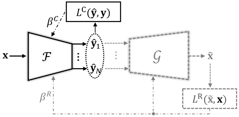
Figure 2. Joint training; $\mathcal{F}$ is the target model, $\mathcal{G}$ is the attack model, $L^{C}$ is the classification loss, $L^{R}$ is the reconstruction loss of the attack. Both $\mathcal{F}$ and $\mathcal{G}$ are DNNs. Hyperparameters $\beta^{C}$ and $\beta^{R}$ control the trade-offs between classification and reconstruction tasks.

In this paper, we benchmark image datasets in our experiments; thus, we utilize the loss functions used in image processing tasks (Zhao et al., 2016). In particular, we employ a weighted sum of $(i)$ structural similarity index measure (SSIM) (Wang et al., 2004) and $(ii)$ Huber loss (Hastie et al., 2009) which is a piecewise function including both mean squared error (known as MSELoss) and mean absolute error (MAE, also known as L1Loss) (Paszke et al., 2019). This design choice of combining a perceptually-motivated loss (i.e., SSIM) with a statistically-motivated loss (i.e., MSELoss or L1Loss) is inspired by the common practice used by previous work in image-processing literature (Zhao et al., 2016; Yoo and Chen, 2021).

$(i)$ SSIM is built on the idea that an image’s pixels have strong inter-dependencies especially when they are spatially close. The SSIM index between image ${\mathbf{x}}$ and its reconstruction $\widetilde{\mathbf{x}}$ is defined as:

(5) $$SSIM(\widetilde{\mathbf{x}},{\mathbf{x}})=\frac{\big{(}2\mu_{{\mathbf{x}}}\mu_{\widetilde{\mathbf{x}}}+(k_{1}L)^{2}\big{)}\big{(}2\sigma_{{\mathbf{x}}\widetilde{\mathbf{x}}}+(k_{2}L)^{2}\big{)}}{\big{(}\mu^{2}_{{\mathbf{x}}}+\mu^{2}_{\widetilde{\mathbf{x}}}+(k_{1}L)^{2}\big{)}\big{(}\sigma_{{\mathbf{x}}}+\sigma_{\widetilde{\mathbf{x}}}+(k_{2}L)^{2}\big{)}},$$

where $\mu_{{\mathbf{x}}}$ (similarly $\mu_{\widetilde{\mathbf{x}}}$), $\sigma_{{\mathbf{x}}}$ (similarly $\sigma_{\widetilde{\mathbf{x}}}$), and $\sigma_{{\mathbf{x}}\widetilde{\mathbf{x}}}$ denote the average, variance, and co-variance values, respectively. Here, $L$ denotes the size of the range of pixel values. We normalize the pixel values to the range $[0,1]$, and hence, $L=1$. We use the default values of $k_{1}=0.01$, $k_{2}=0.03$, and the default window size $11\times 11$. The SSIM in Equation (5) is computed for every window, and the mean SSIM value among all the windows is considered as the final similarity index between two images. As SSIM lies within $[0,1]$, $SSIM(\widetilde{\mathbf{x}},{\mathbf{x}})=1$ is seen as the perfect reconstruction.

$(ii)$ Huber loss computes the mean squared error (MSE) if the absolute pixel-wise error falls below its parameter $\delta$; otherwise, it uses $\delta$-scaled mean absolute error (the default value for $\delta=1$). Thus, Huber loss combines advantages of both MSE and L1 losses; as the L1 term is less sensitive to outliers, and the MSE term provides smoothness near 0:

(6) $$Huber(\widetilde{\mathbf{x}},{\mathbf{x}})=\begin{cases}0.5\text{MSELoss}(\widetilde{\mathbf{x}},{\mathbf{x}})&\text{if }\text{L1Loss}({\widetilde{\mathbf{x}},{\mathbf{x}}})<\delta\\ \delta(\text{L1Loss}({\widetilde{\mathbf{x}},{\mathbf{x}}})-0.5\delta)&otherwise.\end{cases}$$

The minimum value of Huber loss is 0 (i.e., perfect reconstruction), and the maximum value depends on the input data dimensions. Thus, we need some hyperparameters to regularize the importance of structural similarity loss (SSIM) compared to the pixel-wise reconstruction loss (Huber). The combined reconstruction loss is:

(7) $$L^{R}(\widetilde{\mathbf{x}},{\mathbf{x}})=\alpha SSIM(\widetilde{\mathbf{x}},{\mathbf{x}})+\gamma Huber(\widetilde{\mathbf{x}},{\mathbf{x}}),$$

where $\alpha$ and $\gamma$ are the hyperparameters for data reconstruction. Note that, depending on the data type and the attack’s purpose, one can use other reconstruction loss functions.

The ultimate loss function. We use the following loss function for optimizing the parameters of $\mathcal{F}$:

(8) $$L^{\mathcal{F}}=\beta^{C}L^{C}(\hat{{\mathbf{y}}},{\mathbf{y}})+\beta^{R}L^{R}(\widetilde{\mathbf{x}},{\mathbf{x}}),$$

where $\beta^{C}$ and $\beta^{R}$ are the weights that allow us to move along different possible local minimas and both are non-negative real-valued. For optimizing the parameters of $\mathcal{G}$, we only use $L^{R}$, but notice that there is an implicit connection between $\mathcal{G}$, $\mathcal{F}$, and $L^{C}$ since $\mathcal{G}$ acts on $\hat{{\mathbf{y}}}=\mathcal{F}({\mathbf{x}})$. Algorithm 1 summarizes the explained training procedure.

Algorithm 1 Training classifier $\mathcal{F}$ and attack model $\mathcal{G}$.

1:  Input: $\mathcal{F}$: an $N-$output classifier, $\mathcal{G}$: $N-$input data reconstruction model, ${\mathbb{D}}^{train}$: training set, ${\mathbb{D}}^{valid}$: validation set, $(\beta^{C},\beta^{R})$: classification-reconstruction trade-off multipliers, $E$: number of epochs, $K$: batch size, $L^{C}$: classification loss, $L^{R}$: reconstruction loss, $OPT^{\mathcal{F}}$ and $OPT^{\mathcal{G}}$: optimizers for $\mathcal{F}$ and $\mathcal{G}$.

2:  Output: trained classifier $\mathcal{F}$ and attack model $\mathcal{G}$,

3:  begin

4:  $\mathcal{F},\mathcal{G}=randomly\_initialize(\mathcal{F}),randomly\_initialize(\mathcal{G})$

5:  best_validation_result = 0

6:  for $e:1,\ldots,E$ do

7:     for $b:1,\ldots,|{\mathbb{D}}^{train}|/K$ do

8:        $Loss^{C}=\text{ }Loss^{R}=0$

9:        for $k:1,\ldots,K$ do

10:           $({\mathbf{x}},{\mathbf{y}})\sim{\mathbb{D}}^{train}$ $\#$ random uniform sampling

11:           $\hat{{\mathbf{y}}}=\mathcal{F}({\mathbf{x}})$

12:           $Loss^{C}=Loss^{C}+L^{C}(\hat{{\mathbf{y}}},{\mathbf{y}})$ $\#$ Equation (3) or (4)

13:           $\widetilde{\mathbf{x}}=\mathcal{G}(\hat{{\mathbf{y}}})$

14:           $Loss^{R}=Loss^{R}+L^{R}(\widetilde{\mathbf{x}},{\mathbf{x}})$ $\#$ Equation (7)

15:        end for

16:        $Loss^{C}=Loss^{C}/(K)$

17:        $Loss^{R}=Loss^{R}/(K)$

18:        $\mathcal{F}=OPT^{\mathcal{F}}(\beta^{C}Loss^{C}+\beta^{R}Loss^{R})$ $\#$ Equation (8)

19:        $\mathcal{G}=OPT^{\mathcal{G}}(\beta^{R}Loss^{R})$

20:     end for

21:     result = $evaluate(\mathcal{F},\mathcal{G},\beta^{C},\beta^{R},{\mathbb{D}}^{valid})$ $\#$

22:     if result $\geq$ best_validation_result then

23:        best_validation_result = result

24:        $\mathcal{F}^{\prime},\text{ }\mathcal{G}^{\prime}=\mathcal{F},\text{ }\mathcal{G}$

25:     end if

26:  end for

27:  return  $\mathcal{F}^{\prime}\text{ and }\mathcal{G}^{\prime}$

3.3. An Information-Theoretical View

The objective function in Equation (8) can also be formulated as the optimization function

(9) $$\max\ {\mathtt{I}}({\mathbf{x}},\hat{{\mathbf{y}}})\ \ \text{ {subject to}}\ \operatorname*{argmax}(\hat{{\mathbf{y}}})={\mathbf{y}}.$$

The “penalty method” (Boyd and Vandenberghe, 2004) can be used to replace a constrained optimization problem with an unconstrained problem, whose solution ideally converges to the solution of the original constrained problem. The unconstrained formulation is

(10) $$\max\ {\mathtt{I}}({\mathbf{x}},\hat{{\mathbf{y}}})+\beta\ {\mathbb{1}}(\operatorname*{argmax}(\hat{{\mathbf{y}}})={\mathbf{y}}),$$

where hyperparameter $\beta$ is called the “penalty parameter”.

This formulation can be particularly appropriate when the server does not know what type of reconstruction measure (SSIM, MSE, L1, etc.) will be more relevant for the attack. Hence, instead of training for a specific reconstruction measure, the server can try to capture as much information about ${\mathbf{x}}$ as it can into the model’s output $\hat{{\mathbf{y}}}$ (the first term in Equation (10)), and the server’s only constraint is to keep the output informative for the target classification task (the second term in Equation (10)). The indicator function in Equation (10) is not easy to use by existing optimization tools, but one can re-write the formula via a surrogate function as

(11) $$\max\ {\mathtt{I}}({\mathbf{x}},\hat{{\mathbf{y}}})-\beta H_{{\mathbf{y}}}(\hat{{\mathbf{y}}}),$$

where instead of maximizing the indicator function we minimize the cross-entropy function $H_{{\mathbf{y}}}(\hat{{\mathbf{y}}})=-\sum_{n=1}^{N}{\mathbf{y}}_{n}\log\hat{{\mathbf{y}}}_{n}$, as in Equation (3). This problem then is equivalent to

(12) $$\max\ {\mathtt{H}}(\hat{{\mathbf{y}}})-{\mathtt{H}}(\hat{{\mathbf{y}}}|{\mathbf{x}})-\beta H_{{\mathbf{y}}}(\hat{{\mathbf{y}}}).$$

As most of the classifiers in practice are deterministic functions, we have ${\mathtt{H}}(\hat{{\mathbf{y}}}|{\mathbf{x}})=0$, and the optimization problem becomes

(13) $$\max\ {\mathtt{H}}(\hat{{\mathbf{y}}})-\beta\ {\mathtt{H}}_{{\mathbf{y}}}(\hat{{\mathbf{y}}}).$$

We know that ${\mathtt{H}}_{{\mathbf{y}}}(\hat{{\mathbf{y}}})\geq{\mathtt{H}}({\mathbf{y}}|\hat{{\mathbf{y}}})$, as one can prove it in the following way:

(14) $$\begin{split}&{\mathtt{H}}_{{\mathbf{y}}}(\hat{{\mathbf{y}}})={\mathtt{H}}({\mathbf{y}})-{\mathtt{H}}({\mathbf{y}})+{\mathtt{H}}_{{\mathbf{y}}}(\hat{{\mathbf{y}}})\\ &=-\sum_{n=1}^{N}{\mathbf{y}}_{n}\log{\mathbf{y}}_{n}+\sum_{n=1}^{N}{\mathbf{y}}_{n}\log{\mathbf{y}}_{n}-\sum_{n=1}^{N}{\mathbf{y}}_{n}\log\hat{{\mathbf{y}}}_{n}\\ &=-\sum_{n=1}^{N}{\mathbf{y}}_{n}\log{\mathbf{y}}_{n}+\sum_{n=1}^{N}{\mathbf{y}}_{n}\log(\frac{{\mathbf{y}}_{n}}{\hat{{\mathbf{y}}}_{n}})\\ &={\mathtt{H}}({\mathbf{y}})+D_{KL}({\mathbf{y}}||\hat{{\mathbf{y}}})={\mathtt{H}}({\mathbf{y}}|\hat{{\mathbf{y}}})+{\mathtt{I}}({\mathbf{y}};\hat{{\mathbf{y}}})+D_{KL}({\mathbf{y}}||\hat{{\mathbf{y}}})\geq{\mathtt{H}}({\mathbf{y}}|\hat{{\mathbf{y}}}),\end{split}$$

where the last inequality is based on the fact that both mutual information and Kullback–Leibler divergence are non-negative. Therefore, any solution for the optimization problem of (13) provides a lower bound on the below formula

(15) $$\max\ {\mathtt{H}}(\hat{{\mathbf{y}}})-\beta\ {\mathtt{H}}({\mathbf{y}}|\hat{{\mathbf{y}}}).$$

This sheds light on the attack’s objective: the attacker aims to maximize the entropy of the output while keeping the outputs informative about the target information. Therefore, as long as the attacker keeps the outputs informative about the target task, they can use the rest of the information capacity (i.e., the output’s entropy) to capture other private information. Thus, a vicious model should produce higher-entropy outputs than an honest model. Inspired by this fact, we introduce a defense mechanism to distinguish vicious models in §5.

3.4. Reconstruction Risk

As noted in §3.1, we define $\mathcal{S}(\cdot,\cdot)$ as a measure of reconstruction risk, and $\mathcal{S}(\widetilde{\mathbf{x}},{\mathbf{x}})\geq\mathtt{R}$ means that the risk of reconstructing ${\mathbf{x}}$ is more than $\mathtt{R}$ based on the measure $\mathcal{S}$. Considering the reconstruction of data, $\widetilde{\mathbf{x}}$, we use $\mathcal{S}$ to evaluate the attack’s success or the amount of privacy loss. Here, a pivotal question is what is the most suitable and general $\mathcal{S}$ for computing and evaluating the attacker’s success. Previous works, mentioned in §2, ignored answering this question, and they mostly rely on common measures such as MSE or SSIM. In this section, we propose a new measure of reconstruction risk and, in §4, we compare our proposed measure with other measures borrowed from other applications.

Basics. Having two random vectors ${\mathbf{x}}$ and $\widetilde{\mathbf{x}}$ of the same distribution with covariance matrix $\mathbf{\Sigma_{\mathbb{D}}}$, the Mahalanobis distance (MD) is a dissimilarity measure between ${\mathbf{x}}$ and $\widetilde{\mathbf{x}}$:

(16) $$\mathsf{d}({\mathbf{x}},\widetilde{\mathbf{x}})=\sqrt{({\mathbf{x}}-\widetilde{\mathbf{x}})\mathbf{\Sigma_{\mathbb{D}}}^{-1}({\mathbf{x}}-\widetilde{\mathbf{x}})}.$$

Similarly, we can compute $\mathsf{d}({\mathbf{x}},\mu_{\mathbb{D}})$, where $\mu_{\mathbb{D}}$ is the mean of the distribution that ${\mathbf{x}}$ is drawn from. One can notice that if $\mathbf{\Sigma_{\mathbb{D}}}$ is the identity matrix, the MD reduces to the Euclidean distance (and thus the typical MSE). Notice that in practice, e.g., for real-world data types such as images, the $\mathbf{\Sigma_{\mathbb{D}}}$ is rarely close to the identity matrix. The pixels of an image are correlated to each other. Similarly, the sample points of time-series signals are temporally correlated to each other, and so on. Therefore, for computing MD, we need to approximate $\mathbf{\Sigma_{\mathbb{D}}}$ using a sample dataset. In our experiments, we approximate $\mathbf{\Sigma_{\mathbb{D}}}$ via samples in the training dataset.

Another characteristic of MD is that when the data comes from a multivariate normal distribution, the probability density of an observation ${\mathbf{x}}$ is uniquely determined by MD:

(17) $$\Pr({\mathbf{x}})=\frac{1}{\sqrt{det(2\pi\mathbf{\Sigma_{\mathbb{D}}})}}\exp\Big{(}-\frac{(\mathsf{d}({\mathbf{x}},\mu_{\mathbb{D}})\big{)}^{2}}{2}\Big{)}.$$

The multivariate normal distribution is the most common probability distribution that is used for approximating data distribution (Murphy, 2021). And thus, with the assumption that one can approximate data distribution using a multivariate normal distribution, MD can be utilized for computing the probability density of an observation ${\mathbf{x}}$; i.e., $\Pr({\mathbf{x}})$.

Our Measure. Motivated by the characteristics of MD, we argue that the risk of a reconstruction $\widetilde{\mathbf{x}}$ of a sample ${\mathbf{x}}$ depends on both $\mathsf{d}({\mathbf{x}},\widetilde{\mathbf{x}})$ and $\Pr({\mathbf{x}})$: the more unlikely is a sample (lower $\Pr({\mathbf{x}})$), the more important is the value of $\mathsf{d}({\mathbf{x}},\widetilde{\mathbf{x}})$ (the more informative is a specific reconstruction). In other words, for the reconstructions of two independent samples ${\mathbf{x}}^{1}$ and ${\mathbf{x}}^{2}$ with $\mathsf{d}({\mathbf{x}}^{1},\widetilde{\mathbf{x}}^{1})=\mathsf{d}({\mathbf{x}}^{2},\widetilde{\mathbf{x}}^{2})$ and $\Pr({\mathbf{x}}^{1})<\Pr({\mathbf{x}}^{2})$, the risk of $\widetilde{\mathbf{x}}^{1}$ should be higher than $\widetilde{\mathbf{x}}^{2}$. The intuition is: because ${\mathbf{x}}^{1}$ is less likely than ${\mathbf{x}}^{2}$, then ${\mathbf{x}}^{1}$ is easier to be identified when the attacker observes $\widetilde{\mathbf{x}}^{1}$, compared to ${\mathbf{x}}^{2}$ when the attacker observes $\widetilde{\mathbf{x}}^{2}$. In other words, because ${\mathbf{x}}^{1}$ is less likely (or more unique) than ${\mathbf{x}}^{2}$, then a reconstruction of ${\mathbf{x}}^{1}$ will give the attacker more information.

In general, the intuition is that reconstructing a data point that belongs to a more sparse part of the population is riskier than reconstructing those that belong to a more dense part of the population. To this end, we define the reconstruction risk of a model with respect to a benchmark test dataset $\mathbb{D}=\{x^{n}\}_{n=1}^{N}$ as

(18) $$\mathtt{R}=\frac{1}{N}\sum_{n=1}^{N}\mathsf{d}({\mathbf{x}}^{n},\mu_{\mathbb{D}})\big{/}\mathsf{d}({\mathbf{x}}^{n},\widetilde{\mathbf{x}}^{n}).$$

The less likely a sample, or the better its reconstruction quality, the higher is its contribution to the risk of the benchmark dataset. Our measure gives a general notion of reconstruction risk that depends on the characteristics of the entire dataset, and not just each sample independently (as PSNR and SSIM do). Moreover, our measure can be used across different data types and is not restricted to images or videos.

Remark. Our proposed $\mathtt{R}$ is task-agnostic, which has some advantages. However, it also has limitations in situations where the reconstruction is judged by a specific task. For example, for face images, the reconstruction of the background might not be as important as the reconstruction of the eyes or mouth. One needs to perform some preprocessing for task-specific risk assessments, for example, by running a segmentation algorithm and applying the computation of $\mathtt{R}$ only to that segment of the photo that shows the face. We leave exploration of this aspect to future studies.

4. Experimental Results

We explain our experimental setup (§4.1), present results on several datasets and settings, and compare reconstruction risk $\mathtt{R}$ with other common measures, PSNR and SSIM (§4.2).

4.1. Setup

4.1.1. Datasets

Table 1 lists the datasets we use for evaluations. We use benchmark datasets of different complexity to measure the performance of the attackers in different scenarios. MNIST, FMNIST, and CIFAR10 all have 10 classes, but the complexity of their data types are quite different. CIFAR10, CIFAR100, and TinyImgNet are of (almost) the same data type complexity, but their number of classes is different. CelebA is a dataset including more than 200K celebrity face images, each with 40 binary attributes, e.g., the ‘Smiling’ attribute with values $0$:$Non\text{-}Smile$ or $1$:$Smile$. Just a few of these attributes are balanced (having almost equal numbers of 0s and 1s). For the results reported in Table 3, when we want to choose $K$ attributes, we choose the $K$ most balanced ones. For a fair comparison among datasets, we reshape all the images to the same width and height of $32$. All datasets are split into training and test sets, by the publishers. For the validation set during training, we randomly choose 10% of training data and perform the training only on the rest 90%; except for CelebA, which the publisher has already included a validation set.

Table 1. Datasets used in our experiments.

Labels	Dataset (ref.)	Classes	Shape	Samples
Categorical	MNIST (LeCun, 1998)	10	32$\times$32$\times$1	60K
	FMNIST (Xiao et al., 2017)	10	32$\times$32$\times$1	60K
	CIFAR10 (Krizhevsky et al., 2009)	10	32$\times$32$\times$3	50K
	CIFAR100 (Krizhevsky et al., 2009)	100	32$\times$32$\times$3	50K
	TinyImgNet (Le and Yang, 2015)	200	32$\times$32$\times$3	100K
Binary	CelebA (Liu et al., 2015)	40	32$\times$32$\times$3	200K

4.1.2. Models and Training

For $\mathcal{F}$ and $\mathcal{G}$ in Figure 1, we borrow one of the commonly-used architectures for data classification: WideResNet (Zagoruyko and Komodakis, 2016). WideResNet allows decreasing the depth of the model (i.e., the number of layers) and instead increases the width of the residual networks; which has shown better performance over other thin and very deep counterparts. For $\mathcal{F}$, we use WideResNet of width 5 which has around 9M parameters. For $\mathcal{G}$, we use an architecture similar to that of $\mathcal{F}$, but we replace the convolutional layers with transpose-convolutional layers. For all the experiments, we use a batch size of 250 images, and Adam optimizer (Kingma and Ba, 2014) with a learning rate of $0.001$.

4.1.3. Settings

Each experiment includes training $\mathcal{F}$ and $\mathcal{G}$ on the training dataset based on Algorithm 1, for 50 epochs, and choosing $\mathcal{F}$ and $\mathcal{G}$ of the epoch in which we achieve the best result on the validation set according to loss function in Equation (8). In each experiment, via the test dataset, we evaluate $\mathcal{F}$ by measuring the accuracy of $\mathcal{F}$ in estimating the public task using Equations (1) or (2), and we evaluate $\mathcal{G}$ by computing the reconstruction quality measured by PSNR, SSIM, and our proposed reconstruction risk $\mathtt{R}$ in  (18). To compute $\mathtt{R}$, we approximate $\mu_{\mathbb{D}}$ and $\mathbf{\Sigma_{\mathbb{D}}}$ via samples in the training set. For a fair comparison, we use a random seed that is fixed throughout all the experiments, thus the same model initialization and data sampling are used.

4.2. Results

Table 2. Reconstruction quality vs. classification accuracy in different settings and for different datasets. We repeat each experiment for five different random seed and report the mean and standard deviation.

Outputs	Dataset	$\beta^{R}/\beta^{C}$	PSNR (dB)	SSIM	$\mathtt{R}$	ACC (%)
Logits	MNIST	$0/1$	0.000 $\pm$ 0.000	0.000 $\pm$ 0.000	1.000 $\pm$ 0.000	99.54 $\pm$ 0.11
		$1/1$	22.090 $\pm$ 0.095	0.920 $\pm$ 0.003	1.378 $\pm$ 0.021	99.53 $\pm$ 0.09
		$3/1$	22.367 $\pm$ 0.075	0.926 $\pm$ 0.001	1.394 $\pm$ 0.012	99.52 $\pm$ 0.04
		$5/1$	22.336 $\pm$ 0.049	0.927 $\pm$ 0.001	1.392 $\pm$ 0.011	99.55 $\pm$ 0.04
		$1/0$	22.169 $\pm$ 0.052	0.926 $\pm$ 0.001	1.398 $\pm$ 0.009	10.00 $\pm$ 0.00
	FMNIST	$0/1$	0.000 $\pm$ 0.000	0.000 $\pm$ 0.000	1.000 $\pm$ 0.000	94.33 $\pm$ 0.12
		$1/1$	20.525 $\pm$ 0.056	0.783 $\pm$ 0.001	1.243 $\pm$ 0.003	94.58 $\pm$ 0.05
		$3/1$	20.883 $\pm$ 0.061	0.799 $\pm$ 0.001	1.272 $\pm$ 0.006	94.24 $\pm$ 0.08
		$5/1$	20.871 $\pm$ 0.068	0.803 $\pm$ 0.001	1.271 $\pm$ 0.004	94.30 $\pm$ 0.16
		$1/0$	21.021 $\pm$ 0.032	0.810 $\pm$ 0.001	1.281 $\pm$ 0.008	10.00 $\pm$ 0.00
	CIFAR10	$0/1$	0.000 $\pm$ 0.000	0.000 $\pm$ 0.000	1.000 $\pm$ 0.000	91.86 $\pm$ 0.69
		$1/1$	15.388 $\pm$ 0.039	0.377 $\pm$ 0.002	1.009 $\pm$ 0.003	91.34 $\pm$ 0.58
		$3/1$	15.550 $\pm$ 0.042	0.406 $\pm$ 0.001	1.013 $\pm$ 0.001	90.84 $\pm$ 0.35
		$5/1$	15.581 $\pm$ 0.043	0.414 $\pm$ 0.003	1.010 $\pm$ 0.003	90.62 $\pm$ 0.62
		$1/0$	15.784 $\pm$ 0.037	0.468 $\pm$ 0.000	1.026 $\pm$ 0.002	10.00 $\pm$ 0.00
	CIFAR100	$0/1$	0.000 $\pm$ 0.000	0.000 $\pm$ 0.000	1.000 $\pm$ 0.000	68.13 $\pm$ 0.66
		$1/1$	16.757 $\pm$ 0.142	0.473 $\pm$ 0.012	1.051 $\pm$ 0.003	67.50 $\pm$ 0.66
		$3/1$	18.463 $\pm$ 0.311	0.646 $\pm$ 0.018	1.147 $\pm$ 0.023	64.57 $\pm$ 1.20
		$5/1$	19.047 $\pm$ 0.235	0.701 $\pm$ 0.008	1.201 $\pm$ 0.015	61.25 $\pm$ 1.34
		$1/0$	20.693 $\pm$ 0.097	0.821 $\pm$ 0.002	1.454 $\pm$ 0.011	1.00 $\pm$ 0.00
	TinyImgNet	$0/1$	0.000 $\pm$ 0.000	0.000 $\pm$ 0.000	1.000 $\pm$ 0.000	46.96 $\pm$ 0.25
		$1/1$	16.763 $\pm$ 0.171	0.473 $\pm$ 0.014	1.042 $\pm$ 0.004	45.98 $\pm$ 0.56
		$3/1$	19.036 $\pm$ 0.190	0.692 $\pm$ 0.011	1.166 $\pm$ 0.016	42.71 $\pm$ 0.22
		$5/1$	20.072 $\pm$ 0.181	0.766 $\pm$ 0.009	1.261 $\pm$ 0.019	37.57 $\pm$ 1.39
		$1/0$	23.166 $\pm$ 0.104	0.900 $\pm$ 0.004	1.796 $\pm$ 0.028	0.50 $\pm$ 0.00
	CelebA	$0/1$	0.000 $\pm$ 0.000	0.000 $\pm$ 0.000	1.000 $\pm$ 0.000	88.43 $\pm$ 0.00
		$1/1$	19.081 $\pm$ 0.044	0.813 $\pm$ 0.000	1.238 $\pm$ 0.002	88.03 $\pm$ 0.06
		$3/1$	19.619 $\pm$ 0.087	0.837 $\pm$ 0.002	1.287 $\pm$ 0.009	86.41 $\pm$ 0.37
		$5/1$	19.850 $\pm$ 0.018	0.845 $\pm$ 0.000	1.308 $\pm$ 0.002	85.82 $\pm$ 0.20
		$1/0$	20.292 $\pm$ 0.021	0.858 $\pm$ 0.001	1.346 $\pm$ 0.002	50.00 $\pm$ 0.00
Softmax	MNIST	$1/1$	16.061 $\pm$ 0.186	0.684 $\pm$ 0.012	1.037 $\pm$ 0.006	99.54 $\pm$ 0.05
		$5/1$	21.036 $\pm$ 0.127	0.897 $\pm$ 0.004	1.272 $\pm$ 0.018	99.62 $\pm$ 0.04
	FMNIST	$1/1$	18.009 $\pm$ 0.243	0.684 $\pm$ 0.011	1.086 $\pm$ 0.010	94.38 $\pm$ 0.06
		$5/1$	19.915 $\pm$ 0.182	0.771 $\pm$ 0.006	1.204 $\pm$ 0.007	94.29 $\pm$ 0.35
	CIFAR10	$1/1$	13.934 $\pm$ 0.246	0.256 $\pm$ 0.031	1.003 $\pm$ 0.001	91.75 $\pm$ 0.38
		$5/1$	15.389 $\pm$ 0.061	0.409 $\pm$ 0.004	1.015 $\pm$ 0.001	90.47 $\pm$ 0.56
	CIFAR100	$1/1$	12.846 $\pm$ 0.125	0.202 $\pm$ 0.002	1.002 $\pm$ 0.001	67.21 $\pm$ 0.18
		$5/1$	16.580 $\pm$ 0.138	0.510 $\pm$ 0.002	1.054 $\pm$ 0.001	65.65 $\pm$ 1.21
	TinyImgNet	$1/1$	13.466 $\pm$ 0.042	0.203 $\pm$ 0.003	1.003 $\pm$ 0.000	44.08 $\pm$ 1.70
		$5/1$	17.168 $\pm$ 0.084	0.569 $\pm$ 0.010	1.066 $\pm$ 0.003	42.38 $\pm$ 0.68

Our main results are reported in Tables 2 and 3. We compare the accuracy of the target task and the reconstruction quality for different trade-offs. We consider two settings: during training the attack model, $\mathcal{G}$ receives (i) the logits outputs of $\mathcal{F}$, or (ii) the softmax outputs. To compare the trade-offs between accuracy and reconstruction quality, we also show two extremes in training $\mathcal{F}$: classification only (when $\beta^{R}=0$) and reconstruction only (when $\beta^{C}=0$). The main findings are summarized as follows.

(1) Trade-offs. When the logit outputs are available, the attacker can keep the classification accuracy very close to that achieved by a honest model, while achieving a reconstruction quality close to that of reconstruction only. For instance, even for relatively complex samples from TinyImgNet, we observe that with about $4\%$ loss in accuracy (compared to classification-only setting), we get a reconstruction quality of around $19$ dB PSNR and $0.7$ SSIM; which is not as perfect as reconstruction only but can be considered as a serious privacy risk.

We observe serious privacy risks for other, less complex data types. In this paper, we do not perform any hyper-parameter or network architecture search (as it is not the main focus of our work). However, our results show that if one can perform such a search and find a configuration that achieves better performance (compared to our default WideResNet) in classification- and reconstruction-only settings, then such a model is also capable of achieving a better trade-off. Thus, our current results can be seen as a lower bound on the capability of an attacker.

(2) Data Type. For grayscale images (MNIST and FMNIST) we demonstrate very successful attacks. For colored images (CIFAR10, CIFAR100, TinyImgNet), it is harder to achieve as good trade-offs as those achieved for grayscale images. However, as one would expect, when the number of classes goes up, e.g., from 10 to 100 to 200, the quality of reconstruction also becomes much better, e.g., from PSNR of about 15 to about 18 to about 20 dB, for CIFAR10, CIFAR100, and TinyImgNet respectively.

(3) Logits vs. Softmax. As one may expect, transforming logits into softmax probabilities will make it harder to establish a good trade-off. However, we still observe reasonably good trade-offs for low-complexity data types. The difficulty is more visible when the data complexity goes up. For example, for TinyImgNet in the softmax setting, we can get almost the same reconstruction quality of the logit setting (around 17dB PSNR and 0.57 SSIM); however, the classification accuracy in the softmax setting drops by about $3\%$ to compensate for this.

Notice that for the CelebA dataset, we cannot transform the outputs into softmax as the attributes are binary. Instead, we can use the sigmoid function, which is a one-to-one function, and allow the server to easily transform the received sigmoid outputs into logit outputs. Hence, the server can train $\mathcal{F}$ and $\mathcal{G}$ in the logit setting, and after training just attach a sigmoid activation function to the output layer (as explained in §1).

The fact that the shortcoming of the sigmoid setting can be easily resolved by such a simple trick will facilitate such attacks as releasing sigmoid values might look less suspicious. As a side note, softmax functions, unlike sigmoids, are not one-to-one; since $softmax(x)=softmax(x+a)$ for all real-valued $a$. Thus, such a trick cannot be applied to categorical attributes with more than two classes, where users might release the softmax outputs instead of raw ones. In such settings, a server can replace categorical attributes of size $C$ with $C$ binary attributes. We leave the investigation of such a replacement to a future study.

(4) The value of $N$. For the CelebA, we observe that the reconstruction quality improves with the number of binary attributes $N$; however, the improvement is not linear. With $\beta^{R}/\beta^{C}=3$ we have about $0.14$ points improvement in SSIM and about $2$ dB in PSNR when going from $N=1$ to $N=5$ attributes, but when moving from $N=5$ to $N=10$ we observe an improvement of only 0.05 in SSIM and about $1$ db in PSNR. A similar diminishing increase happens also when we move from $N=10$ to $N=40$ attributes.

In sum, these results suggest that the proposed attack achieves meaningful performance on CelebA with just a few outputs ($10\leq N\leq 20$), and such scenarios of collecting a few binary attributes can lie within several applications provided by real-word ML service providers.

Table 3. Reconstruction risk vs. accuracy for CelebA dataset and different number of binary attributes.

$N$	$\beta^{R}/\beta^{C}$	PSNR	SSIM	$\mathtt{R}$	ACC
1	$1/1$	13.40	0.5112	1.0027	89.05
	$3/1$	13.60	0.5231	1.0021	54.73
2	$1/1$	13.68	0.5392	1.0089	88.55
	$3/1$	13.68	0.5292	1.0032	62.56
3	$1/1$	14.17	0.5856	1.0248	91.98
	$3/1$	14.49	0.6002	1.0343	86.65
4	$1/1$	14.58	0.6015	1.0321	88.77
	$3/1$	14.88	0.6232	1.0422	83.42
5	$1/1$	14.72	0.6141	1.0370	87.85
	$3/1$	15.39	0.6543	1.0605	85.53
6	$1/1$	15.14	0.6401	1.0530	87.60
	$3/1$	15.71	0.6739	1.0745	86.27
8	$1/1$	15.61	0.6710	1.0695	86.71
	$3/1$	16.01	0.6938	1.0861	85.27
10	$1/1$	15.83	0.6822	1.0768	86.25
	$3/1$	16.33	0.7083	1.0992	85.55
15	$1/1$	16.72	0.7239	1.1118	81.98
	$3/1$	17.27	0.7507	1.1415	80.22
20	$1/1$	17.35	0.7487	1.1415	82.03
	$3/1$	17.89	0.7736	1.1713	80.62
30	$1/1$	18.37	0.7874	1.1932	85.18
	$3/1$	18.82	0.7994	1.2099	85.25
40	$1/1$	19.13	0.8125	1.2358	88.09
	$3/1$	19.70	0.8388	1.2954	86.78

(5) The properties of $\mathtt{R}$. We demonstrate the properties of our proposed reconstruction risk $\mathtt{R}$, compared to PSNR and SSIM; based on our main results reported in Table 2. The values of $\mathtt{R}$ are in conformity with the values of PSNR and SSIM: the higher $\mathtt{R}$ is, it indicates the higher PSNR and SSIM are. However, the values of PSNR and SSIM depend on the complexity of the data type, but the values of $\mathtt{R}$ demonstrate more homogeneity across data types.

For example, in some situations, PSNR is almost the same but SSIM is different. For instance, with a similar PSNR of 19 dB for both CIFAR100 and CelebA, we observe different SSIM of 0.7 for CIFAR100 and 0.8 for CelebA). In this, by combining both PSNR and SSIM, one can conclude that the model reveals more information on CelebA than CIFAR100. And this can be seen by the values $\mathtt{R}$ in which we have 1.23 for CelebA compared to 1.2 for CIFAR100. On the other hand, there are situations in which SSIM is almost the same but PSNR is different. For instance, SSIM of 0.81 for both FMNIST and CelebA corresponds to PSNR of 21 dB for FMNIST and 19 dB for CelebA. Similarly, by combining these two measures, we expect the model to leak more information for FMNIST than CelebA. Again, this conclusion can be made by observing $\mathtt{R}$ which is 1.28 for FMNIST and $1.23$ for CelebA.

In general, $\mathtt{R}$ provides a more consistent and unified measure of reconstruction risk, as it is based on a more general notion of distance than other data-specific measures used in the literature (see §3.4).

(6) Qualitative comparison. Figure 3 (and similarly Figure 4) show examples of data reconstruction. An interesting observation is that the reconstructed images are very similar to the original samples. We emphasize that in this paper we used off-the-self DNNs, and leave the design and optimization of dedicated DNN architectures to future studies.

Remark. The fine-tuning of hyperparameters is a task at training time, and a server with enough data and computational power can find near-optimal values for hyperparameters, as we do here using the validation set. Moreover, training the same model for multiple tasks concurrently, by assigning a dedicated output to each task is one of a kind in multi-task learning (MTL) (Caruana, 1997). There is empirical evidence that the accuracy of such an MTL model for each task can be very close to the setting where a dedicated model was trained for that task, and sometimes MTL could even achieve better accuracy due to learning representations that are shared across several tasks (see these recent surveys on MTL (Zhang and Yang, 2021; Crawshaw, 2020)).

Figure 3. Examples of image reconstruction with the logit outputs for $\beta^{R}/\beta^{C}=3/1$ in Table 2 for MNIST, FMNIST, CIFAR10, CIFAR100, TinyImageNet, and CelebA datasets (from top to bottom). For each dataset, the first row consists of the original images and the second row is the reconstructed data by the attacker.

Figure 4. More qualitative examples of the same experimental settings presented in Figure 3.

5. A Potential Defense

There are some basic methods for defending against data reconstruction attacks. For example, defense mechanisms based on the quantization or randomization of the outputs before sharing them with the server. Let us assume that the model’s output for the $n$-th class/attribute is $\hat{{\mathbf{y}}}_{n}=0.87652345$. Such an output cannot be confidently explained, due to the complex nature of DNN models. However, one might hypothesize that the lower precision digits are probably exploited by the DNN to encode useful data for the vicious task of data reconstruction. Hence, one can propose to truncate/round the output and only release the $k$ higher precision digits (Luo et al., 2021); e.g., to release $\hat{{\mathbf{y}}}_{n}=0.876$, $\hat{{\mathbf{y}}}_{n}=0.88$, or even $\hat{{\mathbf{y}}}_{n}=0.9$.

On the other hand, one can randomize the output by adding zero-mean Laplacian/Gaussian noise with a predefined variance, similar to differential privacy mechanisms (Dwork et al., 2014); e.g., to release $\hat{{\mathbf{y}}}_{n}=0.87652345+\mathcal{N}(\mu=0,\sigma=.1)$. It is clear that these basic mechanisms provide some protection and will make the data reconstruction harder. The larger the noise variance or the number of truncated digits, the less successful must be the data reconstruction attack. However, these basic mechanisms also damage the utility of the target task, depending on the nature of the underlying service and the chosen parameters for quantization/randomization.

5.1. Entropy Analysis

The data ${\mathbf{x}}$ is typically stored in a finite-precision floating point, but the entropy of ${\mathbf{x}}$ could still be almost infinite: ${\mathtt{H}}({\mathbf{x}})\approx\infty$. Despite the fact that the dimensionality of outputs is much lower than the dimensionality of inputs, it is the same for the entropy of the model’s output: ${\mathtt{H}}(\hat{{\mathbf{y}}})\approx\infty$. Theoretically, without any constraint on the model and the output, $\hat{{\mathbf{y}}}$ could be shaped to carry almost all information needed to reconstruct ${\mathbf{x}}$. Now, we explore the situations where there are some constraints on $\hat{{\mathbf{y}}}$.

1) Restricting the index of the max value. The attacker should shape the output such that $\operatorname*{argmax}(\hat{{\mathbf{y}}})$ is accurate in predicting the target task ${\mathbf{y}}$. This constraint, by itself, does not significantly reduce the capability of the attacker. Basically, an attacker can build a model that allocates the largest possible floating point value to $\operatorname*{argmax}(\hat{{\mathbf{y}}})$ and thus freely use the rest of $N-1$ values. Considering $|\hat{\mathcal{Y}_{l}}|$ as the size of each logit output’s alphabet, the entropy of this restricted output will be $\log(|\hat{\mathcal{Y}_{l}}|^{N-1})$, which is not much lower than the unrestricted case $\log(|\hat{\mathcal{Y}_{l}}|^{N})$.

2) Restricting the architecture. The attacker should use a white-box standard architecture, e.g., a standard WideResNet (Zagoruyko and Komodakis, 2016) in our case study. This constraint reduces the attacker’s capability to use the whole information capacity of $\hat{{\mathbf{y}}}$. Because adding any extra components to such standard models could be easily identified. However, it is not straightforward to compute the reduction in the capacity of such restricted $\hat{{\mathbf{y}}}$.

3) Restricting the norm. The attacker can only observe the softmax output. This constraint means that the sum of all $\hat{{\mathbf{y}}}_{n}$ must be 1, and thus meaningfully reduces the information capacity of $\hat{{\mathbf{y}}}$. Basically, the alphabet size is now reduced from all possible values in a floating-point arithmetic system, i.e., $|\hat{\mathcal{Y}_{l}}|$, to a subset of values that are in the range $[0,1]$: $|\hat{\mathcal{Y}_{s}}|$. Yet, $\log(|\hat{\mathcal{Y}_{s}}|^{N-1})$ could be large enough to encode a significant amount of information about ${\mathbf{x}}$.

4) Restricting the decimal points. The attacker can only observe a rounded version of the softmax output. If we round each $\hat{{\mathbf{y}}}_{n}$ with precision of $q$ decimal digits, then it is possible to precisely enumerate all possible values for the vector $\hat{{\mathbf{y}}}$ according to the stars and bars pattern in combinatorics (Benjamin and Quinn, 2003). Specifically, the alphabet size $|\hat{\mathcal{Y}_{q}}|$ of the set of softmax vectors using a finite precision of $q$ decimal digits is

(19) $$|\hat{\mathcal{Y}_{q}}|=\binom{10^{q}+N-1}{N-1}.$$

Thus, the exact entropy will be $\log(|\hat{\mathcal{Y}_{q}}|)$ which can be extremely smaller than $\log(|\hat{\mathcal{Y}_{s}}|^{N-1})$; but still very large for $q\geq 2$ or $N\geq 50$.

5) Restricting the entire outputs. The attacker only observes $\operatorname*{argmax}(\hat{{\mathbf{y}}})$. Which in this case, no additional information about ${\mathbf{x}}$ can leak to the server; except the target task. This setting provides the perfect privacy, but does not allow the server to perform top-K predictions, to measure the uncertainty in the estimation, to figure out adversarial or out-of-distribution samples, and more (Malinin and Gales, 2018).

We summarize the utility-privacy trade-off in an informal but intuitive manner as shown in Table 4. In the end, these defense mechanisms introduce a utility-privacy frontier that can be explored in future studies; for instance to find task-specific noise or rounding parameters that establish desirable trade-offs. However, defending against vicious models raises difficult questions: (i) How to recognize if a server is vicious or not? (ii) When and to what extent should users randomize the outputs? (iii) Should we deploy these mechanisms as the default at the user’s side? (iv) How to deal with servers that continuously collect outputs from each user?

In general, we believe that there is a need for more investigation on this type of data reconstruction attack, and potential defense mechanisms should be sensible and practical; regarding the envisioned applications in edge computing.

Table 4. An informal analysis of utility-privacy trade-off for different types of outputs released to the server.

Outputs	Utility	Privacy
logits	Top $N$ Prediction & Confidence	Fragile
softmax	Top $N$ Prediction	Weak
rounded	Top $N^{\prime}\leq N$ Prediction	Moderate
argmax	Top 1 Prediction	Perfect.

5.2. An Optimization-based Defense

Motivations. Distinguishing honest models from vicious ones is not trivial, and blindly applying perturbations to the outputs of all models can damage the utility received from honest servers. Therefore, it would be of great value if we could find a feasible, and ideally low-cost, mechanism to estimate the likelihood of a model being vicious. In this context, we present an initial method that can be used by an independent party to assess such a likelihood.

Essentially, the problem of detecting vicious models is kind of a reversed supervised learning problem. For a supervised ML task $\mathcal{T}$, we train $\mathcal{F}$ on dataset $(\mathcal{X},\mathcal{Y})$ using an loss function $\mathcal{L}$. Using an ML algorithm, we usually start from a randomly initialized model $\mathcal{F}_{0}$ and after some epochs, the model converges to the trained model $\mathcal{F}$. However, in our case, we assume that users observe a trained model $\mathcal{F}$ that is claimed to be trained for a task $\mathcal{T}$ on a dataset $(\mathcal{X},\mathcal{Y})$. But users do not know what exact objective function $\mathcal{L}$ has been used during training and whether $\mathcal{F}$ only performs the claimed task $\mathcal{T}$ or it also secretly performs another task.

Method. To estimate the likelihood of a model being vicious, as shown in Figure 5, our hypothesis is that an honest model has already converged close to the ideal solution for the task $\mathcal{T}$; if it is only trained using the claimed objective function $\mathcal{L}$. If the model is vicious and is trained to also perform other tasks beyond the claimed one, then it should have not been converged that close to the ideal solution for the task $\mathcal{T}$. We also assume that the task $\mathcal{T}$ and the nature of data distribution $(\mathcal{X},\mathcal{Y})$ are public information. To this end, we run mini-batch training on the observed model $\mathcal{F}$ using a small dataset drawn from $(\mathcal{X},\mathcal{Y})$ and achieve a new trained model $\mathcal{F}^{+}$. Then, we compare the behavior of the $\mathcal{F}$ and $\mathcal{F}^{+}$ to estimate the likelihood of being vicious.

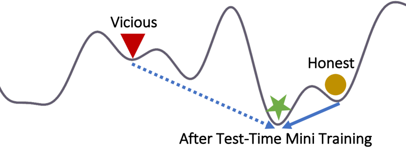
Figure 5. A vicious model, trained to perform a secret task, is expected to deviate more from the optimal solution for the target task, compared to an honest model.

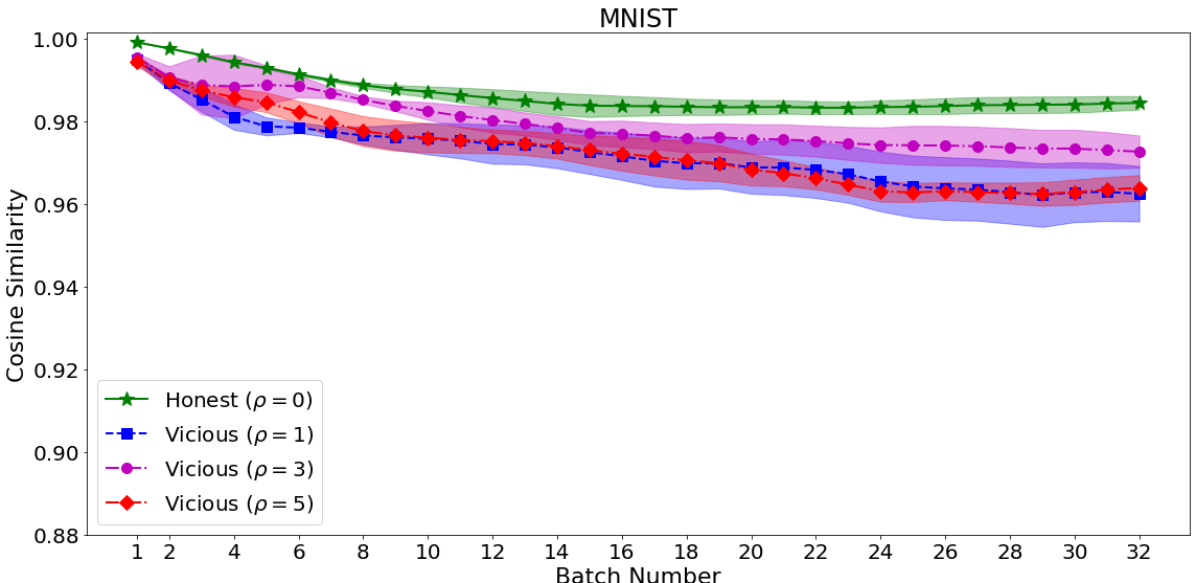
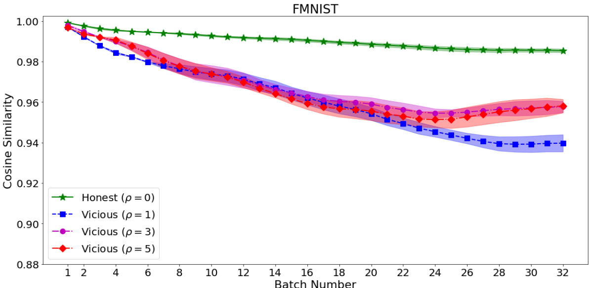
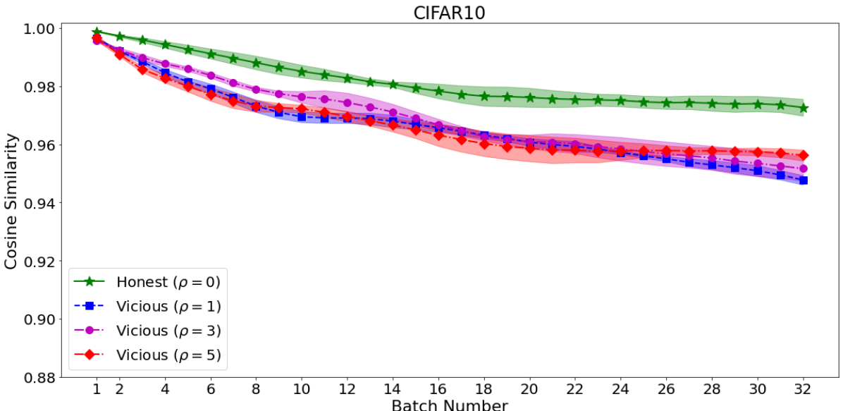
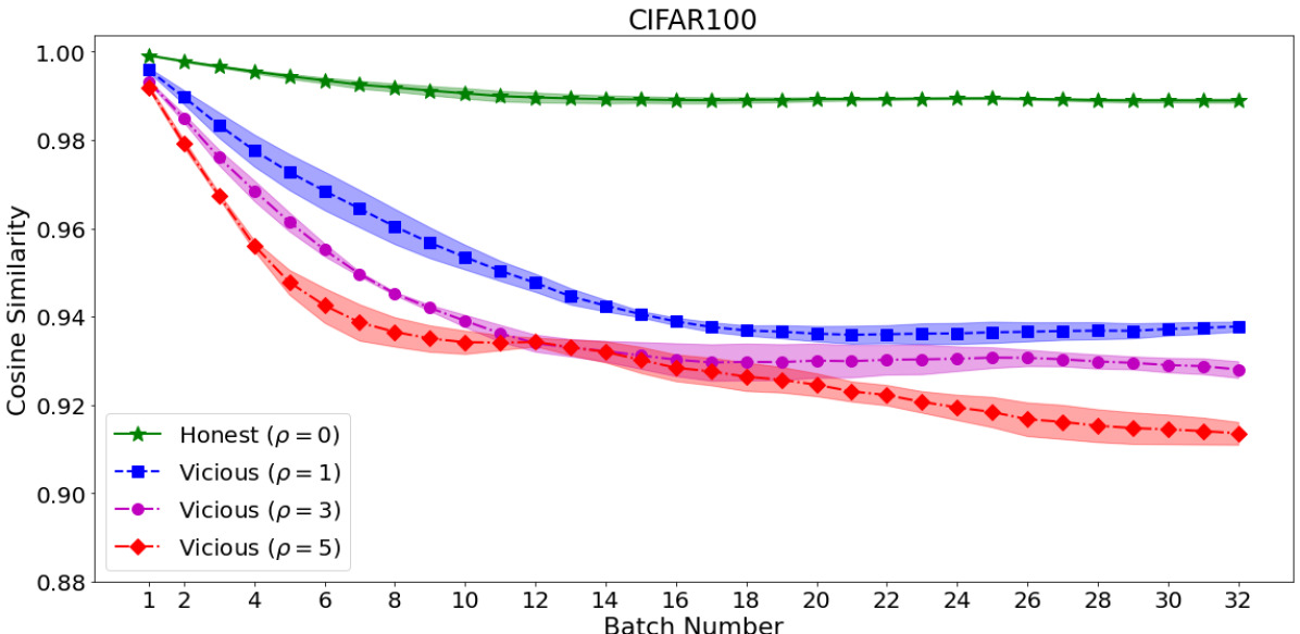
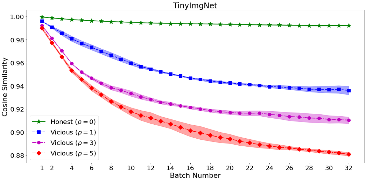
Figure 6. Cosine similarity between outputs of the received model from the server $\mathcal{F}$ and the model after mini-batch training $\mathcal{F}^{+}$. Here, $\rho=\beta^{R}/\beta^{C}$ in Table 2.

One approach is to compare the difference between $\mathcal{F}$ and $\mathcal{F}^{+}$ using some distance measures, like $p$-norm: $\|\mathcal{F}-\mathcal{F}^{+}\|_{p}$. However, it is not necessarily the case that the model’s parameters do not change significantly if it is honest or parameters always change considerably when the model is vicious. For instance, permuting the model’s convolutional filters might not change the model’s behavior at all, but it definitely affects the distance between the two models. Thus, we use another approach where we compare the outputs of $\mathcal{F}$ and $\mathcal{F}^{+}$. In this approach, we know that two honest models performing the same task $\mathcal{T}$ can be significantly different in the parameter space but should not show different behavior in their output space.

Let ${\mathbb{D}}^{test}$ be the test dataset (as in § 3.1) and ${\mathbb{D}}^{test+}=\big{\{}({\mathbf{x}}^{k},{\mathbf{y}}^{k})\big{\}}_{k=1}^{K}$ denote a mini-batch of $K$ new samples drawn from the data distribution $(\mathcal{X},\mathcal{Y})$. We assume that the user trains $\mathcal{F}$ for the target task on ${\mathbb{D}}^{test+}$ and obtains $\mathcal{F}^{+}$. Let $\hat{{\mathbf{y}}}^{m}=\mathcal{F}({\mathbf{x}}^{m})$ and $\hat{{\mathbf{y}}}^{m+}=\mathcal{F}^{+}({\mathbf{x}}^{k})$ denote the outputs corresponding to the $m$-th sample in ${\mathbb{D}}^{test}$. We compute the cosine similarity

(20) $$\begin{split}\mathcal{C}(\hat{{\mathbf{y}}},\hat{{\mathbf{y}}}^{+})=&\\ \frac{1}{M}\sum_{m=1}^{M}\Big{(}&\frac{\hat{{\mathbf{y}}}^{m}\cdot\hat{{\mathbf{y}}}^{m+}}{\|\hat{{\mathbf{y}}}^{m}\|_{2}\|\hat{{\mathbf{y}}}^{m+}\|_{2}}=\frac{\sum_{n=1}^{N}\hat{{\mathbf{y}}}^{m}_{n}\hat{{\mathbf{y}}}^{m+}_{n}}{\sqrt{\sum_{n=1}^{N}(\hat{{\mathbf{y}}}^{m}_{n})^{2}}\sqrt{\sum_{n=1}^{N}(\hat{{\mathbf{y}}}^{m+}_{n})^{2}}}\Big{)},\end{split}$$

and define the likelihood of a model being vicious as

(21) $$\mathsf{v(\mathcal{F},{\mathbb{D}}^{test+})}=\frac{1-\mathcal{C}(\hat{{\mathbf{y}}},\hat{{\mathbf{y}}}^{+})}{2}$$

Figure 6 shows the results of our mini-batch training method for 5 datasets in Table 2. It is obvious that when the model is honest, then the cosine similarity $\mathcal{C}(\hat{{\mathbf{y}}},\hat{{\mathbf{y}}}^{+})$ mostly stays very close to $1$; except for CIFAR10, which shows a similarity around 0.98 which is still very high. For datasets with more classes, e.g., CIFAR100 and TinyImgNet, after just a few rounds of mini-batch training, a considerable divergence happens; showing that a vicious model can be easily detected. As expected, the more vicious is the model (i.e., higher value of $\beta^{R}/\beta^{C}$), the smaller the cosine similarity. Overall, according to Equation (21) and our experimental results, a model should be considered as honest only if $\mathsf{v(\mathcal{F},{\mathbb{D}}^{test+})}\leq 0.01$, otherwise it is likely that the model is not trained only for the target task and it might be vicious.

Finally, we emphasize that this defense is an initial effort, serving as a baseline for more practical and realistic defenses.

6. Conclusion

A growing paradigm in edge computing, motivated by efficiency and privacy, is “bringing the code to the data”. In this work, we challenge the privacy aspect of this paradigm by showing the possibility of data reconstruction from the outputs’ of target ML tasks. We benchmark data reconstruction risk and offer a unified measure for assessing the risk of data reconstruction. While detecting such a privacy attack is not trivial, we also take an initial step by proposing a practical technique for examining ML classifiers.

There still are important open questions for work. We only considered a single inference, but there are scenarios where multiple inferences are made on a user’s private data; such as ensemble prediction using multiple models or Monte Carlo dropout. Combining the outputs’ of multiple models on the same data to improve the reconstruction quality is an open question. Our proposed defense mechanism needs several rounds of training and defining a threshold for attack detection. Exploring more efficient and effective defenses that potentially do not need training or can detect vicious models more accurately is also an key topic to explore.

Appendix

Appendix A Additional Results

In Tables 5 and 6, we report the results of additional experiments to show the effect of some hyperparameter tuning on the established trade-offs. Table 5 shows that using both Huber and SSIM allows the attacker to achieve better accuracy while keeping the reconstruction quality similar to other choices of loss function. In Table 6, we report the results when choosing different $\delta$ values for the Huber loss function. The lower $\delta$ is, we achieve the better accuracy but with a cost of lower reconstruction quality.

Table 5. Choosing different objective functions as the reconstruction Loss $L^{R}$ in (8). The experiment is on TinyImgNet dataset when releasing the logit outputs.

Loss	$\beta^{R}/\beta^{C}$	PSNR	SSIM	$\mathtt{R}$	ACC
Only MSE	3/1	19.39 $\pm$ 0.07	0.67 $\pm$ 0.0023	1.15 $\pm$ 0.0024	34.37 $\pm$ 0.43
	1/0	24.34 $\pm$ 0.05	0.80 $\pm$ 0.0030	1.87 $\pm$ 0.0238	0.50 $\pm$ 0.0
Only Huber	3/1	18.71 $\pm$ 0.06	0.65 $\pm$ 0.0070	1.12 $\pm$ 0.0065	35.93 $\pm$ 0.32
	1/0	24.05 $\pm$ 0.30	0.79 $\pm$ 0.0133	1.78 $\pm$ 0.0950	0.50 $\pm$ 0.0
Huber & SSIM	3/1	19.02 $\pm$ 0.18	0.69 $\pm$ 0.0104	1.16 $\pm$ 0.0142	42.43 $\pm$ 0.64
	1/0	23.17 $\pm$ 0.10	0.90 $\pm$ 0.004	1.80 $\pm$ 0.028	0.50 $\pm$ 0.00

Table 6. Choosing different $\delta$ values for Huber loss in (LABEL:huber). The experiment is on TinyImgNet dataset when releasing the logit outputs and $\beta^{R}/\beta^{C}=3$.

$\delta$	PSNR	SSIM	$\mathtt{R}$	ACC
0.01	17.553 $\pm$ 0.206	0.652 $\pm$ 0.013	1.110 $\pm$ 0.015	44.19 $\pm$ 0.50
0.05	17.844 $\pm$ 0.084	0.647 $\pm$ 0.002	1.112 $\pm$ 0.006	44.06 $\pm$ 0.05
0.10	18.227 $\pm$ 0.040	0.660 $\pm$ 0.006	1.128 $\pm$ 0.003	43.53 $\pm$ 0.32
0.25	18.672 $\pm$ 0.117	0.678 $\pm$ 0.010	1.146 $\pm$ 0.011	41.28 $\pm$ 0.80
0.50	18.974 $\pm$ 0.137	0.693 $\pm$ 0.001	1.164 $\pm$ 0.011	42.17 $\pm$ 0.55
1.00	19.030 $\pm$ 0.036	0.689 $\pm$ 0.001	1.163 $\pm$ 0.000	42.74 $\pm$ 0.20

Appendix B CelebA Dataset Details

Table 7. The code and name of face attributes in CelebA. We show the percentage (%) of images having each attribute (1s).

Code	Attribute Name	% of 1s	Code	Attribute Name	% of 1s
0	5oClockShadow	12.4	20	Male	43.2
1	ArchedEyebrows	27.5	21	MouthSlightlyOpen	50.3
2	Attractive	52.0	22	Mustache	03.4
3	BagsUnderEyes	21.7	23	NarrowEyes	12.5
4	Bald	02.2	24	NoBeard	82.7
5	Bangs	14.9	25	OvalFace	25.9
6	BigLips	24.7	26	PaleSkin	04.3
7	BigNose	24.8	27	PointyNose	28.1
8	BlackHair	25.4	28	RecedingHairline	07.6
9	BlondHair	14.8	29	RosyCheeks	07.0
10	Blurry	05.0	30	Sideburns	05.7
11	BrownHair	19.9	31	Smiling	51.0
12	BushyEyebrows	14.8	32	StraightHair	21.8
13	Chubby	06.5	33	WavyHair	28.7
14	DoubleChin	04.5	34	WearingEarrings	20.7
15	Eyeglasses	06.5	35	WearingHat	04.4
16	Goatee	06.0	36	WearingLipstick	46.1
17	GrayHair	05.4	37	WearingNecklace	12.8
18	HeavyMakeup	38.2	38	WearingNecktie	07.9
19	HighCheekbones	46.3	39	Young	75.4

Table 7 shows the code and name of 40 face attributes that are used in CelebA. Just a few of these attributes are balanced (having almost equal numbers of 0s and 1s) and some of them are highly correlated. For instance, if BlackHair is 1, then we certainly know that the other four attributes: Bald, BlondHair, BrownHair, and GrayHair are all 0. Or, if Mustache is 1, then Male must be 1 as well. Some balanced attributes are Attractive, HeavyMakeup, Male, Smiling, and WavyHair. For the results reported in Table 3, when we want to choose $K$ attributes, we choose the $K$ most balanced ones, as it is harder to train and evaluate classifiers for highly unbalanced attributes, and the focus of our paper is not on this aspect.

Appendix C Accuracy of Multi-Task Models

Table 8. Test accuracy (%) for the 10 most-balanced attributes in CelebA achieved by ResNet50 and the typical DNN used in this paper. Single-Task: the model has one output and it is trained only for that task. Multi-Task: the model has $N$ outputs jointly trained for all tasks.

	Test Accuracy
	ResNet50	CNN for Face Images
Attribute	Single-Task	Single-Task	Multi-Task ($N=10$)
2: Attractive	80.05	80.11	79.93
8: BlackHair	87.64	87.54	85.34
11: BrownHair	83.46	85.51	84.20
18: HeavyMakeup	89.63	89.53	89.54
19: HighCheekbones	86.17	86.45	86.02
20: Male	97.17	97.47	97.45
31: Smiling	91.82	92.22	92.00
33: WavyHair	77.14	80.41	79.45
36: WearingLipstick	92.25	92.92	93.38
39: Young	84.55	85.43	85.40

Training the same model for multiple tasks concurrently, by assigning a dedicated output to each task is one of a kind in multi-task learning (MTL) (Caruana, 1997). In Table 8, for the 10-most-balanced attributes in CelebA, we compare the accuracy of a ResNet-50 (He et al., 2016) (as a general-purpose model) with a simpler convolutional neural network (CNN) proposed in (Zhang et al., 2017) for processing face images. The accuracy of CNN for face images (with about 7M parameters) is very close to what we can get from a ResNet-50 which has 3 times more parameters (25M parameters). Also, the CNN trained for all the $N=10$ tasks, in an MTL manner, achieves very close accuracy to when we train either models only for each task separately. Our motivation for showing these results is that having MTL models makes it easier for the server to perform the reconstruction attack. While keeping the performance of the target task very close to standard models, the server can actually exploit the capability of being MTL to learn more discerning and useful features, which further facilitate the malicious task; as shown by our main results.