Structural Reductions and Stutter Sensitive Properties

Abstract.

Verification of properties expressed as $\omega$-regular languages such as LTL can benefit hugely from stutter insensitivity, using a diverse set of reduction strategies. However properties that are not stutter invariant, for instance due to the use of the neXt operator of LTL or to some form of counting in the logic, are not covered by these techniques in general.

We propose in this paper to study a weaker property than stutter insensitivity. In a stutter insensitive language both adding and removing stutter to a word does not change its acceptance, any stuttering can be abstracted away; by decomposing this equivalence relation into two implications we obtain weaker conditions. We define a shortening insensitive language where any word that stutters less than a word in the language must also belong to the language. A lengthening insensitive language has the dual property. A semi-decision procedure is then introduced to reliably prove shortening insensitive properties or deny lengthening insensitive properties while working with a reduction of a system. A reduction has the property that it can only shorten runs. Lipton’s transaction reductions or Petri net agglomerations are examples of eligible structural reduction strategies.

We also present an approach that can reason using a partition of a property language into its stutter insensitive, shortening insensitive, lengthening insensitive and length sensitive parts to still use structural reductions even when working with arbitrary properties.

An implementation and experimental evidence is provided showing most non-random properties sensitive to stutter are actually shortening or lengthening insensitive. Performance of experiments on a large (random) benchmark from the model-checking competition indicate that despite being a semi-decision procedure, the approach can still improve state of the art verification tools.

1. Introduction

Model checking is an automatic verification technique for proving the correctness of systems that have finite state abstractions. Properties can be expressed using the popular Linear-time Temporal Logic (LTL). To verify LTL properties, the automata-theoretic approach [Var07] builds a product between a Büchi automaton representing the negation of the LTL formula and the reachable state graph of the system (seen as a set of infinite runs). This approach has been used successfully to verify both hardware and software components, but it suffers from the so called "state explosion problem": as the number of state variables in the system increases, the size of the system state space grows exponentially.

One way to tackle this issue is to consider structural reductions. Structural reductions take their roots in the work of Lipton [Lip75] (with extensions by Lamport [LS89, Lam90]) and Berthelot [Ber85]. Nowadays, these reductions are still considered as an attractive way to alleviate the state explosion problem [Laa18, BLBDZ19, Thi20]. Structural reductions strive to fuse structurally "adjacent" events into a single atomic step, leading to less interleaving of independent events and less observable behaviors in the resulting system. An example of such a structural reduction is shown on Figure 1 where actions are progressively grouped (see Section 3.1 for a more detailed presentation). It can be observed that the Kripke structure representing the state space of the program is significantly simplified.

[width=]fig/fig

Figure 1. Example of reductions. (1) is a program with two threads and 3 variables. chan is a communication channel where send(int) insert a message and int recv() waits until a message is available and then consumes it. We consider that the logic only observes whether $x$ or $y$ is zero denoted $p$ and $q$. (2) depicts the state-space represented as a Kripke structure. Each node is labelled by the value of atomic propositions $p$ and $q$. When an instruction is executed the value of these propositions may evolve. (3) represents the state-space of a structurally reduced version of the program where actions of thread $\beta$ "z=40;chan.send(z)" are fused into a single atomic operation. (4) represents the state-space of a program where the three actions of the original program "z=40;chan.send(z);y=chan.recv()" are now a single atomic step.

Traditionally structural reductions construct a smaller system that preserves properties such as deadlock freedom, liveness, reachability [HP06], and stutter insensitive temporal logic [PP00] such as LTL_∖X. The verification of a stutter insensitive property on a given system does not depend on whether non observable events (i.e. that do not update atomic propositions) are abstracted or not. On Fig 1 both instructions "$z=40;$" and "$chan.send(z)$" of thread $\beta$ are non observable.

This paper shows that structural reductions can in fact be used even for fragments of LTL that are not stutter insensitive. We identify two fragments that we call shortening insensitive (if a word is in the language, any version that stutters less also) or lengthening insensitive (if a word is in the language, any version that stutters more also). Based on this classification we introduce two semi-decision procedures that provide a reliable verdict only in one direction: e.g. presence of counter examples is reliable for lengthening insensitive properties, but absence is not. We also propose to decompose properties to partition their language into stutter insensitive, shortening insensitive and lengthening insensitive parts, allowing to use structural reductions even if the property is not globally insensitive to length.

The paper is structured as follows, Section 2 presents the definitions and notations relevant to our setting in an abstract manner, focusing on the level of description of a language. Section 3 instantiates these definitions in the more concrete setting of LTL verification. Section 4 provides experimental evidence supporting the claim that the method is both applicable to many formulae and can significantly improve state of the art model-checkers. Section 5 introduces several extensions to the approach, providing new material with respect to [PPRT22]. Some related work is presented in Section 6 before concluding.

[width=0.7]fig/figure

Figure 2. $\Sigma^{\omega}$ is represented as a circle that is partitioned into equivalence classes of words ($\hat{r_{0}},\hat{r_{1}}\ldots$). Each point in the space is a word, and some of the ${\rm Phys.~{}Rev.~{}E}$ relations are represented as arrows ; the red point is the shortest word $\underline{\hat{r}}$ in the equivalence class. Gray areas are inside the language, white are outside of it. Four languages are depicted: $\mathscr{L}_{a}$: equivalence classes are entirely inside or outside a stutter insensitive language, $\mathscr{L}_{b}$: the "bottom" of an equivalence class may belong to a shortening insensitive language, $\mathscr{L}_{c}$: the "top" of an equivalence class may belong to a lengthening insensitive language, $\mathscr{L}_{d}$: some languages are neither lengthening insensitive nor shortening insensitive.

2. Definitions

In this section we first introduce in Section 2.1 a "shorter than" partial order relation on infinite words, based on the number of repetitions or stutter in the word. This partial order gives us in Section 2.2 the notions of shortening and lengthening insensitive language, which are shown to be weaker versions of classical stutter insensitivity in Section 2.3. We then define in Section 2.4 the reduction of a language which contains a shorter representative of each word in the original language. Finally we show that we can use a semi-decision procedure to verify shortening or lengthening insensitive properties using a reduction of a system.

2.1. A "Shorter than" relation for infinite words

[Word]: A word over a finite alphabet $\Sigma$ is an infinite sequence of symbols in $\Sigma$. We canonically denote a word $r$ using one of the two forms:

• (plain word) $r=a_{0}^{n_{0}}a_{1}^{n_{1}}a_{2}^{n_{2}}\ldots$ with for all $i\in{\rm Nature}$, $a_{i}\in\Sigma$, $n_{i}\in{\rm Nature}^{+}$ and $a_{i}\neq a_{i+1}$, or

• ($\omega$-word) $r=a_{0}^{n_{0}}a_{1}^{n_{1}}\ldots a_{k}^{\omega}$ with $k\in{\rm Nature}$ and for all $0\leq i\leq k$, $a_{i}\in\Sigma$, and for $i<k$, $n_{i}\in{\rm Nature}^{+}$ and $a_{i}\neq a_{i+1}$. $a_{k}^{\omega}$ represents an infinite stutter on the final symbol $a_{k}$ of the word.

The set of all words over alphabet $\Sigma$ is denoted $\Sigma^{\omega}$.

These notations using a power notation for repetitions of a symbol in a word are introduced to highlight stuttering. We force the symbols to alternate to ensure we have a canonical representation: with $\sigma$ a suffix (not starting by symbol $b$), the word $aab\sigma$ must be represented as $a^{2}b^{1}\sigma$ and not $a^{1}a^{1}b^{1}\sigma$. To represent a word of the form $aabbcccccc\ldots$ we use an $\omega$-word: $a^{2}b^{2}c^{\omega}$.

[Shorter than]: A plain word $r=a_{0}^{n_{0}}a_{1}^{n_{1}}a_{2}^{n_{2}}\ldots$ is shorter than a plain word $r^{\prime}=a_{0}^{n_{0}^{\prime}}a_{1}^{n_{1}^{\prime}}a_{2}^{n_{2}^{\prime}}\ldots$ if and only if for all $i\in{\rm Nature}$, $0<n_{i}\leq n_{i}^{\prime}$. For two $\omega$-words $r=a_{0}^{n_{0}}\ldots a_{k}^{\omega}$ and $r^{\prime}=a_{0}^{n_{0}^{\prime}}\ldots a_{k}^{\omega}$, $r$ is shorter than $r^{\prime}$ if and only if for all $i<k$, $n_{i}\leq n_{i}^{\prime}$.

We denote this relation on words as $r{\rm Phys.~{}Rev.~{}E}r^{\prime}$.

For instance, for any given suffix $\sigma$, $ab\sigma{\rm Phys.~{}Rev.~{}E}a^{2}b\sigma$. Note that $ab\sigma{\rm Phys.~{}Rev.~{}E}ab^{2}\sigma$ as well, but that $a^{2}b\sigma$ and $ab^{2}\sigma$ are incomparable. $\omega$-words are incomparable with plain words.

The ${\rm Phys.~{}Rev.~{}E}$ relation is a partial order on words.

Proof.

The relation is clearly reflexive ($\forall r\in\Sigma^{\omega},r{\rm Phys.~{}Rev.~{}E}r$), anti-symmetric ($\forall r,r^{\prime}\in\Sigma^{\omega}$, $r{\rm Phys.~{}Rev.~{}E}r^{\prime}\land r^{\prime}{\rm Phys.~{}Rev.~{}E}r\Rightarrow r=r^{\prime}$) and transitive ($\forall r,r^{\prime},r^{\prime\prime}\in\Sigma^{\omega},r{\rm Phys.~{}Rev.~{}E}r^{\prime}\land r^{\prime}{\rm Phys.~{}Rev.~{}E}r^{\prime\prime}\Rightarrow r{\rm Phys.~{}Rev.~{}E}r^{\prime\prime}$). The order is partial since some words (such as $a^{2}b\sigma$ and $ab^{2}\sigma$ presented above) are incomparable. ∎

[Stutter equivalence]: a word $r$ is stutter equivalent to $r^{\prime}$, denoted as $r\sim r^{\prime}$ if and only if there exists a shorter word $r^{\prime\prime}$ such that $r^{\prime\prime}{\rm Phys.~{}Rev.~{}E}r\land r^{\prime\prime}{\rm Phys.~{}Rev.~{}E}r^{\prime}$. This relation $\sim$ is an equivalence relation thus partitioning words of $\Sigma^{\omega}$ into equivalence classes.

We denote $\hat{r}$ the equivalence class of a word $r$ and denote $\underaccent{\bar}{\hat{r}}$ the shortest word in that equivalence class.

For any given word $r=a_{0}^{n_{0}}a_{1}^{n_{1}}a_{2}^{n_{2}}\ldots$ there is a shortest representative in $\hat{r}$ that is the word $\underaccent{\bar}{\hat{r}}=a_{0}a_{1}a_{2}\ldots$ where no symbol is ever consecutively repeated more than once (until the $\omega$ for an $\omega$-word). By definition all words that are comparable to $\underaccent{\bar}{\hat{r}}$ are stutter equivalent to each other, since $\underaccent{\bar}{\hat{r}}$ can play the role of $r^{\prime\prime}$ in the definition of stutter equivalence, giving us an equivalence relation: it is reflexive, symmetric and transitive.

For instance, with $\sigma$ denoting a suffix, $\underaccent{\bar}{\hat{r}}=ab\sigma$ would be the shortest representative of any word of $\hat{r}$ of the form $a^{n_{0}}b^{n_{1}}\sigma$. We can see by this definition that despite being incomparable, $a^{2}b\sigma\sim ab^{2}\sigma$ since $ab\sigma{\rm Phys.~{}Rev.~{}E}a^{2}b\sigma$ and $ab\sigma{\rm Phys.~{}Rev.~{}E}ab^{2}\sigma$.

2.2. Sensitivity of a language to the length of words

[Language]: a language $\mathscr{L}$ over a finite alphabet $\Sigma$ is a set of words over $\Sigma$, hence $\mathscr{L}\subseteq\Sigma^{\omega}$. We denote $\bar{\mathscr{L}}=\Sigma^{\omega}\setminus\mathscr{L}$ the complement of a language $\mathscr{L}$.

In the literature, most studies that exploit a form of stuttering are focused on stutter insensitive languages [PPH96, Val90, Pel94, GW94, HP06]. In a stutter insensitive language $\mathscr{L}$, duplicating any letter (also called stuttering) or removing any duplicate letter from a word of $\mathscr{L}$ must produce another word of $\mathscr{L}$. In other words, all stutter equivalent words in a class $\hat{r}$ must be either in the language or outside of it. Let us introduce weaker variants of this property, original in [PPRT22].

[Shortening insensitive]: a language $\mathscr{L}$ is shortening insensitive if and only if for any word $r$ it contains, all shorter words $r^{\prime}\in\Sigma^{\omega}$ such that $r^{\prime}{\rm Phys.~{}Rev.~{}E}r$ are also in $\mathscr{L}$.

For instance, a shortening insensitive language $\mathscr{L}$ that contains the word $a^{3}b\sigma$ must also contain shorter words $a^{2}b\sigma$, and $ab\sigma$. If it contains $a^{2}b^{2}\sigma$ it also contains $a^{2}b\sigma$, $ab^{2}\sigma$ and $ab\sigma$.

[Lengthening insensitive]: a language $\mathscr{L}$ is lengthening insensitive if and only if for any word $r$ it contains, all longer words $r^{\prime}\in\Sigma^{\omega}$ such that $r{\rm Phys.~{}Rev.~{}E}r^{\prime}$ are also in $\mathscr{L}$.

For instance, a lengthening insensitive language $\mathscr{L}$ that contains the word $a^{2}b\sigma$ must also contain all longer words $a^{3}b\sigma$, $a^{2}b^{2}\sigma$ …, and more generally words of the form $a^{n}b^{n^{\prime}}\sigma$ with $n\geq 2$ and $n^{\prime}\geq 1$. If it contains $\underaccent{\bar}{\hat{r}}=ab\sigma$ the shortest representative of an equivalence class, it contains all words in the stutter equivalence class.

While stutter insensitive languages have been heavily studied, there is to our knowledge no study on what reductions are possible if only one direction holds, i.e. the language is shortening or lengthening insensitive, but not both. A shortening insensitive language is essentially asking for something to happen before a certain deadline or stuttering "too much". A lengthening insensitive language is asking for something to happen at the earliest at a certain date or after having stuttered at least a certain number of times. Figure 2 represents these situations graphically.

2.3. Relationship to stutter insensitive logic

A language is both shortening and lengthening insensitive if and only if it is stutter insensitive (see Fig. 2). This fact is already used in [MD15] to identify such stutter insensitive languages using only their automaton. Furthermore since stutter equivalent classes of runs are entirely inside or outside a stutter insensitive language, a language $\mathscr{L}$ is stutter insensitive if and only if the complement language $\bar{\mathscr{L}}$ is stutter insensitive.

However, if we look at sensitivity to length and how it interacts with the complement operation, we find a dual relationship where the complement of a shortening insensitive language is lengthening insensitive and vice versa.

A language $\mathscr{L}$ is shortening insensitive if and only if the complement language $\bar{\mathscr{L}}$ is lengthening insensitive.

Proof.

Let $\mathscr{L}$ be shortening insensitive. Let $r\in\bar{\mathscr{L}}$ be a word in the complement of $\mathscr{L}$. Any word $r^{\prime}$ such that $r{\rm Phys.~{}Rev.~{}E}r^{\prime}$ must also belong to $\bar{\mathscr{L}}$, since if it belonged to the shortening insensitive $\mathscr{L}$, $r$ would also belong to $\mathscr{L}$. Hence $\bar{\mathscr{L}}$ is lengthening insensitive. The converse implication can be proved using the same reasoning. ∎

If we look at Figure 2, the dual effect of complement on the sensitivity of the language to length is apparent: if gray and white are switched we can see $\bar{\mathscr{L}_{b}}$ is lengthening insensitive and $\bar{\mathscr{L}_{c}}$ shortening insensitive.

2.4. When is visiting shorter words enough?

[Reduction] Let $I$ be a reduction function $\Sigma^{\omega}\mapsto\Sigma^{\omega}$ such that $\forall r,I(r){\rm Phys.~{}Rev.~{}E}r$. The reduction by $I$ of a language $\mathscr{L}$ is $\mathit{Red}_{I}(\mathscr{L})=\{I(r)\mid r\in\mathscr{L}\}$.

Note that the ${\rm Phys.~{}Rev.~{}E}$ partial order is not strict so that the image of a word may be the word itself, hence identity is a reduction function. In most cases however we expect the reduction function to map many words $r$ of the original language to a single shorter word $r^{\prime}$ of the reduced language. Note that given any two reduction functions $I$ and $I^{\prime}$, $\mathit{Red}_{I}(\mathit{Red}_{I^{\prime}}(\mathscr{L}))$ is still a reduction of $\mathscr{L}$. Hence chaining reduction rules still produces a reduction. As we will discuss in Section 3.1 structural reductions of a specification such as Lipton’s transaction reduction [Lip75, Laa18] or Petri net agglomerations [Ber85, Thi20] (see also Section 3.5) induce a reduction at the language level. In Fig. 1 fusing statements into a single atomic step in the program induces a reduction of the language.

Theorem 1 (Reduced Emptiness Checks).

Given two languages $\mathscr{L}$ and $\mathscr{L}^{\prime}$,

• if $\mathscr{L}$ is shortening insensitive, then $\mathscr{L}\cap\mathit{Red}_{I}(\mathscr{L}^{\prime})=\emptyset\Rightarrow\mathscr{L}\cap\mathscr{L}^{\prime}=\emptyset$

• if $\mathscr{L}$ is lengthening insensitive, then $\mathscr{L}\cap\mathit{Red}_{I}(\mathscr{L}^{\prime})\neq\emptyset\Rightarrow\mathscr{L}\cap\mathscr{L}^{\prime}\neq\emptyset$.

Proof 2.1.

(Shortening insensitive $\mathscr{L}$)$\mathscr{L}\cap\mathit{Red}_{I}(\mathscr{L}^{\prime})=\emptyset$ so there does not exists $r^{\prime}\in\mathscr{L}\cap\mathit{Red}_{I}(\mathscr{L}^{\prime})$. Because $\mathscr{L}$ is shortening insensitive, it is impossible that any run $r$ with $r^{\prime}\prec r$ belongs to $\mathscr{L}\cap\mathscr{L}^{\prime}$. (Lengthening insensitive $\mathscr{L}$) At least one word $r^{\prime}$ is in $\mathscr{L}$ and $\mathit{Red}_{I}(\mathscr{L})$. Therefore the longer word $r$ of $\mathscr{L}^{\prime}$ that $r^{\prime}$ represents is also in $\mathscr{L}$ since the language is lengthening insensitive.

With this theorem original to this paper we now can build a semi-decision procedure that is able to prove some lengthening or disprove some shortening insensitive properties using a reduction of a system.

3. Application to Verification

We now introduce the more concrete setting of LTL verification to exploit the theoretical results on languages and their shortening/lengthening sensitivity developed in Section 2.

3.1. Kripke Structure

From the point of view of LTL verification with a state-based logic, executions of a system (also called runs) are seen as infinite words over the alphabet $\Sigma=2^{\mathrm{AP}}$, where $\mathrm{AP}$ is a set of atomic propositions that may be true or false in each state. So each symbol in a run gives the truth value of all of the atomic propositions in that state of the execution, and each time an action happens we progress in the run to the next symbol. Some actions of the system update the truth value of atomic propositions, but some actions can leave them unchanged which corresponds to stuttering.

[Kripke Structure Syntax] Let $\mathrm{AP}$ designate a set of atomic propositions. A Kripke structure $\mathit{KS}_{\mathrm{AP}}=\langle S,R,\lambda,s_{0}\rangle$ over $\mathrm{AP}$ is a tuple where $S$ is the set of states, $R\subseteq S\times S$ is the transition relation, $\lambda:S\mapsto 2^{\mathrm{AP}}$ is the state labeling function, and $s_{0}\in S$ is the initial state. [Kripke Structure Semantics] The language $\mathscr{L}(\mathit{KS}_{\mathrm{AP}})$ of a Kripke structure $\mathit{KS}_{\mathrm{AP}}$ is defined over the alphabet $2^{\mathrm{AP}}$. It contains all runs of the form $r=\lambda(s_{0})\lambda(s_{1})\lambda(s_{2})\ldots$ where $s_{0}$ is the initial state of $\mathit{KS}_{\mathrm{AP}}$ and $\forall i\in{\rm Nature}$, either $(s_{i},s_{i+1})\in R$, or if $s_{i}$ is a deadlock state such that $\forall s^{\prime}\in S,(s_{i},s^{\prime})\not\in R$ then $s_{i+1}=s_{i}$.

All system executions are considered maximal, so that they are represented by infinite runs. If the system can deadlock or terminate in some way, we can extend these finite words by an $\omega$ stutter on the last symbol of the word to obtain a run.

Example. Subfigure (1) of Figure 1 depicts a program where each thread ($\alpha$ and $\beta$) has three reachable positions (we consider that each instruction is atomic). In this example we consider that the logic only observes two atomic propositions $p$ (true when $x=0$) and $q$ (true when $y=0$). The variable $z$ is not observed.

Subfigure (2) of Figure 1 depicts the reachable states of this system as a Kripke structure. Actions of thread $\beta$ (which do not modify the value of $p$ or $q$) are horizontal while actions of thread $\alpha$ are vertical. While each thread has 3 reachable positions, the emission of the message by $\beta$ must precede the reception by $\alpha$ so that some situations are unreachable. Based on Definition 3.1 that extends by an infinite stutter runs that end in a deadlock, we can compute the language $\mathscr{L}_{A}$ of this system. It consists in three parts: when thread $\beta$ goes first $pq^{3}$ $\bar{p}q$ $\bar{p}\bar{q}^{\omega}$, with an interleaving $pq^{2}$ $\bar{p}q^{2}$ $\bar{p}\bar{q}^{\omega}$, and when thread $\alpha$ goes first $pq$ $\bar{p}q^{3}$ $\bar{p}\bar{q}^{\omega}$.

In subfigure (3) of Figure 1, the actions "$z=40;chan.send(z);$"of thread $\beta$ are fused into a single atomic operation. This is possible because action $z=40$ of thread $\beta$ is stuttering (it cannot affect either $p$ or $q$) and is non-interfering with other events (it neither enables nor disables any event other than subsequent instruction "chan.send(z)"). The language of this smaller KS is a reduction of the language of the original system. It contains two runs: thread $\alpha$ goes first $pq$ $\bar{p}q^{2}$ $\bar{p}\bar{q}^{\omega}$ and thread $\beta$ goes first $pq^{2}$ $\bar{p}q$ $\bar{p}\bar{q}^{\omega}$.

In subfigure (4) of Figure 1, the already fused action "$z=40;chan.send(z);$"of thread $\beta$ is further fused with the chan.recv(); action of thread $\alpha$. This leads to a smaller KS whose language is still a reduction of the original system now containing a single run: $pq$ $\bar{p}q$ $\bar{p}\bar{q}^{\omega}$. This simple example shows the power of structural reductions when they are applicable, with a drastic reduction of the initial language.

3.2. Automata theoretic verification

Let us consider the problem of model-checking of an $\omega$-regular property $\varphi$ (such as LTL) on a system using the automata-theoretic approach [Var07]. In this approach, we wish to answer the problem of language inclusion: do all runs of the system $\mathscr{L}(\mathit{KS})$ belong to the language of the property $\mathscr{L}(\varphi)$ ? To do this, when the property $\varphi$ is an omega-regular language (e.g. an LTL or PSL formula), we first negate the property $\lnot\varphi$, then build a (variant of) a Büchi automaton $A_{\lnot\varphi}$ whose language consists of runs that are not in the property language $\mathscr{L}(A_{\lnot\varphi})=\Sigma^{\omega}\setminus\mathscr{L}(\varphi)$. We then perform a synchronized product between this Büchi automaton and the Kripke structure $\mathit{KS}$ corresponding to the system’s state space $A_{\lnot\varphi}\otimes\mathit{KS}$ (where $\otimes$ is defined to satisfy $\mathscr{L}(A\otimes B)=\mathscr{L}(A)\cap\mathscr{L}(B)$). Either the language of the product is empty $\mathscr{L}(A_{\lnot\varphi}\otimes\mathit{KS})=\emptyset$, and the property $\varphi$ is thus true of this system, or the product is non empty, and from any run in the language of the product we can build a counter-example to the property.

We will consider in the rest of the paper that the shortening or lengthening insensitive language of definitions 2.2 and 2.2 is given as an omega-regular language or Büchi automaton typically obtained from the negation of an LTL property, and that the reduction of definition 2.4 is applied to a language that corresponds to all runs in a Kripke structure typically capturing the state space of a system.

LTL verification with reductions. With theorem 1, a shortening insensitive property shown to be true on the reduction (empty intersection with the language of the negation of the property) is also true of the original system. A lengthening insensitive property shown to be false on the reduction (non-empty intersection with the language of the negation of the property, hence counter-examples exist) is also false in the original system. Unfortunately, our procedure cannot prove using a reduction that a shortening insensitive property is false, or that a lengthening insensitive property is true. We offer a semi-decision procedure.

3.3. Detection of language sensitivity

We now present a strategy to decide if a given property expressed as a Büchi automaton is shortening insensitive, lengthening insensitive, or both.

This section relies heavily on the operations introduced and discussed at length in [MD15]. The authors define two syntactic transformations $sl$ and $cl$ of a transition-based generalized Büchi automaton (TGBA) $A_{\varphi}$ that can be built from any LTL formula $\varphi$ to represent its language $\mathscr{L}(\varphi)=\mathscr{L}(A_{\varphi})$ [Cou99]. TGBA are a variant of Büchi automata where the acceptance conditions are placed on edges rather than states of the automaton.

The $cl$ closure operation decreases stutter, it adds to the language any word $r^{\prime}\in\Sigma^{\omega}$ that is shorter than a word $r$ in the language. Informally, the strategy consists in detecting when a sequence $q_{1}\xrightarrow{a}q_{2}\xrightarrow{a}q_{3}$ is possible and adding an edge $q_{1}\xrightarrow{a}q_{3}$, hence its name $cl$ for "closure". The $sl$ self-loopization operation increases stutter, it adds to the language any run $r^{\prime}\in\Sigma^{\omega}$ that is longer than a run $r$ in the language. Informally, the strategy consists in adding a self-loop to any state so that we can always decide to repeat a letter (and stay in that state) rather than progress in the automaton, hence its name $sl$ for "self-loop". More formally $\mathscr{L}(cl(A_{\varphi}))=\{r^{\prime}\mid\exists r\in\mathscr{L}(A_{\varphi}),r^{\prime}{\rm Phys.~{}Rev.~{}E}r\}$ and $\mathscr{L}(sl(A_{\varphi}))=\{r^{\prime}\mid\exists r\in\mathscr{L}(A_{\varphi}),r{\rm Phys.~{}Rev.~{}E}r^{\prime}\}$.

Using these operations [MD15] shows that there are several possible ways to test if an omega-regular language (encoded as a Büchi automaton) is stutter insensitive: essentially applying either of the operations $cl$ or $sl$ should leave the language unchanged. This allows to recognize that a property is stutter insensitive even though it syntactically contains e.g. the neXt operator of LTL.

For instance $A_{\varphi}$ is stutter insensitive if and only if $\mathscr{L}(sl(cl(A_{\varphi}))\otimes A_{\lnot\varphi})=\emptyset$. The full test is thus simply reduced to a language emptiness check testing that both $sl$ and $cl$ operations leave the language of the automaton unchanged.

Indeed for stutter insensitive languages, all or none of the runs belonging to a given stutter equivalence class of runs $\hat{r}$ must belong to the language $\mathscr{L}(A_{\varphi})$. In other words, if shortening or lengthening a run can make it switch from belonging to $A_{\varphi}$ to belonging to $A_{\lnot\varphi}$, the language is stutter sensitive. This is apparent on Figure 2.

We want weaker conditions here, but we can reuse the $sl$ and $cl$ operations developed for testing stutter insensitivity. Indeed for an automaton $A$ encoding a shortening insensitive language, $\mathscr{L}(cl(A))=\mathscr{L}(A)$ should hold. Conversely if $A$ encodes a lengthening insensitive language, $\mathscr{L}(sl(A))=\mathscr{L}(A)$ should hold. We express these tests as emptiness checks on a product in the following way.

Theorem 2 (Testing sensitivity).

Let $A$ designate a Büchi automaton, and $\bar{A}$ designate its complement.

$\mathscr{L}(cl(A)\otimes\bar{A})=\emptyset$, if and only if $A$ defines a shortening insensitive language.

$\mathscr{L}(sl(A)\otimes\bar{A})=\emptyset$ if and only if $A$ defines a lengthening insensitive language.

Proof 3.1.

The expression $\mathscr{L}(cl(A)\otimes\bar{A})=\emptyset$ is equivalent to $\mathscr{L}(cl(A))=\mathscr{L}(A)$. The lengthening insensitive case is similar.

Thanks to property 2.3, and in the spirit of [MD15] we could also test the complement of a language for the dual property if that is more efficient, i.e. $\mathscr{L}(sl(\bar{A})\otimes A)=\emptyset$ if and only if $A$ defines a shortening insensitive language and similarly $\mathscr{L}(cl(\bar{A})\otimes A)=\emptyset$ iff $A$ is lengthening insensitive. We did not really investigate these alternatives as the complexity of the test was already negligible in all of our experiments.

3.4. Agglomeration of events produces shorter runs

Among the possible strategies to reduce the complexity of analyzing a system are structural reductions. Depending on the input formalism the terminology used is different, but the main results remain stable.

In [Lip75] transaction reduction consists in fusing two adjacent actions of a thread (or even across threads in recent versions such as [Laa18] ). The first action must not modify atomic properties and must be commutative with any action of other threads. Fusing these actions leads to shorter runs, where a stutter is lost. In the program of Fig. 1, "z=40" is enabled from the initial state and must happen before "chan.send(z)", but it commutes with instructions of thread $\alpha$ and is not observable. Hence the language $\mathscr{L}_{B}$ built with an atomic assumption on "z=40;chan.send(z)" is indeed a reduction of $\mathscr{L}_{A}$.

Let us reason at the level of a Kripke structure. The goal of such reductions is to structurally detect the following situation in language $\mathscr{L}$: let $r=a_{0}^{n_{0}}a_{1}^{n_{1}}a_{2}^{n_{2}}\ldots$ designate a run (not necessarily in the language), there must exist two indexes $i$ and $j$ such that for any natural number $k$, $i\leq k\leq j$, $r_{k}=a_{0}^{n_{0}}\ldots a_{i}^{n_{i}}\ldots a_{k}^{n_{k}+1}\ldots a_{j}^{n_{j}}\ldots$ is in the language. In other words, the set of runs described as: $\{r_{k}=a_{0}^{n_{0}}\ldots a_{i}^{n_{i}}\ldots a_{k}^{n_{k}+1}\ldots a_{j}^{n_{j}}\ldots\mid i\leq k\leq j\}$ must belong to the language. This corresponds to an event that does not impact the truth value of atomic propositions (it stutters) and can be freely commuted with any event that occurs between indexes $i$ and $j$ in the run. This event is simply constrained to occur at the earliest at index $i$ in the run and at the latest at index $j$. In Fig 1 the event "z=40" can happen as early as in the initial state, and must occur before "chan.send(z)" and thus matches this definition.

Note that these runs are all stutter equivalent, but are incomparable by the shorter than relation (e.g. $aabc\sigma,abbc\sigma,abcc\sigma$ are incomparable). In this situation, a reduction can choose to only represent the run $r$ (e.g. $r=abc\sigma$ represents all these runs) instead of any of these runs. This run was not originally in the language in general, but it is indeed shorter than any of the $r_{k}$ runs so it matches definition 2.4 for a reduction. Note that the stutter-equivalent class $\hat{r}$ of $r$ does contain all these longer runs so that in a stutter insensitive context, examining $r$ is enough to conclude for any of the runs in $\hat{r}$. This is why usage of structural reductions is compatible with verification of a logic such as $LTL_{\setminus X}$ and has been proposed for that express purpose in the literature [PP00, HP06, Laa18].

Thus transaction reductions [Lip75, Laa18] as well as both pre-agglomeration and post-agglomeration of Petri nets [PP00, EHP05, HP06, Thi20] produce a system whose language is a reduction of the language of the original system.

A formal definition involves a) introducing the syntax of a formalism and b) its semantics in terms of language, then c) defining the reduction rule, and d) proving its effect is a reduction at the language level. The exercise is not particularly difficult, and the definition of reduction rules mostly fall into the category above, where a non observable event that happens at the earliest at point $i$ in the run and at the latest at point $j$ in the run is abstracted from the trace. As an example, we provide in Section 3.5 such a proof for structural agglomerations rules on Petri nets.

Our experimental Section 4.2 uses slightly extended versions of these rules (defined in [Thi20]) for (potentially partial) pre and post-agglomeration. That paper presents $22$ structural reductions rules from which we selected the rules valid in the context of LTL verification. Only one rule preserving stutter insensitive LTL was not compatible with our approach since it does not produce a reduction at the language level: rule $3$ "Redundant transitions" proposes that if two transitions $t_{1}$ and $t_{2}$ have the same combined effect as a transition $t$, and firing $t_{1}$ enables $t_{2}$, $t$ can be discarded from the net. This reduces the number of edges in the underlying $\mathit{KS}$ representing the state space, but does not affect reachability of states. However, it selects as representative a run involving both $t_{1}$ and $t_{2}$ that is longer than the one using $t$ in the original net, it is thus not legitimate to use in our strategy (although it remains valid for $LTL_{\setminus X}$). Rules $14$ "Pre agglomeration" and $15$ "Post agglomeration" are the most powerful rules of [Thi20] that we are able to apply in our context. They are known to preserve $LTL_{\setminus X}$ (but not full LTL) and their effect is a reduction at the language level, hence we can use them when dealing with shortening/lengthening insensitive formulae.

3.5. Petri net agglomeration rules

This section presents agglomeration rules for Petri net, and shows that this transformation of the structure of the net leads to a reduction of the associated language in the sense of definition 2.4. All of this section is new content with respect to [PPRT22].

Structure. A Petri net $N=\langle\mathcal{P},\mathcal{T},\mathcal{W}_{-},\mathcal{W}_{+},m_{0}\rangle$ is a tuple where $\mathcal{P}$ is the finite set of places, $\mathcal{T}$ is the finite set of transitions, $\mathcal{W}_{-}:\mathcal{P}\times\mathcal{T}\mapsto{\rm Nature}$ and $\mathcal{W}_{+}:\mathcal{P}\times\mathcal{T}\mapsto{\rm Nature}$ represent the pre and post incidence matrices, and $m_{0}:\mathcal{P}\mapsto{\rm Nature}$ is the initial marking.

Notations: We use $p$ (resp. $t$) to designate a place (resp. transition) or its index dependent on the context. We let markings $m$ be manipulated as vectors of natural with $|\mathcal{P}|$ entries. We let $\mathcal{W}_{-}(t)$ and $\mathcal{W}_{+}(t)$ for any given transition $t$ represent vectors with $|\mathcal{P}|$ entries. In vector spaces, we use $v\geq v^{\prime}$ to denote $\forall i,v(i)\geq v^{\prime}(i)$, and we use sum $v+v^{\prime}$ with the usual element-wise definition. Since a Petri net is bipartite graph, we note $\bullet{n}$ (resp. ${n}\bullet$) the pre set (resp. post set) of a node $n$ (place or transition). E.g. for a place $p$ its pre set is $\bullet{p}=\{t\in\mathcal{T}{}\mid\mathcal{W}_{+}(p,t)>0\}$.

Semantics. The semantics of a Petri net are given by the firing rule $\xrightarrow{t}$ that relates pairs of markings: in any marking $m\in{\rm Nature}^{|\mathcal{P}|}$, if $t\in\mathcal{T}$ satisfies $m\geq\mathcal{W}_{-}(t)$, then $m\xrightarrow{t}m^{\prime}$ with $m^{\prime}=m+\mathcal{W}_{+}(t)-\mathcal{W}_{-}(t)$. Given a set of atomic propositions $\mathrm{AP}$ and an evaluation function $\lambda:{\rm Nature}^{|\mathcal{P}|}\mapsto 2^{\mathrm{AP}}$, we can associate to a net $N=\langle\mathcal{P},\mathcal{T},\mathcal{W}_{-},\mathcal{W}_{+},m_{0}\rangle$ the corresponding Kripke structure $\mathit{KS}_{\mathrm{AP}}=\langle S={\rm Nature}^{|\mathcal{P}|},R=\{(m,m^{\prime})\mid\exists t\in\mathcal{T},m\xrightarrow{t}m^{\prime}\},\lambda,s_{0}=m_{0}\rangle$ over $\mathrm{AP}$.

We suppose that an atomic proposition is a Boolean formula (using $\lor,\land,\lnot$) of comparisons ($\bowtie\in\{<,\leq,=,\geq,>\}$) of arbitrary weighted sum of place markings to another sum or a constant, e.g. $\sum_{p\in\mathcal{P}}\alpha_{p}\cdot m(p)\bowtie k$, with $\alpha_{p}\in\mathds{Z}$ and $k\in\mathds{Z}$. The support of a property expressed over $\mathrm{AP}$ is the set of places whose marking is truly used in an atomic predicate, i.e. such that at least one comparison atom has a non zero $\alpha_{p}$ in a sum. The support $\mathit{Supp}\subseteq\mathcal{P}{}$ of the property defines the subset $\mathit{Inv}_{\mathrm{AP}}{}\subseteq\mathcal{T}$ of invisible or stuttering transitions $t$ satisfying $\forall p\in\mathit{Supp},\mathcal{W}_{-}(p,t)=\mathcal{W}_{+}(p,t)$. Hence, given a labeling function $\lambda:{\rm Nature}^{\mathcal{P}}{}\mapsto 2^{\mathrm{AP}}$, we can guarantee that $\forall t\in\mathit{Inv}_{\mathrm{AP}}{}$ and any $m,m^{\prime}\in{\rm Nature}^{\mathcal{P}}{}$, if $m\xrightarrow{t}m^{\prime}$ then $\lambda(m)=\lambda(m^{\prime})$. With respect to stutter, the atomic propositions $\mathrm{AP}$ are only interested in the projection of reachable markings over the variables in the support, values of places in $\mathcal{P}{}\setminus\mathit{Supp}$ are not observable in markings. A small support means more potential reductions, as rules mostly cannot apply to observed places or their neighborhood.

Agglomeration in a place $p$ consists in discarding $p$ and its surrounding transitions (pre and post set of $p$) to build instead a transition for every element in the Cartesian product $\bullet{p}\times{p}\bullet$ that represents the effect of the sequence of firing a transition in $\bullet{p}$ then immediately a transition in ${p}\bullet$. This "acceleration" of tokens in $p$ reduces interleaving in the state space, but can preserve properties of interest if $p$ is chosen correctly. This type of reduction has been heavily studied [HP06, Laa18] as it forms a common ground between structural reductions, partial order reductions and techniques that stem from transaction reduction.

We present here two rules that can be used to safely decide if a place can be agglomerated. Figure 3 shows these rules graphically, using the classical graphical notation for Petri nets.

Pre and Post Agglomeration. Let $N$ designate a Petri net and $\mathit{Supp}\subseteq\mathcal{P}{}$ be the support of a property on this net. Let $p\in\mathcal{P}$ be a place of $N$ satisfying:

$p\in\mathcal{P}\setminus\mathit{Supp}$	$p$ not in support
$m_{0}(p)=0$	initially unmarked
$\bullet{p}\cap{p}\bullet=\emptyset$	distinct feeders and consumers
$\forall h\in\bullet{p},\mathcal{W}_{-}(p,h)=1$	feeders produce a single token in $p$
$\forall f\in{p}\bullet,\mathcal{W}_{+}(p,f)=1$	consumers require a single token in $p$

Pre agglomeration in $p$ is possible if it also the case that:

$\forall h\in\bullet{p},$
	$\left\{\begin{array}[]{@{}ll@{}}h\in\mathit{Inv}_{\mathrm{AP}}{}&$feeders are stuttering $\\ {h}\bullet=\{p\}&p$ is the single output of $h\\ \exists p_{1}\in\bullet{h},\mathcal{W}_{+}(p_{1},h)<\mathcal{W}_{-}(p_{1},h)&h$ is divergent free$\\ \forall p_{2}\in\bullet{h},{p_{2}}\bullet=\{h\}&h$ is strongly quasi-persistent$\\ \end{array}\right.$

Post agglomeration in $p$ is possible if it also the case that:

$\forall f\in{p}\bullet,$
	$\left\{\begin{array}[]{@{}ll@{}}f\in\mathit{Inv}_{\mathrm{AP}}{}&$all consumers are stuttering $\\ \bullet{f}=\{p\}&$no other inputs to $f$ $\\ \end{array}\right.$

In either of these cases, we agglomerate place $p$ leading to a net where

• we discard all transitions in $\bullet{p}\cup{p}\bullet$ and place $p$ from the net, and

• $\forall h\in\bullet{p},\forall f\in{p}\bullet,$ we add a new transition $t$ such that $\mathcal{W}_{-}(t)=\mathcal{W}_{-}(h)+\mathcal{W}_{-}(f)$ and $\mathcal{W}_{+}(t)=\mathcal{W}_{+}(h)+\mathcal{W}_{+}(f)$

Pre agglomeration (see Fig. 3(a)) looks for a place $p$ such that all predecessor transitions $h\in\bullet{p}$ are stuttering, have $p$ as single output place, and once enabled cannot be disabled by firing any other transition (hence they commute freely with other transitions that do not consume in $p$). With these conditions, we can always "delay" the firing of $h$ until it becomes relevant to enable a transition that consumes from $p$. This will yield a Petri net whose language is a reduction of the original one.

Conversely, Post agglomeration (see Fig. 3(b)) looks for a place $p$ such that all successor transitions $f\in{p}\bullet$ are stuttering, and have $p$ as single input place. With these conditions, tokens that arrive in $p$ are always free to choose where they want to go, and nothing can prevent them from going there. Instead of waiting in $p$ until we take this decision, we can make this choice immediately after firing a transition $h$ that places a token in $p$. This again will yield a Petri net whose language is a reduction of the original one.

[width=.48]fig/preagglo1 [width=.48]fig/preagglo2

(a) Pre-agglomeration. The firing of transition $h$ that is stuttering in a run can be delayed until an $f$ transition is fired. The $h$ transition is a right-mover in transaction reduction terms.

[width=.48]fig/postagglo1 [width=.48]fig/postagglo2

(b) Post-agglomeration. The firing of transition $f$ that is stuttering in a run can be advanced to immediately after the $h$ transition is fired. The $f$ transition is a left-mover in transaction reduction terms.

Figure 3. Pre and Post agglomeration rules, graphically represented. Figures to the left are before agglomeration and to the right after the transformation. Places in red cannot be part of the support of the property.

Let $N$ be a Petri net, and $p$ a place of this net satisfying one of the agglomeration criterion. The agglomeration in $p$ of $N$ produces a net whose language is a reduction of the language of $N$.

Proof 3.2.

(Sketch of) Consider an execution of $N$ of the form: $m_{0}\xrightarrow{t_{0}}\ldots m_{i}\xrightarrow{h}m_{i+1}\xrightarrow{t_{i+1}}\ldots m_{j}\xrightarrow{f}m_{j+1}\ldots$ where $h\in\bullet{p}$, $f\in{p}\bullet$ and $\forall k\in{\rm Nature},i<k<j$, $t_{k}\not\in\bullet{p}\cup{p}\bullet$. For pre-agglomeration of $N$ in $p$, the image of this execution in the agglomerated net is of the form: $m_{0}\xrightarrow{t_{0}}\ldots m_{i}\xrightarrow{t_{i+1}}m_{i+1}^{\prime}\ldots m_{j}^{\prime}\xrightarrow{h.f}m_{j+1}\ldots$ where the firing of $h$ has shifted to the right until it is fused with the subsequent firing of $f$. Indeed, we have the strong diamond property that states commutativity of $h$ with any of the transitions between $h$ and $f$ in the execution. Let $t$ be such a transition, if $\exists m,m1,m^{\prime}\in{\rm Nature}^{\mathcal{P}}{}$ such that $m\xrightarrow{h}m_{1}\xrightarrow{t}m^{\prime}$ then $\exists m_{2},m\xrightarrow{t}m_{2}\xrightarrow{h}m^{\prime}$. Indeed $h$ cannot be disabled by any transition once it is enabled (due to "strongly quasi persistent" property), and firing of $h$ cannot enable any transition not in ${p}\bullet$ (since ${h}\bullet=\{p\}$). The semantics of a Petri net also induce that firing $h$ before or after $t$ lead to the same marking. Furthermore, the underlying run in the agglomerated net is shorter (by one repetition) than the original run, because $h$ is guaranteed to stutter (it is one of the constraints that $h\in\mathit{Inv}_{\mathrm{AP}}{}$).

If the execution of the original net contains a firing of transition $h$ but not of $f$, $m_{0}\xrightarrow{t_{0}}\ldots m_{i}\xrightarrow{h}m_{i+1}\ldots$ where $h\in\bullet{p}$, and $\forall k\in{\rm Nature},k>i$, $t_{k}\not\in{p}\bullet$, the image is the execution $m_{0}\xrightarrow{t_{0}}\ldots m_{i}\xrightarrow{t_{i+1}}m_{i+1}^{\prime}\ldots$ where the transition $h$ is never fired. Since $h$ is stuttering, this corresponding run is shorter than the original (by one repetition).

If the execution does not contain any firing of a transition in $\bullet{p}\cup{p}\bullet$, the image of the execution is the execution itself which is legitimate since identity is a reduction. Lastly, the divergent free constraint ensures that $h$ cannot be fired infinitely many times in succession so that the original net cannot exhibit an execution of the form $m_{0}\ldots m^{\prime}\xrightarrow{h}m^{\prime\prime}\xrightarrow{h}\ldots$ (ending on infinitely many firings of $h$) that would no longer exist in the agglomerated net.

A similar reasoning is possible for post agglomeration, given an execution $m_{0}\xrightarrow{t_{0}}\ldots m_{i}\xrightarrow{h}m_{i+1}\xrightarrow{t_{i+1}}\ldots m_{j}\xrightarrow{f}m_{j+1}\ldots$ where $h\in\bullet{p}$, $f\in{p}\bullet$ and $\forall k\in{\rm Nature},i<k<j$, $t_{k}\not\in\bullet{p}\cup{p}\bullet$ of the original net, the image in the agglomerated net is $m_{0}\xrightarrow{t_{0}}\ldots m_{i}\xrightarrow{h.f}m_{i+1}^{\prime}\xrightarrow{t_{i+1}}\ldots$ where the firing of $f$ has shifted to the left until it is fused with the preceding firing of $h$. Again the diamond property applies, $f$ is enabled as soon as $h$ fires and cannot subsequently be disabled by other transitions. Because $f$ is constrained to be stuttering, the corresponding run is shorter than the original one.

The pre and post agglomeration rules presented here are variants on the rules initially introduced by Berthelot [Ber85], and have been used in the context of stutter insensitive LTL model-checking [PP00, HP06].

4. Experimentation

4.1. A Study of Properties

This section provides an empirical study of the applicability of the techniques presented in this paper to LTL properties found in the literature. To achieve this we explored several LTL benchmarks [EH00, SB00, DAC98, HJM⁺21, KBG⁺21]. Some work [EH00, SB00] summarizes the typical properties that users express in LTL. The formulae of this benchmark have been extracted directly from the literature. Dwyer et al. [DAC98] proposes property specification patterns, expressed in several logics including LTL. These patterns have been extracted by analysing 447 formulae coming from real world projects. The RERS challenge [HJM⁺21] presents generated formulae inspired from real world reactive systems. The MCC [KBG⁺21] benchmark establishes a huge database of $45152$ LTL formulae in the form of $1411$ Petri net models coming from $114$ origins with for each one $32$ random LTL formulae. These formulae use up to $5$ state-based atomic propositions, limit the nesting depth of temporal operators to $5$ and are filtered in order to be non trivial. Since these formulae come with a concrete system we were able to use this benchmark to also provide performance results for our approach in Section 4.2. We retained $43989$ model/formula pairs from this benchmark, the missing $1163$ were rejected due to parse limitations of our tool when the model size is excessive ($>10^{7}$ transitions). This set of roughly 2200 human-like formulae and 44k random ones lets us evaluate if the fragment of LTL that we consider is common in practice. Table 1 summarizes, for each benchmark, the number and percentage of formulae that are either stuttering insensitive, lengthening insensitive, or shortening insensitive. The sum of both shortening and lengthening formulae represents more than one third (and up to 60 percent) of the formulae of these benchmarks.

Concerning the polarity, although lengthening insensitive formulae seem to appear more frequently, most of these benchmarks actually contain each formula in both positive and negative forms (we retained only one) so that the summed percentage might be more relevant as a metric since lengthening insensitivity of $\varphi$ is equivalent to shortening insensitivity of $\lnot\varphi$. Analysis of the human-like Dwyer patterns [DAC98] reveals that shortening/lengthening insensitive formulae mostly come from the patterns precedence chain, response chain and constrained chain. These properties specify causal relation between events, that are observable as causal relations between observably different states (that might be required to strictly follow each other), but this causality chain is not impacted by non observable events.

Benchmark	Total	SI	LI	ShI	LS
Dwyer et al. [DAC98]	55	32 (58%)	13 (23%)	9 (16%)	1 (1.81%)
Spot [EH00, DAC98, SB00]	94	63 (67%)	17 (18%)	11 (1%)	3 (3%)
RERS [HJM+21].	2050	714 (35%)	777 (38%)	559 (28%)	0
MCC [KBG+21]	43989	24462 (56%)	6837 (14%)	5390 (12%)	7300 (16%)

Table 1. Sensitivity to length of properties measured using several LTL benchmarks. We distinguish stutter insensitive (SI), lengthening insensitive (LI), shortening insensitive (ShI), and length sensitive (LS) formulae.

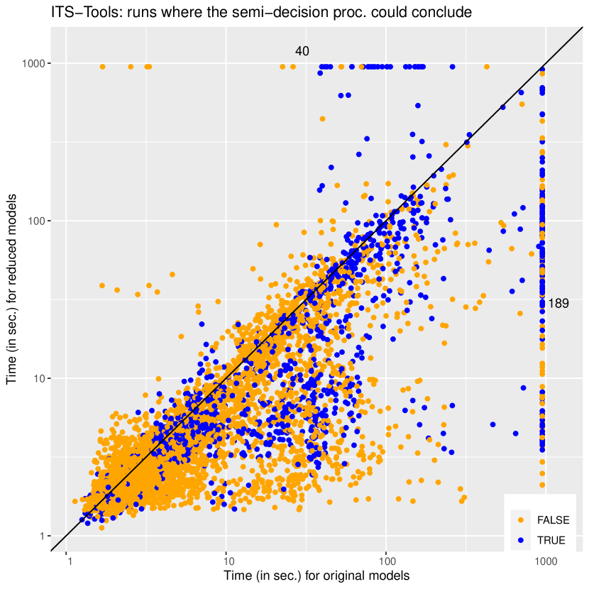
(a) ITS-tools on decidable instances

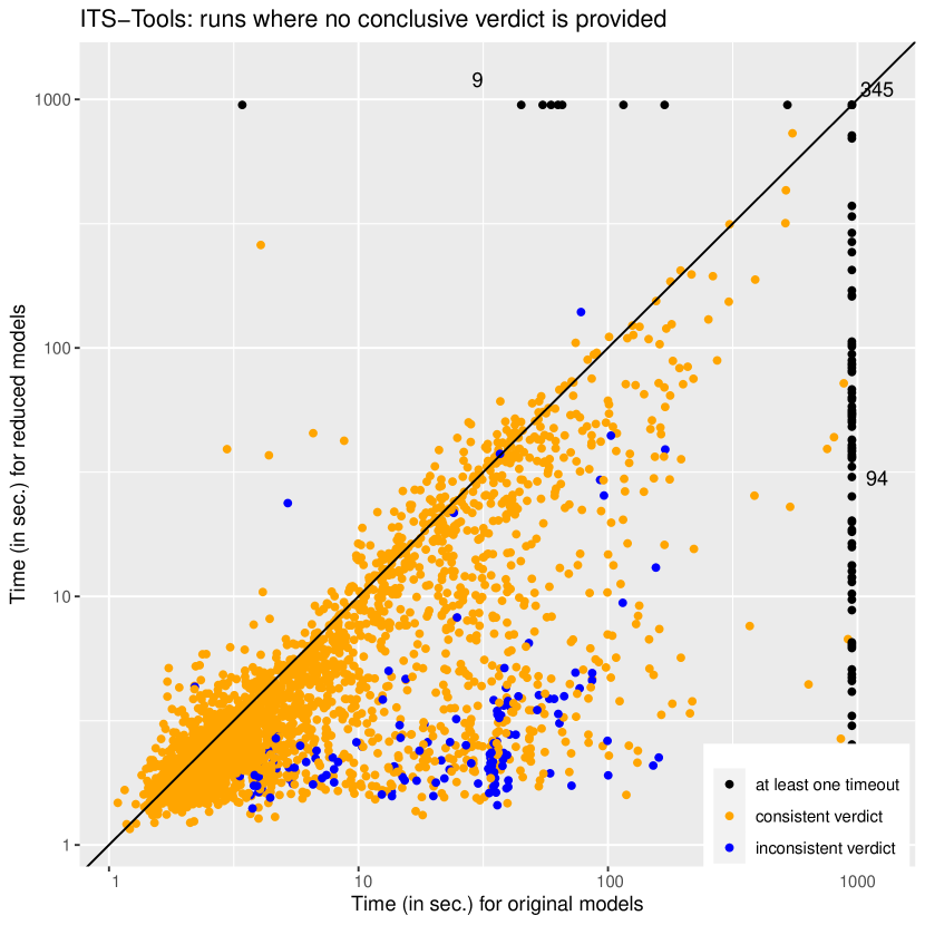
(b) ITS-tools on non decidable instances

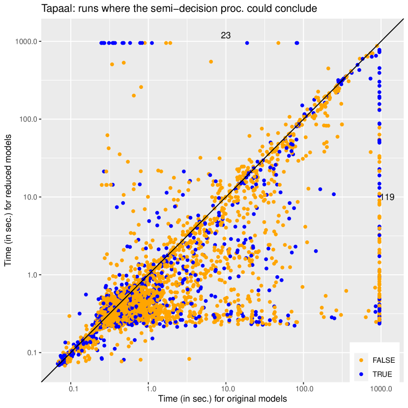
(c) Tapaal on decidable instances

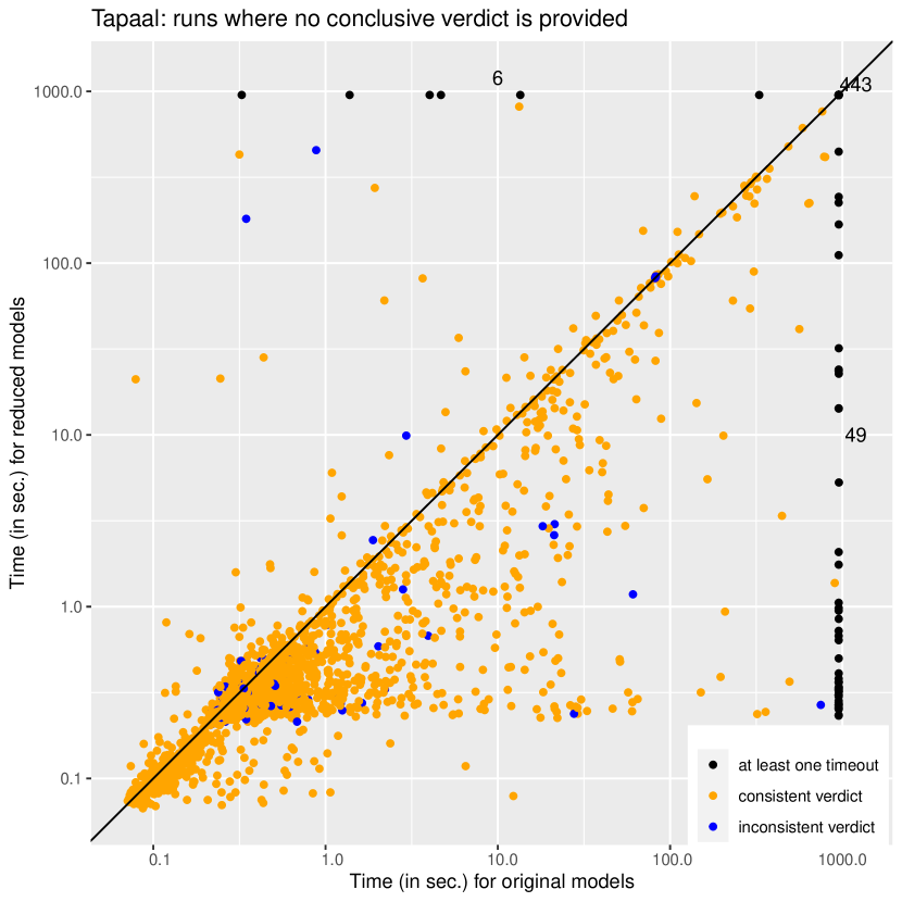
(d) Tapaal on non decidable instances

Figure 4. Experiments on the MCC’2021 LTL benchmark using the two best tool of the MCC contest: Tapaal and ITS-tools. Figures (a) and (c) contain the cases where the verdict of the semi-decisions procedures is reliable, and distinguish cases where the output is True (empty product) and False (non empty product). (b) and (d) display the cases where the verdict is not reliable and distinguish cases where the output is inconsistent with the ground truth from cases where they agree.

4.2. A Study of Performances

Benchmark Setup. Among the LTL benchmarks presented in Table 1, we opted for the MCC benchmark to evaluate the techniques presented in this paper. This benchmark seems relevant since (1) it contains both academic and industrial models, (2) it has a huge set of (random) formulae and (3) includes models so that we could measure the effect of the approach in a model-checking setting. The model-checking competition (MCC) is an annual event in its $10^{th}$ edition in 2021 where competing tools are evaluated on a large benchmark. We use the formulae and models from the latest $2021$ edition of the contest, where Tapaal [DJJ⁺12] was awarded the gold medal and ITS-Tools  [Thi15] was silver in the LTL category of the contest. We evaluate both of these tools in the following performance measures, showing that our strategy is agnostic to the back-end analysis engine. Our experimental setup consists in two steps.

1. Parse the model and formula pair, and analyze the sensitivity of the formula. When the formula is shortening or lengthening insensitive (but not both) output two model/formula pairs: reduced and original. The "original" version does also benefit from reduction rules, but we apply only rules that are compatible with full LTL. The "reduced" version additionally benefits from rules that are reductions at the language level, i.e. mainly pre and post agglomeration (but enacting these rules can cause further simplifications). The original and reduced model/formula pairs that result from this procedure are then exported in the same format the contest uses. This step was implemented within ITS-tools.

2. Run an MCC compatible tool on both the reduced and original versions of each model/formula pair and record the time performance and the verdict.

For the first step, using Spot [MD15], we detect that a formula is either shortening or lengthening insensitive for 99.81% of formulae in less than 1 second. After this analysis, we obtain 12 227 model/formula pairs where the formula is either shortening insensitive or lengthening insensitive (but not both). Among these pairs, in $3005$ cases (24.6%) the model was resistant to the structural reduction rules we use. Since our strategy does not improve such cases, we retain the remaining 9 222 (75.4%) model/formula pairs in the performance plots of Figure 4. We measured that on average 34.19% of places and 32.69% of the transitions of the models were discarded by reduction rules with respect to the "original" model, though the spread is high as there are models that are almost fully reducible and some that are barely so. Application of reduction rules is in complexity related to the size of the structure of the net and takes less than 20 seconds to compute in 95.5% of the models. We are able to treat $9222$ examples (21% of the original $43989$ model/formula pairs of the MCC) using reductions. All these formulae until now could not be handled using reduction techniques.

For the second step, we measured the solution time for both reduced and original model/formula pairs using the two best tools of the MCC’2021 contest. A full tool using our strategy might optimistically first run on the reduced model/formula pair hoping for a definitive answer, but we recommend the use of a portfolio approach where the first reliable answer is kept. In these experiments we neutrally measured the time for taking a semi-decision on the reduced model vs. the time for taking a (complete) decision on the original model. We then classify the results into two sets, decidable instances are shown on the left of Fig. 4 and instances that are not decidable (by our procedure) are on the right. On "decidable instances" our semi-decision procedure could have concluded reliably because the formula is true and the property shortening insensitive or the formula is false and the property lengthening insensitive. Non decidable instances shown on the right are those where the verdict on the reduced model is not to be trusted (or both the original and reduced procedures timed out).

With this workflow we show that our approach is generic and can be easily implemented on top of any MCC compatible model-checking tool. All experiments were run with a 950 seconds timeout (close to 15 minutes, which is generous when the contest offers 1 hour for 16 properties). We used a heterogeneous cluster of machines with four cores allocated to each experiment, and ensured that experiments concerning reduced and original versions of a given model/formula are comparable.

Figure 4 presents the results of these experiments. The results are all presented as log-log scatter plots opposing a run on the original to a run on the reduced model/formula pair. Each dot represents an experiment on a model/formula pair; a dot below the diagonal indicates that the reduced version was faster to solve, while a point above it indicates a case where the reduced model actually took longer to solve than the original (fortunately there are relatively few). Points that timeout for one (or both) of the approaches are plotted on the line at 950 seconds, we also indicate the number of points that are in this line (or corner) next to it.

The plots on the left (a) and (c) correspond to "decidable instances" while those on the right are not decidable by our procedure. The two plots on the top correspond to the performance of ITS-tools, while those on the bottom give the results with Tapaal. The general form of the results with both tools is quite similar confirming that our strategy is indeed responsible for the measured gains in performance and that they are reproducible. Reduced problems are generally easier to solve than the original. This gain is in the best case exponential as is visible through the existence of spread of points reaching out horizontally in this log-log space (particularly on the Tapaal plots).

The colors on the decidable instances reflect whether the verdict was true or false. For false properties a counter-example was found by both procedures interrupting the search, and while the search space of a reduced model is a priori smaller, heuristics and even luck can play a role in finding a counter-example early. True answers on the other hand generally require a full exploration of the state space so that the reductions should play a major role in reducing the complexity of model-checking. The existence of True answers where the reduction fails is surprising at first, but a smaller Kripke structure does not necessarily induce a smaller product as happens sometimes in this large benchmark (and in other reduction techniques such as stubborn sets [Val90]). On the other hand the points aligned to the right of the plots a) and c) (189 for ITS-tools and 119 for Tapaal) correspond to cases where our procedure improved these state of the art tools, allowing to reach a conclusion when the original method fails.

The plots on the right use orange to denote cases where the verdict on the reduced and original models were the same; on these points the procedures had comparable behaviors (either exploring a whole state space or exhibiting a counter-example). The blue color denotes points where the two procedures disagree, with several blue points above the diagonal reflecting cases where the reduced procedure explored the whole state space and thought the property was true while the original procedure found a counter-example (this is the worst case). Surprisingly, even though on these non decidable plots b) and d) our procedure should not be trusted, it mostly agrees (in 95% of the cases) with the decision reached on the original.

Out of the 9222 experiments in total, for ITS-tools 5901 runs reached a trusted decision (64 %), 2927 instances reached an untrusted verdict (32 %), and the reduced procedure timed out in 394 instances (4 %). Tapaal reached a trusted decision in 5866 instances (64 %), 2884 instances reached an untrusted verdict (31 %), and the reduced procedure timed out in 472 instances (5 %). On this benchmark of formulae we thus reached a trusted decision in almost two thirds of the cases using the reduced procedure.

5. Extensions and Perspectives

In this section we investigate how to improve the results obtained in the previous sections, thus extending the presentation of [PPRT22]. The main extension considered is to focus on fragments of a language that satisfy shortening/lengthening/stutter insensitivity criterion, even when the language as a whole is length sensitive. We first introduce tools to partition a property language into these fragments and present experimental evaluation on a benchmark of LTL formulae. We then present possible approaches to confirm non trustworthy answers of the current semi decision procedure, one of which turns out to be applicable to a much wider range of properties. All of this section is new content with respect to [PPRT22].

5.1. Partition of a Language

The idea is to partition the language of the (negation of the) property into four parts: the stutter insensitive part, the pure shortening insensitive part, the pure lengthening insensitive part, and the pure fully length sensitive part. This is a partition of the language, hence the "pure" qualifier indicates that there is no overlap, e.g. the pure shortening insensitive part does not contain any word of the stutter insensitive part of the original language.

Given this partition, we can use the most efficient available procedure to check emptiness of the product of the system with each part. For the first three parts in particular, we can work with a reduction of the system. The stutter insensitive part benefits from a full decision procedure when working working with the reduction, and the partly length insensitive parts can use the semi-decision procedure of Theorem 1.

Length-sensitive partition of a language.

Given a language $\mathscr{L}$, we define:

• The stutter insensitive part of $\mathscr{L}$ noted $SI^{\pm}(\mathscr{L})$ is defined as the largest subset of $\mathscr{L}$ that is stutter insensitive. More precisely $\forall r\in\mathscr{L}$,

  $$r\in SI^{\pm}(\mathscr{L})\Leftrightarrow(\forall r^{\prime}\in\Sigma^{\omega},r^{\prime}{\rm Phys.~{}Rev.~{}E}r\lor r{\rm Phys.~{}Rev.~{}E}r^{\prime}\Rightarrow r^{\prime}\in\mathscr{L})$$

• The pure shortening insensitive part of $\mathscr{L}$ noted $SI^{-}(\mathscr{L})$ is the largest subset of $\mathscr{L}$ that is shortening insensitive but does not intersect with $SI^{\pm}(\mathscr{L})$. More precisely $\forall r\in\mathscr{L}$

  $$r\in SI^{-}(\mathscr{L})\Leftrightarrow\left\{\begin{array}[]{l}\forall r^{\prime}\in\Sigma^{\omega},r^{\prime}{\rm Phys.~{}Rev.~{}E}r\Rightarrow r^{\prime}\in\mathscr{L}\\ \exists r^{\prime\prime}\in\Sigma^{\omega}\setminus\mathscr{L},r{\rm Phys.~{}Rev.~{}E}r^{\prime\prime}\end{array}\right.$$

• The pure lengthening insensitive part of $\mathscr{L}$ noted $SI^{+}(\mathscr{L})$ is the largest subset of $\mathscr{L}$ that is lengthening insensitive but does not intersect with $SI^{\pm}(\mathscr{L})$. More precisely $\forall r\in\mathscr{L}$

  $$r\in SI^{+}(\mathscr{L})\Leftrightarrow\left\{\begin{array}[]{l}\forall r^{\prime}\in\Sigma^{\omega},r{\rm Phys.~{}Rev.~{}E}r^{\prime}\Rightarrow r^{\prime}\in\mathscr{L}\\ \exists r^{\prime\prime}\in\Sigma^{\omega}\setminus\mathscr{L},r^{\prime\prime}{\rm Phys.~{}Rev.~{}E}r\end{array}\right.$$

• The pure fully length sensitive part of $\mathscr{L}$ noted $SS(\mathscr{L})$ is the largest subset of $\mathscr{L}$ that is shortening and lengthening sensitive but does not intersect with the previous parts. More precisely $\forall r\in\mathscr{L}$

  $$r\in SS(\mathscr{L})\Leftrightarrow\left\{\begin{array}[]{l}\exists r^{\prime}\in\Sigma^{\omega}\setminus\mathscr{L},r{\rm Phys.~{}Rev.~{}E}r^{\prime}\\ \exists r^{\prime\prime}\in\Sigma^{\omega}\setminus\mathscr{L},r^{\prime\prime}{\rm Phys.~{}Rev.~{}E}r\end{array}\right.$$

To compute this partition when the language $\mathscr{L}$ is represented by a Buchi automaton $A$, we can reuse the closure ($cl$) and self-loopization ($sl$) syntactic transformations of an automaton introduced in Section 3.3.

Computing the length-sensitive partition of a language.

Let $A$ designate a Büchi automaton recognizing language $\mathscr{L}$.

• Let $B=sl(cl(A))$, let $C=B\otimes\bar{A}$, let $D=sl(cl(C))$, then $SI^{\pm}(A)=A\otimes\overline{D}$

• Let $A^{\prime}=A\otimes\overline{SI(A)}$,

  • Let $B^{-}=cl(A^{\prime})$, let $C^{-}=B^{-}\otimes\overline{A^{\prime}}$, let $D^{-}=sl(C^{-})$, then $SI^{-}(A)=A^{\prime}\otimes\overline{D^{-}}$.

  • Let $B^{+}=sl(A^{\prime})$, let $C^{+}=B^{+}\otimes\overline{A^{\prime}}$, let $D^{+}=cl(C^{+})$, then $SI^{+}(A)=A^{\prime}\otimes\overline{D^{+}}$.

• Finally, $SS(A)=A\otimes\overline{SI(A)}\otimes\overline{SI^{-}(A)}\otimes\overline{SI^{+}(A)}$

The automaton produced in each case matches Definition 5.1, e.g. $\mathscr{L}(SI^{\pm}(A))=SI^{\pm}(\mathscr{L})$ when $A$ recognizes language $\mathscr{L}$. The reasoning behind these definitions is illustrated in Figure 5. For each equivalence class, we simply reason on three distinct but comparable words $r,r^{\prime}$ and $r^{\prime\prime}$ such that $r{\rm Phys.~{}Rev.~{}E}r^{\prime}{\rm Phys.~{}Rev.~{}E}r^{\prime\prime}$. The question for each of these words is whether they belong to the language of $A$ or not. This gives us $2^{3}=8$ cases to consider, but some cases are redundant, e.g. the case where $r$ and $r^{\prime}$ belong to $A$ but $r^{\prime\prime}$ doesn’t is homogeneous to the case where $r$ belongs to $A$ but neither $r^{\prime}$ nor $r^{\prime\prime}$ do. Figure 5 thus only represents the $6$ significantly different cases for a given equivalence class of runs.

[width=]fig/SIpart

(a) Computing the stutter insensitive part $SI^{\pm}$ of the language of an automaton $A$.

[width=]fig/ShortPart

(b) Computing the pure shortening insensitive part $SI^{-}$ of the language of $A$.

Figure 5. Similarly to Fig. 2, $\Sigma^{\omega}$ is represented as a circle that is partitioned into equivalence classes of word (represented as pie slices), and longer words are assumed to be further from the center of the circle. Gray areas are inside the language of the automaton, white are outside of it. In this example six equivalence classes are chosen to cover all different possible situations within an equivalence class.

It can be noted that it is quite easy to adapt the steps to compute less strict versions of these "partitions", e.g. extracting the sublanguage $SI^{\pm}\cup SI^{-}$ can be done using equations for computing $SI^{-}$ (see Fig. 5) but substituting $A$ for $A^{\prime}$ in all equations. This involves less complement operations on automata.

Computing the complement of an automaton $A$ is worst case exponential in the size of $A$ unfortunately, and the procedure described here uses several complement to implement set difference: $\mathscr{L}(A)\setminus\mathscr{L}(B)=\mathscr{L}(A\otimes\bar{B})$. At least when the automaton $A_{\varphi}$ comes from an LTL property, we can compute $A_{\lnot\varphi}$ instead of computing the complement $\bar{A_{\varphi}}$. The other complement operations in our procedure seem unavoidable at this stage however. Despite this high worst case complexity, the complexity of model-checking as a whole is usually dominated by the size of Kripke structure which can be non-trivially reduced by structural reductions. Hence a model-checking procedure using the partition and structural reductions where possible could still be competitive with the default procedure that cannot use structural reductions at all unless the property is fully stutter insensitive.

5.2. Experiments with Partitioning

As preliminary experimentation we computed these partitions on the LTL formulae of Section 4.1 . Results are presented in Table 2.

Bench.	Total	TO+MO	SI	LI	w/ $SI^{\pm}$	ShI	w/ $SI^{\pm}$	LS	w/ $SI^{\pm}$	w/ $SI^{+}$	w/ $SI^{-}$	w/ $SS$
Dwyer	55	0	32	13	13	9	9	1	1	1	1	0
Spot	93	1+0	63	17	17	11	11	2	2	2	2	1
RERS	2050	0	714	777	777	559	559	0	0	0	0	0
MCC	44252	328+40	26146	4996	4994	6161	6146	6581	6527	6498	6573	2799

Table 2. Study of partitioning of properties of the literature. The $SI$ stutter insensitive, $LI$ lengthening insensitive, $ShI$ shortening insensitive and $LS$ length sensitive columns are the same as in Table 1. For $LI$ and $ShI$ we also report the number of cases where the language contains a pure stuttering insensitive part $SI^{\pm}$ (columns $w/SI^{\pm}$), and for the length sensitive properties $LS$ we also report the number of cases in which the $SI^{\pm},SI^{+},SI^{-}$ and $SS$ parts are non empty. TO indicates a timeout of over 15 seconds, and MO indicates a memory overflow when computing the partition.

This table shows that:

• An overwhelming majority (over $99.8\%$ in all cases, and $100\%$ of non random formulae) of shortening or lengthening insensitive properties contain a stutter insensitive sublanguage (column $w/SI^{\pm}$). This perhaps explain the high consistency of results on non decidable instances of Fig 4. This observation is also true of fully length sensitive properties $LS$, with over $99.1\%$ of these properties containing a stutter insensitive sublanguage. At least for this part of the language, strategies using structural reductions and/or partial order reduction are possible.

• While computing the partition of a language can theoretically be prohibitively expensive, in practice in most cases it is possible to do so. We fail to compute the partition for only one property of $Spot$ benchmark, and less than one percent of the MCC full dataset. These measures use a timeout of 15 seconds, which we consider negligible in most cases in the full model-checking procedure that has timeout of the order of several minutes.

• Most length sensitive languages (classified as "LS") are actually a combination of a lengthening insensitive and a shortening insensitive part, typically with some stuttering insensitive behavior added on top (in over $99\%$ of cases), but do not actually contain an $SS$ pure fully length sensitive part. Only $42\%$ of the length sensitive properties of the MCC actually contain a fully sensitive $SS$ part, which only represents $\approx 6\%$ of all model/formula pairs in the MCC (that ITS-Tools could parse). These percentages fall to practically zero on non random formulae.

Overall the results in this table are very encouraging. Studying fragments of the language using the most efficient strategy for each part seems to be a promising approach, particularly for the $LS$ properties for which we would currently default to a study on the non reduced version of the model.

5.3. Extending the language

This section is independent of the two previous sections, and presents a new complementary approach that can help to validate cases where there are no counter-examples.

For any language $\mathscr{L}$, by extension of the closure operation on automaton, let $cl(\mathscr{L})=\{r^{\prime}\in\Sigma^{\omega}\mid\exists r\in\mathscr{L},r^{\prime}{\rm Phys.~{}Rev.~{}E}r\}$.

Given two languages $\mathscr{L}_{\lnot\varphi}$ and $\mathscr{L}_{\mathit{KS}}$, and a reduction function $I$ for $\mathscr{L}_{\mathit{KS}}$ such that $\mathit{Red}_{I}(\mathscr{L}_{\mathit{KS}})$ is a reduction of $\mathscr{L}_{\mathit{KS}}$,

$$cl(\mathscr{L}_{\lnot\varphi})\cap\mathit{Red}_{I}(\mathscr{L}_{\mathit{KS}})=\emptyset\Rightarrow\mathscr{L}_{\lnot\varphi}\cap\mathscr{L}_{\mathit{KS}}=\emptyset$$

Proof 5.1.

Because $cl(\mathscr{L}_{\lnot\varphi})\cap\mathit{Red}_{I}(\mathscr{L}_{\mathit{KS}})=\emptyset$, we are guaranteed in any stutter equivalent class $\hat{r}$ that all words of the reduced language $\mathit{Red}_{I}(\mathscr{L}_{\mathit{KS}})$ in this class (if any exist) are strictly longer than any word in $cl(\mathscr{L}_{\lnot\varphi})$ hence they are strictly longer than any word in $\mathscr{L}_{\lnot\varphi}$. Since $\mathit{Red}_{I}(\mathscr{L}_{\mathit{KS}})$ only contains words that are shorter or equal to words of the original language, $\mathscr{L}_{\mathit{KS}}$ also must contain only words that are strictly longer than any word in $\mathscr{L}_{\lnot\varphi}$.

This observation gives us a new semi-decision procedure (only able to prove absence of counter-examples) that uses a structurally reduced model and can be applied to arbitrary properties. Of course, it is only really relevant for lengthening insensitive or length sensitive properties as stutter insensitive properties enjoy a full decision procedure and shortening insensitive properties are not modified by the $cl$ operation (by definition). Note that for these shortening insensitive properties, we already had established in Theorem 1 that when the product ($\mathscr{L}_{\lnot\varphi}\cap\mathit{Red}_{I}(\mathscr{L}_{\mathit{KS}})$) is empty, the result is reliable.

5.4. Revisiting the decision procedure

A revisited model-checking approach exploiting the new features introduced in this section, and applicable to arbitrary properties could be:

1. First, optimistically compute the product of the property and the reduced $\mathit{KS}$.

2. If the property language is SI, LI or ShI and the verdict is reliable, conclude.

3. Otherwise, try to confirm the verdict obtained:

   • If the product is empty, try to confirm using the product of $cl(A_{\lnot\varphi})$ and the reduced $\mathit{KS}{}$. If this product is empty, conclude.

   • If the product is not empty, try to confirm the existence of a reliable counter-example in the product of $SI^{\pm}\cup SI^{+}$ with the reduced $\mathit{KS}$. If it exists conclude.

4. If these tests fail, we can still try to compute the result for the $SI^{\pm}$ part of the language on the reduced system (since this is a full and reliable decision procedure) and proceed (if the product is empty, otherwise we have a trusted counter-example) to verify the remaining parts of the language on the original $\mathit{KS}$.

Overall for length sensitive properties, separate analysis of the parts of the language $SI^{\pm},SI^{+},SI^{-}$ on the reduced $\mathit{KS}$ (using the most appropriate decision procedure) remains possible, thus extending the scope of properties where at least part of the analysis can be performed using structural reductions.

While the outlined approach has not yet been implemented, the experiments on partitioning of Table 2 indicate that there is a lot of room for these strategies to work (over $99\%$ of properties in the benchmark contain an $SI^{\pm}$ part). Moreover the high correlation ($95\%$) between untrusted verdicts of the semi-decision procedure (see Fig. 4 B) and D)) and actual verdicts seems to indicate that an approach seeking to confirm untrusted verdicts could be very successful.

6. Related Work

Partial order vs structural reductions. Partial order reduction (POR) [PPH96, Val90, Pel94, GW94] is a very popular approach to combat state explosion for stutter insensitive formulae. These approaches use diverse strategies (stubborn sets, ample sets, sleep sets…) to consider only a subset of events at each step of the model-checking while still ensuring that at least one representative of each stutter equivalent class of runs is explored. Because the preservation criterion is based on equivalence classes of runs, this family of approaches is limited only to the stutter insensitive fragment of LTL (see Fig.2). However the structural reduction rules used in this paper are compatible and can be stacked with POR when the formula is stutter insensitive; this is the setting in which most structural reduction rules were originally defined. Hence in the approach where we study either fully $SI$ formulas or simply the $SI^{\pm}$ fragment of the language of the property separately, POR can be stacked on top of our approach for studying this fragment.

Structural reductions in the literature. The structural reductions rules we used in the performance evaluation are defined on Petri nets where the literature on the subject is rich [Ber85, PP00, EHP05, HP06, BLBDZ19, Thi20]. However there are other formalism where similar reduction rules have been defined such as [PPR08] using "atomic" blocks in Promela, transaction reductions for the widely encompassing intermediate language PINS of LTSmin [Laa18], and even in the context of multi-threaded programs [FQ03]. All these approaches are structural or syntactic, they are run prior to model-checking per se.

Non structural reductions in the literature. Other strategies have been proposed that instead of structurally reducing the system, dynamically build an abstraction of the Kripke structure where less observable stuttering occurs. These strategies build a $\mathit{KS}{}$ whose language is a reduction of the language of the original $\mathit{KS}{}$ (in the sense of Def. 2.4), that can then be presented to the emptiness check algorithm with the negation of the formula. They are thus also compatible with the approach proposed in this paper. Such strategies include the Covering Step Graph (CSG) construction of [VM97] where a "step" is performed (instead of firing a single event) that includes several independent transitions. The Symbolic Observation Graph of [KP08] is another example where states of the original $\mathit{KS}{}$ are computed (using BDDs) and aggregated as long as the atomic proposition values do not evolve; in practice it exhibits to the emptiness check only shortest runs in each equivalence class hence it is a reduction.

7. Conclusion

To combat the state space explosion problem that LTL model-checking meets, structural reductions have been proposed that syntactically compact the model so that it exhibits less interleaving of non observable actions. Prior to this work, all of these approaches were limited to the stutter insensitive fragment of the logic. We bring a semi-decision procedure that widens the applicability of these strategies to formulae which are shortening insensitive or lengthening insensitive. The experimental evidence presented shows that the fragment of the logic covered by these new categories is quite useful in practice. An extensive measure using the models, formulae and the two best tools of the model-checking competition 2021 shows that our strategy can improve the decision power of state of the art tools, and confirm that in the best case an exponential speedup of the decision procedure can be attained. We further proposed in this paper approaches that seek to confirm untrusted semi-decision verdicts using a partition of the language, and an approach based on extending the (arbitrary) property language to obtain a procedure that could reliably conclude that the product is empty while working with a reduced system. We also identified several other strategies that are compatible with our approach since they construct a reduced language.

Further work involves implementation and experimentation of the approaches introduced in Section 5, as well as developing approaches based on studying the precise (untrusted) counter-example if one is produced to progressively refine the analysis in a CEGAR manner.

References

- [Ber85] Gérard Berthelot. Checking properties of nets using transformation. In Applications and Theory in Petri Nets, volume 222 of LNCS, pages 19–40. Springer, 1985.
- [BLBDZ19] Bernard Berthomieu, Didier Le Botlan, and Silvano Dal Zilio. Counting Petri net markings from reduction equations. International Journal on Software Tools for Technology Transfer, April 2019.
- [Cou99] Jean-Michel Couvreur. On-the-fly verification of linear temporal logic. In World Congress on Formal Methods, volume 1708 of Lecture Notes in Computer Science, pages 253–271. Springer, 1999.
- [DAC98] Matthew B. Dwyer, George S. Avrunin, and James C. Corbett. Property specification patterns for finite-state verification. In Mark Ardis, editor, Proceedings of the 2nd Workshop on Formal Methods in Software Practice (FMSP’98), pages 7–15. ACM Press, March 1998. doi:10.1145/298595.298598.
- [DJJ+12] Alexandre David, Lasse Jacobsen, Morten Jacobsen, Kenneth Yrke Jørgensen, Mikael H. Møller, and Jiří Srba. TAPAAL 2.0: Integrated development environment for timed-arc Petri nets. In Cormac Flanagan and Barbara König, editors, Tools and Algorithms for the Construction and Analysis of Systems, pages 492–497, Berlin, Heidelberg, 2012. Springer Berlin Heidelberg.
- [EH00] Kousha Etessami and Gerard J. Holzmann. Optimizing Büchi automata. In C. Palamidessi, editor, Proceedings of the 11th International Conference on Concurrency Theory (Concur’00), volume 1877 of LNCS, pages 153–167, Pennsylvania, USA, 2000. Springer-Verlag.
- [EHP05] Sami Evangelista, Serge Haddad, and Jean-François Pradat-Peyre. Syntactical colored Petri nets reductions. In ATVA, volume 3707 of LNCS, pages 202–216. Springer, 2005.
- [FQ03] Cormac Flanagan and Shaz Qadeer. A type and effect system for atomicity. In PLDI, pages 338–349. ACM, 2003.
- [GW94] Patrice Godefroid and Pierre Wolper. A partial approach to model checking. Inf. Comput., 110(2):305–326, 1994.
- [HJM+21] Falk Howar, Marc Jasper, Malte Mues, David Schmidt, and Bernhard Steffen. The rers challenge: towards controllable and scalable benchmark synthesis. International Journal on Software Tools for Technology Transfer, pages 1–14, 06 2021. doi:10.1007/s10009-021-00617-z.
- [HP06] Serge Haddad and Jean-François Pradat-Peyre. New efficient Petri nets reductions for parallel programs verification. Parallel Processing Letters, 16(1):101–116, 2006.
- [KBG+21] F. Kordon, P. Bouvier, H. Garavel, L. M. Hillah, F. Hulin-Hubard, N. Amat., E. Amparore, B. Berthomieu, S. Biswal, D. Donatelli, F. Galla, , S. Dal Zilio, P. G. Jensen, C. He, D. Le Botlan, S. Li, , J. Srba, Y. Thierry-Mieg, A. Walner, and K. Wolf. Complete Results for the 2021 Edition of the Model Checking Contest. http://mcc.lip6.fr/2021/results.php, June 2021.
- [KP08] Kais Klai and Denis Poitrenaud. MC-SOG: an LTL model checker based on symbolic observation graphs. In Kees M. van Hee and Rüdiger Valk, editors, Applications and Theory of Petri Nets, 29th International Conference, PETRI NETS 2008, Xi’an, China, June 23-27, 2008. Proceedings, volume 5062 of LNCS, pages 288–306. Springer, 2008.
- [Laa18] Alfons Laarman. Stubborn transaction reduction. In NFM, volume 10811 of LNCS, pages 280–298. Springer, 2018.
- [Lam90] Leslie Lamport. A theorem on atomicity in distributed algorithms. Distributed Comput., 4:59–68, 1990.
- [Lip75] Richard J. Lipton. Reduction: A method of proving properties of parallel programs. Commun. ACM, 18(12):717–721, 1975.
- [LS89] Leslie Lamport and Fred B. Schneider. Pretending atomicity. SRC Research Report 44, May 1989. URL: https://www.microsoft.com/en-us/research/publication/pretending-atomicity/.
- [MD15] Thibaud Michaud and Alexandre Duret-Lutz. Practical stutter-invariance checks for -regular languages. In SPIN, volume 9232 of LNCS, pages 84–101. Springer, 2015.
- [Pel94] Doron A. Peled. Combining partial order reductions with on-the-fly model-checking. In CAV, volume 818 of LNCS, pages 377–390. Springer, 1994.
- [PP00] Denis Poitrenaud and Jean-François Pradat-Peyre. Pre- and post-agglomerations for LTL model checking. In ICATPN, volume 1825 of LNCS, pages 387–408. Springer, 2000.
- [PPH96] Doron A. Peled, Vaughan R. Pratt, and Gerard J. Holzmann, editors. Partial Order Methods in Verification, Proceedings of a DIMACS Workshop, 1996, volume 29 of DIMACS Series in Discrete Mathematics and Theoretical Computer Science. DIMACS/AMS, 1996.
- [PPR08] Christophe Pajault, Jean-François Pradat-Peyre, and Pierre Rousseau. Adapting Petri nets reductions to Promela specifications. In FORTE, volume 5048 of LNCS, pages 84–98. Springer, 2008.
- [PPRT22] Emmanuel Paviot-Adet, Denis Poitrenaud, Etienne Renault, and Yann Thierry-Mieg. LTL under reductions with weaker conditions than stutter invariance. In FORTE, volume 13273 of Lecture Notes in Computer Science, pages 170–187. Springer, 2022.
- [SB00] Fabio Somenzi and Roderick Bloem. Efficient Büchi automata for LTL formulæ. In Proceedings of the 12th International Conference on Computer Aided Verification (CAV’00), volume 1855 of LNCS, pages 247–263, Chicago, Illinois, USA, 2000. Springer-Verlag.
- [Thi15] Yann Thierry-Mieg. Symbolic model-checking using ITS-tools. In TACAS, volume 9035 of LNCS, pages 231–237. Springer, 2015.
- [Thi20] Yann Thierry-Mieg. Structural reductions revisited. In Petri Nets, volume 12152 of LNCS, pages 303–323. Springer, 2020.
- [Val90] Antti Valmari. A stubborn attack on state explosion. In CAV, volume 531 of LNCS, pages 156–165. Springer, 1990.
- [Var07] Moshe Y. Vardi. Automata-theoretic model checking revisited. In VMCAI, volume 4349 of LNCS, pages 137–150. Springer, 2007.
- [VM97] François Vernadat and François Michel. Covering step graph preserving failure semantics. In Pierre Azéma and Gianfranco Balbo, editors, Application and Theory of Petri Nets 1997, 18th International Conference, ICATPN ’97, Toulouse, France, June 23-27, 1997, Proceedings, volume 1248 of LNCS, pages 253–270. Springer, 1997.