Mind the Gap: Measuring Generalization Performance Across Multiple Objectives

Abstract

Modern machine learning models are often constructed taking into account multiple objectives, e.g., minimizing inference time while also maximizing accuracy. Multi-objective hyperparameter optimization (MHPO) algorithms return such candidate models, and the approximation of the Pareto front is used to assess their performance. In practice, we also want to measure generalization when moving from the validation to the test set. However, some of the models might no longer be Pareto-optimal which makes it unclear how to quantify the performance of the MHPO method when evaluated on the test set. To resolve this, we provide a novel evaluation protocol that allows measuring the generalization performance of MHPO methods and studying its capabilities for comparing two optimization experiments.

1 Introduction

Multi-objective hyperparameter optimization (MHPO; Feurer and Hutter, 2019; Morales-Hernández et al., 2021; Karl et al., 2022) and multi-objective neural architecture search (MNAS; Elsken et al., 2019b; Benmeziane et al., 2021) are becoming increasingly important and enable moving beyond the purely performance-driven selection of machine learning (ML) models. Important additional objectives are, for example, model size, inference time and the number of operations (Elsken et al., 2019a), interpretability (Molnar et al., 2020), feature sparseness (Binder et al., 2020), or fairness (Chakraborty et al., 2019; Cruz et al., 2021; Schmucker et al., 2021). To evaluate and compare multi-objective methods, papers often report the hypervolume indicator of the Pareto front approximation as a measure of optimization performance.

However, as we show in this paper, an ML model that is located on the approximated Pareto front on the validation set can become a dominated model on the test set and vice versa. This phenomenon makes it impossible to compute the hypervolume indicator using the canonical train-validation-test evaluation protocol (Raschka, 2018). To remedy this, we propose a novel evaluation protocol that takes such models into account in order to lay a solid foundation for multi-objective hyperparameter optimization. In addition, we also conduct an initial study in which we use this evaluation protocol to compare the hyperparameter optimization of two machine learning algorithms.

This paper is structured as follows. First, in Section 2, we give background on multi-objective optimization. In Section 3, we then discuss the problem of evaluating generalization performance on a test set and the problems of a naive solution. We go on and describe our new protocol in Section 4 and exemplify it in Section 5. Then, we describe how multi-objective generalization was (not) measured in related work in Section 6 before concluding the paper in Section 7.

We provide Python code to reproduce our experiments at
https://github.com/automl/IDA23-MindTheGap.

2 Background

In the remainder of this paper, we follow the notation from Karl et al. (2022) and aim to minimize the multi-objective function $\bm{c}:\bm{\Lambda}\rightarrow\mathbb{R}^{M}$ defined as $\min_{\bm{\lambda}\in\bm{\Lambda}}\bm{c}(\bm{\lambda})=\min_{\bm{\lambda}\in\bm{\Lambda}}(c_{1}(\bm{\lambda}),\dots,c_{M}(\bm{\lambda}))$, where each $c_{i}:\bm{\Lambda}\rightarrow\mathbb{R}$ denotes the cost of hyperparameter configuration (HPC) $\bm{\lambda}\in\bm{\Lambda}$ according to one cost metric $i\in(1,\dots,M)$. Since, typically, there is no total order on the space of objectives $\mathbb{R}^{M}$, and hence there usually is no single best objective value, we now consider Pareto-dominance and Pareto-optimality instead. Given a function $\bm{c}:\bm{\Lambda}\rightarrow\mathbb{R}^{M}$, we define a binary relation $`\prec`$ on $\mathbb{R}^{M}\times\mathbb{R}^{M}$. Given two cost vectors $\bm{\zeta}^{(1)},\bm{\zeta}^{(2)}\in\mathbb{R}^{M}$, defined as $\bm{\zeta}^{(1)}=\bm{c}(\bm{\lambda}^{(1)})$ and $\bm{\zeta}^{(2)}=\bm{c}(\bm{\lambda}^{(2)})$, we say $\bm{\zeta}^{(1)}$ dominates $\bm{\zeta}^{(2)}$, written as $\bm{\zeta}^{(1)}\prec\bm{\zeta}^{(2)}$, if and only if

$$\forall k\in\left\{1,...,M\right\}:\bm{\zeta}_{k}^{(1)}\leq\bm{\zeta}_{k}^{(2)}\;\land\;\exists l\in\left\{1,...,M\right\}:\bm{\zeta}_{l}^{(1)}<\bm{\zeta}_{l}^{(2)}.$$

We similarly define a dominance relationship for configurations $\bm{\lambda}$: A configuration $\bm{\lambda}^{(1)}$ dominates another configuration $\bm{\lambda}^{(2)}$, so $\bm{\lambda}^{(1)}\prec\bm{\lambda}^{(2)}$. if and only if $\bm{c}(\bm{\lambda}^{(1)})\prec\bm{c}(\bm{\lambda}^{(2)})$. The non-dominated set of solutions, the Pareto front $\mathcal{P}$, is then given by $\mathcal{P}=\{\bm{\zeta}\in\bm{c}(\bm{\Lambda})\,|\,\nexists\,\bm{\zeta}^{\prime}\in\bm{c}(\bm{\Lambda})\text{ s.t. }\bm{\zeta}^{\prime}\prec\bm{\zeta}\}$ and conversely, the Pareto set as the pre-image of $\mathcal{P}$: $\mathcal{P}_{\bm{\Lambda}}=\bm{c}^{-1}(\mathcal{P})=\{\bm{\lambda}\in\bm{\Lambda}\,|\,\nexists\,\bm{\lambda}^{\prime}\in\bm{\Lambda}\text{ s.t. }\bm{\lambda}^{\prime}\prec\bm{\lambda}\}$.

An MHPO algorithm then aims to return the best approximation of the Pareto front, trading off all given objectives. To obtain candidate HPCs $\bm{\lambda}^{(i)}$, an MHPO algorithm iteratively generates and evaluates HPCs $\{\bm{\lambda}^{(1)},\bm{\lambda}^{(2)},\dots,\bm{\lambda}^{(T)}\}$. In the next step, the MHPO algorithm compares the performance of all evaluated solutions to obtain the subset of HPCs $\tilde{P}_{\bm{\Lambda}}\subseteq\{\bm{\lambda}^{(1)},\bm{\lambda}^{(2)},\dots,\bm{\lambda}^{(T)}\}$ approximating the Pareto set and thereby also the Pareto front.

The literature provides several quality metrics for Pareto-optimal sets focusing on different aspects (Zitzler et al., 2000, 2003; Emmerich and Deutz, 2018): (1) Approximation quality of the Pareto front, (2) a good (often uniform) distribution of solutions, and (3) diversity w.r.t. to the values for each metric. Here, we consider the commonly used hypervolume indicator (Karl et al., 2022), i.e., the volume of the objective space covered by the dominating solutions w.r.t. a reference point. The hypervolume indicator mostly considers (1), and it can be used to capture the performance of an MHPO experiment in a single value.

While we discuss our work in the context of MHPO, the background, problem, and proposed solution also apply to other multi-objective optimization problems which involve separate validation and test sets, such as neural architecture search (NAS; Elsken et al., 2019b), Automated Machine Learning (AutoML; Hutter et al., 2019), or ensemble learning.

3 Evaluating Generalization

Having discussed how to evaluate an MHPO method in general, we now turn to the problem that in ML, the predictive performance is usually measured on unseen test data. To highlight the challenges, we summarize the standard evaluation protocol, describe a previously unknown failure mode, hypothesize a naive solution and point out two potential issues of such a naive solution.

In MHPO, we typically tune the hyperparameters of an ML model on a supervised ML task, e.g., classification, with dataset $\mathcal{D}=[(\bm{x},y)^{(1)},\dots,(\bm{x},y)^{(d)}]$. We consider minimizing data-based costs $c_{i}$ that estimate an empirical risk w.r.t. to the entire data distribution, e.g., the empirical risk, fairness metrics, or explainability scores (in contrast to model-based costs, such as inference time or model size). Because we only have access to a finite sample from the entire data distribution, we estimate this risk using the canonical train-validation-test protocol (Raschka, 2018), which trains models on the train portion of the data, and validation & test costs are estimated on the respective data splits (one could also use other protocols, such as cross-validation with a test set). Empirically estimating validation and test costs induces separate estimation errors. Validation set quantities are used for MHPO and to approximate the Pareto front. This approximation is then evaluated on the test set to obtain an unbiased estimate of the generalization error and also to measure the performance of MHPO.

Problems in the Multi-Objective Setting. Due to these separate estimation errors, an HPC deemed Pareto-optimal on the validation set is not necessarily Pareto-optimal on the test set. We visualize this in Figure 1. On the left-hand side, the Pareto front approximation generalizes well to the test set. In the middle, all HPCs are still Pareto-optimal but switch order, which could lead to unexpected performance degradation when selecting an HPC to deploy in practice. However, on the right-hand side, two HPCs are no longer Pareto-optimal, i.e., the Pareto front approximation does not generalize to the test set and contains dominated solutions. We would like to highlight that the two problems depicted in the two right-most plots were so far not discussed in the literature, yet, their existence thwarts the evaluation of MHPO algorithms.

(a)	(b)	(c)

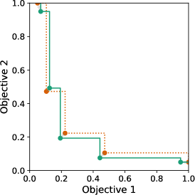
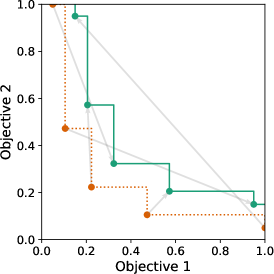
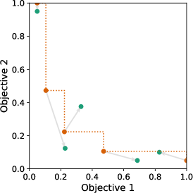
Figure 1: We visualize validation (orange) and test performance (green) of the Pareto set, as found on the validation data set. Considering test performance, (a) all configurations are non-dominated, (b) the configurations are still Pareto-optimal, but switch order, and (c) the configurations are no longer Pareto-optimal.

A naive solution. Discarding dominated solutions based on the test set – which would not be possible in practice because we can only access test labels once in the end to compute final performance – would enable us to compute the hypervolume indicator. For this, we can either consider all evaluated HPCs (as common in assessing the performance of multi-objective methods) or expect the MHPO method to return a reasonable subset (which it believes to be Pareto-optimal). Then, we evaluate these HPCs on the test set, compute the Pareto front approximation based on the test scores, and finally calculate the hypervolume indicator. Unfortunately, this raises the following two issues.

Issue 1: Overestimation. We discard dominated points and thus overestimate the true hypervolume of the returned solutions, i.e., ignore solutions that are no longer part of the Pareto set, as displayed in the left-hand-side plot in Figure 2. In practice, a user could pick one of the discarded solutions (based on its validation performance) and observe a worse performance than what we computed as the generalization performance of the optimization method.

Issue 2: Test data leakage. An adversarial MHPO method could exploit this procedure by returning as many models as possible and thus implicitly selecting its Pareto-optimal set based on the test set, as visualized in the middle of Figure 1. While such a system would seemingly obtain a good score, its benefit in practice is limited.

These two issues emphasize the need for a new evaluation protocol that can detect these issues so that we can develop MHPO methods that return reliable Pareto front approximations.

4 A New Protocol to Measure Generalization

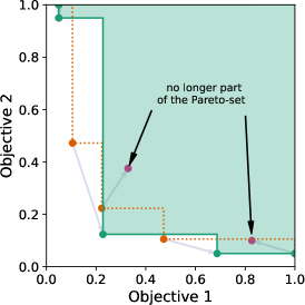
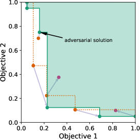
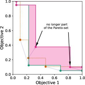
Figure 2: We visualize validation (orange) and test performance (green/pink) of the Pareto set, as found on the validation data set. Left: We show that ignoring dominated points on the test set leads to an overestimation of the hypervolume indicator. Middle: We show how adversarial MHPO can return points that lead to an increased hypervolume on the test data. Right: We show our proposed optimistic Pareto-set (green), pessimistic Pareto-set (pink), and the approximation gap between the optimistic and pessimistic Pareto-set (pink area).

We propose a new evaluation protocol to assess the performance and robustness of an MHPO method reliably. We introduce the concept of optimistic and pessimistic approximations of the Pareto front. We visualize this on the right-hand side of Figure 2. Given an approximation of a Pareto front $\tilde{\mathcal{P}}$ that was computed using the validation split of a data set, we formally define the optimistic Pareto front as

$$\mathcal{P}_{optimistic}=\{\bm{\zeta}\in\bm{c}(\tilde{\mathcal{P}})\,|\,\nexists\;\bm{\zeta}^{\prime}\in\bm{c}(\tilde{\mathcal{P}})\text{ s.t. }\bm{\zeta}^{\prime}\prec_{test}\bm{\zeta}\},$$ (1)

where $\prec_{test}$ denotes a dominance relationship between costs $\bm{\zeta}$ and $\bm{\zeta}^{\prime}$ evaluated on the test set instead of the validation set. Similarly, we define the pessimistic Pareto front as

$$\mathcal{P}_{pessimistic}=\{\bm{\zeta}\in\bm{c}(\tilde{\mathcal{P}})\,|\,\nexists\;\bm{\zeta}^{\prime}\in\bm{c}(\tilde{\mathcal{P}})\text{ s.t. }\bm{\zeta}\prec_{test}\bm{\zeta}^{\prime}\}.$$ (2)

Then, we can compute the hypervolume for both approximations. The difference between both volumes indicates how robust the Pareto front approximation is when going to test data, and we refer to it as the approximation gap. If it is zero, the Pareto set remains identical when moving from validation to test data. If it is greater than zero, then returned HPCs are dominated on the test data.

We can now compare two MHPO methods, A and B, based on their hypervolume using the following three criteria: (1) hypervolume difference: by checking if the optimistic estimate of the hypervolume of an MHPO method A is smaller than the pessimistic estimate of the hypervolume of an MHPO method B, (2) dominance: by using the notion of the optimistic and pessimistic Pareto set to check if pessimistic Pareto front approximation of A dominates the optimistic Pareto front approximation of B, following the popular idea of Pareto front dominance (Emmerich and Deutz, 2018), and (3) approximation gap: by comparing the gap between the optimistic and pessimistic hypervolume across MHPO methods whereas a smaller gap indicates a more robust approximation of the Pareto front.

5 Experimental Evaluation

In this section, we first show that the approximation gap appears in practice and second, experimentally check whether we can now compare algorithms again.

5.1 Demonstration of Approximation Gap

We first demonstrate the existence of the approximation gap by tuning the hyperparameters of a machine learning algorithm. Concretely, we tune the hyperparameters of a random forest model (Breiman, 2001) with $40$ iterations of random search (Bergstra and Bengio, 2012) on the German credit dataset (Dua and Graff, 2017). We provide the configuration space and dataset description in Appendix 0.A. We use precision and recall as objectives, motivated by the fact that both are often ad-hoc combined into the F1 score (Manning et al., 2008) despite this being an inherently multi-objective problem. Following Horn and Bischl (2016), we tune class weights to account for the unbalanced targets. We split the dataset into 60% train, 20% valid, and 20% test data. For every HPC, we train a single model, record the precision and recall metrics on both the validation and test set and visualize the results in Figure 3.

The plots are similarly structured as Figures 1 and 2, and we depict validation performance (in orange) and test performance (in green) w.r.t. both objectives for all evaluated HPCs. The left-hand-side plot highlights the validation losses and the approximation of the Pareto front using the validation set. The middle plot shows how the performance changes when evaluating these HPCs on the test set. Furthermore, we show the hypothetical true Pareto-set $\tilde{\mathcal{P}}_{test}$ on the test data (which we cannot compute in practice; in grey). The right-hand-side plot shows the optimistic (in green) and pessimistic Pareto-set (in pink), which we described above. We observe $\tilde{\mathcal{P}}_{test}\prec\mathcal{P}_{optimistic}\prec\mathcal{P}_{pessimistic}$, while perfect generalization to the test set would give us $\tilde{\mathcal{P}}_{test}=\mathcal{P}_{optimistic}=\mathcal{P}_{pessimistic}$.

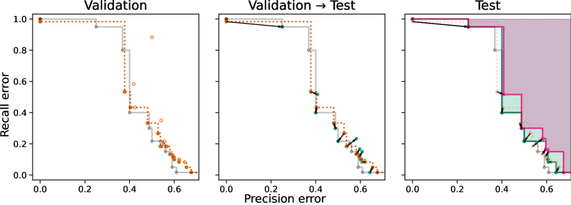
Figure 3: Precision vs Recall. The left plot focuses on the validation error, the middle plot depicts the test error of points from the Pareto set on the validation set, and the right-hand-side plot depicts the approximation of the optimistic and the pessimistic Pareto sets.

5.2 Can We Compare Two Algorithms Again?

Having seen the approximation gap, we now experimentally check whether the three criteria introduced in Section 4 enable comparisons between two different algorithms again. For this, we optimize the hyperparameters of a random forest and a linear classifier with random search for 50, 100, 200, and 500 iterations. We use the same experimental setup and configuration space for the random forest as above and display the configuration space for the linear model in Appendix 0.A.

Table 1: Hypervolume indicators and approximation gap obtained by random search optimizing the hyperparameters of a random forest (top) and a linear model (bottom).

		50	100	200	500
Random Forest	Validation HV	$\ 0.5660$	$\ 0.6357$	$\ 0.6426$	$\ 0.6563$
	Pessimistic HV	$0.5651$	$0.5972$	$0.6060$	$0.5721$
	Optimistic HV	$0.5833$	$0.6128$	$0.6272$	$0.6382$
	Approximation Gap	$0.0181$	$0.0156$	$0.0212$	$0.0661$
Linear Model	Validation HV	$0.5804$	$0.5943$	$0.6330$	$0.6340$
	Pessimistic HV	$0.5970$	$0.5628$	$0.5860$	$0.5641$
	Optimistic HV	$0.5989$	$0.5798$	$0.5994$	$0.5918$
	Approximation Gap	$0.0009$	$0.0170$	$0.0134$	$0.0277$

First, we show the hypervolume indicator on the validation set, the pessimistic and optimistic hypervolume indicator, and the approximation gap in Table 1. As expected, we see that the validation hypervolume increases monotonically with more function evaluations, and after 100 function evaluations, the random forest has a larger validation hypervolume than the linear model, even with 500 function evaluations. Next, we look at the pessimistic and optimistic hypervolume. We can observe that there is no guarantee that they increase together with the validation hypervolume, which means that solutions obtained on the validation set do not generalize to the test set. This can be seen, for example, for the random forest, where the pessimistic hypervolume decreases when going from 200 to 500 function evaluations, while the optimistic hypervolume increases. For the linear model, we can even observe that both the optimistic and pessimistic hypervolume decrease, which can be seen when going from 50 to 100 and from 200 to 500 function evaluations. We can now also compare the two algorithms by comparing the hypervolume indicators (method (1) from Section 4), checking whether the pessimistic hypervolume indicator of one algorithm is larger than the optimistic hypervolume indicator of the other. Using this comparison method, we can conclude (1) that the linear model performs better than the random forest after 50 MHPO function evaluations, (2) that we cannot make a statement about 100 function evaluations, (3) that the random forest is better after 200 function evaluations, and (4) that we cannot make a statement at 500 function evaluations.

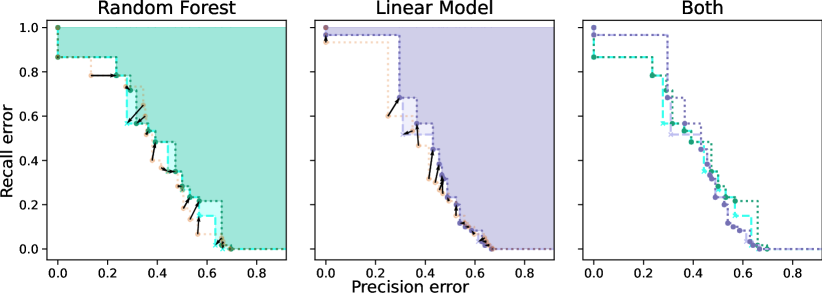
Figure 4: Optimistic and pessimistic Pareto fronts for the random forest (left), the linear model (middle), and both (right) after 200 iterations of random search. For both models, we plot the pessimistic Pareto front in a darker color and using circle markers and the optimistic Pareto front in a lighter color and using star markers; and we use the same colors in the plot on the right-hand side. Furthermore, in the left and middle plots, we also give the validation Pareto front in light orange (similar to Figure 3).

Second, we display the Pareto fronts of the two optimized algorithms in Figure 4 to check whether one Pareto front dominates the other (method (2) from Section 4). We display results after 200 function evaluations, i.e., when the pessimistic hypervolume of the random forest is higher than the optimistic hypervolume of the linear model. This hypervolume dominance is a necessary but not a sufficient condition for Pareto front dominance. In this case, there are indeed solutions for the linear model (denoted as SGD) that are not dominated by the Pareto front of the random forest, making it impossible to state that one model is generally better than the other.

Finally, we examine the approximation gap of the two MHPO algorithms (method (3) from Section 4). The approximation gap is not a monotonic function. It can decrease when the number of function evaluations of the search algorithm increases (random forest from 50 to 100 function evaluations and linear model from 100 to 200 function evaluations). However, the approximation gap can become quite large as we can observe for the random forest with 500 function evaluations, where its size is 10% of the optimistic hypervolume. Also, the approximation gap can be larger than any hypervolume measurement over time, and we argue that this makes it impossible to conclude whether the tuned algorithm actually has improved. On a positive note, we also observe that the two different algorithms appear to have different approximation gaps, which suggests that there are machine learning models that provide more stable solutions.

We conclude this section by answering the question in the section name: yes, the new evaluation protocol allows us to measure the generalization performance of an MHPO algorithm and thereby also to compare two MHPO algorithms or two machine learning models optimized by one MHPO algorithm again.

6 Prior Evaluation Protocols for Multi-Objective Optimization

This section reviews how prior works address the problem of measuring generalization performance in a multi-objective setting. We would first like to note that our setup differs from standard optimization problems under noise since we cannot recover the true function value by repeatedly evaluating the function of interest. However, in our case, the performance of a model selected on the validation set suffers from a distribution shift on the test set. We are unaware of a method for describing such distribution shifts that happen when moving from the validation to the test set.

To the best of our knowledge, no one has yet explicitly studied how to measure the generalization error of HPCs for machine learning models in a multi-objective setting. We found two works that evaluate multi-objective generalization: Horn et al. (2017) use the naive protocol we outline above, and Binder et al. (2020) solely compute, what we call, the optimistic Pareto front. Nonetheless, we would like to emphasize that these works employ these measures in an ad-hoc fashion without any discussion or justification. In contrast, we thoroughly introduce the approximation gap and the concepts behind it. In the field of MHPO, we found that researchers so far use scalarization to choose a final model to evaluate (Cruz et al., 2021), pick a model based on a single metric (Gardner et al., 2019), or use handcrafted heuristics to select a final model (Feffer et al., 2022).

A similar problem exists for constrained optimization: a solution that satisfies the constraints on the validation set can violate the constraint on the test set. Hernández-Lobato et al. (2016) found that "When the constraints are noisy, reporting the best observation is an overly optimistic metric because the best feasible observation might be infeasible in practice" and evaluate a "ground-truth score" by evaluating the final recommendation multiple times, treating a constrained violation as $100\%$ classification error. They tuned a neural network on MNIST under inference time constraints and tuned Hamiltonian Monte Carlo under the constraint that the generated samples pass convergence diagnostic tests. In the field of noisy constrained Bayesian optimization, researchers have suggested an identification step to select the best point after optimization (Gelbart et al., 2014), and Letham et al. (2018) study the proportion of replicates in which the proposed method manages to find suitable solutions, but without scalarizing the final objective as done by Hernández-Lobato et al. (2016).

Moreover, for the problem of multi-objective ranking and selection (identification of the Pareto set from a finite set of choices), the F1 metric was proposed for judging the final result (Gonzalez et al., 2022). However, this does not quantify the solution quality in performance space. Last, the terminology of optimistic and pessimistic Pareto set has also been used in the context of approximating a Pareto front from the predictions of a probabilistic model (Iqbal et al., 2020).

7 Conclusions and Future Work

We have demonstrated that the standard evaluation protocol for single-objective HPO is inapplicable in the multi-objective setting and, as a remedy, introduced optimistic and pessimistic Pareto sets. Based on these, we can compare multi-objective algorithms using the hypervolume difference, dominance, or the new approximation gap. Furthermore, we can detect if the MHPO algorithm leads to an unstable solution, i.e., a large approximation gap, the analogue to over-fitting in single-objective optimization. In an experimental study, we have verified the existence of the approximation gap and demonstrated that we can now compare two machine learning models optimized for multiple metrics again.

In the future, we plan to (1) measure the effect of this problem over a large number of datasets and varying numbers of function evaluations, (2) extend our analysis to take measurement noise into account and (3) extend our protocol to multiple repetitions and cross-validation. Furthermore, we want to (4) evaluate additional multi-objective problems, e.g., trading off true-positive rates and false-positive rates (Levesque et al., 2011; Horn and Bischl, 2016; Karl et al., 2022) or fairness and predictive performance (Chakraborty et al., 2019; Cruz et al., 2021; Schmucker et al., 2021) and (5) study the related problem of distribution shifts in data streams.

Acknowledgements

Robert Bosch GmbH is acknowledged for financial support. Also, this research was partially supported by TAILOR, a project funded by EU Horizon 2020 research and innovation programme under GA No 952215. The authors of this work take full responsibility for its content.

Appendix 0.A Experimental Details

Random Forest		Linear Model
Hyperparameter name	Search space	Hyperparameter name	Search Space
criterion	[gini, entropy]	penalty	[l2, l1, elasticnet]
bootstrap	[True, False]	alpha	$[1e-6,1e-2]$, log
max_features	$[0.0,1.0]$	l1 ratio	$[0.0,1.0]$
min_samples_split	$[2,20]$	fit_intercept	[True, False]
min_samples_leaf	$[1,20]$	eta0	$[1e-7,1e-1]$
pos_class_weight exponent	$[-7,7]$	pos_class_weight exp.	$[-7,7]$

We provide the random forest and linear model search spaces in Table 0.A. We fit the linear model with stochastic gradient descent and use an adaptive learning rate and minimize the log loss (please see the scikit-learn (Pedregosa et al., 2011) documentation for a description of these). Because we are dealing with unbalanced data, we consider the class weights as a hyperparameter and tune the weight of the minority (positive) class in the range of $[2^{-7},2^{7}]$ on a log-scale (Konen et al., 2011; Horn and Bischl, 2016). To deal with categorical features, we use one hot encoding. We transform the features for the linear models using a quantile transformer with a normal output distribution.

We use the German credit dataset (Dua and Graff, 2017) because it is relatively small, leading to high variance in the algorithm performance, and unbalanced. We downloaded the dataset from OpenML (Vanschoren et al., 2014) using the OpenML-Python API (Feurer et al., 2021) as task ID $31$, but conducted our own 60/20/20 split. It is a binary classification problem with 30% positive samples. The dataset has 1000 samples and 20 features. Out of the 20 features, 13 are categorical. The dataset contains no missing values.

References

- Benmeziane et al. (2021) Benmeziane, H., El Maghraoui, K., Ouarnoughi, H., Niar, S., Wistuba, M., Wang, N.: A comprehensive survey on Hardware-aware Neural Architecture Search. arXiv:2101.09336 [cs.LG] (2021)
- Bergstra and Bengio (2012) Bergstra, J., Bengio, Y.: Random search for hyper-parameter optimization. Journal of Machine Learning Research 13, 281–305 (2012)
- Binder et al. (2020) Binder, M., Moosbauer, J., Thomas, J., Bischl, B.: Multi-objective hyperparameter tuning and feature selection using filter ensembles. In: Ceberio, J. (ed.) Proceedings of the Genetic and Evolutionary Computation Conference (GECCO’20), pp. 471––479, ACM Press (2020)
- Breiman (2001) Breiman, L.: Random forests. Machine Learning Journal 45, 5–32 (2001)
- Chakraborty et al. (2019) Chakraborty, J., Xia, T., Fahid, F., Menzies, T.: Software engineering for fairness: A case study with Hyperparameter Optimization. In: Proceedings of the 34th IEEE/ACM International Conference on Automated Software Engineering (ASE), IEEE (2019)
- Cruz et al. (2021) Cruz, A., Saleiro, P., Belem, C., Soares, C., Bizarro, P.: Promoting fairness through hyperparameter optimization. In: Bailey, J., Miettinen, P., Koh, Y., Tao, D., Wu, X. (eds.) Proceedings of the IEEE International Conference on Data Mining (ICDM’21), pp. 1036–1041, IEEE (2021)
- Dua and Graff (2017) Dua, D., Graff, C.: UCI machine learning repository (2017)
- Elsken et al. (2019a) Elsken, T., Metzen, J., Hutter, F.: Efficient multi-objective Neural Architecture Search via lamarckian evolution. In: Proceedings of the International Conference on Learning Representations (ICLR’19) (2019a), published online: iclr.cc
- Elsken et al. (2019b) Elsken, T., Metzen, J., Hutter, F.: Neural Architecture Search: A survey. Journal of Machine Learning Research 20(55), 1–21 (2019b)
- Emmerich and Deutz (2018) Emmerich, M., Deutz, A.: A tutorial on multiobjective optimization: fundamentals and evolutionary methods. Natural Computing 17(3), 585–609 (2018)
- Feffer et al. (2022) Feffer, M., Hirzel, M., Hoffman, S., Kate, K., Ram, P., Shinnar, A.: An empirical study of modular bias mitigators and ensembles. arXiv:2202.00751 [cs.LG] (2022)
- Feurer and Hutter (2019) Feurer, M., Hutter, F.: Hyperparameter Optimization. In: Hutter et al. (2019), chap. 1, pp. 3 – 38, available for free at http://automl.org/book
- Feurer et al. (2021) Feurer, M., van Rijn, J., Kadra, A., Gijsbers, P., Mallik, N., Ravi, S., Müller, A., Vanschoren, J., Hutter, F.: OpenML-Python: an extensible Python API for OpenML. Journal of Machine Learning Research 22(100), 1–5 (2021)
- Gardner et al. (2019) Gardner, S., Golovidov, O., Griffin, J., Koch, P., Thompson, W., Wujek, B., Xu, Y.: Constrained multi-objective optimization for automated machine learning. In: Singh, L., De Veaux, R., Karypis, G., Bonchi, F., Hill, J. (eds.) Proceedings of the International Conference on Data Science and Advanced Analytics (DSAA’19), pp. 364–373, ieeecis, IEEE (2019)
- Gelbart et al. (2014) Gelbart, M., Snoek, J., Adams, R.: Bayesian optimization with unknown constraints. In: Zhang, N., Tian, J. (eds.) Proceedings of the 30th conference on Uncertainty in Artificial Intelligence (UAI’14), pp. 250–258, AUAI Press (2014)
- Gonzalez et al. (2022) Gonzalez, S., Branke, J., van Nieuwenhuyse, I.: Multiobjective ranking and selection using stochastic Kriging. arXiv:2209.03919 [stat.ML] (2022)
- Hernández-Lobato et al. (2016) Hernández-Lobato, J., Gelbart, M., Adams, R., Hoffman, M., Ghahramani, Z.: A general framework for constrained Bayesian optimization using information-based search. Journal of Machine Learning Research 17(1), 5549–5601 (2016)
- Horn and Bischl (2016) Horn, D., Bischl, B.: Multi-objective parameter configuration of machine learning algorithms using model-based optimization. In: Likas, A. (ed.) 2016 IEEE Symposium Series on Computational Intelligence (SSCI), pp. 1–8, IEEE (2016)
- Horn et al. (2017) Horn, D., Dagge, M., Sun, X., Bischl, B.: First investigations on noisy model-based multi-objective optimization. In: Trautmann, H., Rudolph, G., Klamroth, K., Schütze, O., Wiecek, M., Jin, Y., Grimme, C. (eds.) Evolutionary Multi-Criterion Optimization, pp. 298–313, Lecture Notes in Computer Science, Springer (2017)
- Hutter et al. (2019) Hutter, F., Kotthoff, L., Vanschoren, J. (eds.): Automated Machine Learning: Methods, Systems, Challenges. Springer (2019), available for free at http://automl.org/book
- Iqbal et al. (2020) Iqbal, M., Su, J., Kotthoff, L., Jamshidi, P.: Flexibo: Cost-aware multi-objective optimization of deep neural networks. arXiv:2001.06588 [cs.LG] (2020)
- Karl et al. (2022) Karl, F., Pielok, T., Moosbauer, J., Pfisterer, F., Coors, S., Binder, M., Schneider, L., Thomas, J., Richter, J., Lang, M., Garrido-Merchán, E., Branke, J., Bischl, B.: Multi-objective hyperparameter optimization – an overview. arXiv:2206.07438 [cs.LG] (2022)
- Kirschner et al. (2020) Kirschner, J., Bogunovic, I., Jegelka, S., Krause, A.: Distributionally robust Bayesian optimization. In: Chiappa, S., Calandra, R. (eds.) Proceedings of the 23rd International Conference on Artificial Intelligence and Statistics (AISTATS’20), pp. 2174–2184, Proceedings of Machine Learning Research (2020)
- Konen et al. (2011) Konen, W., Koch, P., Flasch, O., Bartz-Beielstein, T., Friese, M., Naujoks, B.: Tuned data mining: a benchmark study on different tuners. In: Krasnogor, N. (ed.) Proceedings of the 13th Annual Conference on Genetic and Evolutionary Computation (GECCO’11), pp. 1995–2002, ACM Press (2011)
- Letham et al. (2018) Letham, B., Brian, K., Ottoni, G., Bakshy, E.: Constrained Bayesian optimization with noisy experiments. Bayesian Analysis (2018)
- Levesque et al. (2011) Levesque, J.C., Durand, A., Gagne, C., Sabourin, R.: Multi-objective evolutionary optimization for generating ensembles of classifiers in the roc space. In: Soule, T. (ed.) Proceedings of the 14th Annual Conference on Genetic and Evolutionary Computation (GECCO’12), p. 879–886, ACM Press (2011)
- Manning et al. (2008) Manning, C., Raghavan, P., Schütze, H.: Introduction to Information Retrieval. Cambridge University Press (2008)
- Molnar et al. (2020) Molnar, C., Casalicchio, G., Bischl, B.: Quantifying model complexity via functional decomposition for better post-hoc interpretability. In: Cellier, P., Driessens, K. (eds.) Machine Learning and Knowledge Discovery in Databases (ECML/PKDD’19), Communications in Computer and Information Science, vol. 1167, pp. 193–204, Springer (2020)
- Morales-Hernández et al. (2021) Morales-Hernández, A., Nieuwenhuyse, I.V., Gonzalez, S.: A survey on multi-objective hyperparameter optimization algorithms for machine learning. arXiv:2111.13755 [cs.LG] (2021)
- Pedregosa et al. (2011) Pedregosa, F., Varoquaux, G., Gramfort, A., Michel, V., Thirion, B., Grisel, O., Blondel, M., Prettenhofer, P., Weiss, R., Dubourg, V., Vanderplas, J., Passos, A., Cournapeau, D., Brucher, M., Perrot, M., Duchesnay, E.: Scikit-learn: Machine learning in Python. Journal of Machine Learning Research 12, 2825–2830 (2011)
- Raschka (2018) Raschka, S.: Model evaluation, model selection, and algorithm selection in machine learning. arXiv:1811.12808 [stat.ML] (2018)
- Schmucker et al. (2021) Schmucker, R., Donini, M., Zafar, M., Salinas, D., Archambeau, C.: Multi-objective asynchronous successive halving. arXiv:2106.12639 [stat.ML] (2021)
- Vanschoren et al. (2014) Vanschoren, J., van Rijn, J., Bischl, B., Torgo, L.: OpenML: Networked science in machine learning. SIGKDD Explorations 15(2), 49–60 (2014)
- Zitzler et al. (2000) Zitzler, E., Deb, K., Thiele, L.: Comparison of multiobjective evolutionary algorithms: Empirical results. Evolutionary computation 8(2), 173–195 (2000)
- Zitzler et al. (2003) Zitzler, E., Thiele, L., Laumanns, M., Fonseca, C., Fonseca, V.: Performance assessment of multiobjective optimizers: An analysis and review. IEEE Transactions on Evolutionary Computation 7, 117–132 (2003)