Photometric and Structural Parameters of Newly Discovered Nuclear Star Clusters in Local Volume Galaxies

Abstract

We use high-resolution Hubble Space Telescope imaging data of dwarf galaxies in the Local Volume ($\lesssim$11\text{\,}\mathrm{Mpc}$$) to parameterise $19$ newly discovered nuclear star clusters (NSCs). Most of the clusters have stellar masses of $M_{\star}^{\mathrm{nsc}}\lesssim${10}^{6}\text{\,}\mathrm{M_{\odot}}$$ and compare to Galactic globular clusters in terms of ellipticity, effective radius, stellar mass, and surface density. The clusters are modelled with a Sérsic profile and their surface brightness evaluated at the effective radius reveals a tight positive correlation to the host galaxy stellar mass. Our data also indicate an increase in slope of the density profiles with increasing mass, perhaps indicating an increasing role for in-situ star formation in more massive hosts. We evaluate the scaling relation between the clusters and their host galaxy stellar mass to find an environmental dependence: for NSCs in field galaxies, the slope of the relation is $\alpha=0.82^{+0.08}_{-0.08}$ whereas $\alpha=0.55^{+0.06}_{-0.05}$ for dwarfs in the core of the Virgo cluster. Restricting the fit for the cluster to $M_{\star}^{\mathrm{gal}}\geq$e6.5\text{\,}\mathrm{M_{\odot}}$$ yields $\alpha=0.70^{+0.08}_{-0.07}$, in agreement with the field environment within the $1\sigma$ interval. The environmental dependence is due to the lowest-mass nucleated galaxies and we speculate that this is either due to an increased number of progenitor globular clusters merging to become an NSC, or due to the formation of more massive globular clusters in dense environments, depending on the initial globular cluster mass function. Our results clearly corroborate recent results in that there exists a tight connection between NSCs and globular clusters in dwarf galaxies.

1 Introduction

The central regions of galaxies are interesting because of the extreme objects they host. Besides supermassive black holes (SMBHs), which are believed to be common in high-mass galaxies (Kormendy & Ho, 2013), nuclear star clusters (NSCs) often occupy the centers of low- to intermediate-mass galaxies. Their size of typically a few parsecs (e.g. Georgiev & Böker, 2014; Carson et al., 2015; Pechetti et al., 2020) and high stellar mass ($M_{\star}^{\mathrm{nsc}}\sim${10}^{7}\text{\,}\mathrm{M_{\odot}}$$, e.g. Georgiev et al., 2016) make NSCs the densest stellar systems known (see Neumayer et al., 2020 for a review). Similarities between these objects and globular clusters (GCs) have led to the hypothesis that NSCs are formed by the consecutive migration of GCs (Tremaine et al., 1975). However, not all NSC properties can be explained by this formation scenario alone [e.g. young stellar populations in the central regions both in the Milky Way (e.g. Lu et al., 2009; Feldmeier-Krause et al., 2015) and other nearby galaxies (e.g. Bender et al., 2005; Seth et al., 2006; Walcher et al., 2006; Carson et al., 2015; Nguyen et al., 2017; Kacharov et al., 2018; Nguyen et al., 2019)]. Therefore, a second formation scenario, in-situ star formation, was proposed (e.g. Milosavljević, 2004; Agarwal & Milosavljević, 2011). Neumayer et al. (2020) established the idea that the relative importance of the two scenarios changes as a function of galaxy mass: in dwarf galaxies ($M_{\star}^{\mathrm{gal}}\lesssim${10}^{9}\text{\,}\mathrm{M_{\odot}}$$) GC migration is the dominant formation scenario, whereas in high-mass galaxies ($M_{\star}^{\mathrm{gal}}\gtrsim${10}^{9}\text{\,}\mathrm{M_{\odot}}$$) the majority of the NSC stellar mass is build-up in-situ. Most recently, this transition was observed in dwarf early-type galaxies (Fahrion et al., 2020, 2021). In addition, using the theoretical framework of Leaman & van de Ven (2022) of the build-up of NSCs through GC migration, Fahrion et al. (2022b) quantified the in-situ fraction of NSCs which appears to decline towards low NSC masses.

NSC occurrence is not uniform and varies with host galaxy stellar mass, morphological type, and environment. It is now well established that NSCs are most common in galaxies with stellar masses of $M_{\star}^{\mathrm{gal}}\sim$e9.5\text{\,}\mathrm{M_{\odot}}$$ (Sánchez-Janssen et al., 2019; Neumayer et al., 2020; Hoyer et al., 2021) and that their rate of occurrence declines towards lower and higher stellar mass. It is speculated that the rivalry between SMBHs and NSCs at the high-mass end can lead to the evaporation of the cluster due to tidal heating (e.g. Côté et al., 2006) and binary black hole mergers (e.g. Antonini et al., 2015). At the low-mass end, it seems that NSCs and GCs are closely linked (e.g. Sánchez-Janssen et al., 2019; Carlsten et al., 2022) and that the lack of GCs in lower mass galaxies drives the declining NSC frequency.

Numerous new detections were made over the last few years with ground-based surveys, increasing the total number of NSCs beyond $1000$ (Muñoz et al., 2015; Venhola et al., 2018; Sánchez-Janssen et al., 2019; Habas et al., 2020; Carlsten et al., 2020; Su et al., 2021; Poulain et al., 2021). While ground-based surveys have the clear advantage of rapidly increasing number statistics, with the exception of the closest systems, their data cannot be used to determine structural parameters, and very few structural parameter estimates are available for NSCs in low-mass galaxies. To investigate this parameter space, high-resolution imaging data are required, as provided by the Hubble Space Telescope (HST). In the past, numerous studies have used HST data to analyse NSCs (e.g. Carollo et al., 1998; Böker et al., 1999; Böker et al., 2002; Walcher et al., 2005; Côté et al., 2006; Seth et al., 2006; Baldassare et al., 2014; Georgiev & Böker, 2014; Pechetti et al., 2020), even in galaxies in the $\sim 100\text{\,}\mathrm{Mpc}$ distant Coma galaxy cluster (Den Brok et al., 2014; Zanatta et al., 2021).

Recently, we analysed HST data for more than $600$ galaxies to constrain the frequency of NSCs in the Local Volume (Hoyer et al., 2021). During this analysis, we discovered $21$ new NSCs that had not been previously catalogued. In this paper we present structural parameter measurements of these $21$ newly discovered NSCs. We investigate possible relations of the NSCs’ parameters and their connection to the underlying host galaxy.

Section 2 briefly introduces the data and describes the method of identifying nucleated galaxies. Details regarding image processing, PSF generation, and the fitting procedure are presented in Section 3. Section 4 discusses our results on NSC parameters, their wavelength dependence, and scaling relations. We conclude in Section 6. Additional remarks regarding uncertainties are given in Appendix A. All data tables are presented in Appendix B and are also available online in a machine-readable format.

2 Identification of Nuclear Star Clusters

In Hoyer et al. (2021) we determined if galaxies have NSCs through a multi-step process using HST ACS, WFPC2, and WFC3 data. In a first step, we visually inspected all available imaging data. During this step, we removed galaxies with obscured centres or if their centres were not visible on the data. Furthermore, we identified bright central and compact objects as potential NSCs.

Next, we created multiple three- and two-dimensional figures, as well as a one-dimensional surface brightness plot. The aim of these plots is to (1) indicate the intensity of the compact source compared to its host galaxy, (2) check the position of the compact source within the galactic body, and (3) visually inspect the extent of the compact source and its host galaxy. As an example, Figure 1 shows these plots for the ACS/WFC $F814W$ data of NGC 2337, the most massive galaxy in our sample of newly discovered NSCs. Given that NSCs are dense stellar systems close to the photometric and kinematic centres of their hosts (Neumayer et al., 2011; Poulain et al., 2021), we expect them to (1) have the highest intensity within the galactic body and (2) lie ‘close’ to the centres of elliptical isophotes which were fit to the galactic body, as visualised in the middle panel of Figure 1. In this step, we removed potential NSC candidates if they lay in the outskirts of their host galaxy (with typical distances of $\geq 1\text{\,}\mathrm{kpc}$ to the galactic centre) or if several other compact sources had similar intensities, indicating that the compact source is either a faint foreground star or one of many GCs.

In a third step we performed a two-dimensional fit to the data to extract the magnitude and extent of the compact source. A point spread function (PSF) was generated at the location of the compact object of the chip using TinyTim (Krist, 1993, 1995) and the fit was performed with Imfit (Erwin, 2015). The PSF was then convolved with a Sérsic profile (Sérsic, 1968) of the form

$$I(r)=I_{\mathrm{eff}}\exp\bigg{\{}-b_{n}\bigg{[}\bigg{(}\frac{r}{r_{\mathrm{eff}}}\bigg{)}^{1/n}-1\bigg{]}\bigg{\}}\quad,$$ (1)

and fit to the data. Here $r_{\mathrm{eff}}$ is the effective radius, $I_{\mathrm{eff}}$ the intensity at the effective radius, $n$ the Sérsic index, and $b_{n}$ solves $\Gamma(2n)=2\gamma(2n,b_{n})$ where $\gamma(x,a)$ is the incomplete and $\Gamma(x)$ the usual Gamma function (see also Graham & Driver, 2005). Such Sérsic profiles have been widely used in fitting nearby NSCs in the recent literature (e.g. Graham & Spitler, 2009; Carson et al., 2015; Pechetti et al., 2020). If the extent of the compact source was larger than $20\text{\,}\mathrm{\char 37\relax}$ of the width of the PSF (typically $\geq 1\text{\,}\mathrm{pc}$), we classified the compact object as an NSC and considered it for further analysis. In total, $21$ compact objects in the central regions of galaxies fulfilled all requirements (including NGC 2337 in Figure 1), were classified as NSCs, and are new detections. We show images of these $21$ objects in Figure 2.

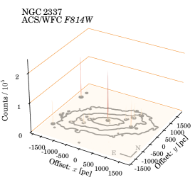
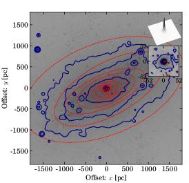
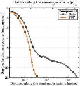
Figure 1: Nuclear star cluster (NSC) identification procedure using NGC 2337 as an example, based on the HST ACS/WFC $F814W$ data product. Left panel: Three-dimensional contour plot of NGC 2337 centered on the NSC. North is up and East is left. Contour lines represent the profile of a smoothed version of the data. For smoothing, we use a Gaussian kernel with standard deviation of five pixels. The NSC is the brightest source connected to the galaxy. Middle panel: Two-dimensional contour plot of the same data as in the left panel keeping the same orientation and blue contour lines. Red dashed lines give elliptical isophotes which were fit to the smoothed data; red points mark their centres. The two top right panels highlight the direct vicinity of the NSC. Right panel: One-dimensional surface brightness ($\mu_{F814W}$) plot of the elliptical isophotes (red colour, middle panel) as a function of semi-major axis ($a$) in both arcsecs and parsecs. Gray squares indicate the data. Orange squares show the extent of a TinyTim-generated PSF for the position of the NSC on the chip.

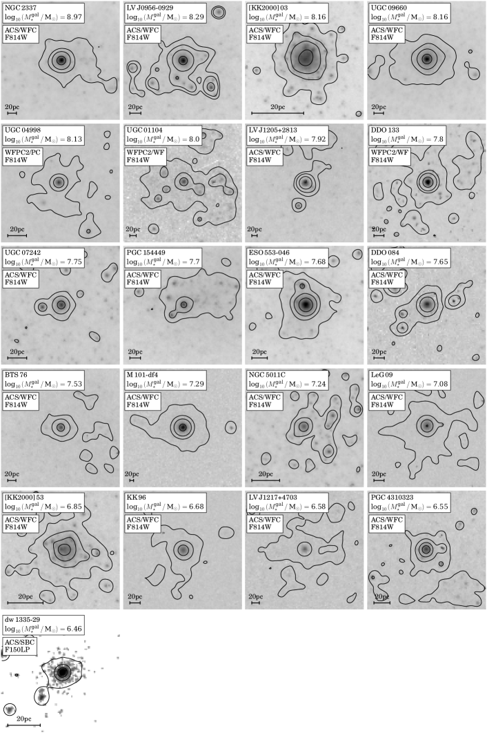
Figure 2: Collage of the $21$ newly discovered nuclear star clusters, sorted by host galaxy stellar mass from top left to bottom right. Each image shows a square box of side length $100\text{\,}\mathrm{pixels}$ centered on the nucleus; $20\text{\,}\mathrm{parsec}$ at the distance to the galaxies are indicated in each panel. North is up and East is left. The contour lines were derived from a smoothed version of the data using a Gaussian kernel with standard deviation of three pixels.

3 Analysis

3.1 Image processing

For each galaxy, we combined single exposures using flat-fielded data products obtained from the Hubble Legacy Archive (HLA). Instead of using the available final data products, we prefer to combine the exposures ourselves to ensure a homogeneous calibration process and to control the pixel scale of the drizzle output.

In a first step, we obtained the raw exposures from the ACS, WFPC2, and WFC3 instruments and updated the world coordinate system of each exposure using the latest reference files. This step was required to obtain a subpixel accuracy between individual exposures and to avoid a systematic broadening of the NSC. We fed the aligned exposures to AstroDrizzle (Gonzaga et al., 2012) which combined them into a single science product. No sky subtraction was performed. The program allows the user to modify the pixel fraction and pixel scale of the final drizzled image. The pixel fraction varies between zero and one where a value of zero corresponds to pure interlacing and a value of one to shifting and addition of pixel values from individual exposures. The drizzle algorithm (Fruchter & Hook, 1997) combines both techniques and enables a gain in image resolution and reduction in correlated noise. We chose a value of $0.75$ for the pixel fraction which is the smallest value for which no artifacts appeared in the weight map of the output image of AstroDrizzle. Increasing the value towards one did not change the fit results.

In addition to the pixel fraction, we changed the pixel scale for the ACS data products. The image resolution of the WFPC2 and WFC3 products remain unchanged. The limiting factor in increasing the spatial resolution of our ACS data products is given by the extent of the core of the theoretical PSF. This value is presented for the F550M band in the ACS manual. We determine the width of the PSF in a different filter by constructing the ratio of the full-width-half-maximum between TinyTim-generated PSFs in that filter and the F550M band. The pixel scale of the ACS images was chosen to Nyquist sample the PSF full-width-half-maximum at each wavelength. It ranges between $0.0415\text{\,}\mathrm{arcsec}\text{\,}{\mathrm{pixel}}^{-1}$ and $0.0472\text{\,}\mathrm{arcsec}\text{\,}{\mathrm{pixel}}^{-1}$, depending on the filter. The final resolution of each data product is indicated in Appendix B in Appendix B.

Finally, to perform the actual fit, we selected a square region of side length 100 pixels around the position of the NSC. Depending on the image resolution and the distance to the galaxy, this square region covers an area between $$\sim 50\text{\,}\mathrm{parsec}$\times$\sim 50\text{\,}\mathrm{parsec}$$ and $$\sim 500\text{\,}\mathrm{parsec}$\times$\sim 500\text{\,}\mathrm{parsec}$$. As NSCs typically have effective radii of a few parsecs (e.g. Neumayer et al., 2020) the selected area ensures that the wings of the NSCs are well captured. Nevertheless, we verified that both doubling the side length of the square and reducing it down to 60 pixels does not affect the final results.

3.2 PSF generation

Detailed knowledge of the PSF at the location of the NSC is required to reliably measure effective radii as they are generally compact and cover only a few pixels on the exposure. The PSF can be recovered from stellar sources in the image or generated synthetically. We decide to generate synthetic PSFs using TinyTim for three reasons:

• It is difficult to find non-saturated stars in the proximity of the NSC. Stars far away from the NSC should not be used as the HST PSFs vary significantly across the chip.

• The extracted PSF from stars may be subject to variations due to the positions of the stars on the chip and their stellar type.

• Extracting a PSF from stars results in an inhomogeneous treatment of using PSFs across the whole NSC sample.

Synthetic PSFs avoid these issues and allow us to control the input parameters such as position on the chip and the assumed stellar type.

To generate a PSF, we first determined the position of the NSC on each exposure. PSFs were generated using TinyTim and the location of the NSC on the chips, while assuming a G2V spectral type ($V-I=$0.71\text{\,}\mathrm{mag}$$) for the artificial star. After the PSF generation, we created a copy of the science exposures and subtract the image data from the first header file. The PSF was then added to the flattened image data at the previous location of the NSC. We then fed the data to AstroDrizzle and executed the program with the same settings as for the science data. This step ensures that the final PSF, which was extracted from the output of the program, is processed in the same way as the NSC on the science data.

Note that the inclusion of the AstroDrizzle processing step is crucial as the resulting PSF will change depending on the chosen parameter settings. In our tests the core of the resulting PSFs were slightly larger than the core of any of the TinyTim-generated PSFs. Therefore, not performing this step results in systematically larger effective radii compared to their ‘true’ values. We discuss this effect and other potential systematic uncertainties, such as the spectral type of the artificial star or the uncertainty on positioning the PSFs on the chips in Section A.2.

3.3 Fitting procedure

We assume that the NSC light distribution can be accurately modelled with a single Sérsic profile (Sérsic, 1968), as is common practice in the literature (e.g. Turner et al., 2012; Baldassare et al., 2014; Carson et al., 2015; Pechetti et al., 2020). For the background light, which includes the galaxy itself, we used a flat background assuming that local flatness holds in the proximity of the NSC. The only two exceptions are UGC 01104 and UGC 09660 where the fit required a second Sérsic profile for the underlying galaxy. Using version 1.8.0. of Imfit, the Sérsic profile was convolved with the PSF and fit to the data where the goodness of fit is evaluated via standard $\chi^{2}$ statistics. The data were fit using a differential evolution solver with Latin hypercube sampling (Storn & Price, 1997). The solver is less prone to be stuck in local minima compared to other solvers available in Imfit and does not rely on initial parameter estimates as parameter values are randomly sampled given lower and upper boundaries. We list the chosen boundary values in Table 1 and note that they are kept the same for all NSCs in all filters.

We additionally tested that other model functions do not significantly change the resulting parameter estimates. For the NSC, the tests included a King profile, multiple Sérsic profiles, point sources, nuclear rings, and various combinations. According to the Bayesian Information Criteria, none of these fits significantly improved over a fit with a single Sérsic profile. In addition, by adding a Sérsic profile to the flat background component to account for the underlying galaxy, we found that the assumption of local flatness is justified. We verified that using Cash statistics instead of the classical $\chi^{2}$ statistics does not change the results. We defer to Section A.2.1 for a detailed discussion regarding the choice and justification of these models.

For each NSC, the fits in different filters were performed independently of each other. However, in some cases the Sérsic index diverged towards the upper boundary in one filter, but not in the other. In these cases (BTS 76, DDO 084, ESO 553-046, [KK2000] 53, KK 96, LeG 09, LV J1217+4703, NGC 5011C), we kept all structural parameters of the fit with the diverging Sérsic index fixed such that only the $(x,y)$ position, the intensity at the effective radius, and the flat background component were allowed to vary.

For a number of galaxies the Sérsic index diverged towards high values in all available filters. This behaviour persisted when considering a single point source or a point source in combination with a Sérsic profile, and also occured independently of the settings chosen for AstroDrizzle, TinyTim, and Imfit. As the NSCs are more extended than the PSFs, no explanation for the diverging Sérsic index could be determined. To quantify the extent of the affected NSCs, we fixed the Sérsic index to a value of $n=2$. The choice of this value was motivated by the recent work of Pechetti et al. (2020) who classified their fits into three categories. NSCs which could be fit ‘well’ (their ‘Quality 0’ fits) have a mean / median value of $n=1.9\,/\,2.9$. Although six out of their 17 NSCs have $n>3$, we decided to set $n=2$ and to determine a systematic uncertainty based on fits using $n=0.5$ and $n=3$. In the parameter range $n\in[0.5,3.0]$, the Sérsic index does not correlate with the effective radius, allowing us to put constraints on it. For larger Sérsic indices, the effective radius also increases in a non-linear way. We give more details and discuss this choice further in Section A.2.3. However, it will become evident in Section 4 that the key results of this paper remain unchanged.

Table 1: Parameters and their boundaries supplemented to Imfit. The same values are used for all galaxies and filters.

Parameter	Boundary	Unit	Description
$x_{0}$	$[45,\,55]$	$\mathrm{pixel}$	NSC position
$y_{0}$	$[45,\,55]$	$\mathrm{pixel}$	NSC position
PA	$[-359.99,\,359.99]$(a)	$\deg$	Position angle
$\epsilon$	$[0.00,\,0.99]$	–	Ellipticity
$n$	$[0.00,\,15.00]$	–	Sérsic index
$r_{\mathrm{eff}}$	$[0.00,\,50.00]$	$\mathrm{pixel}$	Effective radius
$I_{\mathrm{eff}}$	$[0.00,\,I_{\mathrm{max}}]$(b)	counts	Intensity at $r_{\mathrm{eff}}$

• Often the fit was stuck at a boundary of $0\text{\,}\mathrm{\SIUnitSymbolDegree}$, hence the extension towards negative values. If the best fit position angle was negative, we added $180\text{\,}\mathrm{\SIUnitSymbolDegree}$ (twice) until it became positive.

• $I_{\mathrm{max}}$ is the peak intensity of the nuclear star cluster.

3.4 Nuclear star cluster stellar mass

Integrating Equation 1 over the radial component while assuming an ellipticity ($\epsilon$) yields the total intensity of the NSC ($L$) as

$$L=2\pi(1-\epsilon)r_{\mathrm{eff}}^{2}I_{\mathrm{eff}}\times\frac{n\,\mathrm{e}^{b_{n}}}{(b_{n})^{2n}}\times\Gamma(2n)\quad.$$ (2)

Combining $L$ with the zeropoint magnitudes and exposure times, which are both given in Appendix B, allows the calculation of apparent magnitudes.

We derived stellar masses using the $V-I$ colour and, therefore, converted from HST magnitudes to the $BVRI$ system. Following the approach by Pechetti et al. (2020), magnitudes were converted using different synthetic transformation. For the ACS/WFC data, the magnitudes were transformed using Table 22 and Equation 12 of Sirianni et al. (2005). WFPC2/WF and WFPC2/PC magnitudes were converted using Table 4 and Equation 16 of Dolphin (2009).

Once the magnitudes were transformed, we corrected them for Galactic extinction using a recalibrated version of the Schlegel et al. (1998) dust maps (Schlafly & Finkbeiner, 2011) and assuming the reddening law of Fitzpatrick (1999) with $R_{V}=3.1$. The corrected apparent magnitudes were then used to determine absolute magnitudes via the galaxy distance estimates and the absolute magnitude of the Sun. All extinction corrected apparent magnitudes are presented in Appendix B.

The stellar mass-to-light ratio relies on the $I$-band luminosity and $(V-I)_{0}$ colour and is identical to the one used in Pechetti et al. (2020). This relation ($M_{\star}/L_{I}$) is based on the work of Roediger & Courteau (2015) and reads

$$\log_{10}M_{\star}/L_{I}=-0.694+1.335\times(V-I)_{0}\quad,$$ (3)

where the slope and intercept have been determined by fitting a linear relationship to the underlying data which was provided by Joel Roediger (private communication).

The uncertainty on the NSC stellar masses are dominated by the uncertainty on the mass-to-light ratio which we assume to be $0.3\text{\,}\mathrm{dex}$ (Roediger & Courteau, 2015). Other uncertainties, which have been included via Gaussian error propagation, include the statistical and systematic uncertainties of the fit (see Appendix A), the uncertainty on the absolute magnitude of the Sun (assumed to be $0.04\text{\,}\mathrm{mag}$), and the uncertainty on the distance estimates. All quoted uncertainties give the $1\sigma$ interval. The resulting parameter values and their uncertainties are presented in Appendix B.

4 Results

In total, we derive NSC structural parameters for $19$ objects. In the case of dw 1335-29, the signal-to-noise ratio of the ACS/SBC F150LP data were to low to allow for an accurate determination of NSC parameters. In the case of PGC 154449, we could not determine parameter estimates from either the ACS WFC F606W or F814W data as the effective radius was approaching the boundary of $50\text{\,}\mathrm{pixels}$ in all attempts. We changed the size of the fitting region, the fitting routine, and applied various masks without achieving a stable fit result. For UGC 01104, structural parameters could not be determined in the ACS/WFC F300W band.

Furthermore, we derive colours and stellar mass estimates for $17$ objects. The blue colour estimate of ESO 553-046 [$(V-I)_{0}\sim$-3.2\text{\,}\mathrm{mag}$$, cf. Appendix B] leads to an unreliable estimate of the NSC mass. As no structural parameters could be estimated in two filters for dw 1335-29, PGC 154449, and UGC 01104, we do not derive NSC stellar masses. Finally, the stellar mass-to-light ratio of four NSCs is unreasonably high ($M_{\star}/L_{I}\gtrsim 4\mathrm{M}_{\odot}/\mathrm{L}_{\odot}$). These data points are excluded from the surface brightness and mass density profiles (cf. Section 4.4) and the determination of the scaling relation between NSC and host galaxy stellar mass (cf. Section 4.5).

4.1 Literature data

We compare our results to other NSCs in the Local Volume, in massive late-type field galaxies, and in dwarf ellipticals in the core of the Virgo cluster. For the Local Volume, we selected all known nucleated galaxies and obtained their NSC parameters, where available, from the most recent literature reference identified by Hoyer et al. (2021, their Table D1). For NSCs in massive late-type field galaxies, we used the data tables of Georgiev & Böker (2014). As the authors do not provide stellar masses, and to avoid systematic differences to our approach, we adopted their F606W and F814W apparent magnitudes and repeated the steps outlined in Section 3.4. Table 5 of Sánchez-Janssen et al. (2019) provides stellar masses for NSCs in dwarf ellipticals in the core of the Virgo cluster. In addition, we adopt the data from Carlsten et al. (2022) for dwarfs around massive late-type field galaxies. We compare to Galactic globular clusters using the data from Harris (1996) and Baumgardt & Hilker (2018).

We present an overview of the parameters of other NSCs in Local Volume galaxies in Appendix B. NSC stellar masses for the sample of Georgiev & Böker (2014) are presented in Appendix B.

Galaxy stellar masses were adopted from Hoyer et al. (2021) for the whole Local Volume data set and the galaxy sample of Georgiev & Böker (2014). We take galaxy stellar masses for dwarf ellipticals in the core of the Virgo cluster from Table 4 of Sánchez-Janssen et al. (2019).

4.2 Wavelength dependence

We investigate whether NSC structural parameters are wavelength dependent by comparing differences in parameter estimates between the most commonly available F660W and F814W bands. Within the uncertainties, we find no significant differences in both $\epsilon$ and $r_{\mathrm{eff}}$. The position angle changes insignificantly ($\Delta\mathrm{PA}\lesssim$30\text{\,}\mathrm{\SIUnitSymbolDegree}$$) for most NSCs.

4.3 Structural properties

Here we investigate the structural properties of the new detections using the F814W band. We compare to other data from the Local Volume and Georgiev & Böker (2014) using the same band, if available. In addition, we compare to the globular cluster population of the Milky Way (Baumgardt & Hilker, 2018; Harris, 1996).

Panel A of Figure 3 shows the ellipticity versus NSC stellar mass. Most of the new detections have $\epsilon\sim$0.1$$ but at most $\sim$0.3$$. With the exception of the most massive NSCs, both the stellar mass and ellipticity compare to Milky Way GCs. The overall increase of ellipticity with increasing mass is in agreement with Figure 24 of Spengler et al. (2017). The new detections reveal that this trend does not continue down to the lowest mass clusters, as suggested by the few existing Local Volume data points from the literature. Similarly, the GC population of the Milky Way does not show a correlation as well.

Panel B shows the effective radius versus NSC mass. The new detections occupy the low-mass and compact-size region in the parameter space. While at higher NSC mass there exists a correlation between the effective radius and NSC mass (e.g. Georgiev & Böker, 2014; Georgiev et al., 2016; Neumayer et al., 2020), this relation appears to break down at $M_{\star}^{\mathrm{nsc}}\sim${10}^{6}\text{\,}\mathrm{M_{\odot}}$$, as revealed by the new detections. The distribution of Galactic GCs overlap with the new detections, corroborating a tight connection between both types of systems in this mass range. Furthermore, the new detections appear to follow the same trend as the GCs by increasing in effective radius with decreasing mass.

There exist six data points with $r_{\mathrm{eff}}\geq$10\text{\,}\mathrm{pc}$$ and $M_{\star}^{\mathrm{nsc}}\leq${10}^{6}\text{\,}\mathrm{M_{\odot}}$$, which partially overlap with the distribution of Galactic GCs but are otherwise outliers from the NSC distribution. If the NSCs truly reside in this part of the parameter space, one explanation could be that their evolution is similar to that of the NSC of the Pegasus dwarf galaxy: the cluster initially formed in the centre of their host galaxy, was relocated outside of the central region where $r_{\mathrm{eff}}$ increased due to the weaker tidal field, and migrated back towards the centre (Leaman et al., 2020). For both UGC 08638 and NGC 4163, this mechanism could still be in process as the projected distance of the NSC to the photometric centre is $\sim 480\text{\,}\mathrm{pc}$ and $\sim 150\text{\,}\mathrm{pc}$, respectively (Georgiev et al., 2009). The projected distance of the other two galaxies (KK 197 and ESO 269-066) is close to $0\text{\,}\mathrm{pc}$ (Georgiev et al., 2009).

Panel C of Figure 3 shows the Sérsic index versus effective radius. There appears to be a trend in that the index drops from $n\sim 7$ to $\sim 1$ when the effective radius increases from $r_{\mathrm{eff}}\sim$1\text{\,}\mathrm{pc}$$ to $\sim$10\text{\,}\mathrm{parsec}$$. However, multiple NSCs occupy the high Sérsic index and high effective radius parameter space, questioning a potential universal correlation. More data and further studies are required to explore this parameter space.

Panel D shows the previously identified weak relationship between the logarithmic Sérsic index and NSC stellar mass by Pechetti et al. (2020). We add the new detections to the figure and fit the combined data sets with a linear function. The best fitting relation reads

$$\log_{10}\,n_{F814W}=0.52^{+0.50}_{-0.38}-0.20^{+0.53}_{-0.29}\times\log_{10}\frac{M_{\star}^{\mathrm{nsc}}}{${10}^{6}\text{\,}\mathrm{M_{\odot}}$}\;.$$ (4)

The parameters differ significantly from the values found by Pechetti et al. (2020) and question the presence of a tight correlation. Therefore, while the Spearman correlation coefficient evaluates the trend as significant ($p=0.015$), we recommend against using the Sérsic index relation to parameterise NSCs.

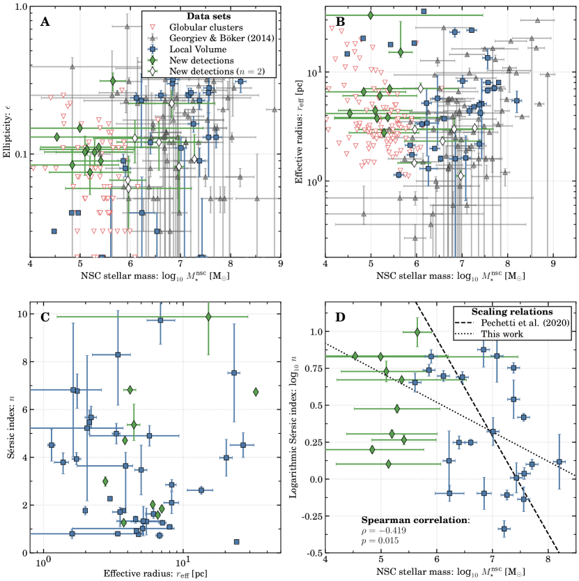
Figure 3: Panel A: Ellipticity ($\epsilon$) versus nuclear star cluster (NSC) stellar mass ($M_{\star}^{\mathrm{nsc}}$). We compare the new detections (green diamonds) to NSCs in massive late-type spirals (Georgiev & Böker, 2014), a compilation of NSCs in the Local Volume, and Galactic globular clusters (Harris, 1996; Baumgardt & Hilker, 2018). The new detections are split into two categories, depending on whether the Sérsic index ($n$) needed to be fixed at $n=2$. Panel B: Effective radius ($r_{\mathrm{eff}}$) versus NSC stellar mass. The markers and color are the same as in panel A. Panel C: Sérsic index versus effective radius. The data from Georgiev & Böker (2014) and Harris (1996); Baumgardt & Hilker (2018) are not available as the clusters were modelled with King profiles. Most of the Local Volume data come from Pechetti et al. (2020). Panel D: Sérsic index versus NSC stellar mass. A dashed black line gives the weak scaling relation identified by Pechetti et al. (2020). The dotted line gives the best-fit linear relation including the new detections. The Spearman correlation index $\rho$ and its associated $p$-value of thew new fit are given in the lower left corner.

4.4 Surface brightness & surface mass density profiles

Combining the effective radius and stellar mass, we determine a mean surface density for the new detections. We show this parameter space in Figure 4, comparing the new detections with literature data from Norris et al. (2014) and Neumayer et al. (2020) for other NSCs, and with Baumgardt & Hilker (2018) for Milky Way GCs. For the newly detected NSCs, we fit the correlation using a linear function to find

$$\log_{10}\,\Sigma_{\mathrm{eff}}=-2.72^{+0.61}_{-0.71}+1.13^{+0.13}_{-0.12}\times\log_{10}\,M_{\star}^{\mathrm{nsc}}\;,$$ (5)

where the parameter values are determined through ${10}^{5}$ bootstrap iterations. We note that although some of NSCs at $M_{\star}^{\mathrm{nsc}}\sim${10}^{8}\text{\,}\mathrm{M_{\odot}}$$ seem to follow this relation as well, their overall distribution get wider and seems to flatten. At the low-mass end, the newly detected NSCs overlap again with Galactic GCs. Note that about $65\text{\,}\mathrm{\char 37\relax}$ of these GCs fall above the best-fit relationship.

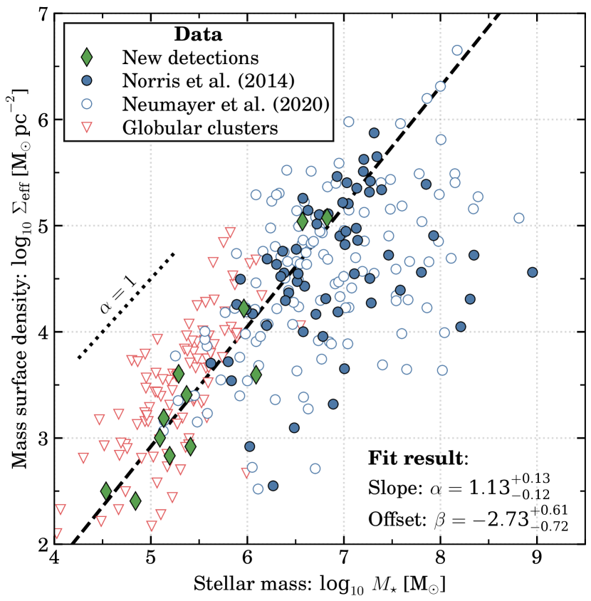
Figure 4: Mean stellar mass surface density within the effective radius ($\Sigma_{\mathrm{eff}}$) versus cluster mass ($M_{\star}$). We compare the new detections (green diamonds) to other nuclear star clusters from Norris et al. (2014) and Neumayer et al. (2020), and to Milky Way globular clusters (Baumgardt & Hilker, 2018). The best-fit values of a linear relationship fit to the new detections, as determined through ${10}^{5}$ bootstrap iterations, are indicated in the lower right corner.

Next, we explore the surface brightness of the star clusters. Panel A of Figure 5 shows the surface brightness as a function of radius where the profiles relate to the Sérsic model fits from the F814W band. To highlight uncertainties, we plot the profiles of $100$ out of $500$ bootstrap iterations, which we used to determine statistical uncertainties (cf. Section A.1). Each set of profiles is colour-coded based on the host galaxy stellar mass.

Similarly, panel B shows the surface mass profile versus radius. We convert the profiles to stellar mass by using the mean colour of the NSCs. Note the assumption that the mass-to-light ratio is radially constant, which is not the case for higher mass NSCs in other Local Volume galaxies (e.g. Carson et al., 2015) and the Milky Way NSC (Feldmeier-Krause et al., 2015; Feldmeier-Krause et al., 2017). However, as a function of wavelength, the size or ellipticity does not differ significantly for the new detections and, therefore, using the mean colour likely provides a decent estimate of their average stellar populations. The colour-coding of the profiles is the same as in panel A.

From both figures it becomes apparent that the surface brightness of the clusters positively correlates with the host galaxy stellar mass. To quantify this observation further, we show the surface mass profiles evaluated at the clusters’ effective radii versus the host galaxy and NSC stellar masses in Figure 6. According to the Spearman correlation coefficients, we find a clear correlation between both quantities. A fit using a linear relationship yields

$$\log_{10}\,\mu=\begin{cases}1.13^{+0.16}_{-0.14}-5.3^{+1.0}_{-1.0}\times\log_{10}\,M,\quad\mathrm{for}\;M=M_{\star}^{\mathrm{gal}}\\ 1.29^{+0.10}_{-0.12}-4.05^{+0.62}_{-0.62}\times\log_{10}\,M,\quad\mathrm{for}\;M=M_{\star}^{\mathrm{nsc}}\;,\end{cases}$$ (6)

where the uncertainties are determined with ${10}^{5}$ bootstrap iterations. Note that the slope value for the relation using the NSC mass is steeper than one. This is related to both the NSC versus host galaxy stellar mass relation (cf. Section 4.5 below) and the observation that the effective radius decreases with increasing NSC mass for the new detections (cf. Figure 3, panel B).

From both panels it is apparent that BTS 76 does not follow the relationship and was excluded from both fits. Compared to other NSCs, the effective radius of this nucleus is significantly larger. As discussed in Section 4.3, the NSC sub sample with large effective radii and low stellar masses may have evolved differently from the other clusters: if the cluster relaxes in a weaker tidal field (i.e. the outskirts of the host galaxy), its central density may drop while the total mass of the cluster remains roughly the same.

Note that Pechetti et al. (2020) investigated the three-dimensional density of high-mass NSCs in higher-mass galaxies finding a similar trend: the NSC density positively scales with the host galaxy stellar mass. Our data show that such a correlation appears to continue down to lower galaxy and NSC stellar masses, effectively extending the existence of a relation from $\log_{10}\,M_{\star}^{\mathrm{gal}}/\mathrm{M}_{\odot}\sim 11$ to $\log_{10}\,M_{\star}^{\mathrm{gal}}/\mathrm{M}_{\odot}\sim 6.5$.

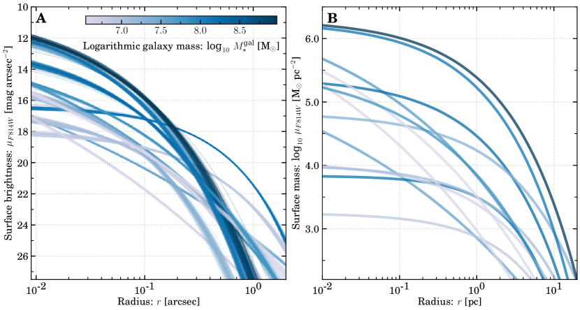
Figure 5: Panel A: Surface brightness in the F814W band ($\mu_{\mathrm{\textit{F814W}}}$) versus radius ($r$) of the newly detected nuclear star clusters (NSCs). The profiles give the Sérsic models fit to the data. To highlight uncertainties, we show $100$ profiles for each NSC, randomly drawn from a total of $500$ bootstrap iterations. Each set of profiles is colour-coded by the stellar mass of the host galaxy where a darker colour corresponds to a more massive galaxy. Panel B: Surface mass density based on the F814W band versus radius. The conversion from the best-fit surface brightness profiles to mass profiles assumes a radially constant mass-to-light ratio. This assumption is invalid in higher-mass NSCs (Carson et al., 2015; Feldmeier-Krause et al., 2015; Feldmeier-Krause et al., 2017), which is why we show only a single profile for each NSC. The colour of the lines is the same as in panel A.

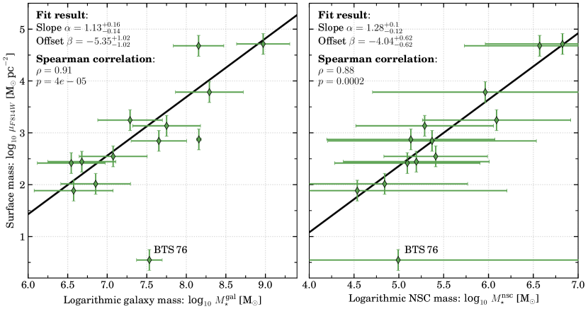
Figure 6: Surface mass profile evaluated at the nuclear star clusters effective radius versus host galaxy (panel A) and cluster stellar mass (panel B). Solid lines give the best-fit linear relation ($\log_{10}\,\mu=\alpha+\beta\times\log_{10}\,M_{\star}$) whose parameters, as determined through ${10}^{5}$ bootstrap iterations, are indicated in the panels. In addition, we show the Spearman correlation parameter ($\rho$) and its associated $p$-value. BTS 76, as indicated, does not fit the overall trend and was excluded from the fits.

4.5 NSC stellar mass versus galaxy stellar mass

In this section we investigate the scaling relation between the NSC stellar mass and its host stellar mass. We combine literature data of the Local Volume, Georgiev & Böker (2014), and Carlsten et al. (2022) with our new detections to gain statistical significance. To this combined data set, we fit the function

$$\log_{10}\,M_{\star}^{\mathrm{nsc}}=\alpha\times\log_{10}\,\frac{M_{\star}^{\mathrm{gal}}}{${10}^{9}\text{\,}\mathrm{M_{\odot}}$}+\beta\quad,$$ (7)

which has also been used previously (Georgiev et al., 2016; Neumayer et al., 2020). To fit the data, we use the scipy implementation of the orthogonal distance regression, which takes into account uncertainties on both axes (see also Boggs & Rogers, 1990). The uncertainty on the stellar masses of literature data are assumed to be $0.3\text{\,}\mathrm{dex}$ if no value is provided. As the slope $\alpha$ of the relation in Equation 7 seems to steepen for galaxies above $M_{\star}^{\mathrm{gal}}\sim$e9.5\text{\,}\mathrm{M_{\odot}}$$ (Georgiev et al., 2016; Neumayer et al., 2020), we restrict the fit to $M_{\star}^{\mathrm{gal}}<$e9.5\text{\,}\mathrm{M_{\odot}}$$. Furthermore, from the fit we removed four NSCs (DDO 133, LV J1205+2813, NGC 5011C, and UGC 04998) as they have high stellar mass-to-light ratios ($M_{\star}/L_{I}\gtrsim 4\mathrm{M}_{\odot}/L_{\odot}$). The final uncertainties of the fit were determined via ${10}^{5}$ bootstrap iterations.

Figure 7 shows the data set as well as the best-fit relationship for which we find $\alpha=0.82^{+0.08}_{-0.08}$ and $\beta=6.68^{+0.13}_{-0.13}$. This slope is steeper than what was found by Neumayer et al. (2020, $\alpha\sim 0.48$) who used data from various publications and a mix of environments. Restricting the fit to the high-mass end yielded a value of $\alpha\sim 0.92$, which agrees with a previously reported value (Georgiev et al., 2016) and our value.

Our results and the observation that the fit by Neumayer et al. (2020) is dominated by dwarfs in a dense cluster environment [Virgo (Sánchez-Janssen et al., 2019) and Fornax (Ordenes-Briceño et al., 2018)] could suggest that the environment of the dwarf galaxies plays a role in the NSC versus host stellar mass relationship. To test this hypothesis, we add the data set of Sánchez-Janssen et al. (2019), exploring the relationship for dwarfs in the core of the Virgo galaxy cluster. Only considering their data, we find $\alpha=0.55^{+0.06}_{-0.05}$ and $\beta=6.69^{+0.10}_{-0.09}$ using again ${10}^{5}$ bootstrap iterations. As expected, the slope is comparable to the value found by Neumayer et al. (2020) but significantly smaller than the value for dwarfs in the field.

To check whether the origin for the difference between environments stems from the lowest mass galaxies, we repeat the fit to the Virgo cluster data set forcing $M_{\star}^{\mathrm{gal}}\geq$e6.5\text{\,}\mathrm{M_{\odot}}$$. This results in $\alpha=0.70^{+0.08}_{-0.07}$ and $\beta=6.83^{+0.13}_{-0.11}$. As the slope is now comparable to the one found for the field environment we conclude that the low-mass galaxies in the Virgo cluster, which host more massive NSCs than in the field, are responsible for environmental trends.

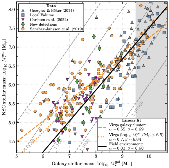
Figure 7: Nuclear star cluster (NSC) stellar mass ($M_{\star}^{\mathrm{nsc}}$) versus host galaxy stellar mass ($M_{\star}^{\mathrm{gal}}$) for the new detections (greend diamonds), a compilation of Local Volume data (blue squares), massive late-type galaxies in the field (Georgiev & Böker, 2014; gray up-pointing triangles), dwarf galaxies around massive late-types (Carlsten et al., 2022; purple down-pointing triangles), and dwarfs in the core of the Virgo galaxy cluster (Sánchez-Janssen et al., 2019; orange circles). Uncertainties are omitted for clarity. The combined data of new detections, other Local Volume, and field galaxies are fit with a linear relationship, such that $\log_{10}\,M_{\star}^{\mathrm{nsc}}=\alpha\log_{10}\,(M_{\star}^{\mathrm{gal}}\,/\,${10}^{9}\text{\,}\mathrm{M_{\odot}}$)+\beta$. This relationship is shown with a black solid line; its best-fit parameters are indicated in the bottom right. A gray shaded area gives the region excluded from the fit. Furthermore, from the fit we exclude four NSCs (DDO 133, LV J1205+2813, NGC 5011C, and UGC 04998) which have a high stellar mass-to-light ratio, but still show the data points in the figure. Uncertainties are determined thorugh ${10}^{5}$ bootstrap iterations. For dwarfs in the core of the Virgo cluster, we perform the same fit and show the best-fit relation with a dashed orange line. The slope of $\alpha\sim 0.55$ is significantly below the value found for dwarfs in the field. Restricting the fit to galaxies in Virgo to $M_{\star}^{\mathrm{gal}}\geq$e6.5\text{\,}\mathrm{M_{\odot}}$$ (orange dotted) line results in a slope with agrees with the one for the field environment within the $1\sigma$ interval.

5 Discussion

We presented a comparison between the Milky Way GCs and the newly detected NSCs in the previous sections and argue in Section 5.1 that dissipationless GC migration is the main formation scenario for NSCs in low-mass dwarf galaxies. Afterwards, in Section 5.2, we discuss whether the NSCs are a merger product of multiple GCs or whether they are not.

5.1 Formation scenario

NSCs are believed to form via two mechanisms: at the low-mass end, GC migration appears to dominate the formation of NSCs (e.g. Tremaine et al., 1975; Hartmann et al., 2011; Antonini et al., 2015; Fahrion et al., 2022a) and in-situ star formation contributes only a small part to the mass budget, if at all. With increasing galaxy stellar mass in-situ star formation gains importance (e.g. Turner et al., 2012; Sánchez-Janssen et al., 2019; Neumayer et al., 2020) and will eventually dominate over the GC migration scenario (Fahrion et al., 2021; Fahrion et al., 2022b).

We compared the structural properties of the newly detected NSCs with Milky Way GCs in Figures 3 and 4 finding a similarity between both systems. More specifically, the ellipticity, effective radius, stellar mass, and surface density of many of the new detections matches the distribution of Milky Way GCs. As speculated in the literature already (e.g. Miller & Lotz, 2007; Sánchez-Janssen et al., 2019), this is a direct hint that the dissipationless GC migration scenario is the main formation mechanism of these NSC.

We also found that the ellipticity remains roughly constant below $M_{\star}^{\mathrm{nsc}}\sim$e6.5\text{\,}\mathrm{M_{\odot}}$$ and starts to increase for higher mass clusters. An increase in ellipticity hints towards in-situ star formation as the in-falling gas is expected to form stars in a flattened disk due to its angular momentum. In observations, such a flattening has been observed in combination with young stellar populations in edge-on spiral galaxies (e.g. Seth et al., 2006). In simulations, Hartmann et al. (2011) showed that NSCs, which formed through repeated GC mergers, typically are not very flattened. Crucially, as we show in Figure 8 the measured ellipticity of the NSCs does not depend on the inclination of the host galaxy at all stellar masses.

As shown in Figure 7, the NSC versus host galaxy stellar mass correlation appears to be affected by host environment with cluster members typically hosting more massive NSCs than field galaxies. We found that the difference is greatest at the low-mass end $M_{\star}^{\mathrm{gal}}\leq$e6.5\text{\,}\mathrm{M_{\odot}}$$ and becomes insignificant towards higher masses. If in-situ star formation is unimportant at the lowest galaxy stellar masses, the difference in NSC must arise from differences in the progenitor GCs.

There appear two possibilities to generate more massive NSCs:

• The NSCs in dwarfs in dense environments experienced more GC merger events than NSCs in a field environment, elevating their masses. We discuss this option further in Section 5.2.

• The difference in mass does not arise from a significant difference in mergers but from a difference in progenitor GC mass.

The argument that the progenitor GC is more massive in a dense environment relies on GC formation scenarios. The cluster formation efficiency (Bastian, 2008) positively correlates with the surface density of star formation (see Stahler, 2018, and references therein) and leads to an elevated mass fraction of stars in clusters. From observations it appears that this effect results in an increased number of GCs in present-day dwarf galaxies in galaxy clusters (e.g. Peng et al., 2008) and not in differences in the GC mass function (Carlsten et al., 2022). The GC luminosity function appears to be roughly equivalent between the environments (Figure 7 in Carlsten et al., 2022) but this may not be the case at high redshift (e.g. Parmentier & Gilmore, 2007; Kruijssen & Cooper, 2012).

If the GC mass function remains unchanged between environments at the time when the NSC formed, the NSC’s mass may still be elevated due to the higher number of GCs produced in a dense environment. When drawn from the same distribution, a higher number of GCs correspond to a higher probability that the most massive GC in a galaxy in a dense environment is more massive than its counterpart in a galaxy in a loose environment.

We note that the differences in NSC stellar mass found at the low-mass end could also be related to selection bias. Our data rely on a catalogue of galaxies in the Local Volume (see Karachentsev et al., 2013, and references therein) while the Virgo cluster data of Sánchez-Janssen et al. (2019) relies on a uniform set of imaging data (Ferrarese et al., 2012). The data of Carlsten et al. (2022) indicate that satellites around massive field galaxies, where a significant mass fraction is contained by the NSC, do exist but in fewer numbers than in the Virgo cluster. Whether this is also a selection effect is unclear. Note that it appears unlikely that higher-mass galaxies were stripped by $\sim$1\text{\,}\mathrm{d}\mathrm{e}\mathrm{x}$$ in mass in the galaxy cluster while the NSC mass remains unchanged (e.g. Smith et al., 2016).

Truncated star formation during the galaxy infall may lead to a bias in the NSC versus galaxy mass relationship as well: asynchronous formation timescales of the NSC and its host galaxy leads to a higher cluster mass fraction if most cold gas is removed during infall. This effect could partly be responsible for both the observed environmental dependence of the stellar mass correlation as well as a higher NSC occupation fraction in dense environments (Leaman & van de Ven, 2022). Whether this effect can fully explain the observed environmental dependence remains unclear.

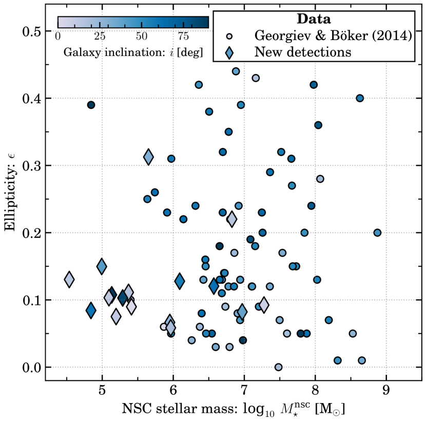
Figure 8: Ellipticity ($\epsilon$) versus nuclear star cluster stellar mass ($M_{\star}^{\mathrm{nsc}}$). We show the new detections (diamonds) and compare with NSCs in massive late-type galaxies (Georgiev & Böker, 2014). Each data point is colour-coded by the inclination of the host galaxy.

5.2 Are our newly detected NSCs merger products of GCs?

A second method for forming NSCs is the process of repeated GC mergers. As mentioned in the previous section, at fixed galaxy stellar mass, the number of GCs is higher in a dense environment than in the field. Therefore, a present-day NSC in a galaxy in a dense environment could have experienced more GC mergers than in a loose environment, explaining its increased mass at the low-mass end of galaxies.

One argument in favor of this scenario is shown in Figure 4. We found that $\sim$65\text{\,}\mathrm{\char 37\relax}$$ of GCs fall above the mass density versus cluster mass relation. Antonini et al. (2012) and Antonini (2013) showed that the merger product of two GCs results in an increase in effective radius of the merger product where $r_{\mathrm{eff}}\propto\sqrt{M_{\star}}$. If two clusters merge in the density versus mass parameter space, their mass will increase but the overall density will drop, meaning that the data point moves towards the bottom right part in Figure 4. Therefore, as the Milky Way GCs are, on average, denser at the same stellar mass than our new detections, NSCs could be a merger product of multiple progenitor GCs. However, given the uncertainties of the data points it is not possible to prove this scenario for individual objects.

If true in all environments, we would expect that the effective radius of NSCs in the core of the Virgo cluster are more extended than in the field environment, as they experienced more GC merger events. The data of the Next Generation Virgo Cluster Survey (Ferrarese et al., 2012) obtained with MegaCam (Boulade et al., 2003) have an effective resolution of $\sim$50\text{\,}\mathrm{pc}$$, prohibiting an analysis of the NSC sizes (Ferrarese et al., 2020).

In a pure dissipationless merger scenario, the steepness of the slope of the cluster may not exceed that of its progenitors (Dehnen, 2005). The slope of the density profiles is determined by evaluating $\mathrm{d}\log_{10}I/\mathrm{d}\log_{10}r$ from Equation 1 and converting to $\mathrm{d}\log_{10}M_{\star}/\mathrm{d}\log_{10}r$ and using the mass-to-light ratio,

$$\frac{\mathrm{d}\log_{10}\,M_{\star}^{\mathrm{nsc}}}{\mathrm{d}\log_{10}r}=-\frac{\log 10}{r_{\mathrm{eff}^{2}}}\frac{b_{n}}{n}\bigg{(}\frac{r}{r_{\mathrm{eff}}}\bigg{)}^{1/n}\;.$$ (8)

For the new detections, we find an increase in this slope but the trends are not significant. Based on a similar trend and a comparison to typical GC densities, Pechetti et al. (2020) concluded that in-situ star formation plays a key role in the formation and evolution of NSCs. For the majority of our clusters, it remains unclear whether in-situ star formation contributes to the mass budget at all. Fahrion et al. (2022a) showed that most of the mass fraction of NSCs in similar-mass galaxies comes from old, metal-poor stars but that in-situ star formation may still be present.

If low-mass NSC structure argues for GC merging as the primary formation channel, then at the highest NSC masses, we do see some evidence for in-situ formation The two highest-mass NSCs in our sample are denser than the densest GCs, including Milky Way clusters (e.g. McLaughlin & van der Marel, 2005; Baumgardt & Hilker, 2018), and many ultra-compact dwarfs (e.g. Norris et al., 2014). This hints towards a contribution of in-situ star formation, supported by Fahrion et al. (2022b) who found that in-situ star formation gains importance for $\log_{10}\,M_{\star}^{\mathrm{nsc}}/\mathrm{M}_{\odot}\gtrsim 6.5$ and may contribute $50\text{\,}\mathrm{\char 37\relax}$ of the NSCs mass. Whether these objects are a product of repeated GC mergers is plausible but remains unclear as the increase in profile slope may be caused by central in-situ star formation.

Combining all arguments, it appears to be clear that there is a fundamental connection between GCs and NSCs in these low-mass galaxies. Although likely, it remains unclear whether the lowest-mass NSCs are individual GCs, which experienced no merger events, or whether the NSCs are the product of GCs mergers. At least the two most-massive NSCs in our sample likely experienced in-situ star formation, elevating the steepness of their profile slopes and making them denser than any Milky Way GC.

6 Conclusions

In this work we presented an analysis of $21$ newly discovered nuclear star clusters (NSCs) in Local Volume galaxies using Hubble Space Telescope imaging data. We convolved a TinyTim-generated point spread function with a Sérsic profile to determine structural parameters. NSC stellar masses were determined based on integrated photometry in different filters.

The new detections are compact with a typical effective radius $r_{\mathrm{eff}}\lesssim$12\text{\,}\mathrm{pc}$$ and populate the lower stellar mass end of the whole NSC population at $M_{\star}^{\mathrm{NSC}}\lesssim${10}^{7}\text{\,}\mathrm{M_{\odot}}$$. We find that the correlation between $M_{\star}^{\mathrm{nsc}}$ and $r_{\mathrm{eff}}$ breaks down for the low-mass galaxies, as indicated by Georgiev et al. (2016). In addition to their compact size, the new detections have typically low- to moderate Sérsic indices ($n\lesssim 6$), which compares to other NSCs in the Local Volume. The linear relation between the ellipticity and the mass of the clusters break down below $M_{\star}^{\mathrm{gal}}\sim$e6.5\text{\,}\mathrm{M_{\odot}}$$ where the NSCs have ellipticies of $\epsilon\sim 0.1$. A comparison to Milky Way globular clusters (Harris, 1996; Baumgardt & Hilker, 2018) reveals that most of the newly detected NSCs have similar ellipticity, effective radius, and stellar mass, corroborating a relation between both types of clusters.

NSCs are the densest stellar systems (e.g. Walcher et al., 2005; Norris et al., 2014; Neumayer et al., 2020) and we find central surface brightness values ranging between $\sim 18$ and $\sim$12\text{\,}\mathrm{mag}\text{\,}{\mathrm{arcsec}}^{-2}$$ in the F814W band, corresponding to central surface masses of $\sim 3.2$ and $6.2\text{\,}\mathrm{M_{\odot}}\text{\,}{\mathrm{parsec}}^{-2}$, respectively. We find that both the surface brightness and stellar mass profiles correlate with both the NSC and host galaxy stellar mass. Furthermore, the slope of the profiles evaluated at their effective radii weakly correlates with both the NSC and host galaxy stellar mass. A similar trend for three dimensional slope values was observed by Pechetti et al. (2020) for more massive NSCs. Our data reveal that this trend continues down to the lowest-mass nucleated galaxies.

Similar to the surface brightness profiles, the average surface mass density within the effective radius correlates with NSC stellar mass as well. A linear fit reveals that some denser and more massive NSCs follow the same trend, albeit their distribution widens and flattens towards higher masses. Comparing to Milky Way globular clusters, we find that about $65\text{\,}\mathrm{\char 37\relax}$ fall above the best-fit relation. Again, most of the lowest-mass NSCs coincide with the distribution of Milky Way globular clusters.

We investigated the scaling relation of NSC versus host galaxy mass. A linear fit revealed that the nucleated dwarfs in a field environment have a steeper relationship ($\alpha=0.82^{+0.08}_{-0.08}$) than dwarfs in the core of the Virgo galaxy cluster ($\alpha=0.55^{+0.06}_{-0.05}$; Sánchez-Janssen et al., 2019). However, forcing $M_{\star}^{\mathrm{gal}}\geq$e6.5\text{\,}\mathrm{M_{\odot}}$$ for the fit results in a relationship with a steepness comparable to the value for dwarfs in the field environment ($\alpha=0.70^{+0.08}_{-0.07}$). Therefore, the environmental dependence in the $M_{\star}^{\mathrm{nsc}}$-$M_{\star}^{\mathrm{nsc}}$ relation is caused by the lowest-mass nucleated galaxies.

Our results reinforce the connection between globular clusters and nuclear star clusters. They also corroborate other studies in that globular cluster migration is the main formation mechanism in dwarf galaxies and that in-situ star formation gains importance with increasing mass (e.g. Neumayer et al., 2020).

We find a clear environmental dependence, such that in low-mass galaxies, the NSCs are fractionally more massive in denser environments. We argue this extra mass is most likely explained by a larger pool of available GCs for mergers, or even just for becoming the NSC. On the flip side, the high stellar density of our two most massive NSCs suggest that in-situ formation, rather than merging, dominated their growth. This interpretation fits well with other recent research, which shows that the in-situ fraction of a nuclear star cluster increases with increasing stellar mass (Fahrion et al., 2022b; Fahrion et al., 2022a). Our data cannot reveal whether there also exists an environmental dependence in the correlation between the NSCs’ in-situ fraction and stellar mass.

Data availability

The data underlying this article are available in the article and in its online supplementary material.

Appendix A Assessing uncertainties

In this section we discuss statistical and systematic uncertainties and how we determined them. If applicable, the final $1\sigma$ uncertainties in the data tables consist of the sum of the quadratic statistical and systematic uncertainties.

A.1 Statistical uncertainties

For each fit, we determine the statistical uncertainties via bootstrapping. During each iteration of bootstrapping Imfit generates a new data array where pixel values are resampled from the original data. The new data array is then fit using Levenberg-Marquardt minimisation to speed up the fit. We chose $500$ bootstrap iterations which resulted in a good-enough sampling of the confidence intervals; increasing the value to $2500$ iterations did not change the results.

The quoted uncertainties were determined by the $1\sigma$ distribution of the bootstrap results. However, to determine photometric parameter values and to convert the effective radius from pixels to parsecs, the uncertainties needed to be propagated forward. In the case of apparent magnitudes, we used the bootstrap distributions of all required parameter values to determine the total intensity of the NSC (cf. Equation 2). The uncertainty on the zeropoint magnitude is small compared to the uncertainty of the instrumental magnitude and was not taken into account. For the determination of colours, we used Gaussian error propagation by assuming that the distributions of apparent magnitudes follow a Gaussian distribution. We used the larger uncertainty of the asymmetric parameter distribution as the symmetric uncertainty of the assumed Gaussian-like distribution. For the apparent magnitudes, this choice seems to be justified, as shown by the symmetry of the uncertainties of the apparent magnitudes in Appendix B. Afterwards, we determined absolute magnitudes and stellar masses via Gaussian error propagation. The same scheme was applied to transform effective radii from pixels to parsecs.

A.2 Systematic uncertainties

To quantify systematic uncertainties in our work, we conducted various tests involving the choice of model functions and the programs AstroDrizzle and TinyTim. We will additionally discuss the correlation between the Sérsic index and the effective radius and the induced uncertainty by fixating the index in some of our fits. All fits were performed with Imfit and are independent of the chosen solver or fit statistic. Unless otherwise stated, we chose the data of NGC 2337 in the ACS/WFC $F814W$ band.

A.2.1 Model functions

We assumed that the NSCs can be represented well by a single Sérsic function but this choice is rather arbitrary. Complex substructures may be present in extragalactic NSCs but typically are unresolved given their distances and subsequent angular sizes on the HST instruments. Nevertheless, in some cases individual stars (e.g. [KK2000] 03) and extended emission around the NSC can be seen which are not well represented by a single Sérsic profile.

We repeated most fits using different model functions for the NSC. We chose a single King profile (King, 1962, 1966), a combination of a Sérsic profile and a point source, two Sérsic profiles where the second profile fits the extended emission, and two Sérsic profiles in combination with a point source. The addition of a point source to the fits was tested for all NSCs but did not yield different structural parameters. In most cases the intensity of the point source was insignificant compared to the intensity of the Sérsic profile at the effective radius, thus not adding significant flux to the total apparent magnitude.

Instead of using a Sérsic profile, we used a classical King profile to fit the NSC of LeG 09 in the ACS/WFC $F814W$ band. The boundaries for the core and tidal radii were set to $[0.01,10]$ and $[0.01,50]$. Fitting LeG 09 with a Sérsic profiles and using $500$ bootstrap iterations resulted in $r_{\mathrm{eff}}^{\textrm{s{\'{e}}rsic}}=3.19^{+0.12}_{-0.24}$ pixel. Repeating the fit with a King profile and using the transformation from Georgiev et al. (2019), which connects the core and tidal radii of the King profile with the effective radius, results in $r_{\mathrm{eff}}^{\mathrm{king}}=3.05^{+0.06}_{-0.07}$ pixel. This value lies within the $1\sigma$ statistical uncertainty of the previous fit. Additionally, we added a second Sérsic profile to the fit resulting in a similar result: the flux of the fit with two profiles had a higher flux by $\sim 1.6\text{\,}\mathrm{\char 37\relax}$ which corresponds to a difference in magnitude of $\sim 0.007\text{\,}\mathrm{mag}$ which is far below the statistical uncertainty. Therefore, based on this test, we conclude that the choice of a single Sérsic profile seems to be justified and that the systematic uncertainties induced by this choice are negligible.

Our fits also assume that a constant offset accounts for the underlying light profile (background and galaxy). The only two exceptions are UGC 01104 and UGC 09660 where a second Sérsic profile needed to be added for the galaxy component. Not including this second profile leads to a fit of the underlying galaxy profile and not the NSC. In all other cases, the assumption of local flatness may not be justified, especially for high surface brightness galaxies with complex central structures. For low surface brightness galaxies, $n\lesssim 1$ (e.g. Carlsten et al., 2022) and $r_{\mathrm{eff}}^{\mathrm{gal}}\gg r_{\mathrm{eff}}^{\mathrm{nsc}}$, and the assumption of local flatness seems justified. Additionally, we only consider the proximity of the NSC where the side length of the fitting area (e.g. $100\text{\,}\mathrm{pixels}$) is considerably smaller than $r_{\mathrm{eff}}^{\mathrm{gal}}$. Also, as mentioned in Section 3.1, changing the extent of the fitting region does not change the fit results.

To test the systematic uncertainty induced by assuming local flatness, we considered NGC 2337 which features a prominent bar (cf. Figure 1) and, thus, should be the most affected galaxy in the sample. As shown in Figure 9, we selected a squared region of $1000\text{\,}\mathrm{pixels}$ centered on the NSC and applied a 2D Gaussian smoothing kernel with a standard deviation of $21\text{\,}\mathrm{pixels}$ to determine reliable parameter estimates. Point or compact sources do not drastically influence the fit due to the applied smoothing. Approximating the bar component with a Sérsic profile yields $n\sim 1.0$ and $r_{\mathrm{eff}}^{\mathrm{bar}}\sim$470\text{\,}\mathrm{pixel}$$ (third panel in Figure 9). We repeated the fit of the NSC on the original science product (i.e. without applying the smoothing kernel) while keeping all structural parameters for the Sérsic profile describing the bar component fixed. The fit resulted in $r_{\mathrm{eff}}=1.01^{+0.12}_{-0.03}$ for the NSC, whereas we found $r_{\mathrm{eff}}=1.11^{+0.12}_{-0.08}$ pixel in the fit without accounting for the bar. The difference in magnitude is $\sim 0.02\text{\,}\mathrm{mag}$ and is smaller than the statistical uncertainty. Given these values we conclude that our assumption of local flatness is justified.

Finally, the structure of the underlying light distribution of the galaxy could depend on the filter used for fitting. We evaluated this potential issue by following Pechetti et al. (2020) who fit the NSC in the reddest filter and kept the structural parameters fixed in the bluer filters. For NGC 2337 we first fit the ACS/WFC $F814W$ data followed by the $F606W$ data. The fit on the $F606W$ data with the structural parameters of the $F814W$ yielded a difference in magnitude of $\sim 0.12\text{\,}\mathrm{mag}$ which is larger than the statistical uncertainty on the magnitude. However, this magnitude is only used for determining the colour of the NSC and eventually the stellar mass where the uncertainty budget is dominated by the uncertainty on the stellar mass-to-light ratio ($0.3\text{\,}\mathrm{dex}$). Furthermore, while the galactic background might change, the structural properties of the NSC, such as the Sérsic index or effective radius, may change as well given the complexity of NSCs and potentially radially varying stellar populations (e.g. Georgiev & Böker, 2014 and Section 4.2). Finally, as discussed further in Section A.2.3, the Sérsic index is unknown for this source and may change as a function of wavelength as well. In conclusion, we note that for the apparent magnitude in the $F606W$ the found systematic uncertainty appears larger than the statistical uncertainty, but variations in NSC structure could be the origin of these differences. We decide to not follow the approach by Pechetti et al. (2020) and fit all filters independently of each other.

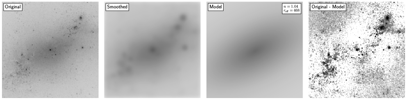
Figure 9: First panel: NGC 2337 ACS/WFC $F814W$ data product centred on the nuclear star cluster. The square region has side length $1000\text{\,}\mathrm{pixels}$ which corresponds to $\sim 2700\text{\,}\mathrm{parsec}$. Second panel: Smoothed version of the data shown in the first panel. We smooth the data using a two dimensional Gaussian kernel with a standard deviation of $\sigma=$21\text{\,}\mathrm{pixels}$$. Third panel: Fit to the smoothed data product shown in the second panel. We approximate the bar component with a Sérsic profile. The fit was performed with Imfit and the resulting Sérsic index $n$ and effective radius $r_{\mathrm{eff}}$ are indicated in the top right corner. Fourth panel: Residual map showing the difference between the science data (first panel) and the model of the bar (third panel).

A.2.2 Tests on AstroDrizzle & TinyTim using simulated data

Other systematic uncertainties could be induced by either AstroDrizzle or TinyTim. To test the chosen settings for both programs, we generated mock NSC data using the makeimage function of Imfit.

Simulated NSCs were created by convolving a Sérsic profile with a TinyTim-generated PSF. We added a flat background component whose values were randomly drawn from a Gaussian distribution. To test the influence of the settings of TinyTim, we fed this model and the PSF to Imfit and tried to recover the initial Sérsic indices and effective radii. To test the influence of AstroDrizzle, we took the science data of NGC 2337 and normalised it. We then superimposed the simulated NSC at the location of the NSCs on each exposure and performed AstroDrizzle. Afterwards, the simulated NSC was obtained from the output image of AstroDrizzle. The TinyTim-generated PSF was processed in the same way. The output data of AstroDrizzle were fed to Imfit where we tried to recover the initial Sérsic index and the effective radius. We repeated the fits for different Sérsic indices and effective radii starting from $(n=1,r_{\mathrm{eff}}=$10\text{\,}\mathrm{pixel}$)$ and going to $(n=3,r_{\mathrm{eff}}=$2\text{\,}\mathrm{pixel}$)$ in steps of $\delta n=1$ and $\delta r_{\mathrm{eff}}=$-1\text{\,}\mathrm{pixel}$$ (i.e. $27$ different settings). Two examples for the PSFs and the simulated NSCs are shown in the two left columns of Figure 10. The middle column shows two simulated NSCs convolved with the PSF and the right panels show the residual maps, including the recovered structural parameters and their uncertainties, as determined via $500$ bootstrap iterations.

If both the simulated NSC and the TinyTim-generated PSFs were not processed by AstroDrizzle, we recovered the initial structural parameter values for all combinations of $n$ and $r_{\mathrm{eff}}$ to high precision. Once we include AstroDrizzle for both the simulated NSC and the PSF, while using the same settings as for the science data, the structural parameters are recovered within the $1\sigma$ interval. The agreement with the initial parameter values is best for large effective radii and small Sérsic indices and becomes worse with more compact sources and steep profiles.

The recovered parameters became worse once we did not process the PSF with AstroDrizzle. In this case the PSFs were directly taken from TinyTim and rotated according to the orientation of the AstroDrizzle output. The uncertainty of the fit became larger and, in the case of a compact source with a steep inner slope, we were unable to recover the Sérsic index within the $1\sigma$ uncertainty distribution. Therefore, a significant systematic uncertainty is induced if the TinyTim-generated PSF is not processed in the same way as the science data.

We also tested settings related to TinyTim. We generated different PSFs assuming stellar templates ranging from F6V ($V-I=$0.55\text{\,}\mathrm{mag}$$) to K4V ($V-I=$1.13\text{\,}\mathrm{mag}$$) which covers the colour-range of typical NSCs (cf. Figure 11). Using these different PSFs on various science data yielded no significant differences in the resulting parameter values.

In addition, we evaluated whether the accuracy of placing PSFs onto normalised science data is an issue. More specifically, taking TinyTim-generated PSFs and superimposing them onto the normalised science data results in an accuracy of $\pm 1\text{\,}\mathrm{pixel}$. Therefore, we generated subsampled PSF (with subsampling factor ten), superimposed them on normalised single exposures (ACS/WFC data), processed the data with AstroDrizzle, resized the PSFs to the resolution of the science data, and applied the charge diffusion kernel. This approach should yield an accuracy of $\sim 0.1\text{\,}\mathrm{pixel}$. After fitting a few NSCs, we again found no significant differences and conclude that both the settings chosen in TinyTim and the uncertainty induced by placing PSFs onto normalised science exposures are insignificant.

Finally, we checked the modified AstroDrizzle parameters ‘pixel fraction’ and ‘resolution’. As briefly discussed in Section 3.1, we chose a value of $0.75$ for the pixel fraction and increased the final resolution according to the extent of the theoretical PSF for the ACS/WFC products. We conducted tests where we changed both the pixel fraction (between $0.5$ and $1.0$) and the final resolution [between $0.035\text{\,}\mathrm{arcsec}\text{\,}{\mathrm{pixel}}^{-1}$ and $0.05\text{\,}\mathrm{arcsec}\text{\,}{\mathrm{pixel}}^{-1}$ (original resolution)] but found no difference in the resulting parameter values. However, artifacts appeared in the weight maps of the data when choosing a low value for either the pixel fraction and resolution which indicate that AstroDrizzle cannot find input pixels from the individual exposures to generate a pixel value on the output grid. We verified that the different AstroDrizzle settings do not change the recovered structural parameter values of our mock data.

In conclusion, we cannot find significant systematic uncertainties induced by our approach. Note that systematic uncertainties can become significant once the PSF is not processed in the same way as the science data.

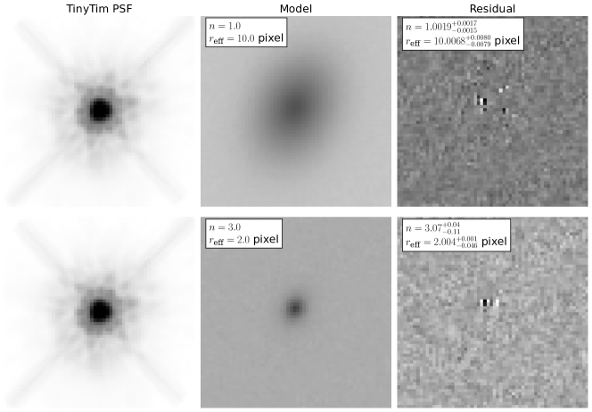
Figure 10: Left panels: TinyTim-generated PSFs using a G2V star as stellar template. The PSFs were superimposed on a normalised version of the science data of NGC 2337, processed with AstroDrizzle and extracted from the output image. Both PSFs are identical. Middle panels: 2D Sérsic profiles which have been convolved with the PSFs shown in the left panels. In addition, a flat background was added where the pixel values were randomly drawn from a Gaussian distribution. The top panel shows an extended profile whereas the bottom one is more compact and has a steeper centre, as indicated by the parameter values. The data processing with AstroDrizzle is equal to the approach used for the PSFs shown in the left panels. Right panels: Residual maps from fitting the Sérsic models (middle panels) using the PSFs shown in the left panels with Imfit. The structural parameters of the fit should equal the values used to generate the Sérsic models and are indicated in the central pictures.

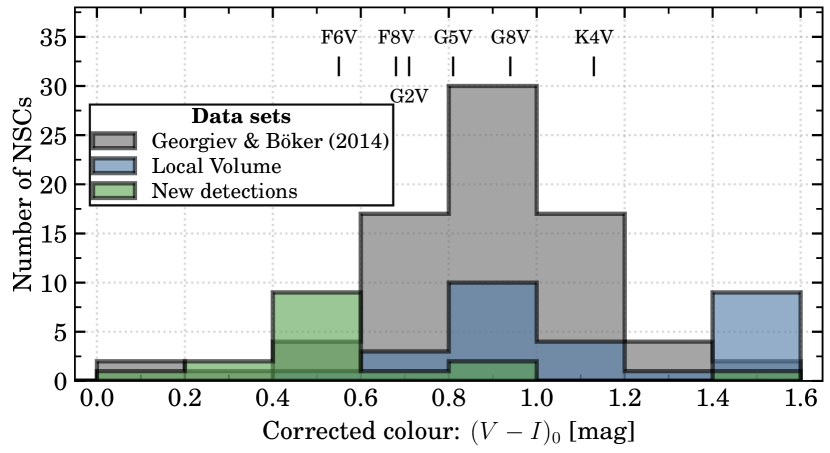
Figure 11: Nuclear star cluster $(V-I)_{0}$ colour. We compare our new detections (green) to other Local Volume data (blue) and the data set of Georgiev & Böker (2014) for nuclear star clusters in massive late-type field galaxies (gray). In addition, we highlight the colour of the different stellar templates tested for the synthetic point spread function. For the analysis in the main part of the paper, the template of a G2V star is used.

A.2.3 Fixation of Sérsic indices

As discussed in Section 3.3, the Sérsic index of a few NSCs diverges. To be able to approximate the effective radius of the NSCs, we fixed the index to a value of $n=2$. This value roughly equals the median value of the quality zero fits of the data set of Pechetti et al. (2020). We investigated the induced systematic uncertainty of this choice in Figure 12 where we show the Sérsic index versus effective radius. The plot shows three NSCs for which we repeated the fit with varying Sérsic indices. You can see that the effective radius is only slightly affected by the choice of Sérsic index between $n=0.5$ and $n=3.5$. At higher values of $n$ the effective radius increases and appears to diverge towards higher values. The only exception is M101-df4 for which $r_{\mathrm{eff}}$ appears to remain constant.

The figure shows that there exists a systematic uncertainty induced by fixing the Sérsic index to a value of $n=2$. Therefore, we determine the largest differences between effective radius between $n=0.5$ and $n=3$ and add this value in quadrature to the larger statistical uncertainty obtained from bootstrap iterations. If the ‘true’ Sérsic index is larger than $n=3$, our quoted effective radii become systematically too small, but as we show in Section 4.3, this issue does not affect our results.

Due to the choice of $n=2$, the apparent magnitudes of the NSCs are affected as well. In our tests the difference in magnitude is typically $\delta m\sim$0.1\text{\,}\mathrm{mag}$$ when setting $n=0.5$ and $n=3$. Therefore, for the cases where we set $n=2$ we add in quadrature to the statistical uncertainty the statistical uncertainty $0.1\text{\,}\mathrm{mag}$.

Finally, we tested the effect of fixing $n=2$ for the NSCs where the index did not diverge in the fits. Repeating the fits and using $500$ bootstrap iterations we find typical differences of $\delta r_{\mathrm{eff}}\lesssim$5\text{\,}\mathrm{\char 37\relax}$$ which is comparable to the statistical uncertainty

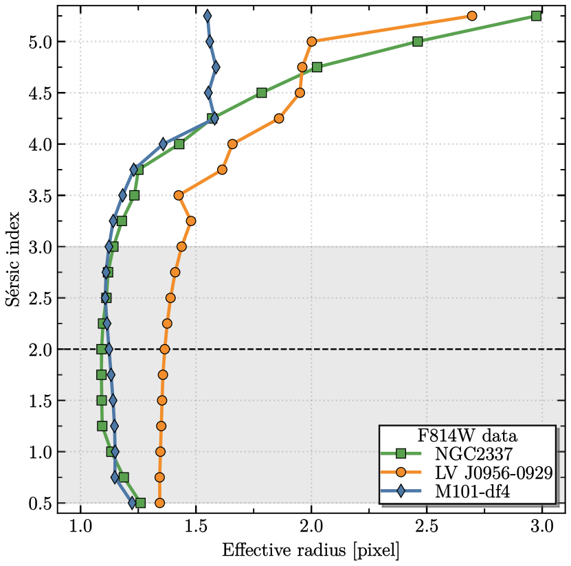
Figure 12: Fit results of three different nuclear star clusters (NGC 2337: green, LV J0956-0929: orange, M101-df4: blue) with fixed Sérsic indices. The dashed horizontal line shows the Sérsic value $n=2$ used to obtain an approximate value for the effective radii of the NSCs. The gray shaded area shows the range of Sérsic values which we consider to be reasonable given the indices of quality zero fits (i.e. ‘good’ fits) presented by Pechetti et al. (2020).

Appendix B Data tables

Here we present the data tables underlying this article. Appendix B gives an overview of the galaxies hosting the newly discovered NSCs and their available HST data. Galaxy properties are adapted from Hoyer et al. (2021) and raw images, containing exposure information, are taken from the HLA. Appendix B presents properties of the newly discovered NSCs. Appendix B gives the parameters of other NSCs in the Local Volume and in Appendix B we present the NSC stellar mass estimates of the data sample of Georgiev & Böker (2014).

Table 2: List of $21$ galaxies whose nuclear star clusters are new discoveries, sorted by descending galactic stellar mass. Galactic parameters (columns 2-5) are taken from Hoyer et al. (2021). The Proposal IDs and exposure times $t_{\mathrm{exp.}}$ are taken from the data products. For the ACS, we use an online calculator to obtain the zeropoint magnitudes: https://acszeropoints.stsci.edu/ For the WFPC2, we adopt the zeropoint magnitudes from the instrument’s manual (McMaster et al., 2008). For the WFC3, we use an online data base: https://www.stsci.edu/hst/instrumentation/wfc3/data-analysis/photometric-calibration/uvis-photometric-calibration.

Name	RA	DE	dm	$\log_{10}\,M_{\star}$	Instrument	Filter	Proposal ID	$m_{\mathrm{Inst.}}$	$t_{\mathrm{exp.}}$	pixel scale
	[deg]	[deg]	[mag]	[M⊙]				[VEGAmag]	[s]	[$\mathrm{arcsec}\text{\,}{\mathrm{pixel}}^{-1}$]
NGC 2337	105.55667	44.45694	$30.37\pm 0.49$	$8.97\pm 0.34$	ACS WFC	$F814W$	$13\,442$	$25.508$	$1000$	$0.0472$
						$F606W$	$13\,442$	$26.395$	$1000$	$0.0415$
LV J0956-0929	149.15667	-9.48639	$29.86\pm 0.11$	$8.29\pm 0.43$	ACS WFC	$F814W$	$12\,546$	$25.512$	$900$	$0.0472$
						$F606W$	$12\,546$	$26.398$	$900$	$0.0415$
[KK2000] 03	36.17792	-73.51278	$26.50\pm 0.09$	$8.16\pm 0.03$	ACS WFC	$F814W$	$13\,442$	$25.510$	$1200$	$0.0472$
						$F606W$	$13\,442$	$26.396$	$1200$	$0.0415$
UGC 09660	235.28875	44.69806	$30.16\pm 0.12$	$8.16\pm 0.32$	ACS WFC	$F814W$	$13\,442$	$25.510$	$1000$	$0.0472$
						$F606W$	$13\,442$	$26.396$	$1000$	$0.0415$
UGC 04998	141.30042	68.38306	$28.58\pm 0.21$	$8.13\pm 0.23$	WFPC2 PC	$F814W$	$8137$	$21.639$	$1500$	$0.05$
						$F555W$	$8137$	$22.545$	$1600$	$0.05$
UGC 01104	23.17625	18.31583	$29.39$	$8.00\pm 0.31$	WFPC2 WF	$F814W$	$9124$	$21.659$	$80$	$0.1$
						$F300W$	$9124$	$19.433$	$600$	$0.1$
LV J1205+2813	181.39250	28.23222	$31.45$	$7.92\pm 0.43$	ACS WFC	$F814W$	$13\,750$	$25.510$	$1218$	$0.0472$
						$F606W$	$13\,750$	$26.396$	$1000$	$0.0415$
DDO 133	188.22083	31.53917	$28.44\pm 0.05$	$7.80\pm 0.48$	WFPC2 WF	$F814W$	$10\,905$	$21.659$	$2200$	$0.1$
						$F606W$	$10\,905$	$22.896$	$2200$	$0.1$
UGC 07242	183.53083	66.09222	$28.68\pm 0.03$	$7.75\pm 0.43$	ACS WFC	$F814W$	$9771$	$25.525$	$900$	$0.0472$
						$F606W$	$9771$	$26.414$	$1200$	$0.0415$
PGC 154449	149.28708	-9.26333	$29.93$	$7.70\pm 0.39$	ACS WFC	$F814W$	$15\,922$	$25.507$	$760$	$0.0472$
						$F606W$	$15\,922$	$26.393$	$760$	$0.0415$
ESO 553-046	81.77375	-20.67806	$29.13\pm 0.02$	$7.68\pm 0.63$	ACS WFC	$F814W$	$12\,546$	$25.512$	$900$	$0.0472$
						$F606W$	$12\,546$	$26.395$	$900$	$0.0415$
DDO 084	160.67458	34.44889	$29.99$	$7.65\pm 0.35$	ACS WFC	$F814W$	$15\,922$	$25.507$	$760$	$0.0472$
						$F606W$	$15\,922$	$26.393$	$760$	$0.0415$
BTS 76	179.68375	27.58500	$30.50$	$7.53\pm 0.16$	ACS WFC	$F814W$	$14\,636$	$25.509$	$1030$	$0.0472$
						$F606W$	$14\,636$	$26.395$	$1030$	$0.0415$
M 101-df4	211.88917	54.71000	$32.16$	$7.29\pm 0.41$	ACS WFC	$F814W$	$13\,682$	$25.510$	$1150$	$0.0472$
						$F606W$	$13\,682$	$26.393$	$1150$	$0.0415$
NGC 5011C	198.29958	-43.26556	$27.86\pm 0.02$	$7.24\pm 0.53$	ACS WFC	$F814W$	$12\,546$	$25.512$	$900$	$0.0472$
						$F606W$	$12\,546$	$26.398$	$900$	$0.0415$
LeG 09	160.64417	12.15056	$30.04\pm 0.07$	$7.08\pm 0.43$	ACS WFC	$F814W$	$14\,644$	$25.509$	$1096$	$0.0472$
						$F606W$	$14\,644$	$26.395$	$1026$	$0.0415$
[KK2000] 53	197.80917	-38.90611	$27.33\pm 0.07$	$6.85\pm 0.44$	ACS WFC	$F814W$	$13\,442$	$25.510$	$1000$	$0.0472$
						$F606W$	$13\,442$	$26.397$	$1000$	$0.0415$
KK 96	162.61292	12.36083	$30.00\pm 0.04$	$6.68\pm 0.43$	ACS WFC	$F814W$	$14\,644$	$25.509$	$1096$	$0.0472$
						$F606W$	$14\,644$	$26.395$	$1026$	$0.0415$
LV J1217+4703	184.29208	47.06361	$30.70\pm 0.22$	$6.58\pm 0.50$	ACS WFC	$F814W$	$14\,644$	$25.509$	$1164$	$0.0472$
						$F606W$	$14\,644$	$26.395$	$1094$	$0.0415$
PGC 4310323	181.37917	31.07611	$29.04$	$6.55\pm 0.43$	ACS WFC	$F814W$	$15\,922$	$25.507$	$760$	$0.0472$
						$F606W$	$15\,922$	$26.393$	$760$	$0.0415$
dw 1335-29	203.94167	-29.70667	$28.50\pm 0.21$	$6.46\pm 0.43$	ACS SBC	$F150LP$	$10\,608$	$20.747$	$5416$	$0.03$

Table 3: Structural and photometric parameters of the $21$ newly discovered nuclear star clusters in the Local Volume. All values are the median of the parameter distribution after $500$ bootstrapping iterations. The uncertainties give the $1\sigma$ interval.

• The structural parameters in this filter were fixed to the values determined via bootstrapping in the other available filter.

• The Sérsic index is fixed to $n=2$ to determine an effective radius. All other parameters are unrestricted (cf. Table 1).

• The NSC mass estimate is unreliable as the mass-to-light ratio is too large ($M_{\star}/L_{I}\gtrsim 4\mathrm{M}_{\odot}/\mathrm{L}_{\odot}$).

• No fit was possible.

Table 4: List of compiled properties of known nuclear star clusters (NSCs) in the Local Volume. Only NSCs with available structural parameters are included.

• References: (1) Baldassare et al. (2014); (2) Bellazzini et al. (2020); (3) Calzetti et al. (2015); (4) Carson et al. (2015); (5) Crnojević et al. (2016); (6) Georgiev et al. (2009); (7) Georgiev & Böker (2014); (8) Graham & Spitler (2009); (9) Kormendy & Bender (1999); (10) Kormendy et al. (2010); (11) Nguyen et al. (2017); (12) Nguyen et al. (2018); (13) Pechetti et al. (2020); (14) Schödel et al. (2014); (15) Seth et al. (2006)

Table 5: List of $V$- and $I$-band apparent magnitudes and stellar mass estimates of nuclear star clusters (NSCs) in the galaxy sample of Georgiev & Böker (2014). NSC structural parameters are presented in the data tables of Georgiev & Böker (2014).

References

- Agarwal & Milosavljević (2011) Agarwal M., Milosavljević M., 2011, ApJ, 729, 35
- Antonini (2013) Antonini F., 2013, ApJ, 763, 62
- Antonini et al. (2012) Antonini F., Capuzzo-Dolcetta R., Mastrobuono-Battisti A., Merritt D., 2012, ApJ, 750, 111
- Antonini et al. (2015) Antonini F., Barausse E., Silk J., 2015, ApJ, 812, 72
- Baldassare et al. (2014) Baldassare V. F., Gallo E., Miller B. P., Plotkin R. M., Treu T., Valluri M., Woo J.-H., 2014, ApJ, 791, 133
- Bastian (2008) Bastian N., 2008, MNRAS, 390, 759
- Baumgardt & Hilker (2018) Baumgardt H., Hilker M., 2018, MNRAS, 478, 1520
- Bellazzini et al. (2020) Bellazzini M., Annibali F., Tosi M., Mucciarelli A., Cignoni M., Beccari G., Nipoti C., Pascale R., 2020, A&A, 634, A124
- Bender et al. (2005) Bender R., et al., 2005, ApJ, 631, 280
- Boggs & Rogers (1990) Boggs P. T., Rogers J. E., 1990, in Statistical analysis of measurement error models and applications: proceedings of the AMS-IMS-SIAM joint summer research conference held June 10-16 1989. Contemporary Mathematics, p. 186, https://archive.org/details/orthogonaldistan8941bogg
- Böker et al. (1999) Böker T., et al., 1999, ApJS, 124, 95
- Böker et al. (2002) Böker T., Laine S., van der Marel R. P., Sarzi M., Rix H.-W., Ho L. C., Shields J. C., 2002, AJ, 123, 1389
- Boulade et al. (2003) Boulade O., et al., 2003, in Iye M., Moorwood A. F. M., eds, Vol. 4841, Instrument Design and Performance for Optical/Infrared Ground-based Telescopes. SPIE, pp 72–81, https://ui.adsabs.harvard.edu/abs/2003SPIE.4841...72B/abstract
- Calzetti et al. (2015) Calzetti D., et al., 2015, ApJ, 811, 75
- Carlsten et al. (2020) Carlsten S. G., Greco J. P., Beaton R. L., Greene J. E., 2020, ApJ, 891, 144
- Carlsten et al. (2022) Carlsten S. G., Greene J. E., Beaton R. L., Greco J. P., 2022, ApJ, 927, 44
- Carollo et al. (1998) Carollo C. M., Stiavelli M., Mack J., 1998, AJ, 116, 68
- Carson et al. (2015) Carson D. J., Barth A. J., Seth A. C., den Brok M., Cappellari M., Greene J. E., Ho L. C., Neumayer N., 2015, AJ, 149, 149
- Côté et al. (2006) Côté P., et al., 2006, ApJS, 165, 57
- Crnojević et al. (2016) Crnojević D., Sand D. J., Zaritsky D., Spekkens K., Willman B., Hargis J. R., 2016, ApJL, 824, L14
- Den Brok et al. (2014) Den Brok M., et al., 2014, MNRAS, 445, 2385
- Dehnen (2005) Dehnen W., 2005, MNRAS, 360, 892
- Dolphin (2009) Dolphin A. E., 2009, PASP, 121, 655
- Erwin (2015) Erwin P., 2015, ApJ, 799, 226
- Fahrion et al. (2020) Fahrion K., et al., 2020, A&A, 634, A53
- Fahrion et al. (2021) Fahrion K., et al., 2021, A&A, 650, A137
- Fahrion et al. (2022a) Fahrion K., et al., 2022a,
- Fahrion et al. (2022b) Fahrion K., Leaman R., Lyubenova M., van de Ven G., 2022b, A&A, 658, A172
- Feldmeier-Krause et al. (2015) Feldmeier-Krause A., et al., 2015, A&A, 584, A2
- Feldmeier-Krause et al. (2017) Feldmeier-Krause A., Kerzendorf W., Neumayer N., Schödel R., Nogueras-Lara F., Do T., de Zeeuw P. T., Kuntschner H., 2017, MNRAS, 464, 194
- Ferrarese et al. (2012) Ferrarese L., et al., 2012, ApJS, 200, 4
- Ferrarese et al. (2020) Ferrarese L., et al., 2020, ApJ, 890, 128
- Fitzpatrick (1999) Fitzpatrick E. L., 1999, PASP, 111, 63
- Fruchter & Hook (1997) Fruchter A. S., Hook R. N., 1997, in Tescher A. G., ed., Vol. 3164, Applications of Digital Image Processing XX. pp 120–125 (arXiv:9708242), doi:10.1117/12.292751, https://ui.adsabs.harvard.edu/abs/1997SPIE.3164..120F
- Georgiev & Böker (2014) Georgiev I. Y., Böker T., 2014, MNRAS, 441, 3570
- Georgiev et al. (2009) Georgiev I. Y., Puzia T. H., Hilker M., Goudfrooij P., 2009, MNRAS, 392, 879
- Georgiev et al. (2016) Georgiev I. Y., Böker T., Leigh N., Lützgendorf N., Neumayer N., 2016, MNRAS, 457, 2122
- Georgiev et al. (2019) Georgiev I. Y., et al., 2019, MNRAS, 484, 3356
- Gonzaga et al. (2012) Gonzaga S., Hack W., Fruchter A., Mack J., 2012, The DrizzlePac Handbook. https://ui.adsabs.harvard.edu/abs/2012drzp.book.....G
- Graham & Driver (2005) Graham A. W., Driver S. P., 2005, PASA, 22, 118
- Graham & Spitler (2009) Graham A. W., Spitler L. R., 2009, MNRAS, 397, 2148
- Green (2018) Green G. M., 2018, The Journal of Open Source Software, 3, 695
- Habas et al. (2020) Habas R., et al., 2020, MNRAS, 491, 1901
- Harris (1996) Harris W. E., 1996, AJ, 112, 1487
- Harris et al. (2020) Harris C. R., et al., 2020, Nature, 585, 357
- Hartmann et al. (2011) Hartmann M., Debattista V. P., Seth A. C., Cappellari M., Quinn T. R., 2011, MNRAS, 418, 2697
- Hoyer et al. (2021) Hoyer N., Neumayer N., Georgiev I. Y., Seth A. C., Greene J. E., 2021, MNRAS, 507, 3246
- Hunter (2007) Hunter J. D., 2007, Computing in Science & Engineering, 9, 90
- Kacharov et al. (2018) Kacharov N., Neumayer N., Seth A. C., Cappellari M., McDermid R., Walcher C. J., Böker T., 2018, MNRAS, 480, 1973
- Karachentsev et al. (2013) Karachentsev I. D., Makarov D. I., Kaisina E. I., 2013, AJ, 145, 101
- King (1962) King I., 1962, AJ, 67, 471
- King (1966) King I. R., 1966, AJ, 71, 64
- Kormendy & Bender (1999) Kormendy J., Bender R., 1999, ApJ, 522, 772
- Kormendy & Ho (2013) Kormendy J., Ho L. C., 2013, ARAA, 51, 511
- Kormendy et al. (2010) Kormendy J., Drory N., Bender R., Cornell M. E., 2010, ApJ, 723, 54
- Krist (1993) Krist J., 1993, in Hanisch R. J., Brissenden R. J. V., Barnes J., eds, Vol. 52, Astronomical Data Analysis Software and Systems II. p. 536, https://ui.adsabs.harvard.edu/abs/1993ASPC...52..536K
- Krist (1995) Krist J., 1995, in Shaw R. A., Payne H. E., Hayes J. J. E., eds, Vol. 77, Astronomical Data Analysis Software and Systems IV. p. 349, https://adass.org/adass/proceedings/adass94/kristj.html
- Kruijssen & Cooper (2012) Kruijssen J. M. D., Cooper A. P., 2012, MNRAS, 420, 340
- Leaman & van de Ven (2022) Leaman R., van de Ven G., 2022, MNRAS, 516, 4691
- Leaman et al. (2020) Leaman R., et al., 2020, MNRAS, 492, 5102
- Lu et al. (2009) Lu J. R., Ghez A. M., Hornstein S. D., Morris M. R., Becklin E. E., Matthews K., 2009, ApJ, 690, 1463
- Makarov et al. (2014) Makarov D., Prugniel P., Terekhova N., Courtois H., Vauglin I., 2014, A&A, 570, A13
- McLaughlin & van der Marel (2005) McLaughlin D. E., van der Marel R. P., 2005, ApJS, 161, 304
- McMaster et al. (2008) McMaster M., et al., 2008, Wide Field and Planetary Camera 2 Instrument Handbook v. 10.0. Space Telescope Science Institude (STScI), Balitmore, USA
- Miller & Lotz (2007) Miller B. W., Lotz J. M., 2007, ApJ, 670, 1074
- Milosavljević (2004) Milosavljević M., 2004, ApJL, 605, L13
- Muñoz et al. (2015) Muñoz R. P., et al., 2015, ApJL, 813, L15
- Neumayer et al. (2011) Neumayer N., Walcher C. J., Andersen D., Sánchez S. F., Böker T., Rix H.-W., 2011, MNRAS, 413, 1875
- Neumayer et al. (2020) Neumayer N., Seth A. C., Böker T., 2020, AAPR, 28, 75
- Nguyen et al. (2017) Nguyen D. D., et al., 2017, ApJ, 836, 237
- Nguyen et al. (2018) Nguyen D. D., et al., 2018, ApJ, 858, 118
- Nguyen et al. (2019) Nguyen D. D., et al., 2019, ApJ, 872, 104
- Norris et al. (2014) Norris M. A., et al., 2014, MNRAS, 443, 1151
- Ordenes-Briceño et al. (2018) Ordenes-Briceño Y., et al., 2018, ApJ, 860, 4
- Parmentier & Gilmore (2007) Parmentier G., Gilmore G., 2007, MNRAS, 377, 352
- Pechetti et al. (2020) Pechetti R., Seth A. C., Neumayer N., Georgiev I. Y., Kacharov N., den Brok M., 2020, ApJ, 900, 32
- Peng et al. (2008) Peng E. W., et al., 2008, ApJ, 681, 197
- Poulain et al. (2021) Poulain M., et al., 2021, MNRAS, 506, 5494
- Roediger & Courteau (2015) Roediger J. C., Courteau S., 2015, MNRAS, 452, 3209
- Ryon et al. (2019) Ryon J. E., et al., 2019, Advanced Camera for Surveys Instrument Handbook for Cycle 27. Space Telescope Science Institude (STScI), Balitmore, USA
- Sánchez-Janssen et al. (2019) Sánchez-Janssen R., et al., 2019, ApJ, 878, 18
- Schlafly & Finkbeiner (2011) Schlafly E. F., Finkbeiner D. P., 2011, ApJ, 737, 103
- Schlegel et al. (1998) Schlegel D. J., Finkbeiner D. P., Davis M., 1998, ApJ, 500, 525
- Schödel et al. (2014) Schödel R., Feldmeier A., Kunneriath D., Stolovy S., Neumayer N., Amaro-Seoane P., Nishiyama S., 2014, A&A, 566, A47
- Sérsic (1968) Sérsic J. L., 1968, Atlas de Galaxias Australes. Universidad Nacional de Cordoba, https://ui.adsabs.harvard.edu/abs/1968adga.book.....S
- Seth et al. (2006) Seth A. C., Dalcanton J. J., Hodge P. W., Debattista V. P., 2006, AJ, 132, 2539
- Sirianni et al. (2005) Sirianni M., et al., 2005, PASP, 117, 1049
- Smith et al. (2016) Smith R., Choi H., Lee J., Rhee J., Sanchez-Janssen R., Yi S. K., 2016, ApJ, 833, 109
- Spengler et al. (2017) Spengler C., et al., 2017, ApJ, 849, 55
- Stahler (2018) Stahler S., 2018, The Birth of Star Clusters. Astrophysics and Space Science Library, Springer Cham, https://link.springer.com/book/10.1007/978-3-319-22801-3
- Storn & Price (1997) Storn R., Price K., 1997, Journal of Global Optimization, 11, 341
- Su et al. (2021) Su A. H., et al., 2021, A&A, 647, A100
- The Astropy Collaboration et al. (2013) The Astropy Collaboration et al., 2013, A&A, 558, A33
- The Astropy Collaboration et al. (2018) The Astropy Collaboration et al., 2018, ApJ, 156, 123
- Tremaine et al. (1975) Tremaine S. D., Ostriker J. P., Spitzer L., 1975, ApJ, 196, 407
- Turner et al. (2012) Turner M. L., Côté P., Ferrarese L., Jordán A., Blakeslee J. P., Mei S., Peng E. W., West M. J., 2012, ApJS, 203, 5
- Venhola et al. (2018) Venhola A., et al., 2018, A&A, 620, A165
- Virtanen et al. (2020) Virtanen P., et al., 2020, Nature Methods, 17, 261
- Walcher et al. (2005) Walcher C. J., et al., 2005, ApJ, 618, 237
- Walcher et al. (2006) Walcher C.-J., Böker T., Charlot S., Ho L. C., Rix H.-W., Rossa J., Shields J. C., van der Marel R. P., 2006, ApJ, 649, 692
- Wegner et al. (2000) Wegner M., et al., 2000, A&ASS, 143, A9
- Zanatta et al. (2021) Zanatta E., Sánchez-Janssen R., Chies-Santos A. L., de Souza R. S., Blakeslee J. P., 2021, MNRAS, 508, 986