Abstract

Many dynamical systems in the real world are naturally described by latent states with intrinsic ordering, such as “ally”, “neutral”, and “enemy” relationships in international relations. These latent states manifest through countries’ cooperative versus conflictual interactions over time. State-space models (SSMs) explicitly relate the dynamics of observed measurements to transitions in latent states. For discrete data, SSMs commonly do so through a state-to-action emission matrix and a state-to-state transition matrix. This paper introduces the Ordered Matrix Dirichlet (OMD) as a prior distribution over ordered stochastic matrices wherein the discrete distribution in the $k^{\textrm{th}}$ row is stochastically dominated by the $(k\!+\!1)^{\textrm{th}}$, such that probability mass is shifted to the right when moving down rows. We illustrate the OMD prior within two SSMs: a hidden Markov model, and a novel dynamic Poisson Tucker decomposition model tailored to international relations data. We find that models built on the OMD recover interpretable ordered latent structure without forfeiting predictive performance. We suggest future applications to other domains where models with stochastic matrices are popular (e.g., topic modeling), and publish user-friendly code.

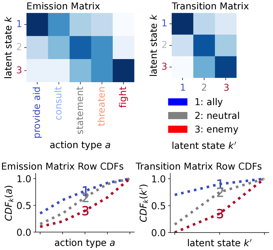
Figure 1: Action types in international relations data are ordered along a cooperation-to-conflict axis. Our model infers latent states with an ordering that reflects the ordering in observed actions. Emission matrix: more conflictual actions (indexed by higher $a$), are generated by more conflictual latent states (higher $k$). Transition matrix: latent states transition to neighboring ones. CDFs: The Ordered Matrix Dirichlet enforces that the CDF of the $k^{\textrm{th}}$ discrete distribution is always greater than the $(k\!+\!1)^{\textrm{th}}$, so that probability mass in the stochastic matrix shifts right when moving down rows.

1 INTRODUCTION

In many modeling settings and application domains, some aspect of the observation space has intrinsic ordering. For example, in international relations, observed interactions between countries can be ordered on a conflict-to-cooperation axis, ranging from “provide aid” to “fight” (Goldstein,, 1992; Schrodt,, 2008). This ordering should ideally be reflected in any state space used to summarize or describe observed interactions. For example, more conflictual actions like “fight” or “threaten” might be more likely between countries in an “enemy” state than those in an “ally”state (Schrodt,, 2006). In this example, the latent states represent relationship statuses between countries, ordered from “ally” to “enemy”, and reflect the conflict-to-cooperation ordering of the observed actions. We might expect states to transition to other states over time in a way that also reflects their intrinsic ordering. Allies rarely become enemies from one moment to the next, but rather (de-)escalate gradually, passing first through intermediate states (Davis and Stan, 1984a, ).

State-space models (SSMs) are statistical models that explicitly relate time-varying measurements to latent states, such that patterns and trends in the observed space are attributable to transitions between states over time. For discrete data, the canonical form of such models is based on two stochastic matrices: the emission matrix, which describes how latent states generate observations, and the transition matrix, which describes how states transition to other states over time. This general formulation does not intrinsically promote any ordering of the latent states, whose indices are arbitrary and subject to “label switching” (Richardson and Green,, 1997; Stephens,, 2000).

To promote some sense of ordering in the state space, researchers sometimes constrain the transition matrix to take only banded or “left-right-left” forms (Schrodt,, 2006; Netzer et al.,, 2008; Randahl and Vegelius,, 2022), whereby states only transition to adjacent states. This constraint substantially restricts the expressiveness of the model while still not ensuring a well-defined ordering of the latent states that reflects the ordering in the observation space.

This paper introduces a novel prior distribution over stochastic matrices, the Ordered Matrix Dirichlet (OMD), and demonstrates it as a key ingredient in SSMs with well-ordered state spaces. An OMD random variable is a stochastic matrix whose rows are discrete distributions that sum to 1, and whose $k^{\textrm{th}}$ row is stochastically dominated by the $(k\!+\!1)^{\textrm{th}}$, so that probability mass shifts to the right when moving down the matrix (Fig. 1). We define the OMD distribution implicitly via a stick-breaking construction that ensures the desired ordering property by sorting Beta-distributed auxiliary variables. As we show, when the OMD is selected as a prior over both emission and transition matrices in an SSM, the inferred latent states have an intrinsic ordering that reflects ordering in the observation space.

To demonstrate and evaluate the OMD as a prior, we construct and apply two different SSMs—(1) a simple hidden Markov model (HMM) that we apply to synthetic data where the ground-truth latent structure is known, and (2) a novel dynamic version of Bayesian Poisson Tucker decomposition (Schein et al., 2016b, ), which we apply to international relations data of country-to-country interactions.

We compare each of these models to a baseline that differs only in its prior over the transition and emission matrices—instead of the OMD, it makes the standard assumption of rows being independently Dirichlet-distributed, which we term the Standard Matrix Dirichlet (SMD). We find that the models based on the OMD are more readily interpretable than those based on the SMD while still performing comparably and sometimes better in forecasting and imputation tasks. In synthetic experiments, the OMD model is much more effective at recovering ground-truth latent structure, while on international relations data, the OMD model exhibits superior forecasting performance over both the SMD model and an additional baseline we introduce that constrains the transition matrix to be banded.

After setting up notation and providing background on SSMs in § 2, we formally introduce the OMD in § 3 and motivate it as a prior within SSMs. In § 4 we discuss posterior inference for OMD models using Pyro (Bingham et al.,, 2018). We then provide results from a suite of synthetic data experiments in § 5, and present a case study on international relations data in § 6. Finally, we discuss broader connections in § 7, and summarize our conclusions in § 8.

2 STATE-SPACE MODELS

State-space models (SSMs) describe the evolution of time-indexed measurements $\boldsymbol{y}^{(t)}$ in terms of corresponding latent states $\boldsymbol{\lambda}^{(t)}$ (Kalman,, 1960). SSMs assume that patterns and trends in the observed measurements, typically only noisily realized, are attributable to transitions between latent states.

Basic Form

This paper considers a subset of SSMs frequently used to model discrete or non-negative data. Consider a non-negative vector-valued measurement $\boldsymbol{y}^{(t)}\in\mathbb{R}_{+}^{A}$ at discrete time step $t$. Using the international relations example in the introduction, $\boldsymbol{y}^{(t)}$ might measure the counts of $A$ different action types taken between some pair of countries during time step $t$. We use $a\in[A]$ to index into this vector, so that $y^{(t)}_{a}$ is an entry, and refer to $a$ as an action or action type throughout.

The SSMs we consider connect observed measurements to vector-valued, non-negative latent states $\boldsymbol{\lambda}^{(t)}\in\mathbb{R}_{+}^{K}$ under the following assumption:

$$\mathbb{E}[y^{(t)}_{a}] \propto\sum_{k=1}^{K}\lambda^{(t)}_{k}\underbrace{\phi_{ka}}_{\text{emission}}$$ (1)

where $\phi_{ka}\in[0,1]$ is an entry in the discrete distribution $\boldsymbol{\phi}_{k}$ which sums to one over actions $\sum_{a=1}^{A}\phi_{ka}\!=\!1$ and is itself the $k^{\textrm{th}}$ row of the state-to-action emission matrix $\Phi$.

The states then evolve over time under the assumption

$${\mathbb{E}}[\lambda^{(t)}_{k}] \propto\sum_{k^{\prime}=1}^{K}\lambda^{(t\!-\!1)}_{k^{\prime}}\underbrace{\pi_{k^{\prime}k}}_{\text{transition}}$$ (2)

where $\pi_{k^{\prime}k}\in[0,1]$ is an entry in the discrete distribution $\boldsymbol{\pi}_{k^{\prime}}$ which is itself the $(k^{\prime})^{\textrm{th}}$ row of the state-to-state transition matrix $\Pi\in[0,1]^{K\times K}$.

Many SSMs follow this basic form in  1 and 2, such as hidden Markov models (HMMs), discrete dynamical systems (Schein et al., 2016a, ), or more complex SSMs as presented in § 6.2. The key feature of these models is that they involve an emission $\Phi$ and transition matrix $\Pi$ which are both (row-)stochastic matrices.

What is a “State”?

There are differences in the SSM literature on whether the “state” at time step $t$ is the vector $\boldsymbol{\lambda}^{(t)}$, or whether each element $\lambda^{(t)}_{k}$ of the vector describes the relevance of one of $k\in[K]$ “states”. These two interpretations coincide when $\boldsymbol{\lambda}^{(t)}$ is a one-hot vector, placing non-zero mass on only one element, as in HMMs. However, these interpretations diverge in more general settings. We adopt both senses of the word “state” in this paper, referring to $\boldsymbol{\lambda}^{(t)}$ as the complex “state” of the overall system at $t$ but also understanding it as a mixture over $K$ simple “states”.

Dirichlet Priors

Researchers often place prior distributions over model parameters either as a way to encode structural assumptions about the state space or to fit models using Bayesian inference (or both). The conventional prior for row-stochastic matrices assumes that rows are independently Dirichlet distributed, what we will refer to as the Standard Matrix Dirichlet (SMD). A draw $\boldsymbol{\phi}\sim\textrm{Dir}(\boldsymbol{\alpha})$ from a Dirichlet distribution with concentration parameter $\boldsymbol{\alpha}\in\mathbb{R}_{+}^{A}$ is a discrete distribution over $A$ categories, $\sum_{a=1}^{A}\phi_{a}\!=\!1$.

Banded Constraints

One commonly-used constraint is that the transition matrix is banded along its diagonal, such that $\pi_{k^{\prime}k}=0$ if $|k-k^{\prime}|>b$ for some bandwidth $b$ (often set to 1); see the middle plot of Fig. 2. This constraint encodes the assumption that states only excite or transition to nearby states at subsequent time steps. Such an assumption is motivated, for example, when the desired state space represents ordered stages of escalation in international conflict (Schrodt,, 2006; Randahl and Vegelius,, 2022). For purposes of comparison, we introduce a prior distribution called the Banded Matrix Dirichlet (BMD) that enforces this constraint (§ B.2).

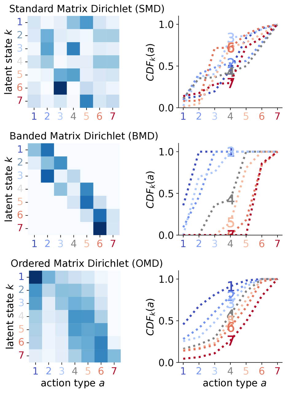
Figure 2: Stochastic matrices sampled from the Standard Matrix Dirichlet (SMD), Banded Matrix Dirichlet (BMD) and Ordered Matrix Dirichlet (OMD). Neither the SMD nor the BMD adhere to the stochastic dominance property in Eq. 3, as evidenced by overlapping CDFs.

3 THE ORDERED MATRIX DIRICHLET

Many dynamical systems in the real world are naturally described by latent states with intrinsic ordering, such as in international relations, where the relationship status of two countries might escalate from “ally” to “enemy” only gradually, first passing through intermediate states like “neutral”. In addition to constraining how states transition over time, this ordering may further reflect ordering in the observed actions between countries, with countries in more conflictual latent states (e.g., “enemy”) taking more conflictual actions towards each other (e.g., “fight”), and countries in more cooperative states (e.g., “ally”) taking more cooperative actions (e.g., “provide aid”).

The state space in the basic model formulation given in Eq. 1 and Eq. 2 is not intrinsically ordered. Specifically, the row indices $k\in[K]$ of the emission and transition matrices are arbitrary and bear no intrinsic information. As mentioned in the previous section, constraining the transition matrix to be banded does impart some information to the index $k$. However, its interpretation is circular: $k$ is some state that transitions to other states $\{k^{\prime}:|k-k^{\prime}|\leq b\}$, whose interpretation is similarly defined with respect to $k$. Moreover, while banding the transition matrix promotes some ordering of latent states, it does not promote one that necessarily reflects the ordering in observed actions.

To overcome these limitations, this section introduces a novel prior over the transition and emission matrices that ensures an intrinsically well-ordered state space, one that both reflects the ordering in observed actions and the ordering in latent state transitions. We first operationalize our notion of ordering in terms of stochastic dominance, and then construct a probability distribution with support over the subset of stochastic matrices that obey this notion.

3.1 Ordering by Stochastic Dominance

Considering first the emission matrix, each row $\boldsymbol{\phi}_{k}$ represents a discrete distribution over ordinal actions types. Intuitively, we might say the rows are well-ordered if probability mass shifts to the right when moving down rows, or equivalently, when the $k^{\textrm{th}}$ distribution places more weight on earlier action types than the $(k\!+\!1)^{\textrm{th}}$. This intuition is formalized by the notion of stochastic dominance (Davidson,, 2017). Define the cumulative distribution function (CDF) for the $k^{\textrm{th}}$ discrete distribution to be $\mathrm{CDF}_{k}(a)\triangleq\sum_{a^{\prime}=1}^{a}\phi_{ka^{\prime}}$. Then, the $k^{\textrm{th}}$ distribution is stochastically dominated by the $(k\!+\!1)^{\textrm{th}}$ if

$$\mathrm{CDF}_{k}(a)\geq\mathrm{CDF}_{k\!+\!1}(a)\,\,\textrm{ for all }a$$ (3)

We refer to a stochastic matrix as well-ordered if Eq. 3 holds for all rows $k$. For the $K\times A$ emission matrix, this means higher rows place more mass on earlier actions types. For the $K\times K$ transition matrix, this notion encapsulates many but not all banded structures (see Fig. 2), while further allowing for much more flexible “down-and-right” transition shapes (see Fig. 4).

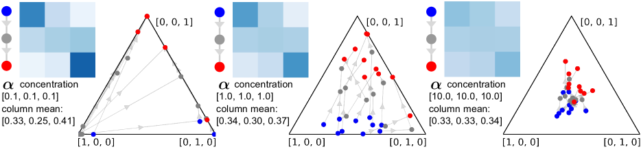
Figure 3: Heatmaps: Averages of 10 samples from the Ordered Matrix Dirichlet with varying concentration ${\boldsymbol{\alpha}}\in\mathbb{R}_{+}^{A}$. “Column mean” refers to $\overline{\phi_{a}}=\frac{1}{K}\sum_{k=1}^{K}{\boldsymbol{\phi}}_{ka}$ and shows that probability mass is asymmetric to the right. Simplex plots: Each point is a discrete distribution over $A=3$ classes. The $K=3$ points ( , , ) connected by a line represent one sample from the OMD. We observe ordered transitions from the lower left $[1,0,0]$ to the top $[0,0,1]$ corner of the simplex. In Fig. 12 in App. C, we present unordered sample trajectories from the SMD in comparison.

3.2 Ordered Matrix Dirichlet (OMD) Distribution

We now introduce a new probability distribution that has support over only the matrices described above. The OMD distribution is defined by two parameters, concentration ${\boldsymbol{\alpha}}\in\mathbb{R}_{+}^{A}$ and height $K$. An OMD random variable $\Phi\sim\textrm{\text{OMD}}(K,{\boldsymbol{\alpha}})$ is a $K\times A$ matrix that is row-stochastic and well-ordered, as shown in Proposition 3.1.

We define the OMD distribution implicitly via Algorithm 1, which generates OMD variates. This algorithm builds on the stick-breaking construction of the standard Dirichlet distribution (Gelman et al.,, 2013, p. 583). A Dirichlet random variable $\phi\sim\textrm{Dir}(\boldsymbol{\alpha})$ can be generated iteratively, one entry at a time, via Beta auxiliary variables. First, draw $\phi_{1}\sim\textrm{Beta}(\alpha_{1},\sum_{a>1}\alpha_{a})$. Then for $a=2,\dots,A\!-\!1$ draw $\beta_{a}\sim\textrm{Beta}(\alpha_{a},\sum_{a^{\prime}>a}\alpha_{a^{\prime}})$ and set $\phi_{a}\leftarrow\beta_{a}\,(1-\sum_{a^{\prime}<a}\phi_{a^{\prime}})$. Finally, set $\phi_{A}\leftarrow 1-\sum_{a^{\prime}<A}\phi_{a^{\prime}}$. Intuitively, this construction iteratively “breaks” off some amount of remaining probability mass (the “stick”), where the Beta variables determine the size of the breaks.

Algorithm 1 iteratively constructs $K$ discrete distributions over $A$ categories using the same basic idea. For each category $a$ in succession, it samples $K$ Beta variables (lines 3 and 8) to determine the size of the “breaks” in the $K$ “sticks”. However, it further sorts the Beta variables (lines 5 and 10), so that the largest “break” of the remaining “stick” is always taken by the first “stick” ($k=1$), the second largest is always taken by the second “stick” ($k=2$), and so on. In so doing, it generates a well-ordered stochastic matrix, as stated below.

Proposition 3.1 (OMD random variables are well-ordered).

The OMD has support over only row-stochastic matrices that obey the ordering property given beneath Eq. 3, such that for any two rows $k<k^{\prime}$ and any $a$

$$\sum_{a^{\prime}\leq a}\phi_{ka^{\prime}}\geq\sum_{a^{\prime}\leq a}\phi_{k^{\prime}a^{\prime}}$$ (4)

Proof: See § B.1.

Lack of Analytic Form

We define the OMD implicitly by construction and do not (yet) know any analytic form for its probability density function (PDF), which involves integrating over products of Beta order statistics. We leave further investigation into the OMD’s PDF, moments, and other analytic properties for the future. As we show in the next section though, its lack of analytic form does not hamper posterior inference with modern probabilistic programming.

What is “Dirichlet” about the OMD?

The OMD’s name reflects its definition as a minimal modification to the stick-breaking construction of the Standard Matrix Dirichlet—if we remove the blue lines (5 and 10), then Algorithm 1 corresponds exactly to the SMD, which simply generates $K$ independent Dirichlet variates (with no ordering). The name reflects this alone—it is not the case (to our knowledge) that the $K$ discrete distributions, which are dependent under the OMD via the sort operation, are marginally or conditionally Dirichlet distributed.

Algorithm 1 Ordered Matrix Dirichlet

1:Input: height $K$, concentration ${\boldsymbol{\alpha}}\in\mathbb{R}_{+}^{A}$

2:for $k=1,\,\dots\,,K$ do

3:     $\tilde{{\boldsymbol{\phi}}}_{k1}\sim\textrm{Beta}\left(\alpha_{1},\sum_{a=2}^{A}\alpha_{a}\right)$

4:end for

5:$(\phi_{11},\dots,\phi_{K1})\leftarrow\textsc{Sort}\Big{(}(\tilde{\phi}_{11},\dots,\tilde{\phi}_{K1})\Big{)}$

6:for $a=2,\,\dots\,,\,A-1$ do

7:     for $k=1,\,\dots\,,K$ do

8:         $\tilde{\beta}_{ka}\sim\textrm{Beta}\left(\alpha_{a},\sum_{a^{\prime}=a+1}^{A}\alpha_{a^{\prime}}\right)$

9:     end for

10:     $(\beta_{1a},\dots,\beta_{Ka})\leftarrow\textsc{Sort}\Big{(}(\tilde{\beta}_{1a},\dots,\tilde{\beta}_{Ka})\Big{)}$

11:     for $k=1,\,\dots\,,K$ do

12:         ${\boldsymbol{\phi}}_{ka}\leftarrow\left(1-\sum_{a^{\prime}=1}^{a-1}\phi_{ka^{\prime}}\right)\beta_{ka}$

13:     end for

14:end for

15:for $k=1,\,\dots\,,K$ do

16:     ${\boldsymbol{\phi}}_{kA}\leftarrow 1-\sum_{a^{\prime}=1}^{A-1}\phi_{ka^{\prime}}$

17:end for

18:Output: OMD variate $\Phi\in\mathbb{R}_{+}^{K\times A}$

Concentration Parameter

The OMD is parameterized by its concentration ${\boldsymbol{\alpha}}\in\mathbb{R}_{+}^{A}$. Fig. 3 visualizes OMD samples $\Phi$ for different settings of ${\boldsymbol{\alpha}}$. For symmetric ${\boldsymbol{\alpha}}=(\alpha_{0},\dots,\alpha_{0})$, one might expect samples $\Phi$ to distribute probability mass across the matrix evenly. However, we observe otherwise, that mass often skews to the right, particularly for larger $\alpha_{0}$; we speculate this relates to the sorting operation. Although unappealing, this does not mean the OMD is inherently asymmetric, but rather that non-trivial settings of ${\boldsymbol{\alpha}}$ may be required to promote symmetry in the prior. Despite this, in practice, we find that samples from the posterior are often symmetric.

Label Switching

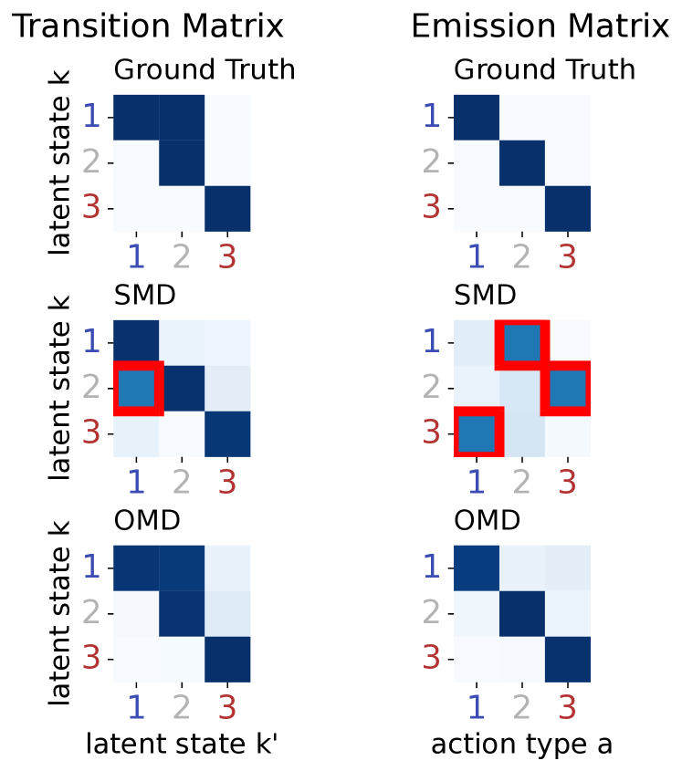
Figure 11: Recovering ground truth structures in transition and emission matrices of a state-space model. Conventionally, rows are samples independently from a (standard) Dirichlet distribution. This can result in label switching making the latent states (topics) difficult to interpret. This is particularly problematic if states are ordinal, e.g., representing “ally”, “neutral” and “enemy” relations.

The problem of “label switching” (Stephens,, 2000; Murphy,, 2012, p. 841) arises in (ad)mixture models when the indices $k$ of latent states are arbitrary, such that permuting them gives the same joint probability under the model. This issue can hamper interpretation and prevents one from averaging parameters across posterior samples without first aligning the states (e.g., using the Hungarian matching algorithm (Kuhn,, 1955)). The models we have discussed, which place an OMD prior over the emission matrix, have intrinsically ordered states that are not prone to label switching (see Fig. 11 in App. C). Although we do not view this as the main benefit of the OMD, it is a welcome side effect that facilitates easier interpretation and permits direct averaging of posterior parameters without post-hoc, potentially error-prone alignment methods.

4 MCMC INFERENCE WITH PYRO

The OMD integrates nicely with modern probabilistic programming frameworks like Pyro (Bingham et al.,, 2018; Phan et al.,, 2019). Although we do not have an analytic form for its PDF, we are able to build and perform efficient gradient-based MCMC on a range of OMD-based models by implementing Algorithm 1. We regard the OMD as a modeling motif that blends white- and black-box approaches in a way that was only recently made feasible by advances in scientific computing.

We use Pyro’s implementation of the No-U-Turn Sampler (NUTS, Hoffman and Gelman,, 2014), a variant of Hamiltonian Monte Carlo (HMC, Duane et al.,, 1987), to perform approximate posterior inference in OMD-based models. As with any MCMC method, this returns a set of $S$ posterior samples of model parameters $\{\Pi^{(s)},\Phi^{(s)},\dots\}_{s=1}^{S}$ which collectively approximate the posterior distribution. In practice, we take $S=$$1000$ samples after $200$ burn-in samples.

NUTS relies on first-order gradient information of the model’s unnormalized log joint density. Our implementation in Pyro takes gradients of the OMD density implicitly via backpropagation through the stick-breaking construction. Although the sort operation is not fully differentiable, it is piece-wise linear and sub-differentiable (Boyd and Vandenberghe,, 2004; Blondel et al.,, 2020; Tim Vieira,, 2021). We can view sort as a combination of two operations: first the non-differentiable argsort obtains permutation indices, then the differentiable gather applies the permutation. In the backward pass, the permutation of indices is simply reversed to match their original positions, obviating the need to differentiate through argsort. For this reason, the sorting of Beta variates in the construction of the OMD does not hinder gradient-based MCMC methods for inference.

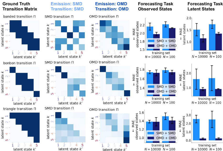
Figure 4: SMD versus OMD at forecasting. Column 1: Stylized ground-truth transition matrices. Columns 2-3: OMD recovers the transition matrices while the SMD suffers from label switching. Columns 4: OMD is better at forecasting than SMD but worse at imputation. Columns 5: OMD recovers the latent states while the SMD suffers from label switching.

5 SYNTHETIC DATA EXPERIMENTS

We conduct experiments with synthetic data to better understand and evaluate the behavior of SSMs with OMD priors. In particular, we generate datasets using hidden Markov models (HMMs) with roughly diagonal emission matrices and a range of stylized transition matrices—i.e., “banded”, “bonbon” and “triangle”, all displayed in the left column of Fig. 4. The “bonbon”, for instance, represents a realistic scenario for political event data, where “neutral” states fluctuate but “ally” and “enemy” states are nearly absorbing. To each of these datasets, we fit an HMM with OMD priors and compare its performance to a baseline HMM with SMD priors.

We generate multiple datasets for each parameter setting using $10$ random seeds, where each dataset comprises $N=$ $10000$ sequences of length $T=10$, and where a single observation takes one of $A=10$ ordinal values. We further consider two settings: one with all $N=$ $10000$ sequences and a few-shot setting where models are fit to only $N=100$. We also generate random train-test splits to evaluate two different forms of prediction:

1. Imputation: We mask a random $30$% of all observations which models impute during inference.

2. Forecasting: We designate the first $70$% of time steps for training and the latter $30$% for testing. Models are fit to the training set, then used to forecast the test observations.

Qualitative Results.

We first compare how well the two models recover known ground-truth latent structure. As expected, the OMD model reliably recovers the shape of the true transition matrix while the SMD model does not, often exhibiting label switching; see the first 3 columns of Fig. 4 for examples. As a simple quantitative measure of this, we can also calculate the mean absolute error (MAE) between the true latent states and the inferred ones. The last column of Fig. 4 reports the error on forecasting future latent states where the OMD model is substantially better; this is unsurprising and simply confirms that the OMD’s states are well-ordered while the SMD’s are label-switched.

Predictive Results.

The $4^{\textrm{th}}$ column of Fig. 4 reports MAE on forecasting future observations. The OMD model performs at least as well as the SMD model in all settings, and sometimes substantially better, as when the true transition matrix is banded ($1^{\textrm{st}}$ row). By contrast, the imputation results in Fig. 14 in App. C show the OMD model performing substantially worse than the SMD model in most settings. We speculate that the strong inductive bias imparted by the OMD prior helpfully regularizes the model’s forecasts while overly restricting its imputation ability. Intriguingly, the one setting where the OMD model has superior imputation performance is when the true transition matrix is banded, which accords with the forecasting results.

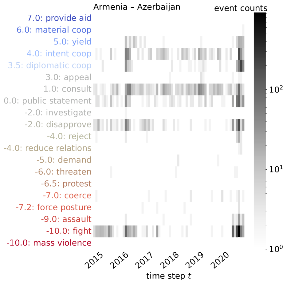
Figure 5: ICEWS event data showing interactions between Armenia and Azerbaijan over monthly time steps.

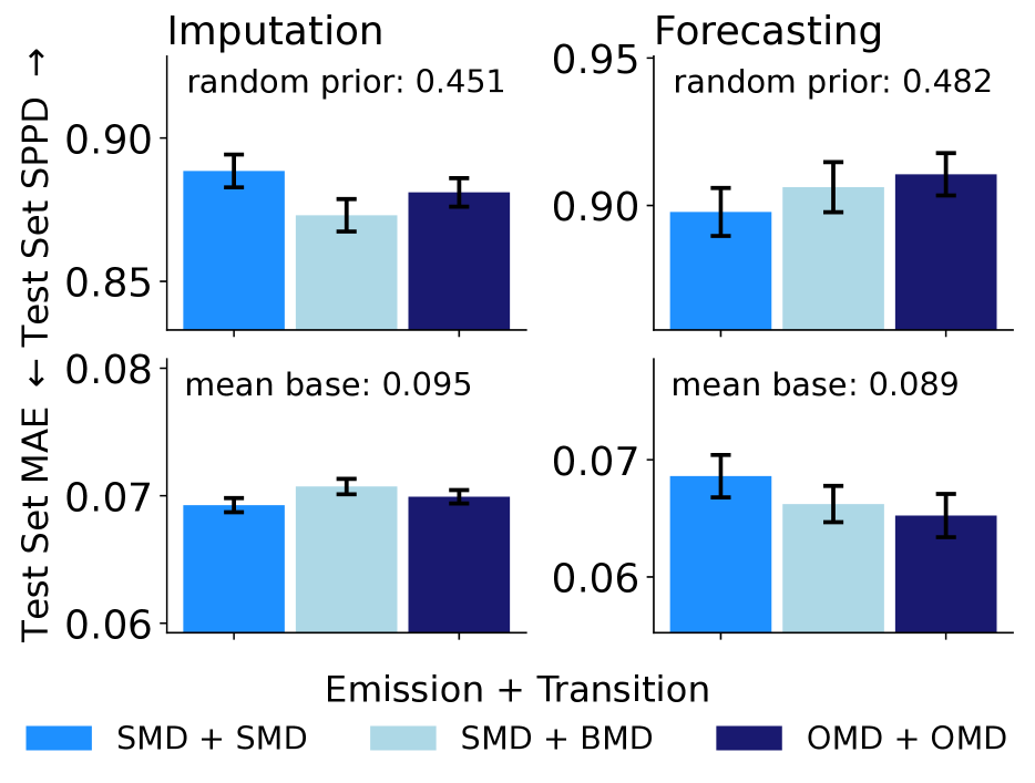
Figure 6: Imputation and forecasting evaluation on held-out ICEWS data, over $10$ runs with random seed. We fit the DPT model with different parametrizations (SMD, BMD, OMD) of the emission $\Phi$ and transition $\Pi$ matrix. We find that OMD does not significantly reduce predictive results suggesting that the imposed constraints fit the given data.

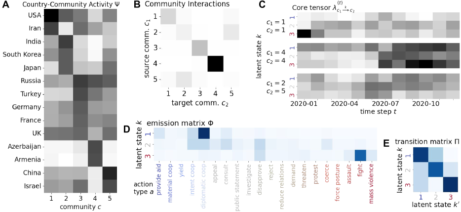
Figure 7: Posterior mean of parameters of Dynamic Poisson Tucker model fitted to ICEWS subset of 2020. (A) The latent matrix $\Psi$ indicates country-community activity. Armenia and Azerbaijan are standing out as they are involved mostly in one community (B) Interactions between latent communities. We find that communities $c=1$, $c=3$ and $c=4$ predominantly interact between themselves. (C) Selected community interactions over time: $c_{1}=4\rightarrow c_{2}=4$ are in conflict, while $c_{1}=2\rightarrow c_{2}=5$ are mostly neutral. (D) Latent emission matrix $\Phi$ representing global state-to-action probabilities. Thanks to the ordering, we know that state $k=3$ represents conflictual relationships. (E) Latent transition matrix $\Pi$ representing smooth state-to-state transition probabilities.

6 CASE STUDY: POLITICAL EVENTS

In this section, we give a case study on building an OMD-based SSM to analyze international relations event data.

6.1 ICEWS Political Events Data

We consider political event data from the Integrated Crisis Early Warning System (ICEWS) dataset (Boschee et al.,, 2015). ICEWS event data comprise millions of micro-records of the form “country $i$ took action $a$ to country $j$ at time $t$” that are machine-extracted from digital news archives. The country actors $i$ and $j$ and action types $a$ are coded to follow the Conflict and Mediation Event Observations (CAMEO) ontology (Schrodt,, 2012).

Ordered Actions

CAMEO specifies $20$ high-level action types, depicted in Fig. 5, that are naturally ordered on a conflictual-to-cooperative axis—specifically, they are each assigned a value on the expert-elicited Goldstein scale (Goldstein,, 1992), where the most cooperative action, “provide aid”, has a value of $+7.0$, and the most conflictual action, “use unconventional mass violence”, has a value of $-10.0$.

4-mode Count Tensor

Following Schein et al., 2016b , we represent the data as a count tensor ${\boldsymbol{Y}}\in\mathbb{N}_{0}^{V\times V\times A\times T}$, where an element $y^{(t)}_{i\xrightarrow{a}j}$ is the number of times country $i$ took action $a$ to country $j$ during time step $t$. We consider $V=249$ countries, $A=20$ action types (ordered by Goldstein values), and $T=72$ months. The $A\times T$ slice of this tensor corresponding to all interactions between $i\equiv\textsc{Armenia}$ and $j\equiv\textsc{Azerbaijan}$ is visualized in Fig. 5.

6.2 Dynamic Poisson Tucker model

Our model assumes each count $y^{(t)}_{i\xrightarrow{a}j}$ is Poisson distributed:

$$y^{(t)}_{i\xrightarrow{a}j} \sim\textrm{Pois}\left(\delta_{a}\,\delta^{(t)}\sum_{k=1}^{K}\lambda^{(t)}_{i\xrightarrow{k}j}\underbrace{\phi_{ka}}_{\text{emission}}\right)$$ (5)

where $\phi_{ka}$ is an entry in the state-to-action emission matrix, the parameters $\delta_{a}$ and $\delta^{(t)}$ are action- and time-scaling coefficients, and $\lambda^{(t)}_{i\xrightarrow{k}j}$ represents how well the $k^{\textrm{th}}$ state describes the relationship $(i\rightarrow j)$ at time $t$. Eq. 5 conforms to the basic form given in Eq. 1, where here the measurements and states are specifically tensor-valued.

Our model further assumes that $\lambda^{(t)}_{i\xrightarrow{k}j}$ decomposes so that

$$\sum_{k=1}^{K}\lambda^{(t)}_{i\xrightarrow{k}j}\phi_{ka}\equiv\sum_{c_{1}=1}^{C}\psi_{c_{1}i}\sum_{c_{2}=1}^{C}\psi_{c_{2}j}\sum_{k=1}^{K}\lambda^{(t)}_{c_{1}\xrightarrow{k}c_{2}}\phi_{ka}$$ (6)

where $\psi_{c_{1}i}$ and $\psi_{c_{2}j}$ represent the rate at which countries $i$ and $j$ participate in latent communities $c_{1}$ and $c_{2}$, respectively, and $\lambda^{(t)}_{c_{1}\xrightarrow{k}c_{2}}$ then represents how well the $k^{\textrm{th}}$ state describes the inter-community relationship $(c_{1}\rightarrow c_{2})$ at time $t$. The multilinear form in Eq. 6 corresponds to a Tucker decomposition Tucker, (1964), where the $\lambda^{(t)}_{c_{1}\xrightarrow{k}c_{2}}$ values collectively form the core tensor $\boldsymbol{\Lambda}^{(t)}\in\mathbb{R}_{+}^{C\times C\times K}$ at time $t$. In this setting, the core tensor can also be interpreted as a tensor-valued state (of the whole system).

We then model the evolution of the core tensor over time as

$$\lambda^{(t)}_{c_{1}\xrightarrow{k}c_{2}} \sim\textrm{Gam}\left(\tau_{0}\,\sum_{k^{\prime}=1}^{K}\lambda^{(t-1)}_{c_{1}\xrightarrow{k^{\prime}}c_{2}}\underbrace{\pi_{k^{\prime}k}}_{\text{transition}},\,\tau_{0}\right)$$ (7)

which follows the form of Poisson–Gamma Dynamical Systems (Schein et al., 2016a, ) while conforming to Eq. 2.

We place non-informative gamma priors over the parameters $\delta_{a},\,\psi_{c_{1}i},\,\psi_{c_{2}j}\stackrel{{\scriptstyle\textrm{iid}}}{{\sim}}\textrm{Gam}(\alpha_{0},\alpha_{0})$, a dynamic prior over $\delta^{(t)}\sim\textrm{Gam}(\tau_{0}\delta^{(t\!-\!1)},\,\tau_{0})$, and set $\tau_{0}=\alpha_{0}=1$.

Finally, with all of the aforementioned structure the same, we then consider three different settings for the priors over the transition $\Pi$ and emission $\Phi$ matrices: (1) OMD+OMD, where both are drawn from the OMD, (2) SMD+SMD, where both are drawn from the SMD, and (3) SMD+BMD, where $\Phi$ is drawn from the SMD and $\Pi$ is drawn from the Banded Matrix Dirichlet (BMD), as defined in § B.2.

6.3 Experiments and Results

To further understand and evaluate the OMD we fit the three above-mentioned versions of the Dynamic Poisson Tucker (DPT) model to ICEWS data and compare their qualitative and predictive performance. We use the same hyperparameters for all models with $C=5$ and $K=3$.

Predictive Evaluation

Following the design in § 5, we create $10$ train-test splits that randomly mask observations for imputation and withhold later time steps for forecasting. In addition to MAE, we evaluate performance using scaled pointwise predictive density (SPPD), a measure between $0$ and $1$ where higher is better, which we define in § B.3.

Fig. 6 reports the imputation and forecasting results for each of the three models. As in the synthetic experiments, we see that the OMD model is better than the SMD at forecasting but worse at imputation. Similarly, the BMD model is also better than the SMD at forecasting but worse at imputation. This strengthens our belief that the OMD’s inductive bias regularizes its forecasts while overly restricting its imputation ability, since the BMD exhibits the same pattern, and their two inductive biases are similar. That being said, the OMD is much more flexible than the BMD, which may explain why it outperforms the BMD in both forecasting and imputation.

Qualitative Exploration

To qualitatively inspect its inferred latent structure, we fit the OMD model to the fully-observed dataset. Fig. 7 visualizes the posterior mean of inferred model parameters for the time period of 2020. Since the model is not prone to label switching, we can inspect the posterior mean, as opposed to inspecting single (often arbitrary) sample. Fig. 7A visualizes the country-community matrix $\Psi$. We observe that Armenia and Azerbaijan are predominantly involved in community $c=4$. By visualizing a slice of the core tensor in Fig. 7B, we see that this community mostly interacts with itself. By visualizing in Fig. 7C the slice $\lambda^{(t)}_{4\xrightarrow{k}4}$, we see which states $k$ best describe community $c=4$’s self-interactions over time. In mid 2020, the most active state is $k=3$. We immediately know it represents a conflictual relationship since its index $k$ is high. This is confirmed by the emission matrix in Fig. 7D where we see that state $k=3$ places most of its mass on “fight”. Finally, we visualize the transition matrix in Fig. 7E and find that, unfortunately, transitioning out of state $k=3$ seems unlikely.

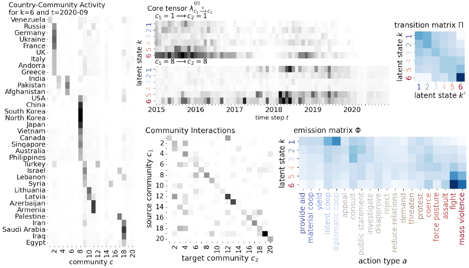
Figure 9: Posterior mean of parameters of Dynamic Poisson Tucker model, with $K=6$ latent states and $C=20$ latent communities, fitted to full temporal range (2015-2020) of ICEWS data. We find that the probability mass of the transition matrix is centered along the diagonal revealing step-wise (de-)escalatory dynamics. There is high probability of staying in state $k=6$ indicating that conflictual relationships may be hard to escape. The country-community affiliation matrix $\Psi$ provides no information on whether communities represent allies or enemies per se. To obtain this information, we interact the country-community matrix with the core tensor $\psi^{(\rightarrow)}_{c_{1}i}\sum_{c2=1}^{C}\sum_{j=1}^{V}\psi^{(\leftarrow)}_{c_{2}j}\lambda^{(t)}_{c_{1}\xrightarrow{k}c_{2}}$ for specific choice of $k$ and $t$.

We also visualize inferred latent structure from a DPT model with $K=6$ and $C=20$ fitted to ICEWS data from a longer time range 2015–2020 and present the results in Fig. 9.

7 DISCUSSION

International Relations

As alluded to throughout, this work was largely motivated by datasets, modeling approaches, and core concepts in the field of international relations (IR). The notion of escalation—that countries only gradually transition to conflict through an orderly sequence of intermediate states—is fundamental to how scholars organize and understand political events (Davis and Stan, 1984b, ). Theoretical accounts for why countries fight attempt to characterize a sequence of intermediate states that rational actors would transition through on their way to war (Snyder,, 1984; Fearon,, 1995; Jervis,, 2017). A similar perspective underlies empirical approaches. The earliest attempts to digitize international affairs into “event data” were explicitly couched in the framework of escalation—the very first sentence of Azar, (1980) reads: “As students of politics and political science, we should and we do care about the events which lead to war…”

The principal challenge in the data-intensive study of international relations is the inherent sparsity and missingness of event data, which provide only a scattered glimpse at the underlying structures we seek to reason about. This paper follows an empirical tradition of encoding strong inductive biases into statistical models of event data which encourage their inferred structure to accord with theoretical notions, like “escalation” (Schrodt,, 2006; Anders,, 2020; Randahl and Vegelius,, 2022). While much of the previous work focuses on constraining (specifically, banding) the transition structure between “states” to encourage orderly dynamics, the key idea in this paper is to draw further on the ordinal nature of observed action types. There is a steadily-growing literature on models for dyadic event data that has made exciting advances while still mostly treating action types as unordered (O’Connor et al.,, 2013; Schein et al.,, 2015; Minhas et al.,, 2016). In parallel, there has been recent work on inferring latent intensity scales Terechshenko, (2020); Stoehr et al., (2022) that imbue actions with a richer or more data-driven sense of ordering. We are eager for these threads to continue to cross, as they have in this work.

Other Models and Other Domains

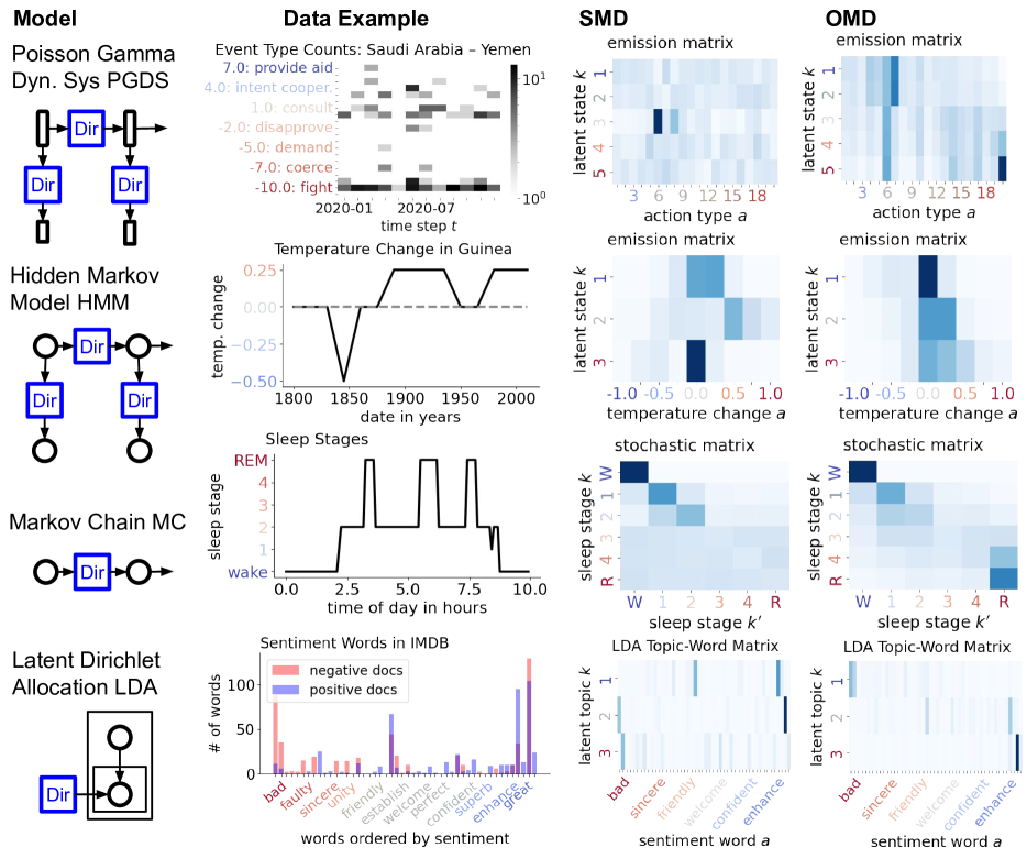
Figure 8: Different models with Dirichlet-sampled latent matrices fitted on data exhibiting ordinal dynamics. The Latent Dirichlet Allocation (LDA) has no temporal dimension, but similarly comprises a stochastic matrix describing word distributions per latent topic. If we order the observed vocabulary of words by the words’ sentiment score, the Ordered Matrix Dirichlet (OMD) can recover topics representative of sentiment levels. In all settings, we find that the OMD yields more easily interpretable stochastic matrices than the Standard Matrix Dirichlet (SMD).

The Ordered Matrix Dirichlet as a modeling motif is applicable beyond international relations and SSMs. We include in App. C a brief exploration of other OMD-based models we have built, with illustrative results on other datasets. Building these models in Pyro is easy, often only requiring a few lines of code, which facilitates this exploration. Fig. 8 summarizes four different models, all of which (and more) are available in the code we have open-sourced; we describe them here too.

1. We build an ordered form of Poisson–Gamma Dynamical Systems (PGDS) (Schein et al., 2016a, ) placing an OMD prior over the transition and emission matrices. PGDS was originally introduced to model ICEWS data, but treats actions as unordered.

2. We use an HMM with OMD-distributed emission and transition matrices to model the observed global change of temperature. In this model, noisy temperature changes are related to ordered latent states indicative of “warming” and “cooling” periods that transition gradually.

3. Even simpler, we experiment with a Markov chain model consisting of a single state-to-state transition matrix to model sleep cycles. Sleep cycles typically transition step-by-step from wake (W) to rapid eye movement (REM) stages (Pan et al.,, 2012).

4. We modify Latent Dirichlet Allocation (LDA) (Blei et al.,, 2003) to place an OMD prior over the topic-word matrix. While word types are canonically viewed as unordered, we imbue them with ordering by sorting them on “semantic axes” (An et al.,, 2018), for instance from negative to positive words. The model then infers ordered topics that reflect this semantic axis, similar to the model of Stoehr et al., (2023).

We can imagine many more applications that motivate well-ordered state-space models, like modeling product life cycles (Arvidsson,, 2019) or customer-company relationships (Netzer et al.,, 2008). Beyond SSMs, admixture models, like LDA, are fundamentally based on stochastic matrices and used in population genetics (Pritchard et al.,, 2000), stochastic block models (Airoldi et al.,, 2008), recommender systems (Gopalan et al.,, 2015), among many other areas.

8 CONCLUSION

This paper introduced the Ordered Matrix Dirichlet (OMD) distribution as a prior distribution over well-ordered stochastic matrices in state-space models (SSMs). Models built on the OMD have intrinsically ordered states that reflect ordering in the observed data. These models are more readily interpretable and usable, as they are not prone to label switching, while still being competitive on predictive tasks. The OMD integrates nicely with modern probabilistic programming frameworks, making it easy to build and fit OMD-based models. While this paper’s motivation is rooted in the concepts and data of international relations, the motifs presented here have broad applicability to domains with ordinal data and models based on stochastic matrices.

Acknowledgments

We would like to thank Kevin Du and the anonymous reviewers for valuable feedback on the manuscript and Tim Vieira for his input on order statistics and sorting. Niklas Stoehr is supported by the Swiss Data Science Center (SDSC).

Appendix A IMPACT STATEMENT

We emphasize that our models are intended for research purposes and empirical insights. They should not be blindly deployed for automated decision-making processes. The used ICEWS data may contain biases that are potentially reinforced by our modeling assumptions. The experiments with real-world event data in § 6.3 were conducted on an NVIDIA TITAN RTX GPU. The experiments with synthetically generated data in § 5 can be run on a local M1 CPU with $64$ GB of RAM in less than $10$ minutes. Limiting factors are the selected hyperparameter sizes for the latent states $K$ and communities $C$, as well as the number of time series $N$ and their length $T$. We discuss further model limitations in § 8 and § 3.

Appendix B SUPPLEMENTARY TECHNICAL DETAILS

B.1 Proof of Proposition 3.1

Proposition B.1 (OMD random variables are well-ordered).

The OMD has support over only row-stochastic matrices that obey the ordering property given beneath Eq. 3, such that for any two rows $k<k^{\prime}$ and any $a$

$$\sum_{a^{\prime}\leq a}\phi_{ka^{\prime}}\geq\sum_{a^{\prime}\leq a}\phi_{k^{\prime}a^{\prime}}$$ (8)

Proof: For $a=1$, $\phi_{k1}>\phi_{k^{\prime}1}$ is true by construction (line 5 of Algorithm 1). For $a=2$, by the definition in line 12, $\phi_{k2}=(1-\phi_{k1})\,\beta_{k2}$, and therefore the CDF at $a=2$ equals $\phi_{k1}-\phi_{k1}\beta_{k2}+\beta_{k2}$. It suffices to show that $\phi_{k1}-\phi_{k1}\beta_{k2}+\beta_{k2}>\phi_{k^{\prime}1}-\phi_{k^{\prime}1}\beta_{k^{\prime}2}+\beta_{k^{\prime}2}$, since the remaining $a>2$ then follow by induction. Re-arranging terms, $(\phi_{k1}\!-\!\phi_{k^{\prime}1})+(\beta_{k2}\!-\!\beta_{k^{\prime}2})>(\phi_{k1}\beta_{k2}-\phi_{k^{\prime}1}\beta_{k^{\prime}2})$, which follows since we know by construction that $\beta_{k2}>\beta_{k^{\prime}2}$ (line 10), and all terms $\phi_{k1},\phi_{k^{\prime}1},\beta_{k2},\beta_{k^{\prime}2}$ are between 0 and 1.

B.2 Details of the Banded Matrix Dirichlet (BMD)

In this section, we elaborate on the Banded Matrix Dirichlet (BMD). For simplicity, we consider a square matrix $\Pi\in[0,1]^{K\times K}$, but the BMD can be non-square as well. We assume that the $k^{\textrm{th}}$ state can only be excited by its directly neighboring states, $(k-1)^{\textrm{th}}$ and $(k+1)^{\textrm{th}}$, as well as by itself (Schrodt,, 2006; Randahl and Vegelius,, 2022). This results in a matrix whose non-zero elements are banded along the diagonal following:

$$\pi_{kk^{\prime}}=\begin{cases}\pi_{k}^{{(\nearrow)}}&\textrm{ if }k^{\prime}=k+1\,\,\textrm{ (escalating)}\\ \pi_{k}^{{(\searrow)}}&\textrm{ if }k^{\prime}=k-1\,\,\textrm{ (descalating)}\\ \pi_{k}^{{(\circ)}}&\textrm{ if }k^{\prime}=k\,\,\textrm{ (steady)}\\ 0&\textrm{ otherwise }\end{cases}$$ (9)

Finally, we place a Dirichlet prior over the three non-zero elements in each $k^{\textrm{th}}$ row

$$(\pi_{k}^{{(\nearrow)}},\pi_{k}^{{(\searrow)}},\pi_{k}^{{(\circ)}}) \sim\textrm{Dir}(\alpha_{0}^{{(\nearrow)}},\alpha_{0}^{{(\searrow)}},\alpha_{0}^{{(\circ)}})$$ (10)

Moreover, we can consider a wider bandwidth $b\geq 1$ so that components $k^{\prime}\in\{k-b,\dots,k+b\}$ all excite $k$. An example of the full vector might then look like

$${\boldsymbol{\pi}}_{k}=(0,\dots,0,\pi_{k}^{{(\searrow)}},\pi_{k}^{{(\circ)}},\pi_{k}^{{(\nearrow)}},0,\dots,0)$$ (11)

B.3 Details on the Scaled Pointwise Predictive Density

Scaled pointwise predictive density (SPPD) is defined as

$$\textrm{SPPD}=\exp\Big{(}\tfrac{1}{|\mathcal{I}|}\sum_{\mathbf{i}\in\mathcal{I}}\log\Big{[}\tfrac{1}{S}\sum_{s=1}^{S}\textrm{Pois}\big{(}y_{\mathbf{i}};\,\mu_{\mathbf{i}}^{(s)}\big{)}\Big{]}\Big{)}$$ (12)

where $\mathbf{i}$ is the multi-index of an entry $y_{\mathbf{i}}$ in the tensor—e.g., $\mathbf{i}=(i,j,a,t)$—and $\mathcal{I}$ is the set multi-indices corresponding to all entries in the test set. The term $\mu_{\mathbf{i}}^{(s)}$ is the Poisson rate in Eq. 5 as given by the $s^{\textrm{th}}$ posterior sample of model parameters. SPPD is the same as LPPD (Gelman et al.,, 2014), but scaled by $\tfrac{1}{|\mathcal{I}|}$ and exponentiated so it is always between 0 and 1, where higher is better.

B.4 Relevant Links

Code accompanying this paper
https://github.com/niklasstoehr/ordered-matrix-dirichlet
Integrated Crisis Early Warning System (ICEWS)
https://dataverse.harvard.edu/dataverse/icews
Goldstein Scale
https://parusanalytics.com/eventdata/cameo.dir/CAMEO.SCALE.txt
Conflict and Mediation Event Observations (CAMEO)
https://parusanalytics.com/eventdata/cameo.dir/CAMEO.09b6.pdf

Appendix C SUPPLEMENTARY PLOTS

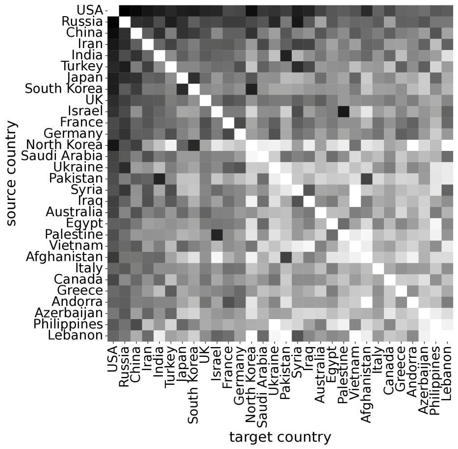
Figure 10: Descriptive statistics showing total number of interactions between countries in ICEWS data from 2015 to 2020. The rows and columns are sorted by the total number of actions a country is involved in. Note that we omit self-targeted actions as indicated by the blank diagonal.

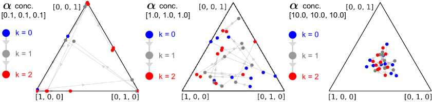
Figure 12: Samples from the Standard Matrix Dirichlet (SMD). Each point in the triangle plot represents a sample from a Dirichlet over $A=3$ classes. The $K=3$ points connected by a line represent an (unordered) sample from the SMD.

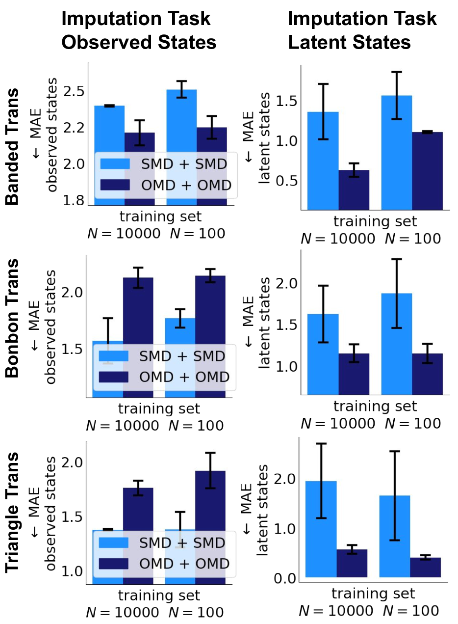
Figure 13: Imputation results of synthetic data experiments. As discussed in § 5, we generate time series with different ground truth transition structures: “banded”, “bonbon”, “triangle”. We fit a Hidden Markov Model (HMM) to a train set of these data and evaluate imputation performance on a test set. In contrast to the forecasting experiments (Fig. 4), SMD + SMD outperforms OMD + OMD in two out of three cases on observed states. In contrast to forecasting, imputation does not necessarily require a model with temporal dynamics and the ordered transition matrix does not help. As expected, OMD + OMD performs better at imputing latent states because it circumvents label switching.

action type a	action name	Goldstein value
0	provide aid	7.0
1	engage material cooperation	6.0
2	yield	5.0
3	express intent cooperate	4.0
4	engage diplomatic cooperation	3.5
5	appeal	3.0
6	consult	1.0
7	make public statement	0.0
9	investigate	-2.0
10	disapprove	-2.0
11	reject	-4.0
12	reduce relations	-4.0
13	demand	-5.0
14	threaten	-6.0
15	protest	-6.5
16	coerce	-7.0
17	exhibit force posture	-7.2
18	assault	-9.0
19	fight	-10.0
20	unconventional mass violence	-10.0

Figure 14: Ordered CAMEO action types with assigned Goldstein values. We order action types by Goldstein value first and, in case of a tie, by CAMEO ID second.

References

- Airoldi et al., (2008) Airoldi, E. M., Blei, D., Fienberg, S., and Xing, E. (2008). Mixed membership stochastic blockmodels. Advances in neural information processing systems, 21.
- An et al., (2018) An, J., Kwak, H., and Ahn, Y.-Y. (2018). SemAxis: A lightweight framework to characterize domain-specific word semantics beyond sentiment. In Proceedings of the 56th Annual Meeting of the Association for Computational Linguistics, volume 1.
- Anders, (2020) Anders, T. (2020). Territorial control in civil wars: Theory and measurement using machine learning. Journal of Peace Research, 57(6):701–714.
- Arvidsson, (2019) Arvidsson, R. (2019). On the use of ordinal scoring scales in social life cycle assessment. The International Journal of Life Cycle Assessment, 24(3):604–606.
- Azar, (1980) Azar, E. E. (1980). The conflict and peace data bank (copdab) project. Journal of Conflict Resolution, 24(1):143–152.
- Bingham et al., (2018) Bingham, E., Chen, J. P., Jankowiak, M., Obermeyer, F., Pradhan, N., Karaletsos, T., Singh, R., Szerlip, P., Horsfall, P., and Goodman, N. D. (2018). Pyro: Deep universal probabilistic programming. Journal of Machine Learning Research.
- Blei et al., (2003) Blei, D. M., Ng, A. Y., and Jordan, M. I. (2003). Latent Dirichlet allocation. Journal of Machine Learning Research, 3:993–1022.
- Blondel et al., (2020) Blondel, M., Teboul, O., Berthet, Q., and Djolonga, J. (2020). Fast differentiable sorting and ranking. International Conference on Machine Learning.
- Boschee et al., (2015) Boschee, E., Lautenschlager, J., O’Brien, S., Shellman, S., Starz, J., and Ward, M. (2015). ICEWS Coded Event Data.
- Boyd and Vandenberghe, (2004) Boyd, S. and Vandenberghe, L. (2004). Convex optimization. Cambridge University Press.
- Davidson, (2017) Davidson, R. (2017). Stochastic dominance. In The New Palgrave Dictionary of Economics, pages 1–7.
- (12) Davis, P. K. and Stan, P. (1984a). Concepts and Models of Escalation. RAND Corporation.
- (13) Davis, P. K. and Stan, P. J. E. (1984b). Concepts and models of escalation: A report from the Rand Strategy Assessment Center. Rand.
- Duane et al., (1987) Duane, S., Kennedy, A. D., Pendleton, B. J., and Roweth, D. (1987). Hybrid Monte Carlo. Physics Letters B, 195(2):216–222.
- Fearon, (1995) Fearon, J. D. (1995). Rationalist explanations for war. International organization, 49(3):379–414.
- Gelman et al., (2013) Gelman, A., Carlin, J. B., Stern, H. S., Dunson, D. B., Vehtari, A., and Rubin, D. B. (2013). Bayesian data analysis. Chapman and Hall/CRC.
- Gelman et al., (2014) Gelman, A., Hwang, J., and Vehtari, A. (2014). Understanding predictive information criteria for Bayesian models. Statistics and Computing, 24(6):997–1016.
- Goldstein, (1992) Goldstein, J. (1992). A conflict-cooperation scale for WEIS events data. The Journal of Conflict Resolution, 36(2):369–385.
- Gopalan et al., (2015) Gopalan, P., Hofman, J. M., and Blei, D. M. (2015). Scalable recommendation with hierarchical Poisson factorization. In UAI, pages 326–335.
- Hoffman and Gelman, (2014) Hoffman, M. D. and Gelman, A. (2014). The No-U-Turn Sampler: Adaptively setting path lengths in Hamiltonian Monte Carlo. Journal of Machine Learning Research, 15(1):1593–1623.
- Jervis, (2017) Jervis, R. (2017). Perception and misperception in international politics: New edition. Princeton University Press.
- Kalman, (1960) Kalman, R. E. (1960). A new approach to linear filtering and prediction problems. Journal of Basic Engineering, 82(1):35–45.
- Kuhn, (1955) Kuhn, H. W. (1955). The Hungarian method for the assignment problem. Naval Research Logistics Quarterly, 2(1-2):83–97.
- Minhas et al., (2016) Minhas, S., Hoff, P. D., and Ward, M. D. (2016). A new approach to analyzing coevolving longitudinal networks in international relations. Journal of Peace Research, 53(3):491–505.
- Murphy, (2012) Murphy, K. P. (2012). Machine learning: A probabilistic perspective. MIT Press, Cambridge, MA.
- Netzer et al., (2008) Netzer, O., Lattin, J. M., and Srinivasan, V. (2008). A hidden Markov model of customer relationship dynamics. Marketing Science, 27(2):185–204.
- O’Connor et al., (2013) O’Connor, B., Stewart, B., and Smith, N. (2013). Learning to extract international relations from political context. In Proceedings of the 51st Annual Meeting of the Association for Computational Linguistics, volume 1, pages 1094–1104.
- Pan et al., (2012) Pan, S.-T., Kuo, C.-E., Zeng, J.-H., and Liang, S.-F. (2012). A transition-constrained discrete hidden Markov model for automatic sleep staging. BioMedical Engineering OnLine, 11(1):52.
- Phan et al., (2019) Phan, D., Pradhan, N., and Jankowiak, M. (2019). Composable effects for flexible and accelerated probabilistic programming in NumPyro. arXiv, 1912.11554.
- Pritchard et al., (2000) Pritchard, J. K., Stephens, M., and Donnelly, P. (2000). Inference of population structure using multilocus genotype data. Genetics, 155(2):945–959.
- Randahl and Vegelius, (2022) Randahl, D. and Vegelius, J. (2022). Predicting escalating and de-escalating violence in Africa using Markov models. International Interactions, pages 1–17.
- Richardson and Green, (1997) Richardson, S. and Green, P. J. (1997). On Bayesian analysis of mixtures with an unknown number of components. Journal of the Royal Statistical Society: Series B (Statistical Methodology), 59(4):731–792.
- Schein et al., (2015) Schein, A., Paisley, J., Blei, D. M., and Wallach, H. (2015). Bayesian Poisson tensor factorization for inferring multilateral relations from sparse dyadic event counts. In Proceedings of the 21th ACM SIGKDD International Conference on Knowledge Discovery and Data Mining, pages 1045–1054.
- (34) Schein, A., Wallach, H., and Zhou, M. (2016a). Poisson-Gamma dynamical systems. In Advances in Neural Information Processing Systems, volume 29.
- (35) Schein, A., Zhou, M., Blei, D. M., and Wallach, H. (2016b). Bayesian Poisson Tucker decomposition for learning the structure of international relations. In Proceedings of the 33rd International Conference on Machine Learning, volume 48, pages 2810–2819.
- Schrodt, (2008) Schrodt, P. (2008). Kansas event data system (KEDS).
- Schrodt, (2012) Schrodt, P. (2012). CAMEO: Conflict and mediation event observations event and actor codebook. Parus Analytics.
- Schrodt, (2006) Schrodt, P. A. (2006). Forecasting conflict in the Balkans using hidden Markov models. In Programming for Peace, pages 161–184. Springer Netherlands.
- Snyder, (1984) Snyder, G. H. (1984). The security dilemma in alliance politics. World politics, 36(4):461–495.
- Stephens, (2000) Stephens, M. (2000). Dealing with label switching in mixture models. Journal of the Royal Statistical Society: Series B (Statistical Methodology), 62(4):795–809.
- Stoehr et al., (2023) Stoehr, N., Cotterell, R., and Schein, A. (2023). Sentiment as an ordinal latent variable. In European Chapter of the ACL (EACL).
- Stoehr et al., (2022) Stoehr, N., Hennigen, L. T., Valvoda, J., West, R., Cotterell, R., and Schein, A. (2022). An ordinal latent variable model of conflict intensity. In arXiv, volume 2210.03971.
- Terechshenko, (2020) Terechshenko, Z. (2020). Hot under the collar: A latent measure of interstate hostility. Journal of Peace Research, 57(6):764–776.
- Tim Vieira, (2021) Tim Vieira (2021). On the distribution function of order statistics.
- Tucker, (1964) Tucker, L. R. (1964). The extension of factor analysis to three-dimensional matrices. In Gulliksen, H. and Frederiksen, N., editors, Contributions to mathematical psychology., pages 110–127. Holt, Rinehart and Winston.