From topological phase to Anderson localization in a two-dimensional quasiperiodic system

Abstract

In this paper, the influence of the quasidisorder on a two-dimensional system is studied. We find that there exists a topological phase transition accompanied by a transverse Anderson localization. The topological properties are characterized by the band gap, the edge-state spectra, the transport conductance, and the Chern number. The localization transition is clearly demonstrated by the investigations of the partial inverse participation ratio, the average of level spacing ratio, and the fraction dimension. The results reveal the topological nature of the bulk delocalized states. Our work facilitates the understanding on the relationship between the topology and the Anderson localization in two-dimensional disordered systems.

Introduction.—

Band insulators have attracted much attention because of their peculiar topological properties. Two representative insulators are the Chern class Haldane (1988) and the quantum spin-Hall class Kane and Mele (2005); Hasan and Kane (2010); Qi and Zhang (2011). The topological properties are reflected in that although these band insulators present the characteristics of an insulator in the bulk, there still exists robust conducting states, distributed at the edges of the band insulators. The Fermi levels of these edge modes connect the valence and conduction bands, making the insulators present metallic characteristics Nagaosa et al. (2010). Moreover, the presence or absence of the edge modes can be predicted by the Chern number ($C$). According to the Thouless-Kohmoto-Nightingale-den Nijs (TKNN)’s work Thouless et al. (1982), $C\neq 0$ indicates the presence of the edge modes, whereas $C=0$ means the absence of the edge modes.

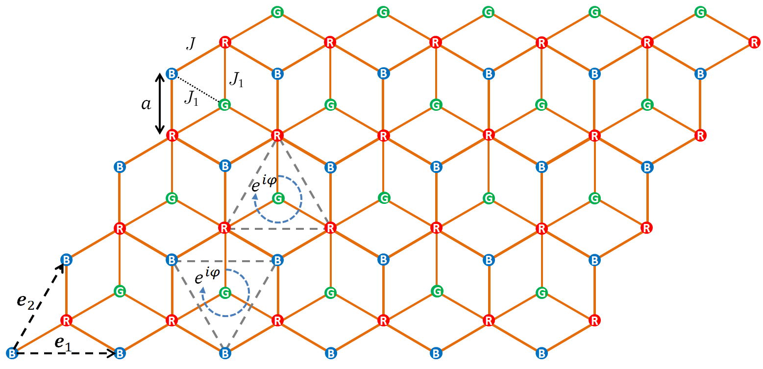
Figure 1: (Color Online) Sketch of the model. The primitive lattice vectors $\bm{e_{1}}$ and $\bm{e_{2}}$ form a unit cell, which contains three types of independent sublattices, marked by $\rm{R}$, $\rm{B}$, and $\rm{G}$, respectively. The hopping strength between nearest neighbor $\rm{R}$ and $\rm{B}$ sites is $J$, and the one between nearest neighbor $\rm{G}$ and $\rm{R}$ (or $\rm{B}$) sites is $J_{1}$. The hopping strength between two nearest neighbor $\rm{R}$ (or $\rm{B}$) sites is $J_{2}e^{i\varphi}$.

The above mentioned metallic characteristics are found to be robust against the disorder, implying that the topological properties of the system still preserve as long as the bulk gap keeps open within a certain disorder strength Xiao et al. (2010). Increasing the disorder strength will finally lead to the close of the bulk gap, making the system be in a topologically trivial phase Prodan et al. (2010); Prodan (2011). Recently, there are growing interests in studying localization in the two-dimensional systems Abrahams et al. (1979); Liu and Das Sarma (1994); Liu et al. (1996); Xie et al. (1998); MacKinnon and Kramer (1981, 1983); Onoda and Nagaosa (2003); Onoda et al. (2007); Xu et al. (2012a); Gonçalves et al. (2018); Li et al. (2021) with Anderson disorder. Particularly, the coexistence of nontrivial topology and Anderson localization in a quantum spin-Hall system Yang et al. (2011) with broken time-reversal symmetry is found and the extended states are protected by the nontrivial topology Xu et al. (2012b). It is known to us that quasidisorder is a another form of disorder and it belongs to the correlated disorder Aubry and André (1980) and the Chern insulator is one of the types of the band insulators without time-reversal symmetry. In this work, we are motivated to investigate whether the aforementioned conclusion about the topological nature of the bulk states still applies to the quasidisordered Chern insulators. After all, Ref. Xie et al. (1998) has remarked that there may exist multifractal wave functions in the two-dimensional disordered systems.

Model.—

Figure 1 presents the schematic diagram of the two-dimensional quasidisordered Chern insulator system. The primitive lattice vectors, $\bm{e_{1}}$ and $\bm{e_{2}}$, constitute the unit cell where there are three types of independent sublattices, marked by $\rm{R}$, $\rm{B}$, and $\rm{G}$, respectively. $a$ is the spacing between two nearest neighbor sites ($a=1$ in general). The Hamiltonian ($\hat{H}$) of the system consists of two parts. One is the hopping terms ($\hat{H}_{1}$) and another is the quasidisordered (quasiperiodic) potentials ($\hat{H}_{2}$). The total Hamiltonian is $\hat{H}=\hat{H}_{1}+\hat{H}_{2}$. $\hat{H}_{1}$ reads

$$\hat{H}_{1} =\sum_{j,j^{\prime}}\left(J\hat{c}^{{\dagger}}_{\rm{R}_{j}}\hat{c}_{\rm{B}_{j^{\prime}}}+J_{1}\hat{c}^{{\dagger}}_{\rm{G}_{j}}\hat{c}_{\rm{R}_{j^{\prime}}}+J_{1}\hat{c}^{{\dagger}}_{\rm{G}_{j}}\hat{c}_{\rm{B}_{j^{\prime}}}\right.$$ (1)

$$\left.+J_{2}e^{i\varphi}\hat{c}^{{\dagger}}_{\rm{R}_{j}}\hat{c}_{\rm{R}_{j^{\prime}}}+J_{2}e^{i\varphi}\hat{c}^{{\dagger}}_{\rm{B}_{j}}\hat{c}_{\rm{B}_{j^{\prime}}}+h.c.\right),$$

where $J$ is the unit of energy and $\mathcal{S}_{m,n}=m\bm{e_{1}}+n\bm{e_{2}}$ ($m$ and $n$ are integers) is the position of the $\mathcal{S}$ site ($\mathcal{S}\in\{\rm{R},\rm{B},\rm{G}\}$). $\hat{H}_{2}$ is

$$\hat{H}_{2} =\sum_{\mathcal{S}_{m,n}}V\cos(2\pi\alpha n)\hat{c}^{{\dagger}}_{\mathcal{S}_{m,n}}\hat{c}_{\mathcal{S}_{m,n}},$$ (2)

where $V$ is the strength of the quasi-periodic potential, and $\alpha=(\sqrt{5}-1)/2$. Intuitively, this is a multi-parameter system. In this paper, we aim to investigate the topological properties, localization phase transition, and the quantum criticality cased by the quai-periodic potential. In the following, we take $J_{1}=0.3$, $J_{2}=0.275$, and $\varphi=\pi/2$ without loss of generality.

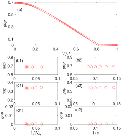
Figure 2: (Color Online) (a) The energy gap of the lower two minibands as a function of $V$ under PBC. The considered system has a size of $40\times 144$. (40 unit cells along $\bm{e_{1}}$ and $144$ unit cells along $\bm{e_{2}}$). (b1)-(d2) Finite-size analysis about the energy gap with $V=0.1J$ in (b1) and $(b2)$, $V=0.5J$ in (c1) and (c2), and $V=J$ in (d1) and (d2). To obtain (b1), (c1), and (d1), we keep $N_{\bm{e_{2}}}$ invariant and change $N_{\bm{e_{1}}}$. While calculating (b2), (c2), and (d2), we only change $N_{\bm{e_{2}}}$, and make $N_{\bm{e_{2}}}$ be equal to the $s$-th Fibonacci number. Obviously, the energy gaps almost remain constants as the size of the system increases.

Topological properties.—

Considering a system with the size $N_{\bm{e_{1}}}\times N_{\bm{e_{2}}}=40\times 144$ ($N_{\bm{e_{1}}}$ is the number of unit cells along $\bm{e_{1}}$ (the longitudinal direction) and $N_{\bm{e_{2}}}$ is the one along $\bm{e_{2}}$ (the transverse direction) and selecting periodic boundary conditions (PBC) in two directions, we plot the energy gap of the lower two minibands as a function of $V$ in Fig. 2(a). Intuitively, we can see that a critical point $V_{c}$ ($V_{c}\approx 0.82J$ in the numerical calculations) separates the system into two different phases. When the potential strength $V$ is less than the critical point, the gap is always open, whereas the gap is closed when $V$ crosses the critical point. To make it clear whether the energy gap is sensitive to the size of the system, we perform the finite-size analysis on the energy gap. Figures 2(b1) and 2(b2), 2(c1) and 2(c2), and 2(d1) and 2(d2) shows the results with $V=0.1J$, $V=0.5J$, and $V=J$, respectively. Particularly, to calculate the gaps in Figs. 2(b1), 2(c1), and 2(d1), we leave $N_{\bm{e_{2}}}$ unchanged. When calculating the gaps in 2(b2), 2(c2), and 2(d2), we keep $N_{\bm{e_{1}}}$ invariant and make $N_{\bm{e_{2}}}$ be equal to the $s$-th Fibonacci number $F_{s}$. Obviously, as the size of the system increases, the gaps almost remain constants. It implies that the energy gap is insensitive to the size of the system. Based on the energy gap, we infers that the gapped phase at $V>0$ preserves the topological characteristics of the original uniform case ($V=0$). We know that for the uniform case, its topological properties are intermediately reflected from the Bloch Chern number. That is, the TKNN formula Thouless et al. (1982) is used to characterize the topological properties of the system. In this case, the Chern number of the lowest bands will show to be $C_{1}=1$.

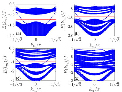
Figure 3: (Color Online) Zigzag-edge spectra $E(k_{\bm{e_{1}}})/J$ of the lowest two bands as a function of $k_{\bm{e_{1}}}$. (a) $V=0J$; (b) $V=0.3J$; (c) $V=0.5J$; (d) $V=1J$. The red solid lines are the representative Fermi levels. The size of the system is $64\times 89$.

We first try to verify the aforementioned inference by the singly periodic spectrum. The lattice size is $64\times 89$ and we leave it with PBC in the longitudinal direction and with zigzag edge in the transverse direction. Thus, the momentum $k_{\bm{e_{1}}}$ in the $\bm{e_{1}}$ direction is a good quantum number. Figure 3(a) presents the zigzag-edge spectrum in the $V=0$ case. The red line represents the $1/3$-filling fermi energy level in the bulk gap, at which there are two edge modes with opposite momentum $k_{\bm{e_{1}}}$, whose corresponding group velocities are of opposite signs. For the quasi-periodic cases, one can see that there exists two edges within the bulk gap at $1/3$ filling as well (see the cases with $V=0.3J$ and $V=0.5J$ in Figs. 3(b) and 3(c), respectively). It means that there are preserved topological characteristics in the quasi-periodic case. Nevertheless, compared to the uniform case, the corresponding momenta of the two edge modes are no longer symmetric about $k_{\bm{e_{1}}}=0$ in the quasi-periodic cases. For the $V=J$ case, there is no full bulk gap in the zigzag-edge spectrum (see Fig. 3(d)), presenting the metallic characteristics, which is self-consistent with the energy gap under PBC (see Fig. 2(a)).

Except for the edge modes, the transport conductance Li et al. (2009); Jiang et al. (2009); Groth et al. (2009); Orth et al. (2016); Song et al. (2012); García et al. (2015); Zhang et al. (2012) is an observable to characterize the topological features as well. For convenience but without loss of generality, both the (left and right) leads are described by the Hamiltonian $\hat{H}$ as well. The conductance $G_{E}$ of the system (central scattering region) can be obtained from the Landauer formula Imry and Landauer (1999); Datta (1995),

$$G_{E}=\frac{2e^{2}}{h}T_{E},$$ (3)

where $2e^{2}/h$ is the unit of $G_{E}$ and $T_{E}$ is the transmission coefficient, which is expressed as

$$T_{E}=Tr\left[\Gamma_{L}G^{r}\Gamma_{R}G^{a}\right],$$ (4)

where $G^{r}$ ($G^{a}$) is the retarded (advanced) Green’s function of the system with $G^{r}=\left[EI-H_{C}-\Sigma_{L}-\Sigma_{R}\right]$ and $G^{a}=\left(G^{r}\right)^{{\dagger}}$, and $\Gamma_{L/R}=i\left[\Sigma_{L/R}-\left(\Sigma_{L/R}\right)^{{\dagger}}\right]$. Here, we have used $H_{C}$ to denote the Hamiltonian of the system. The self-energies $\Sigma_{L}$ and $\Sigma_{R}$ are given by

$$\Sigma_{L}=H^{{\dagger}}_{LC}{\rm{g}}_{L}H_{LC},\leavevmode\nobreak\ \Sigma_{R}=H_{CR}{\rm{g}}_{R}H^{{\dagger}}_{CR},$$ (5)

where $H_{LC}$ ($H_{CR}$) denotes the coupling matrices between the system and the $L\leavevmode\nobreak\ (R)$ leads, and ${\rm{g}}_{L}$ (${\rm{g}}_{R}$) are surface Green’s functions of the $L\leavevmode\nobreak\ (R)$ leads.

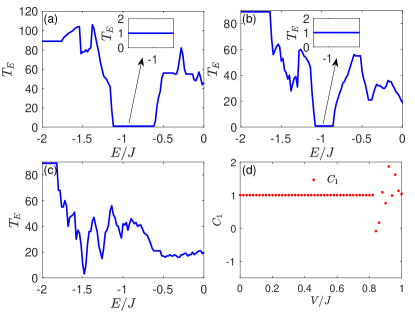
Figure 4: (Color Online) The transmission coefficient $T_{E}$ as a function of the Fermi energy with $V=0.3J$ in (a); $V=0.6J$ in (b); and $V=J$ in (c). The insets enlarge the stage with $T_{E}=1$. (d) The Chern number $C_{1}$ versus the potential strength $V$ at 1/3 filling. The size of the system is $40\times 144$.

We consider a system size $40\times 144$ with OBC in $\bm{e_{2}}$ and take $V=0.3J$, $V=0.6J$, and $V=J$. The transmission coefficients as a function the Fermi energy are presented in Figs. 4(a), 4(b), and 4(c), respectively. Apparently, in the gapped cases ($V=0.3J$ and $V=0.6J$), there is a step with $T_{E}=1$ at 1/3 filling. While in the gapless case ($V=J$), no stage with $T_{E}=1$ exists at 1/3 filling. Furthermore, the results of the $T_{E}$ are coincide with the topological phase diagram in Fig. 4(d). In this diagram, $C_{1}=1$ for $V<V_{c}$, corresponding to $T_{E}=1$, while $C_{1}$ is unquantized when the potential strength $V$ crosses the critical point $V_{c}$, corresponding to the unquantized $T_{E}$. The reason for the appearance of the unquantized Chern number is that in this parameter region, the bulk gap is actually closed. Hence, there is no topology-protected edge mode, reflecting the trivial nature of the system. On the contrary, the quantized $C_{1}=1$ exactly corresponds to the two edge modes within the bulk gap, presenting the bulk-edge correspondence, and being self-consistent with the two-channel conductance. In addition, the system can be viewed as a one-dimensional tight-binding model in the longitudinal direction, but each unit cell now is replaced by a super cell which contains $N_{\bm{e_{2}}}$ cells. When $V>V_{c}$, the one-dimensional tight-binding model describes a gapless metal. Therefore, in the gapless case, there is no quantized conductance below or above the Fermi energy at 1/3 filling (see Fig. 4(c)), presenting intrinsically metallic transport characteristics of the system.

Localization phase transition.—

The two-channel transport observation shows that there is no any edge mode and no localization phenomenon along the longitudinal direction when $V>V_{c}$. We infer that the absence of the edge mode is related with the localization in the transverse direction. After all, the localization will prevent the particles from moving towards the boundaries of the system, so that the system can not form the edge states. To confirm this conjecture, we will use the partial inverse participation ratio (PIPR) to characterize the localization properties of the system. The system has a size with $N_{\bm{e_{2}}}=F_{s}$ in the $\bm{e_{2}}$ direction while it has no limitation for $N_{\bm{e_{1}}}$, but satisfies PBC in two directions. $N_{\bm{e_{2}}}$ is chosen as the Fibonacci number to minimize the size effect. Then, the PIPR of a normalized wave function $\psi$ reads

$${\rm PIRP}=\sum^{N_{\bm{e_{2}}}-1}_{n=0}|\psi({\mathcal{S}_{n}})|^{4}N^{2}_{\bm{e_{1}}}.$$ (6)

where the index $m$ has been suppressed (the same below).

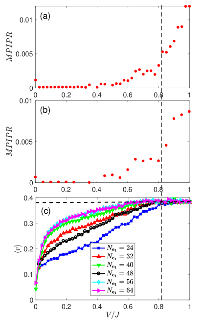
Figure 5: (Color Online) The MPIPR as function of the quasi-periodic potential strength $V$ with the system size $24\times 233$ in (a) and $24\times 377$ in (b). The averaged level spacing ratio $\langle r\rangle$ as a function of $V$ is presented in (c) with $N_{\bf e_{2}}=144$, where the horizontal black dashed line corresponds to the Poisson distribution value $\langle r\rangle\approx 0.3863$. The black dashed reference line denotes the critical point.

Since there is preserved translational invariance in the longitudinal direction, the wave packets is periodically distributed in this direction. Noting that the PIPR in Eq. (6) is a quantity defined in the transverse direction, hence, it is more convenient and effective to use the PIPR to characterize the localization property in this direction. When the PIRP tends to a finite value $O(1)$, the wave function is localized in the $\bm{e_{2}}$ direction. The PIRP scales as $F^{-1}_{s}$ for the extended states, while behaves like $F^{-\gamma}_{s}$ ($0<\gamma<1$) for the critical states. Due to the distinct difference between the localized states and the extended (or critical) states, therefore, in the following, we name the extended and the critical states as the delocalized states. Choosing two system sizes $24\times 233$ and $24\times 377$ as examples, the corresponding mean PIPR (MPIPR) of the wave functions within the 1/3 filling are plotted in Figs. 5(a) and 5(b). Intuitively, the MPIPR jumps at the critical point (the black dashed line shows), signaling a transverse delocalization-localization transition.

Next, we try to study the transverse localization transition by analyzing the energy gap statistic. To perform the analysis, we will calculate the average of the energy level spacing ratio $\langle r\rangle$ over the energies within the 1/3 filling, which is defined by $\langle r\rangle=\frac{1}{N_{\bm{e_{1}}}\times N_{\bm{e_{2}}}-2}\sum_{j}r_{j}$, where $r_{j}={\rm min}\{\delta_{j},\delta_{j+1}\}/{\rm max}\{\delta_{j},\delta_{j+1}\}$ and $\delta_{j}=E_{j+1}-E_{j}$ with the energies $E_{j}$ arranged in an ascending order. In the numerically calculations, we take PBC and $N_{\bf e_{2}}=144$. Figure. 5(c) presents $\langle r\rangle$ as a function of $V$ for various $N_{\bf e_{1}}$ at 1/3 filling. Apparently, $\langle r\rangle$ approaches the Poisson distribution value Oganesyan and Huse (2007); Pal and Huse (2010) $\langle r\rangle_{\rm Possion}=2{\rm ln}(2)-1\approx 0.3863$ (the horizontal black dashed line in Fig. 5(c) shows) when the quasidisorder strength $V$ is larger than the critical point. Besides, it is readily seen that $\langle r\rangle$ for various $N_{\bf e_{1}}$ are less than $0.3863$ when $V$ is smaller than the critical value, presenting the level statistics feature of the single-particle delocalized states Schiffer et al. (2021).

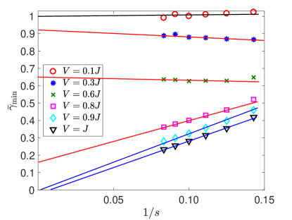
Figure 6: (Color Online) Plots of $\bar{\gamma}_{\rm min}$ versus $1/s$ for the wave functions within 1/3 filling.

Finally, to make the transverse delocalization-localization transition more clear, we analyze the scaling behavior of the wave functions. As mentioned above, the wave packets are periodically distributed at each site $\mathcal{S}_{n}$. The probability $P(\mathcal{S}_{n})$ for the sites in the transverse direction is defined as $P(\mathcal{S}_{n})=|\psi(\mathcal{S}_{n})|^{2}N_{\bm{e_{1}}}$. Then a scaling index $\gamma_{j}$ is given by $P(\mathcal{S}_{n})=F^{-\gamma_{j}}_{s}$. For a concrete wave function, $\gamma_{j}$ will distribute within a interval $\left[\gamma_{\rm min},\leavevmode\nobreak\ \gamma_{\rm max}\right]$. In the thermodynamic limit $1/s\rightarrow 0$, $\gamma_{\rm min}\rightarrow 0$ corresponds to the localized states, while $0<\gamma_{\rm min}\leq 1$ for the delocalized states (Particularly, $\gamma_{\rm min}=1$ denotes the extended states, otherwise, it corresponds to the critical states). Therefore, we will employ $\gamma_{\rm min}$ to characterize the scaling behaviors of the wave functions. In the numerical calculations, we choose $N_{\bm{e_{1}}}=40$ and take PBC and then average the $\gamma_{\rm min}$ over the wave functions whose corresponding energies are within the $1/3$ filling. We label the averaged $\gamma_{\rm min}$ by $\bar{\gamma}_{\rm min}=\frac{1}{N_{\bm{e_{1}}}\times N_{\bm{e_{2}}}}\sum^{N_{\bm{e_{1}}}\times N_{\bm{e_{2}}}}_{j=1}\gamma^{j}_{\rm min}$. The extracted $\bar{\gamma}_{\rm min}$ from the wave functions for different $V$ are plotted in Fig. 6. From this plots, it is readily seen that the $\bar{\gamma}_{\rm min}$ in the extrapolating limit decreases as the quasi-periodic potential strength $V$ increases, and it finally reduces to zero when $V$ crosses the critical point $V_{c}$, verifying the transverse delocalization-localization phase transition. The results reflected from the $\bar{\gamma}_{\rm min}$ confirms the prediction of the MPIPR and the energy gap statistics.

Summary.—

In summary, we have investigated the influence of the quasidisorder on the topological properties and the localization behaviors of a two-dimensional system. The topological phase transition is charactered by the band gap, edge-state spectra, and transport conductance. When the topological transition happens, we find that the bands gap closes, and no any edge modes exists. Meanwhile, the transport conductance shows that the system is more like a metal in the gapless phase. The results are self-consistent with the topological diagram which contains the Chern number of lowest band. In addition, a transverse localization transition is characterized by the MPIPR, level statistics, and the fraction dimension. The findings extend the insight about relationship between the topology and the localization properties of the bulk states, and the reveal the topological nature of the bulk delocalized states.

In the previous work, we have made a theoretical scheme Cheng et al. (2020) to realize the Hamiltonian $\hat{H}_{1}$ presented in Eq. (1). In this scheme, the noninteracting particles are confined in the two-dimensional lattice, and initially hop between the nearest-neighbor sites. The system is initially gapless and topological trivial. Once a circular-frequency shaking is applied, then the next-nearest hoppings are introduced and then the system becomes gapped and topological nontrivial. Experimentally, the lattice geometry has been realized by three retro-reflected lasers and the hoppings of particles are controlled by tuning the depth of the Eckardt (2017). Besides, the Floquet shaking technique has been applied to optical honeycomb lattice Jotzu et al. (2014) to realize the Haldane model Haldane (1988). In addition, the quasidisorder potential $\hat{H}_{2}$ presented in Eq. (2) has been realized by superimposing two independent lasers with different wavelengths Roati et al. (2008); M. et al. (2015); Bordia et al. (2007). As a result, we believe that the findings in this two-dimensional quasidisordered system has the potential to be observed in the ultracold atomic experiments.

We acknowledge support from NSFC under Grants No. 11835011 and No. 12174346.

References

- Haldane (1988) F. D. M. Haldane, “Model for a quantum hall effect without landau levels: Condensed-matter realization of the ”parity anomaly”,” Phys. Rev. Lett. 61, 2015 (1988).
- Kane and Mele (2005) C. L. Kane and E. J. Mele, “Quantum spin hall effect in graphene,” Phys. Rev. Lett. 95, 226801 (2005).
- Hasan and Kane (2010) M. Z. Hasan and C. L. Kane, “Colloquium: Topological insulators,” Rev. Mod. Phys. 82, 3045 (2010).
- Qi and Zhang (2011) X.-L. Qi and S.-C. Zhang, “Topological insulators and superconductors,” Rev. Mod. Phys. 83, 1057 (2011).
- Nagaosa et al. (2010) N. Nagaosa, J. Sinova, S. Onoda, A. H. MacDonald, and N. P. Ong, “Anomalous hall effect,” Rev. Mod. Phys. 82, 1539 (2010).
- Thouless et al. (1982) D. J. Thouless, M. Kohmoto, M. P. Nightingale, and M. den Nijs, “Quantized hall conductance in a two-dimensional periodic potential,” Phys. Rev. Lett. 49, 405 (1982).
- Xiao et al. (2010) D. Xiao, M.-C. Chang, and Q. Niu, “Berry phase effects on electronic properties,” Rev. Mod. Phys. 82, 1959 (2010).
- Prodan et al. (2010) E. Prodan, T. L. Hughes, and B. A. Bernevig, “Entanglement spectrum of a disordered topological chern insulator,” Phys. Rev. Lett. 105, 115501 (2010).
- Prodan (2011) E. Prodan, “Disordered topological insulators: a non-commutative geometry perspective,” Journal of Physics A: Mathematical and Theoretical 44, 113001 (2011).
- Abrahams et al. (1979) E. Abrahams, P. W. Anderson, D. C. Licciardello, and T. V. Ramakrishnan, “Scaling theory of localization: Absence of quantum diffusion in two dimensions,” Phys. Rev. Lett. 42, 673 (1979).
- Liu and Das Sarma (1994) D. Z. Liu and S. Das Sarma, “Universal scaling of strong-field localization in an integer quantum hall liquid,” Phys. Rev. B 49, 2677 (1994).
- Liu et al. (1996) D. Z. Liu, X. C. Xie, and Q. Niu, “Weak field phase diagram for an integer quantum hall liquid,” Phys. Rev. Lett. 76, 975 (1996).
- Xie et al. (1998) X. C. Xie, X. R. Wang, and D. Z. Liu, “Kosterlitz-thouless-type metal-insulator transition of a 2d electron gas in a random magnetic field,” Phys. Rev. Lett. 80, 3563 (1998).
- MacKinnon and Kramer (1981) A. MacKinnon and B. Kramer, “One-parameter scaling of localization length and conductance in disordered systems,” Phys. Rev. Lett. 47, 1546 (1981).
- MacKinnon and Kramer (1983) A. MacKinnon and B. Kramer, “The scaling theory of electrons in disordered solids: Additional numerical results,” Zeitschrift für Physik B Condensed Matter 53, 1 (1983).
- Onoda and Nagaosa (2003) M. Onoda and N. Nagaosa, “Quantized anomalous hall effect in two-dimensional ferromagnets: Quantum hall effect in metals,” Phys. Rev. Lett. 90, 206601 (2003).
- Onoda et al. (2007) M. Onoda, Y. Avishai, and N. Nagaosa, “Localization in a quantum spin hall system,” Phys. Rev. Lett. 98, 076802 (2007).
- Xu et al. (2012a) Z. Xu, L. Sheng, D. Y. Xing, E. Prodan, and D. N. Sheng, “Topologically protected extended states in disordered quantum spin-hall systems without time-reversal symmetry,” Phys. Rev. B 85, 075115 (2012a).
- Gonçalves et al. (2018) M. Gonçalves, P. Ribeiro, and E. V. Castro, “The haldane model under quenched disorder,” (2018), arXiv: 1807.11247 .
- Li et al. (2021) H. Li, C.-Z. Chen, H. Jiang, and X. C. Xie, “Coexistence of quantum hall and quantum anomalous hall phases in disordered ,” Phys. Rev. Lett. 127, 236402 (2021).
- Yang et al. (2011) Y. Yang, Z. Xu, L. Sheng, B. Wang, D. Y. Xing, and D. N. Sheng, “Time-reversal-symmetry-broken quantum spin hall effect,” Phys. Rev. Lett. 107, 066602 (2011).
- Xu et al. (2012b) Z. Xu, L. Sheng, D. Y. Xing, E. Prodan, and D. N. Sheng, “Topologically protected extended states in disordered quantum spin-hall systems without time-reversal symmetry,” Phys. Rev. B 85, 075115 (2012b).
- Aubry and André (1980) S. Aubry and G. André, “Analyticity breaking and anderson localization in incommensurate lattices,” Ann. Isr. Phys. Soc. 3, 18 (1980).
- Li et al. (2009) J. Li, R.-L. Chu, J. K. Jain, and S.-Q. Shen, “Topological anderson insulator,” Phys. Rev. Lett. 102, 136806 (2009).
- Jiang et al. (2009) H. Jiang, L. Wang, Q.-F. Sun, and X. C. Xie, “Numerical study of the topological anderson insulator in hgte/cdte quantum wells,” Phys. Rev. B 80, 165316 (2009).
- Groth et al. (2009) C. W. Groth, M. Wimmer, A. R. Akhmerov, J. Tworzydło, and C. W. J. Beenakker, “Theory of the topological anderson insulator,” Phys. Rev. Lett. 103, 196805 (2009).
- Orth et al. (2016) C. P. Orth, T. Sekera, C. Bruder, and T. L. Schmidt, “The topological anderson insulator phase in the kane-mele model,” Sci. Rep. 6, 24007 (2016).
- Song et al. (2012) J. Song, H. Liu, H. Jiang, Q.-F. Sun, and X. C. Xie, “Dependence of topological anderson insulator on the type of disorder,” Phys. Rev. B 85, 195125 (2012).
- García et al. (2015) J. H. García, L. Covaci, and T. G. Rappoport, “Real-space calculation of the conductivity tensor for disordered topological matter,” Phys. Rev. Lett. 114, 116602 (2015).
- Zhang et al. (2012) Y.-Y. Zhang, R.-L. Chu, F.-C. Zhang, and S.-Q. Shen, “Localization and mobility gap in the topological anderson insulator,” Phys. Rev. B 85, 035107 (2012).
- Imry and Landauer (1999) Y. Imry and R. Landauer, “Conductance viewed as transmission,” Rev. Mod. Phys. 71, S306 (1999).
- Datta (1995) S. Datta, Electronic Transport in Mesoscopic Systems, Cambridge Studies in Semiconductor Physics and Microelectronic Engineering (Cambridge University Press, 1995).
- Oganesyan and Huse (2007) V. Oganesyan and D. A. Huse, “Localization of interacting fermions at high temperature,” Phys. Rev. B 75, 155111 (2007).
- Pal and Huse (2010) A. Pal and D. A. Huse, “Many-body localization phase transition,” Phys. Rev. B 82, 174411 (2010).
- Schiffer et al. (2021) S. Schiffer, X.-J. Liu, H. Hu, and J. Wang, “Anderson localization transition in a robust -symmetric phase of a generalized aubry-andré model,” Phys. Rev. A 103, L011302 (2021).
- Cheng et al. (2020) S. Cheng, H. Yin, Z. Lu, C. He, P. Wang, and G. Xianlong, “Predicting large-chern-number phases in a shaken optical dice lattice,” Phys. Rev. A 101, 043620 (2020).
- Eckardt (2017) A. Eckardt, “Colloquium: Atomic quantum gases in periodically driven optical lattices,” Rev. Mod. Phys. 89, 011004 (2017).
- Jotzu et al. (2014) G. Jotzu, M. Messer, R. Desbuquois, M. Lebrat, T. Uehlinger, D. Greif, and T. Esslinger, “Experimental realization of the topological haldane model with ultracold fermions,” Nature (London) 515, 237 (2014).
- Roati et al. (2008) G. Roati, C. D’Errico, L. Fallani, M. Fattori, C. Fort, M. Zaccanti, G. Modugno, M. Modugno, and M. Inguscio, “Anderson localization of a non-interacting bose–einstein condensate,” Nature (London) 452, 895 (2008).
- M. et al. (2015) Schreiber M., Hodgman S. S., Bordia P., Lüschen H. P., Fischer M. H., Vosk R., Altman E., Schneider U., and Bloch I., “Observation of many-body localization of interacting fermions in a quasirandom optical lattice,” Science 349, 842 (2015).
- Bordia et al. (2007) P. Bordia, H. Lüschen, U. Schneider, M. Knap, and I. Bloch, “Periodically driving a many-body localized quantum system,” Nat. Phys. 13, 460 (2007).