Cross-view Geo-localization via Learning Disentangled Geometric Layout Correspondence

Abstract

Cross-view geo-localization aims to estimate the location of a query ground image by matching it to a reference geo-tagged aerial images database. As an extremely challenging task, its difficulties root in the drastic view changes and different capturing time between two views. Despite these difficulties, recent works achieve outstanding progress on cross-view geo-localization benchmarks. However, existing methods still suffer from poor performance on the cross-area benchmarks, in which the training and testing data are captured from two different regions. We attribute this deficiency to the lack of ability to extract the spatial configuration of visual feature layouts and models’ overfitting on low-level details from the training set. In this paper, we propose GeoDTR which explicitly disentangles geometric information from raw features and learns the spatial correlations among visual features from aerial and ground pairs with a novel geometric layout extractor module. This module generates a set of geometric layout descriptors, modulating the raw features and producing high-quality latent representations. In addition, we elaborate on two categories of data augmentations, (i) Layout simulation, which varies the spatial configuration while keeping the low-level details intact. (ii) Semantic augmentation, which alters the low-level details and encourages the model to capture spatial configurations. These augmentations help to improve the performance of the cross-view geo-localization models, especially on the cross-area benchmarks. Moreover, we propose a counterfactual-based learning process to benefit the geometric layout extractor in exploring spatial information. Extensive experiments show that GeoDTR not only achieves state-of-the-art results but also significantly boosts the performance on same-area and cross-area benchmarks. Our code can be found at https://gitlab.com/vail-uvm/geodtr.

Introduction

Cross-view geo-localization is defined as the estimation of the location of a ground image (also known as query image) from a set of geo-tagged aerial images (also known as reference images). The ground images are usually captured from cameras mounted on vehicles or taken by pedestrians. Cross-view geo-localization can be applied in different fields such as autonomous driving (Kim and Walter 2017), unmanned aerial vehicle navigation (Shetty and Gao 2019), and augmented reality (Chiu et al. 2018). Most of the existing cross-view geo-localization methods (Shi et al. 2019, 2020a; Yang, Lu, and Zhu 2021; Hu et al. 2018; Vo and Hays 2016; Workman, Souvenir, and Jacobs 2015; Toker et al. 2021; Shi et al. 2020b; Liu and Li 2019; Wang et al. 2021; Zheng, Wei, and Yang 2020) frame the problem as a retrieval task. These methods normally train a model to push the corresponding aerial image and ground image pairs (also known as aerial-ground pairs) closer in latent space and push the unmatched pairs further away from each other. At the deployment, the location of an aerial image with the highest similarity is the prediction for a given query ground image.

Cross-view geo-localization is considered an extremely challenging problem because of 1) the drastic change of viewpoints, 2) the difference in capturing time, 3) and the different resolutions between ground and aerial images (Wilson et al. 2021). Tackling these challenges requires a detailed understanding of the image content and the spatial configuration of visual features, e.g., buildings and roads. Most existing methods (Shi et al. 2019, 2020b; Hu et al. 2018; Lin et al. 2015; Cai et al. 2019; Vo and Hays 2016) match ground and aerial images by exploiting features extracted from convolutional neural networks (CNNs). For instance, Shi et al. (2019) directly encodes the relative positions among object features by using the Spatial-aware Position Embedding (SPE) module. These methods are limited in exploring the spatial configuration of visual features which is a global property. Recently, with the advancement of Transformer (Vaswani et al. 2017), several methods (Yang, Lu, and Zhu 2021; Zhu, Shah, and Chen 2022) explore extracting latent features from global contextual information. However, such methods solely rely on multi-head attention mechanism to implicitly explore correlations in the input features. Consequently, the correlations are unavoidably entangled in those approaches.

This paper introduces GeoDTR which processes the low-level feature and spatial configuration of visual features separately. To capture spatial configuration, we propose a novel geometric layout extractor sub-module. This sub-module generates a set of geometric layout descriptors that reflects the global contextual information among visual features in an image. We strengthen the quality of the geometric layout descriptors through Layout simulation, Semantic augmentation (LS) and a counterfactual (CF) training schema. LS generates different layouts for aerial and ground pairs with perturbed low-level details which improves the diversity of training aerial-ground pairs. Unlike existing data augmentation methods in cross-view geo-localization, LS maintains the geometric/spatial correspondence during training. Thus, it can be universally applied to any geo-localization method. Moreover, we observe that LS improves the performance on cross-area experiments because of the regularization of LS. We introduce a novel distance-based counterfactual (CF) training schema to fortify the learning of the extracted descriptors. Specifically, it provides auxiliary supervision to the geometric layout extractor to refine global contextual information. The performance of our proposed model, GeoDTR, shows a substantial increase and achieves state-of-the-art compared to other algorithms on the common cross-view geolocalization datasets, CVUSA (Workman, Souvenir, and Jacobs 2015) and CVACT (Liu and Li 2019). Our contributions can be summarized as threefold:

• We propose GeoDTR which disentangles geometric information from raw features to increase the transformer efficiency. The proposed model effectively explores the spatial configurations and low-level details, and better captures the correspondence between aerial and ground images.

• We propose layout simulation and semantic augmentation techniques that improve the performance of GeoDTR (as well as existing methods) on cross-area experiments.

• We introduce a novel counterfactual-based learning schema that guides GeoDTR to better grasp the spatial configurations and therefore produce better latent feature representations.

Related works

Cross-view Geo-localization

Feature-based Cross-view Geo-localization

Feature-based geo-localization methods extract both aerial and ground latent representations from local information using CNNs (Lin, Belongie, and Hays 2013; Lin et al. 2015; Workman, Souvenir, and Jacobs 2015). Existing works studied different aggregation strategy (Hu et al. 2018), training paradigm (Vo and Hays 2016), loss functions (i.e. HER (Cai et al. 2019)) and SEH (Guo et al. 2022) and feature transformation (i.e. feature fusion (Regmi and Shah 2019) and Cross-View Feature Transport (CVFT) (Shi et al. 2020b)). The above-mentioned feature-based methods did not fully explore the effectiveness of spatial information due to the locality of CNN which lacks of ability to explore global correlations. By leveraging the ability to capture global contextual information of the transformer, our GeoDTR learns the geometric correspondence between ground images and aerial images through a transformer-based sub-module which results in a better performance.

Geometry-based Cross-view Geo-localization

Recently, learning to match the geometric correspondence between aerial and street views is becoming a hot topic. Liu and Li (2019) proposed to train the model with encoded camera orientation in aerial and ground images. Shi et al. (2019) proposed SAFA which aggregates features through its learned geometric correspondence from ground images and polar transformed aerial images. Later, the same author proposed Dynamic Similarity Matching (DSM) (Shi et al. 2020a) to geo-localizing limited field-of-view ground images by a sliding-window-like algorithm. CDE (Toker et al. 2021) combined GAN (Goodfellow et al. 2014) and SAFA (Shi et al. 2019) to learn cross-view geo-localization and ground image generation simultaneously. Despite the remarkable performance achieved by these geometric-based methods, they are limited by the nature of CNNs which explores the local correlation among pixels. On the other hand, GeoDTR not only explicitly models the local correlation but also explores the global contextual information through a transformer-based sub-module. The quality of this global contextual information is further strengthened by our CF learning schema and LS technique. Finally, benefitted from the model design, GeoDTR does not solely rely on polar transformed aerial view.

Recent researches (Yang, Lu, and Zhu 2021; Zhu, Shah, and Chen 2022) also explore to capture non-local correlations in the images. L2LTR (Yang, Lu, and Zhu 2021) studied a hybrid ViT-based (Dosovitskiy et al. 2021) methods while TransGeo (Zhu, Shah, and Chen 2022) proposed a pure transformer-based model. The above mentioned methods implicitly model the spatial information from the raw features because of solely rely on transformer. Nevertheless, our GeoDTR explicitly disentangles low-level details and spatial information from raw features. Moreover, GeoDTR has less trainable parameter than L2LTR (Yang, Lu, and Zhu 2021) and does not require the 2-stage training paradigm as proposed in TransGeo (Zhu, Shah, and Chen 2022).

Data Augmentation in Cross-view Geo-localization

Data augmentation is popular in computer vision. Nonetheless, data augmentation in cross-view geo-localization is very limited due to the vulnerability of the spatial correspondence between aerial and ground images which can be easily sabotaged by a minor interference. For instance, most existing methods (Liu and Li 2019; Rodrigues and Tani 2022; Vo and Hays 2016; Cai et al. 2019) randomly rotate or shift one view while fixing the other one. On the other hand, Rodrigues and Tani (2021) randomly blackout ground objects according to their segmentation from street images. In this paper, we propose LS techniques that maintain geometric correspondence between images of the two views while varying geometric layout and visual features during the training phase. Our extensive experiments demonstrate that LS can significantly improve the performance on cross-area datasets not only for GeoDTR but also can be universally applied to other existing methods.

Counterfactual Learning

The idea of counterfactual in causal inference (Pearl 2009) has been successfully applied in several research areas such as explainable artificial intelligence  (Byrne 2019), visual question answering (Abbasnejad et al. 2020), physics simulation (Baradel et al. 2020), and reinforcement learning (Wang et al. 2019). In this work, we propose a novel distance-based counterfactual (CF) learning schema which strengthens the quality of learned geometric descriptors for our GeoDTR. Experiments show that the proposed CF learning schema improves the performance of GeoDTR.

Methodology

Figure 1: (a) The overview pipeline of our proposed model GeoDTR. (b) Illustration of our proposed geometric layout extractor.

Problem Formulation

Considering a set of ground-aerial image pairs $\{(I^{g}_{i},I^{a}_{i})\},i=1,\dots,N$, where superscripts $g$ and $a$ are abbreviations for ground and aerial, respectively, and $N$ is the number of pairs. Each pair is tied to a distinct geo-location. In the cross-view geo-localization task, given a query ground image $I^{g}_{q}$ with index $q$, one searches for the best-matching reference aerial image $I^{a}_{b}$ with $b\in\{1,\dots,N\}$.

For the sake of a feasible comparison between a ground image and an aerial image, we seek discriminative latent representations $f^{g}$ and $f^{a}$ for the images. These representations are expected to capture the dramatic view-change as well as the abundant low-level details, such as textual patterns. Then the image retrieval task can be made explicit as

$$b=\underset{i\in\{1,\dots,N\}}{\arg\min}\,d(f^{g}_{q},f^{a}_{i}),$$ (1)

where $d(\cdot,\cdot)$ denotes the $L_{2}$ distance. For the compactness in symbols, we will use superscript $v$ for cases that apply to both ground ($g$) and aerial ($a$) views. We adopt this convention throughout the paper.

Geometric Layout Modulated Representations

To generate high-quality latent representations for cross-view geo-localization, we emphasize the spatial configurations of visual features as well as low-level features. The spatial configuration reflects not only the positions but also the global contextual information among visual features in an image. One could expect such geometric information to be stable during the view-change. Meanwhile, the low-level features such as color and texture, help to identify visual features across different views.

Specifically, we propose the following decomposition of the latent representation

$$f^{v}=\mathbf{p}^{v}\circ\mathbf{r}^{v}.$$ (2)

$\mathbf{p}^{v}=\{p^{v}_{{\color[rgb]{0,0,0}m}}\}_{{{\color[rgb]{0,0,0}m}}=1,\dots,K}$ is the set of $K$ geometric layout descriptors that summarize the spatial configuration of visual features, and $\mathbf{r}^{v}=\{r^{v}_{j}\}_{j=1,\dots,C}$ denotes the raw latent representations of $C$ channels that is generated by any backbone encoder. Both $p^{v}_{{\color[rgb]{0,0,0}m}}$ and $r^{v}_{j}$ are vectors in $\mathbb{R}^{H\times W}$ with $H$ and $W$ being the height and width of the raw latent representations, respectively. The modulation operation $\mathbf{p}^{v}\circ\mathbf{r}^{v}$ expands as

$$\left(\langle p^{v}_{1},r^{v}_{1}\rangle,\dots,\langle p^{v}_{1},r^{v}_{C}\rangle,\dots,\langle p^{v}_{K},r^{v}_{1}\rangle,\dots,\langle p^{v}_{K},r^{v}_{C}\rangle\right),$$ (3)

where $\langle p^{v}_{{\color[rgb]{0,0,0}m}},r^{v}_{j}\rangle$ denotes the Frobenius inner product of $p^{v}_{{\color[rgb]{0,0,0}m}}$ and $r^{v}_{j}$. In this sense, the resulting $f^{v}\in\mathbb{R}^{CK}$ are referred to as the geometric layout modulated representations and will be fed to Equation 1 to retrieve the best-matching aerial images. Our model design closely follows the above decomposition.

GeoDTR Model

Model Overview

GeoDTR (see Figure 1 (a)) is a siamese neural network including two branches for the ground and the aerial views, respectively. Within a branch, there are two distinct processing pathways, i.e., the backbone feature pathway and the geometric layout pathway.

In the backbone feature pathway, a CNN backbone encoder processes the input image to generate raw latent representations $\mathbf{r}^{v}$ where $v=g\text{ or }v=a$. Due to the nature of the CNN backbone, these representations carry the positional information as well as the low-level feature information.

The geometric layout pathway is devoted to exploring the global contextual information among visual features. This pathway includes a core sub-module called the geometric layout extractor, which generates a set of geometric layout descriptors $\mathbf{p}^{v}$ based on the raw latent representations $\mathbf{r}^{v}$. These descriptors will modulate $\mathbf{r}^{v}$, integrating the geometric layout information therein. With a stand-alone treatment of the geometric layout, one avoids introducing undesired correlations among the low-level features from different visual features. In the following, we will describe the key components of GeoDTR in detail.

Geometric Layout Extractor

This sub-module mines the global contextual information among the visual features and produce effective geometric layout descriptors. Despite the change in appearance across views, the arrangement of visual features remains largely intact. Hence, integrating the geometric layout information into the latent representations $f^{v}$ would improve its discriminative power for cross-view geo-localization. Note that the geometric layout is a global property in the sense that it captures the spatial configuration of multiple visual features at different positions in the ground and aerial images. For example, a single visual feature can span across the image, such as the road. As a result, the geometric layout descriptors should be able to grasp the global correlation among visual features.

In order to accomplish this goal, the geometric layout extractor is built on top of the standard transformer. As shown in Figure 1 (b), the network consists of a max-pooling layer along channels, a transformer module, and two embedding layers that locate before and after the transformer. The max-pooling layer produces a saliency map $M\in\mathbb{R}^{H\times W}$. Then, $M$ is processed by the first embedding layer, projected into $K$ embedding vectors $E=[e_{1},e_{2},...,e_{k}]$ where for each embedding vector the dimension is $(H\times W)/2$. On top of the standard learnable positional embedding (PE) $E_{pe}$ (Dosovitskiy et al. 2021), we introduce an extra index-aware positional embedding adding to $E$

$$\hat{E}=E+\text{HardTanh}({\color[rgb]{0,0,0}E_{pe}}+W_{LN}M^{idx}),$$ (4)

where $M^{idx}_{{{\color[rgb]{0,0,0}m}}j}=\frac{1}{C}{\arg\max}_{c\in 1,\dots,C}\,r^{c}_{{{\color[rgb]{0,0,0}m}}j}$. $W_{LN}$ is a learnable linear transform that maps $M^{idx}$ to $K$ distinct subspaces, $W_{LN}\in\mathbb{R}^{(H\times W)\times(K\times\frac{H\times W}{2})}$. The transformer explores correlations among $\hat{E}$. After projecting by the second embedding layer, our geometric layout extractor generates a set of $K$ geometric layout descriptors $\mathbf{p}$. The detailed model settings can be found in the supplementary material.

Counterfactual-based Learning Schema

Due to the absence of ground truth geometric layout descriptors, the sub-module $\mathcal{G}^{v}(\cdot)$ would only receive indirect and insufficient supervision during training. Inspired by (Rao et al. 2021), we propose a counterfactual-based (CF-based) learning process. Specifically, we apply an intervention $do(\mathbf{p}^{v}=\hat{\mathbf{p}}^{v})$ which substitutes $\mathbf{p}^{v}$ for a set of imaginary layout descriptors $\hat{\mathbf{p}}^{v}$ in Equation 2. This results in an imaginary representation $\hat{f}^{v}$. Elements of $\hat{\mathbf{p}}^{v}$ are drawn from the uniform distribution $U[-1,1]$. In order to penalize $\hat{\mathbf{p}}^{v}$ and encourage $\mathbf{p}^{v}$ to capture more distinctive geometric clues, we maximize the distance between $f^{v}$ and $\hat{f}^{v}$ by minimizing our proposed counterfactual loss

$$L^{v}_{cf}=\log\left(1+e^{-\beta^{v}\left[d\left(f^{v},\hat{f}^{v}\right)\right]}\right),$$ (5)

where $\beta^{v}$ is a parameter to tune the convergence rate. The counterfactual loss provides a weakly supervision signal to the layout descriptors $p$ via penalizing the imaginary descriptors $\hat{p}$. In this way, the model can be away from apparently “wrong” solution and learn a better latent feature representation. Besides the counterfactual loss, we also adopt the weighted soft margin triplet loss which pushes the matched pairs closer and unmatched pairs further away from each other

$$L_{triplet}=\log{\left(1+e^{\alpha\left[d(f^{g}_{m},f^{a}_{m})-d(f^{g}_{m},f^{a}_{n})\right]}\right)},$$ (6)

where $\alpha$ is a hyperparameter that controls the convergence of training. $m,n\in\{1,2,\dots,N\}$ and $m\neq n$. Our final loss is

$$L=L_{triplet}+L^{a}_{cf}+L^{g}_{cf}.$$ (7)

Layout Simulation and Semantic Augmentation

In this paper, we elaborately design two categories of augmentations, i.e., Layout simulation and Semantic augmentation (LS) to help improve the quality of extracted layout descriptors and the generalization of cross-view geo-localization models.

Figure 2: Illustration of the layout simulation. From left to right are aerial image, polar transformed aerial image, and ground image. The yellow arrows and lines indicate the north direction.

Layout Simulation

It is a combination of a random flip and a random rotation ($90^{\circ},180^{\circ},\text{ or }270^{\circ}$) that synchronously applies to ground truth aerial and ground images. In this manner, low-level details are maintained, but the geometric layout is modified. As illustrated in Figure 2, layout simulation can produce matched aerial-ground pairs with a different geometric layout.

Semantic Augmentation

Semantic augmentation randomly modifies the low-level features in aerial and ground images separately. We employ color jitter to modify the brightness, contrast, and saturation in images. Moreover, we also randomly apply Gaussian blur and randomly transform images to grayscale images or posterized images.

Note that unlike previous data augmentation methods, our LS does not break the geometric correspondence among visual features in the two views. Our experiments show that LS greatly improves GeoDTR on cross-area performance while hardly weakening the same-area performance. Applying LS to the existing methods also improves their performance in cross-area experiments. For more details on this, refer to the supplementary material.

Experimental results

Method	R@$1$	R@$5$	R@$10$	R@$1\%$
FusionGAN	48.75%	-	81.27%	95.98%
CVFT	61.43%	84.69%	90.49%	99.02%
SAFA	81.15%	94.23%	96.85%	99.49%
SAFA$\dagger$	89.84%	96.93%	98.14%	99.64%
DSM$\dagger$	91.93%	97.50%	98.54%	99.67%
CDE$\dagger$	92.56%	97.55%	98.33%	99.57%
L2LTR	91.99%	97.68%	98.65%	99.75%
L2LTR$\dagger$	94.05%	98.27%	98.99%	99.67%
TransGeo	94.08%	98.36%	99.04%	99.77%
SEH$\dagger$	95.11%	98.45%	99.00%	99.78%
Ours w/ LS	93.76%	98.47%	99.22%	99.85%
Ours w/ LS$\dagger$	95.43%	98.86%	99.34%	99.86%

Table 1: Comparison between the proposed GeoDTR and baseline methods on CVUSA dataset. $\dagger$ represents that polar transformation is applied to aerial images. Best results shown in magenta and second best results shown in cyan.

Method	CVACT_val				CVACT_test
	R@$1$	R@$5$	R@$10$	R@$1\%$	R@$1$	R@$5$	R@$10$	R@$1\%$
CVFT	61.05%	81.33%	86.52%	95.93%	26.12%	45.33%	53.80%	71.69%
SAFA	78.28%	91.60%	93.79%	98.15%	-	-	-	-
SAFA$\dagger$	81.03%	92.80%	94.84%	98.17%	55.50%	79.94%	85.08%	94.49%
DSM$\dagger$	82.49%	92.44%	93.99%	97.32%	35.63%	60.07%	69.10%	84.75%
CDE$\dagger$	83.28%	93.57%	95.42%	98.22%	61.29%	85.13%	89.14%	98.32%
L2LTR	83.14%	93.84%	95.51%	98.40%	58.33%	84.23%	88.60%	95.83%
L2LTR$\dagger$	84.89%	94.59%	95.96%	98.37%	60.72%	85.85%	89.88%	96.12%
TransGeo	84.95%	94.14%	95.78%	98.37%	-	-	-	-
SEH$\dagger$	84.75%	93.97%	95.46%	98.11%	-	-	-	-
Ours w/ LS	85.43%	94.81%	96.11%	98.26%	62.96%	87.35%	90.70%	98.61%
Ours w/ LS$\dagger$	86.21%	95.44%	96.72%	98.77%	64.52%	88.59%	91.96%	98.74%

Table 2: Comparison between our GeoDTR w/ LS and baseline methods on CVACT dataset. Notations are the same as table 1.

Experiment Settings

Dataset.

To evaluate the effectiveness of GeoDTR, we conduct extensive experiments on two datasets, CVUSA (Workman, Souvenir, and Jacobs 2015), and CVACT (Liu and Li 2019). Both CVUSA and CVACT contain $35,532$ training pairs. CVUSA provides $8,884$ pairs for testing and CVACT has the same number of pairs in its validation set (CVACT_val). Besides, CVACT provides a challenging and large-scale testing set (CVUSA_test) which contains $92,802$ pairs. In CVUSA, we identify $762$ and $43$ repeated pairs in the original training set and testing set, respectively. We remove the repeated pairs in the training set but keep the testing set unchanged for fair comparisons. Please refer to the supplementary material for more information of the duplicate pairs in CVUSA dataset.

Evaluation Metric.

Similar to existing methods (Shi et al. 2019; Toker et al. 2021; Yang, Lu, and Zhu 2021; Hu et al. 2018; Liu and Li 2019; Shi et al. 2020a), we choose to use recall accuracy at top $K$ (R@$K$) for evaluation purpose. R@$K$ measures the probability of the ground truth aerial image ranking within the first $K$ predictions given a query image. In the following experiments, we evaluate the performance of all methods on R@$1$, R@$5$, R@$10$, and R@$1\%$.

Implementation Detail.

We employ a ResNet-34 (He et al. 2016) as the backbone for a fair comparison with other baselines. $\alpha$ and $\beta$ are set to $10$ and $5$ respectively. We train the model on a single Nvidia V100 GPU for $200$ epochs with AdamW (Loshchilov and Hutter 2017) optimizer. For more information (i.e. LS techniques and latent feature dimensions, etc.), please refer to the supplementary material.

Same-area Experiment

We first evaluate GeoDTR on the same-area cross-view geo-localization tasks in which training and testing data are captured from the same region. The results on CVUSA (Workman, Souvenir, and Jacobs 2015) and CVACT (Liu and Li 2019) benchmarks are shown in Table 1 and Table 2, respectively. For a fair and complete comparison, we present the performance of GeoDTR trained with and without polar transformation (PT) on aerial images. Specifically, in the CVUSA experiments (Table 1), with PT, GeoDTR achieves the state-of-the-art (SOTA) result. Without PT, our GeoDTR exceeds TransGeo (Zhu, Shah, and Chen 2022) on R@$5$, R@$10$, and R@$1\%$ and achieve comparable results on R@$1$.

As shown in Table 2, GeoDTR also achieves substantial improvement in performance on CVACT. To be noticed, GeoDTR achieves $64.52\%$ on R@$1$ of CVACT_test which is a 3.23% increase from previous SOTA (CDE (Toker et al. 2021)) on this highly challenging benchmark. Furthermore, we also observe that when training without polar transformation, GeoDTR only suffers a minor decrease in performance ($1.67\%$ on R@$1$ of CVUSA, $0.78\%$ on R@$1$ of CVACT_val, and $1.56\%$ on R@$1$ of CVACT_test). We attribute this to the geometric layout descriptors that can adapt to the non-polar-transformed aerial inputs and capture the spatial configuration. More qualitative analyses on geometric layout descriptors are discussed in the later sections. The results of same-area experiments demonstrate the superiority of GeoDTR.

Cross-area Experiment

Model	Task	R@$1$	R@$5$	R@$10$	R@$1\%$
SAFA$\dagger$	CVUSA $\boldsymbol{\downarrow}$ CVACT	30.40%	52.93%	62.29%	85.82%
DSM$\dagger$		33.66%	52.17%	59.74%	79.67%
L2LTR$\dagger$		47.55%	70.58%	77.39%	91.39%
TransGeo		37.81%	61.57%	69.86%	89.14%
Ours w/ LS		43.72%	66.99%	74.61%	91.83%
Ours w/ LS$\dagger$		53.16%	75.62%	81.90%	93.80%
SAFA$\dagger$	CVACT $\boldsymbol{\downarrow}$ CVUSA	21.45%	36.55%	43.79%	69.83%
DSM$\dagger$		18.47%	34.46%	42.28%	69.01%
L2LTR$\dagger$		33.00%	51.87%	60.63%	84.79%
TransGeo		17.45%	32.49%	40.48%	69.14%
Ours w/ LS		29.85%	49.25%	57.11%	82.47%
Ours w/ LS$\dagger$		44.07%	64.66%	72.08%	90.09%

Table 3: Comparison between GeoDTR w/ LS and baselines on cross-area benchmarks. Notations are the same as table 1.

To further evaluate the generalization of GeoDTR on unseen scenes, we conduct the cross-area experiments, i.e., training on CVUSA while testing on CVACT (CVUSA $\rightarrow$ CVACT) and vice versa (CVACT $\rightarrow$ CVUSA). The results are summarized in Table 3. On CVUSA $\rightarrow$ CVACT, GeoDTR achieves $53.16\%$ on R@$1$ which significantly exceeds the current SOTA (Yang, Lu, and Zhu 2021). Since CVACT is densely sampled from a single city, its images might share more common visual features. Hence, we consider CVACT $\rightarrow$ CVUSA to be a more challenging task. We observe that GeoDTR outperforms all other methods by a substantial amount. From the analyses in later sections, this significant improvement in cross-area performance comes from the cooperation between the geometric layout descriptors and our LS technique. The geometric layout descriptors efficiently grasp the spatial correlation among visual features and the LS technique helps to alleviate the model’s overfitting to low-level details.

Qualitative Study of Geometric Descriptors

Figure 3: Visualization of learned descriptors from GeoDTR trained with (a) and without (b) polar transformation. Notice the alignment between ground descriptors and aerial / PT aerial descriptors.

As discussed in our description of geometric layout extractor, our model learns to capture the geometric layout and then produces modulated latent representations upon that. The geometric layout could be considered as a fingerprint of the ground (aerial) image and should remain mostly the same under view-change. Consequently, for a ground-aerial pair, one would expect to see similar patterns in their geometric layout descriptors. To justify this point and fully demonstrate the power of our model, we visualize the ground and aerial descriptors in Figure 3 for cases when GeoDTR is trained with polar transformed aerial images and normal aerial images (without polar transformation), respectively.

In Figure 3(a), we first note a strong alignment between descriptors of a given ground-aerial pair. To better visualize, we also present the difference between the corresponding descriptors in the third column of the figure. It is clear to see that the corresponding descriptors possess very similar values apart from the ones located at a narrow strip near the top of each pair of descriptors.

More strikingly, such an alignment still exists when our model is trained with normal ground images. In Figure 3(b), we unroll the descriptors for the normal aerial image by polar transformation. We observe that apart from the deformation brought by the polar transformation, the locations of salient patterns in the aerial descriptors match those in the corresponding ground descriptors. This indicates the ability of GeoDTR to grasp the geometric correspondence even without the guidance of polar transformation.

Ablation Study

	Same-area			Cross-area
	R@$1$	R@$5$	R@$1\%$	R@$1$	R@$5$	R@$1\%$
L2LTR	94.05%	98.27%	99.67%	47.55%	70.58%	91.39%
L2LTR${\ddagger}$	93.62%	98.46%	99.77%	52.58%	75.81%	93.51%
Ours	95.23%	98.71%	99.79%	47.79%	70.52%	92.20%
Ours${\ddagger}$	95.43%	98.86%	99.86%	53.16%	75.62%	93.80%

(a) Models are trained on CVUSA dataset.

	Same-area			Cross-area
	R@$1$	R@$5$	R@$1\%$	R@$1$	R@$5$	R@$1\%$
L2LTR	84.89%	94.59%	98.37%	33.00%	51.87%	84.79%
L2LTR${\ddagger}$	83.49%	94.93%	98.68%	37.69%	57.78%	89.63%
Ours	87.42%	95.37%	98.65%	29.13%	47.86%	81.09%
Ours${\ddagger}$	86.21%	95.44%	98.77%	44.07%	64.66%	90.09%

(b) Models are trained on CVACT dataset.

Table 4: Comparison between L2LTR (Yang, Lu, and Zhu 2021) and GeoDTR with or without the proposed LS technique. Results are shown for both cases when the models are trained on CVUSA and CVACT datasets. ${\ddagger}$ represents that LS is applied during training. Best results are shown in magenta.

LS Technique

It is worth emphasizing that our LS stands as a generic technique to improve the generalization of cross-view geo-localization models. To illustrate this point, we apply the LS technique to L2LTR (Yang, Lu, and Zhu 2021) by comparing the recall accuracy training with or without LS. The comparison is presented in Table 4, which also includes the same ablation on our GeoDTR. We notice that LS greatly boosts the performance of L2LTR on the cross-area benchmark with only a minor decrease on the same-area benchmark. This indicates the effectiveness of LS to improve cross-view geo-localization models in capturing clues for geo-localizing in unseen scenes. Note that even with the benefits from LS, GeoDTR w/ LS still outperforms L2LTR w/ LS on the overall performance in both same-area and cross-area benchmarks. The complete comparison with other existing models (i.e. SAFA) can be found in the supplementary material.

	Configuration	R@$1$	R@$5$	R@$10$	R@$1\%$
Same-area	(1, CF, w/ LS)	93.44%	98.18%	99.05%	99.80%
	(4, CF, w/ LS)	94.80%	98.64%	99.30%	99.82%
	(8, CF, w/ LS)	95.43%	98.86%	99.34%	99.86%
	(8, noCF, w/ LS)	95.06%	98.72%	99.30%	99.85%
	(8, noCF, w/o LS)	94.83%	98.59%	99.28%	99.80%
	(8, CF, w/o LS)	95.23%	98.71%	99.26%	99.79%
Cross-area	(1, CF, w/ LS)	39.93%	63.54%	71.59%	88.92%
	(4, CF, w/ LS)	46.36%	69.37%	76.46%	91.27%
	(8, CF, w/ LS)	53.16%	75.62%	81.90%	93.80%
	(8, noCF, w/ LS)	49.18%	71.96%	79.28%	92.84%
	(8, noCF, w/o LS)	43.71%	66.87%	74.68%	90.66%
	(8, CF, w/o LS)	47.79%	70.52%	77.52%	92.20%

Table 5: Performance of GeoDTR under different configurations, including the number of descriptors $K$, with or without counterfactual loss (CF or noCF), and with or without LS (w/ LS or w/o LS). Results are shown for both cases when our model is trianed on CVUSA and CVACT datasets.

Geometric Layout Descriptors

To demonstrate the benefit of geometric layout descriptors to GeoDTR, we conduct ablation experiments with the different number of descriptors $K$. The results are included in the first three lines of the upper and bottom parts of the ablation study (Table 5). We observe that with more descriptors, the performance is constantly improved, especially the cross-area ones. This implies the importance of the geometric layout for the cross-area task. Moreover, there is a notable gap in the cross-area performance between $K=1$ and $K=8$ cases. This gap highlights the substantial contribution of the geometric layout descriptors in addition to the LS technique, and, thus, reflects the effectiveness of our model design.

CF Learning Schema

The effects of the CF-based learning process are shown in the last four lines in the upper and bottom parts of Table 5. We find that CF-based learning boosts the recall accuracy except for a few limited cases. The improvement is more evident in the cross-area performance when our model is trained on the CVUSA dataset. To be noticed, the value of R@$1$ and R@$5$ increase from $49.18\%$ to $53.16\%$ and from $71.96\%$ to $75.62\%$, respectively.

Conclusion and future works

To address the challenges in cross-view geo-localization, we propose GeoDTR which disentangles geometric layout from raw input features and better explores the spatial correlations among visual features. In addition, we introduce layout simulation and semantic augmentation which improve the generalization of GeoDTR and other existing cross-view geo-localization models. Moreover, a novel counterfactual-based learning process is introduced to train GeoDTR. Extensive experiments demonstrate the superiority of GeoDTR on standard, fine-grained, and cross-area cross-view geo-localization tasks. Presently, the interpretation of geometric layout descriptors in our model has not been fully explored. In the future, we will keep investigating their properties and work towards more explainable models.

Supplementary material

In this supplementary material, we provide additional information about the datasets, implementation, and societal impact. We also include the complete results of the ablation study and more illustrations of the geometric layout descriptors. Our code can be found in the attached code folder with supplementary material.

Dataset

Consent

We obtain permission for the CVUSA dataset from the owner by submitting the MVRL Dataset Request Form . We obtain the permission of the CVACT dataset by contacting the author directly.

Repeated data in CVUSA

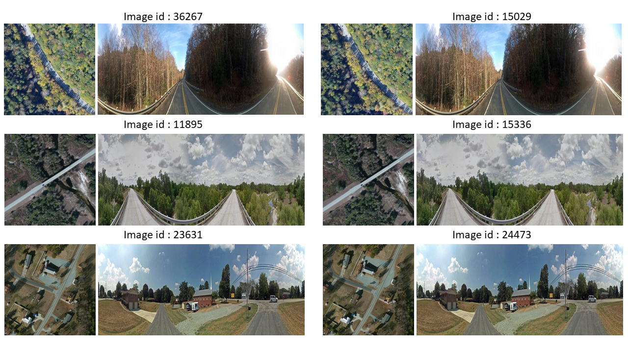
Figure 4: Three examples of repeated ground-aerial pairs from CVUSA training set.

As discussed in the main text, we identify $762$ and $43$ repeated pairs in the original training set and testing set of the CVUSA dataset, respectively. We apply the md5 algorithm on the pixel values of each image to identify these repeated pairs. We show three examples in Figure 4.

Societal Impact

Cross-view geo-localization is similar to other localization techniques such as GPS which is based on satellite or Enhanced Observed Time Difference (E-OTD) which is localized via the cellular networks that provide localization service for the users. As discussed in the main text, cross-view geo-localization can be applied in many areas such as autonomous driving, unmanned aerial vehicle navigation, and augmented reality. It can also serve as an auxiliary technique for positioning smart devices in metropolitan areas where GPS signals and mobile phone signals are usually weak due to dense buildings. It is also worth mentioning that there could be potential exposure of users’ private location information due to the nature of the localization technique. Also, there might be exposure of other information such as license plate, vehicle model, etc. However, with proposer anonymous approaches, our proposed method can benefit society in many aspects.

Implementation Details

Implementation Details

We implement our proposed model in Pytorch (Paszke et al. 2019). The ground images and aerial images are resized to $122\times 671$ and $256\times 256$, respectively. Similar to previous methods (Shi et al. 2019, 2020a; Yang, Lu, and Zhu 2021; Toker et al. 2021; Hu et al. 2018), we set the batch size to $32$ and $\alpha$ to $10$ in soft margin triplet loss. Within each batch, the exhaustive mini-batch strategy (Vo and Hays 2016) is utilized for constructing triplet pairs. We use AdamW (Loshchilov and Hutter 2017) to train our algorithm for $200$ epochs with a weight decay of $0.03$ on a single Nvidia V100 GPU. The learning rate is chosen to be $10^{-4}$ with the cosine learning rate schedule. The $\beta$ in counterfactual loss is set to $5$. The backbone ResNet34 (He et al. 2016) is pretrained on ImageNet (Deng et al. 2009). We adopt a $2$-layer transformer with $4$ heads for the geometric layout extractor which is initialized randomly. The number of geometric descriptors $K$ is set to $8$.

Semantic augmentation

We implement our semantic augmentation by using the TorchVision library. We use ColorJitter to randomly adjust brightness, contrast, and saturation. We set each parameter to $0.3$ in this function. RandomGrayscale and RandomPosterize are used for randomly applying image grayscale and image posterizing during training with a probability of $0.2$. Finally, we apply Gaussian blur with a random kernel size chosen from $\{1,3,5\}$ and a random sigma chosen within $[0.1,5]$.

Geometric Layout Extractor

As discussed in the main text, our geometric layout extractor is built on the standard transformer. In our implementation, we adopt the Pytorch official implementation of transformer . For each transformer encoder layer, we set the latent dimension to $168$, the feedforward layer dimension to $2048$, and the drop out the probability to $0.3$. We adopt layer norm and $GeLU$ activation function for each layer. At last, a $HardTanh$ activation function is applied before the output of the produced geometric layout descriptors.

Computational Efficiency

	L2LTR	Ours
# of Parameters	195.9M	48.5M
Inference Time	405ms	235ms
Pretraining	ImageNet-21K for ViT	ImageNet-1K for ResNet34 only
Computational Cost	46.77 GFLOPS	39.89 GFLOPS

Table 6: Comparison between GeoDTR and L2LTR (Yang, Lu, and Zhu 2021) on the number of parameters, inference time, initialization model, and computational cost. All experiments are conducted on a single Nvidia V100 GPU with batch size 32.

In this section, we directly compare the number of parameters, inference time, and pretrained weight between GeoDTR and current state-of-the-art methods L2LTR (Yang, Lu, and Zhu 2021). The number of parameters of GeoDTR is only $48.5M$ which is $5\times$ fewer parameters than L2LTR ($195.9M$). The inference time for GeoDTR is $235$ ms and L2LTR is $405$ ms. We almost double the inference speed compared with L2LTR. We also measure the computational cost in terms of FLOPS. Our method achieves $39.89$ GFLOPS, while L2LTR needs $46.77$ GFLOPS. Finally, GeoDTR only needs ResNet34 (He et al. 2016) pretrained model for the backbone and is randomly initialized for the other components. L2LTR is initialized with weights from ViT (Dosovitskiy et al. 2021) which is pretrained on ImageNet-21K.

More Ablation Study

In this section, we present the complete results of ablation study on different LS levels, different number of geometric layout descriptors, applying LS to other models, the effectiveness of the counterfactual process, and different transformer architectures.

Different LS levels

LS levels		Same-area				Cross-area
	Configuration	R@$1$	R@$5$	R@$10$	R@$1\%$	R@$1$	R@$5$	R@$10$	R@$1\%$
Trained on CVUSA	(none, none)	95.23%	98.71%	99.26%	99.79%	47.79%	70.52%	77.52%	92.20%
	(none, weak)	95.42%	98.01%	99.34%	99.80%	49.08%	72.46%	79.31%	92.95%
	(none, strong)	94.31%	98.41%	99.16%	99.80%	51.73%	73.75%	80.42%	93.22%
	(weak, none)	95.90%	99.00%	99.38%	99.84%	49.23%	72.17%	78.91%	92.62%
	(weak, weak)	95.86%	99.04%	99.38%	99.84%	49.47%	72.34%	79.22%	93.48%
	(weak, strong)	95.24%	98.76%	99.27%	99.84%	51.25%	73.71%	80.31%	93.57%
	(strong, none)	95.90%	99.03%	99.41%	99.84%	50.54%	74.00%	80.71%	93.10%
	(strong, weak)	96.09%	99.11%	99.43%	99.83%	53.19%	75.15%	81.13%	94.00%
	(strong, strong)	95.43%	98.86%	99.34%	99.86%	53.16%	75.62%	81.90%	93.80%
Trained on CVACT	(none, none)	87.42%	95.37%	96.50%	98.65%	29.13%	47.86%	56.21%	81.09%
	(none, weak)	87.72%	95.20%	96.29%	98.41%	32.52%	53.89%	62.88%	86.39%
	(none, strong)	86.67%	95.23%	96.35%	98.38%	42.00%	64.41%	72.32%	91.70%
	(weak, none)	86.86%	95.37%	96.69%	98.85%	29.15%	47.17%	54.78%	78.40%
	(weak, weak)	87.37%	95.84%	96.96%	98.72%	35.65%	55.81%	63.86%	85.74%
	(weak, strong)	87.04%	95.70%	96.88%	98.63%	44.63%	64.89%	72.53%	90.62%
	(strong, none)	86.75%	95.69%	96.76%	98.81%	25.71%	42.93%	50.86%	75.16%
	(strong, weak)	86.84%	95.71%	96.83%	98.76%	35.31%	55.71%	64.59%	88.01%
	(strong, strong)	86.21%	95.44%	96.72%	98.77%	44.07%	64.66%	72.08%	90.09%

Table 7: Performance of GeoDTR under different LS levels. Configurations are marked by the tuple: $(\mathcal{L}_{L},\mathcal{L}_{S})$, with $\mathcal{L}_{L},\mathcal{L}_{S}\in\{\text{none},\text{weak},\text{strong}\}$. All the models are trained with PT and CF. Results are shown for both cases when our models are trianed on CVUSA and CVACT datasets.

The experiment with different layout simulation and semantic augmentation (LS) levels (denoted as $\mathcal{L}_{L}$ and $\mathcal{L}_{S}$, respectively) is shown in Table 7. In these experiments we define three levels (none, weak, strong) for LS. “none” stands for no augmentation applied. We only apply random flip in “weak” for layout simulation. Similarly, less intensive color jitter (each parameter is set to $0.1$) and only image grayscale with a probability of $0.1$ are adopted in weak semantic augmentation. “strong” stands for applying all augmentation methods we discussed in our main paper.

Number of descriptors

# descriptors		Same-area				Cross-area
	Configuration	R@$1$	R@$5$	R@$10$	R@$1\%$	R@$1$	R@$5$	R@$10$	R@$1\%$
Trained on CVUSA	$K=1$	93.44%	98.18%	99.05%	99.80%	39.93%	63.54%	71.59%	88.92%
	$K=2$	94.09%	98.44%	99.13%	99.80%	43.07%	67.30%	74.52%	90.32%
	$K=4$	94.80%	98.64%	99.30%	99.82%	46.36%	69.37%	76.46%	91.27%
	$K=8$	95.43%	98.86%	99.34%	99.86%	53.16%	75.62%	81.90%	93.80%
Trained on CVACT	$K=1$	82.08%	94.15%	95.87%	98.63%	28.28%	46.84%	54.95%	78.56%
	$K=2$	85.00%	95.05%	96.53%	98.78%	37.72%	57.16%	65.21%	85.37%
	$K=4$	85.85%	95.50%	96.63%	98.71%	43.30%	63.90%	71.34%	88.88%
	$K=8$	86.21%	95.44%	96.72%	98.77%	44.07%	64.66%	72.08%	90.09%

Table 8: Performance of GeoDTR under different numbers of descriptors $K$. Configurations include $K=1,2,4,8$. All the models are trained with PT, LS, and CF. Results are shown for both cases when our models are trianed on CVUSA and CVACT datasets.

In Table 8, we show the full experiment results under different numbers of layout descriptors. It is observable that, increasing the number of descriptors, significantly improves the cross-area performance.

LS for other models

In Table 7, we apply LS techniques to the existing models (Yang, Lu, and Zhu 2021; Shi et al. 2019). We observe that LS bring substantial improvement on these models especially on cross-area benchmarks. This reflects the generic applicability of the proposed LS technique.

LS $+$ other methods		Same-area				Cross-area
	Configuration	R@$1$	R@$5$	R@$10$	R@$1\%$	R@$1$	R@$5$	R@$10$	R@$1\%$
Trained on CVUSA	SAFA	89.84%	96.93%	98.14%	99.64%	30.40%	52.93%	62.29%	85.82%
	SAFA w/ LS	88.19%	96.48%	98.20%	99.74%	37.15%	60.31%	69.20%	89.15%
	L2LTR	94.05%	98.27%	98.99%	99.67%	47.55%	70.58%	77.52%	91.39%
	L2LTR w/ LS	93.62%	98.46%	99.03%	99.77%	52.58%	75.81%	82.19%	93.51%
	GeoDTR w/o LS	95.23%	98.71%	99.26%	99.79%	47.79%	70.52%	77.52%	92.20%
	GeoDTR w/ LS	95.43%	98.86%	99.34%	99.86%	53.16%	75.62%	81.90%	93.80%
Trained on CVACT	SAFA	81.03%	92.80%	94.84%	98.17%	21.45%	36.55%	43.79%	69.83%
	SAFA w/ LS	79.88%	92.84%	94.71%	97.96%	25.42%	42.30%	50.36%	76.49%
	L2LTR	84.89%	94.59%	95.96%	98.37%	33.00%	51.87%	60.63%	84.79%
	L2LTR w/ LS	83.49%	94.93%	96.44%	98.68%	37.69%	57.78%	66.22%	89.63%
	GeoDTR w/o LS	87.42%	95.37%	96.50%	98.65%	29.13%	47.86%	56.21%	81.09%
	GeoDTR w/ LS	86.21%	95.44%	96.72%	98.77%	44.07%	64.66%	72.08%	90.09%

Table 9: Comparison of performance of SAFA (Shi et al. 2019), L2LTR (Yang, Lu, and Zhu 2021) and GeoDTR that are trained with or without the proposed LS technique. Our models are trained with PT and CF. Results are shown for both cases when the models are trained on CVUSA and CVACT datasets.

Counterfactual loss

The effectiveness of the proposed counterfactual (CF) learning process is demonstrated in Table 10. We conduct an ablation study of CF on models training with and without LS. We observe that, in either case, CF boosts the performance of our model on both same-area and cross-area benchmarks.

CF loss		Same-area				Cross-area
	Configuration	R@$1$	R@$5$	R@$10$	R@$1\%$	R@$1$	R@$5$	R@$10$	R@$1\%$
Trained on CVUSA	(CF, w/ LS)	95.43%	98.86%	99.34%	99.86%	53.16%	75.62%	81.90%	93.80%
	(noCF, w/ LS)	95.06%	98.72%	99.30%	99.85%	49.18%	71.96%	79.28%	92.84%
	(noCF, w/o LS)	94.83%	98.59%	99.28%	99.80%	43.71%	66.87%	74.68%	90.66%
	(CF, w/o LS)	95.23%	98.71%	99.26%	99.79%	47.79%	70.52%	77.52%	92.20%
Trained on CVACT	(8, CF, w/ LS)	86.21%	95.44%	96.72%	98.77%	44.07%	64.66%	72.08%	90.09%
	(8, noCF, w/ LS)	85.84%	95.48%	96.67%	98.71%	43.61%	64.00%	71.57%	90.04%
	(8, noCF, w/o LS)	87.01%	95.05%	96.45%	98.40%	28.26%	46.92%	55.26%	81.21%
	(8, CF, w/o LS)	87.42%	95.37%	96.50%	98.65%	29.13%	47.86%	56.21%	81.09%

Table 10: Performance of GeoDTR under different configurations, including with or without counterfactual loss (CF or noCF), and with or without LS (w/ LS or w/o LS). All the models are trained with PT. Results are shown for both cases when our model is trianed on CVUSA and CVACT datasets.

Transformer architecture

Finally, we vary the architecture of the transformer in our geometric layout extractor in Table 11. Noticeably, we observe that with increasing the number of transformer heads, the performance of our model is improved as well. Similarly, by using transformer layers it also boosts the performance. With the configuration of $4$ heads and $2$ layers, our model almost converges to a stable performance.

TR ARCH.		Same-area				Cross-area
	Configuration	R@$1$	R@$5$	R@$10$	R@$1\%$	R@$1$	R@$5$	R@$10$	R@$1\%$
Trained on CVUSA	$(8,0,0)$	92.67 %	98.19 %	99.04 %	99.78 %	46.88 %	70.81 %	78.36 %	92.99
	$(1,1,1)$	93.12%	98.19%	98.89%	99.80%	34.30%	58.89%	67.26%	87.39%
	$(1,2,1)$	93.48%	98.36%	99.09%	99.81%	41.16%	64.73%	73.18%	90.00%
	$(1,4,1)$	93.43%	98.28%	99.04%	99.76%	38.60%	62.48%	70.72%	88.90%
	$(1,4,2)$	93.44%	98.18%	99.05%	99.80%	39.93%	63.54%	71.59%	88.92%
	$(8,4,2)$	95.43%	98.86%	99.34%	99.86%	53.16%	75.62%	81.90%	93.80%
Trained on CVACT	$(8,0,0)$	83.96 %	94.29 %	96.11 %	98.60 %	37.66 %	59.57 %	67.86 %	89.69
	$(1,1,1)$	82.70%	94.50%	95.89%	98.57%	24.83%	44.63%	53.22%	80.17%
	$(1,2,1)$	83.13%	94.47%	96.22%	98.71%	25.62%	44.05%	52.78%	78.20%
	$(1,4,1)$	82.68%	94.42%	95.90%	98.63%	25.20%	43.47%	52.12%	77.27%
	$(1,4,2)$	82.08%	94.15%	95.87%	98.63%	28.28%	46.84%	54.95%	78.56%
	$(8,4,2)$	86.21%	95.44%	96.72%	98.77%	44.07%	64.66%	72.08%	90.09%

Table 11: Performance of GeoDTR under different settings of the geometric layout extractor module $\mathcal{G}^{v}(\cdot)$. Configurations are marked by the tuple: $(K,N_{h},N_{l})$ where $K$ referes to the the number of descriptors, $N_{h}$ the number of heads in the transformer encoder layer, and $N_{l}$ the number of transformer encoder layers, respectively. All the models are trained with PT, LS, and CF. Results are shown for both cases when our model is trianed on CVUSA and CVACT datasets.

Smaller latent feature dimensions

We have conducted an ablation study with a $1024$ latent feature dimension which is $4$ times less than the model we used in the main script. To achieve this goal, we replace the last convolution layer of the backbone network which outputs $512$ channels with a randomly initialized convolution layer which outputs $128$ channels before training. The same-area and cross-area performance on both CVUSA and CVACT datasets are shown in Table 12. As shown from the results, the proposed method with a smaller latent feature dimension, $\text{GeoDTR{}}_{s}$, retains the performance on the same-area experiment and only shows a small performance drop  $2\%$ on the cross-area experiment. More importantly, our model with smaller latent feature dimensions still achieves state-of-the-art performance.

Smaller feature dimension			Same-area				Cross-area
	Method	Dim	R@$1$	R@$5$	R@$10$	R@$1\%$	R@$1$	R@$5$	R@$10$	R@$1\%$
Trained on CVUSA	SAFA	4096	89.84%	96.93%	98.14%	99.64%	30.40%	52.93%	62.29%	85.82%
	L2LTR	768	94.05%	98.27%	98.99%	99.67%	47.55%	70.58%	77.52%	91.39%
	TransGeo	1024	94.08%	98.36%	99.04%	99.77%	37.18%	61.57%	69.86%	89.14%
	$\text{GeoDTR{}}_{s}$	1024	94.61%	98.57%	99.21%	99.83%	50.31%	73.34%	79.38%	92.96%
	GeoDTR	4096	95.43%	98.86%	99.34%	99.86%	53.16%	75.62%	81.90%	93.80%
Trained on CVACT	SAFA	4096	81.03%	92.80%	94.84%	98.17%	21.45%	36.55%	43.79%	69.83%
	L2LTR	768	84.89%	94.59%	95.96%	98.37%	33.00%	51.87%	60.63%	84.79%
	TransGeo	1024	84.95%	94.14%	95.78%	98.37%	17.45%	32.49%	40.48%	69.14%
	$\text{GeoDTR{}}_{s}$	1024	86.24%	95.62%	96.75%	98.59%	42.32%	62.24%	70.17%	88.62%
	GeoDTR	4096	86.21%	95.44%	96.72%	98.77%	44.07%	64.66%	72.08%	90.09%

Table 12: Comparison of our model with different latent feature dimensions with SAFA (Shi et al. 2019), L2LTR (Yang, Lu, and Zhu 2021), and TransGeo (Zhu, Shah, and Chen 2022). $\text{GeoDTR{}}_{s}$ represents the proposed model with smaller latent feature dimension. The best results are shown in magenta and the second best results are shown in blue.

More Qualitative Results

Figure 5: More visualization of geometric layout descriptors from our model trained with polar transformation on CVUSA and CVACT dataset the title stands for dataset_layout simulation_semantic augmentation.

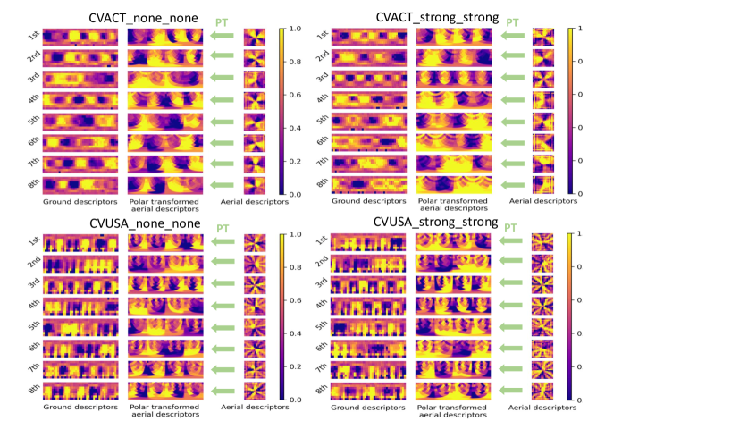
Figure 6: More visualization of geometric layout descriptors from our model trained without polar transformation on CVUSA and CVACT dataset. The naming convention is the same as in Figure 5.

More qualitative visualization of learned geometric layout descriptors are presented in Figures 5 and 6. We present models trained on different dataset and varying LS configurations. Figure 5 shows descriptors from models trained with polar transformation and Figure 6 shows descriptors from models trained without polar transformation. We can observe that the correspondence holds in different configurations of our GeoDTR on different training data.

References

- Abbasnejad et al. (2020) Abbasnejad, E.; Teney, D.; Parvaneh, A.; Shi, J.; and Hengel, A. v. d. 2020. Counterfactual Vision and Language Learning. In Proceedings of the IEEE/CVF Conference on Computer Vision and Pattern Recognition (CVPR).
- Baradel et al. (2020) Baradel, F.; Neverova, N.; Mille, J.; Mori, G.; and Wolf, C. 2020. CoPhy: Counterfactual Learning of Physical Dynamics. In International Conference on Learning Representations.
- Byrne (2019) Byrne, R. M. 2019. Counterfactuals in Explainable Artificial Intelligence (XAI): Evidence from Human Reasoning. In IJCAI, 6276–6282.
- Cai et al. (2019) Cai, S.; Guo, Y.; Khan, S.; Hu, J.; and Wen, G. 2019. Ground-to-Aerial Image Geo-Localization With a Hard Exemplar Reweighting Triplet Loss. In Proceedings of the IEEE/CVF International Conference on Computer Vision (ICCV).
- Chiu et al. (2018) Chiu, H.-P.; Murali, V.; Villamil, R.; Kessler, G. D.; Samarasekera, S.; and Kumar, R. 2018. Augmented Reality Driving Using Semantic Geo-Registration. In 2018 IEEE Conference on Virtual Reality and 3D User Interfaces (VR), 423–430.
- Deng et al. (2009) Deng, J.; Dong, W.; Socher, R.; Li, L.-J.; Li, K.; and Fei-Fei, L. 2009. ImageNet: A large-scale hierarchical image database. In 2009 IEEE Conference on Computer Vision and Pattern Recognition, 248–255.
- Dosovitskiy et al. (2021) Dosovitskiy, A.; Beyer, L.; Kolesnikov, A.; Weissenborn, D.; Zhai, X.; Unterthiner, T.; Dehghani, M.; Minderer, M.; Heigold, G.; Gelly, S.; Uszkoreit, J.; and Houlsby, N. 2021. An Image is Worth 16x16 Words: Transformers for Image Recognition at Scale. In International Conference on Learning Representations.
- Goodfellow et al. (2014) Goodfellow, I.; Pouget-Abadie, J.; Mirza, M.; Xu, B.; Warde-Farley, D.; Ozair, S.; Courville, A.; and Bengio, Y. 2014. Generative adversarial nets. Advances in neural information processing systems, 27.
- Guo et al. (2022) Guo, Y.; Choi, M.; Li, K.; Boussaid, F.; and Bennamoun, M. 2022. Soft Exemplar Highlighting for Cross-View Image-Based Geo-Localization. IEEE transactions on image processing, 31: 2094–2105.
- He et al. (2016) He, K.; Zhang, X.; Ren, S.; and Sun, J. 2016. Deep Residual Learning for Image Recognition. In Proceedings of the IEEE Conference on Computer Vision and Pattern Recognition (CVPR).
- Hu et al. (2018) Hu, S.; Feng, M.; Nguyen, R. M.; and Lee, G. H. 2018. Cvm-net: Cross-view matching network for image-based ground-to-aerial geo-localization. In Proceedings of the IEEE Conference on Computer Vision and Pattern Recognition, 7258–7267.
- Kim and Walter (2017) Kim, D.-K.; and Walter, M. R. 2017. Satellite image-based localization via learned embeddings. In 2017 IEEE International Conference on Robotics and Automation (ICRA), 2073–2080.
- Lin, Belongie, and Hays (2013) Lin, T.-Y.; Belongie, S.; and Hays, J. 2013. Cross-View Image Geolocalization. In Proceedings of the IEEE Conference on Computer Vision and Pattern Recognition (CVPR).
- Lin et al. (2015) Lin, T.-Y.; Cui, Y.; Belongie, S.; and Hays, J. 2015. Learning Deep Representations for Ground-to-Aerial Geolocalization. In Proceedings of the IEEE Conference on Computer Vision and Pattern Recognition (CVPR).
- Liu and Li (2019) Liu, L.; and Li, H. 2019. Lending Orientation to Neural Networks for Cross-View Geo-Localization. In Proceedings of the IEEE/CVF Conference on Computer Vision and Pattern Recognition (CVPR).
- Loshchilov and Hutter (2017) Loshchilov, I.; and Hutter, F. 2017. Decoupled weight decay regularization. arXiv preprint arXiv:1711.05101.
- Paszke et al. (2019) Paszke, A.; Gross, S.; Massa, F.; Lerer, A.; Bradbury, J.; Chanan, G.; Killeen, T.; Lin, Z.; Gimelshein, N.; Antiga, L.; Desmaison, A.; Kopf, A.; Yang, E.; DeVito, Z.; Raison, M.; Tejani, A.; Chilamkurthy, S.; Steiner, B.; Fang, L.; Bai, J.; and Chintala, S. 2019. PyTorch: An Imperative Style, High-Performance Deep Learning Library. In Wallach, H.; Larochelle, H.; Beygelzimer, A.; d'Alché-Buc, F.; Fox, E.; and Garnett, R., eds., Advances in Neural Information Processing Systems 32, 8024–8035. Curran Associates, Inc.
- Pearl (2009) Pearl, J. 2009. Causality: Models, Reasoning and Inference. USA: Cambridge University Press, 2nd edition. ISBN 052189560X.
- Rao et al. (2021) Rao, Y.; Chen, G.; Lu, J.; and Zhou, J. 2021. Counterfactual Attention Learning for Fine-Grained Visual Categorization and Re-Identification. In Proceedings of the IEEE/CVF International Conference on Computer Vision (ICCV), 1025–1034.
- Regmi and Shah (2019) Regmi, K.; and Shah, M. 2019. Bridging the Domain Gap for Ground-to-Aerial Image Matching. In Proceedings of the IEEE/CVF International Conference on Computer Vision (ICCV).
- Rodrigues and Tani (2021) Rodrigues, R.; and Tani, M. 2021. Are These From the Same Place? Seeing the Unseen in Cross-View Image Geo-Localization. In Proceedings of the IEEE/CVF Winter Conference on Applications of Computer Vision (WACV), 3753–3761.
- Rodrigues and Tani (2022) Rodrigues, R.; and Tani, M. 2022. Global Assists Local: Effective Aerial Representations for Field of View Constrained Image Geo-Localization. In Proceedings of the IEEE/CVF Winter Conference on Applications of Computer Vision (WACV), 3871–3879.
- Shetty and Gao (2019) Shetty, A.; and Gao, G. X. 2019. UAV Pose Estimation using Cross-view Geolocalization with Satellite Imagery. In 2019 International Conference on Robotics and Automation (ICRA), 1827–1833.
- Shi et al. (2019) Shi, Y.; Liu, L.; Yu, X.; and Li, H. 2019. Spatial-aware feature aggregation for image based cross-view geo-localization. Advances in Neural Information Processing Systems, 32: 10090–10100.
- Shi et al. (2020a) Shi, Y.; Yu, X.; Campbell, D.; and Li, H. 2020a. Where Am I Looking At? Joint Location and Orientation Estimation by Cross-View Matching. In Proceedings of the IEEE/CVF Conference on Computer Vision and Pattern Recognition (CVPR).
- Shi et al. (2020b) Shi, Y.; Yu, X.; Liu, L.; Zhang, T.; and Li, H. 2020b. Optimal Feature Transport for Cross-View Image Geo-Localization. Proceedings of the AAAI Conference on Artificial Intelligence, 34(07): 11990–11997.
- Toker et al. (2021) Toker, A.; Zhou, Q.; Maximov, M.; and Leal-Taixe, L. 2021. Coming Down to Earth: Satellite-to-Street View Synthesis for Geo-Localization. In Proceedings of the IEEE/CVF Conference on Computer Vision and Pattern Recognition (CVPR), 6488–6497.
- Vaswani et al. (2017) Vaswani, A.; Shazeer, N.; Parmar, N.; Uszkoreit, J.; Jones, L.; Gomez, A. N.; Kaiser, L. u.; and Polosukhin, I. 2017. Attention is All you Need. In Guyon, I.; Luxburg, U. V.; Bengio, S.; Wallach, H.; Fergus, R.; Vishwanathan, S.; and Garnett, R., eds., Advances in Neural Information Processing Systems, volume 30. Curran Associates, Inc.
- Vo and Hays (2016) Vo, N. N.; and Hays, J. 2016. Localizing and Orienting Street Views Using Overhead Imagery. In Leibe, B.; Matas, J.; Sebe, N.; and Welling, M., eds., Computer Vision – ECCV 2016, 494–509. Cham: Springer International Publishing. ISBN 978-3-319-46448-0.
- Wang et al. (2021) Wang, T.; Zheng, Z.; Yan, C.; Zhang, J.; Sun, Y.; Zheng, B.; and Yang, Y. 2021. Each Part Matters: Local Patterns Facilitate Cross-view Geo-localization. IEEE Transactions on Circuits and Systems for Video Technology, 1–1.
- Wang et al. (2019) Wang, Y.; Wan, Y.; Zhang, C.; Bai, L.; Cui, L.; and Yu, P. 2019. Competitive multi-agent deep reinforcement learning with counterfactual thinking. In 2019 IEEE International Conference on Data Mining (ICDM), 1366–1371. IEEE.
- Wilson et al. (2021) Wilson, D.; Zhang, X.; Sultani, W.; and Wshah, S. 2021. Visual and Object Geo-localization: A Comprehensive Survey. arXiv preprint arXiv:2112.15202.
- Workman, Souvenir, and Jacobs (2015) Workman, S.; Souvenir, R.; and Jacobs, N. 2015. Wide-Area Image Geolocalization With Aerial Reference Imagery. In Proceedings of the IEEE International Conference on Computer Vision (ICCV).
- Yang, Lu, and Zhu (2021) Yang, H.; Lu, X.; and Zhu, Y. 2021. Cross-view Geo-localization with Layer-to-Layer Transformer. In Ranzato, M.; Beygelzimer, A.; Dauphin, Y.; Liang, P.; and Vaughan, J. W., eds., Advances in Neural Information Processing Systems, volume 34, 29009–29020. Curran Associates, Inc.
- Zheng, Wei, and Yang (2020) Zheng, Z.; Wei, Y.; and Yang, Y. 2020. University-1652: A Multi-View Multi-Source Benchmark for Drone-Based Geo-Localization. In Proceedings of the 28th ACM International Conference on Multimedia, MM ’20, 1395–1403. New York, NY, USA: Association for Computing Machinery. ISBN 9781450379885.
- Zhu, Shah, and Chen (2022) Zhu, S.; Shah, M.; and Chen, C. 2022. TransGeo: Transformer Is All You Need for Cross-View Image Geo-Localization. In Proceedings of the IEEE/CVF Conference on Computer Vision and Pattern Recognition (CVPR), 1162–1171.