Fractionally integrated curve time series with cointegration

Abstract

We introduce methods and theory for fractionally cointegrated curve time series. We develop a variance ratio test to determine the dimensions associated with the nonstationary and stationary subspaces. For each subspace, we apply a local Whittle estimator to estimate the long-memory parameter and establish its consistency. A Monte Carlo study of finite-sample performance is included, along with an empirical application.

JEL codes: C12; C14; C32

MSC 2010: 37M10; 62F03

Keywords: fractional cointegration; long memory time series; functional data; functional principal component analysis; limit theorems.

1 Introduction

Functional time series analysis is a harmony between functional data and time series analyses. Similar to univariate and multivariate time series, there exists a temporal dependence structure in functional observations. For example, intraday volatility functions are serially dependent and often exhibit long-memory feature (Lobato97). Time series of airway pressure are used for monitoring patients undergoing mechanical ventilation, such series exhibits periodically strong dependence (BNF+23).

In functional time series analysis, the bulk of literature assuming stationarity over the short-range temporal dependence (see, e.g., Bosq2000; FV06; BYZ10; Hoermann2010; Horvath2012; Horvath2014; Laurini2014; Klepsch2017a). Only in recent years, there has been some development on long-memory functional time series models (see, e.g., Li2020a; Li2021; Li2020; RP20). The long-memory functional time series describes processes with greater persistence than short-range dependent ones, such that in the stationary case autocovariances decay very slowly and the spectral density is unbounded, especially at frequency zero. While Li2020a; Li2021 consider inference and estimation of long-memory parameter in stationary curve time series, Li2020 studies inferential results for nonstationary curve time series. Based on the mean squared error, Shang20 and Shang22 evaluate and compare various long-memory parameter estimators for stationary and nonstationary curve time series, respectively. In these comparisons, the local Whittle estimator of robinson1995gaussian is recommended. While Li2021 presents the asymptotic properties of the local Whittle estimator, Shang22b applies a sieve bootstrap method of Paparoditis18 to nonparametrically construct the confidence intervals of the memory parameter.

Given the recent surge of interest in functional time series analysis, cointegration methods have been extended to a functional time series setting by Chang2016. They define cointegration for curve time series and develop statistical methods based on functional principal component analysis. Beare2017b and Seo2019 extend the Granger-Johansen representation theorem to a Hilbert space and a Bayes Hilbert space, respectively. While Beare2017b provide a representation of I(1) autoregressive Hilbertian process, Beare2020 present a representation of I(1) and I(2) autoregressive Hilbertian processes; see also Franchi2020 and Seo2022 for similar representation results in a more general setting.

We study a fractionally cointegrated curve time series by developing inferential and estimation methods for such a time series. The curve time series consists of nonstationary and stationary components. For each component, we estimate the long-memory parameter via the local Whittle estimator. Through a variance ratio test, we determine the subspaces spanned by nonstationary and stationary components. We compare the selected subspaces with the modified eigen-value ratio estimator of Li2020a. In addition, this paper also develops statistical methods for the case when the stationary component can further be decomposed into the long-memory and short-memory components.

In Section 2, we present our notations and preliminaries. In Section 3, we introduce the fractionally cointegrated functional time series. The estimation procedure is given in Section 4. Illustrated by a series of simulation studies in Section 5, we evaluate the estimation accuracy of the proposed method and compare the result with the one by Li2020. The empirical performance of our proposed method is also validated through a Swedish human mortality data set in Section 5.2. In Section LABEL:sec:conclude, we conclude and present some idea on how the methodology can be further extended.

2 Preliminaries

In the subsequent discussion, we assume that the curve-valued time series $Z_{t}$ of interest takes values in the Hilbert space $\mathcal{H}$ of square-integrable functions defined on $[0,1]$. We let $\langle h_{1},h_{2}\rangle$ denote the inner product of $h_{1},h_{2}\in\mathcal{H}$, and then let $\|h\|$ denote the norm of $h\in\mathcal{H}$, which is defined by $\langle h,h\rangle^{1/2}$. Given a set $G\subseteq\mathcal{H}$, we let $G^{\perp}$ denote the orthogonal complement to $G$. We denote by $\mathcal{L}_{\mathcal{H}}$ the space of bounded linear operators acting on $\mathcal{H}$ equipped with the uniform norm $\|A\|_{\mathcal{L}_{\mathcal{H}}}=\sup_{\|h\|\leq 1}\|Ah\|$. The adjoint $A^{\ast}$ of a linear operator $A\in\mathcal{L}_{\mathcal{H}}$ is the unique linear operator satisfying $\langle Ah_{1},h_{2}\rangle=\langle h_{1},A^{\ast}h_{2}\rangle$ for all $h_{1},h_{2}\in\mathcal{H}$. We will say that an operator $A\in\mathcal{L}_{\mathcal{H}}$ is nonnegative (resp. positive) definite if $\langle Ah,h\rangle\geq 0$ (resp. $\langle Ah,h\rangle>0$) for all nonzero $h\in\mathcal{H}$. We let $\otimes$ denote the tensor product of elements in $\mathcal{H}$, i.e., $h_{1}\otimes h_{2}$ denotes the linear map given by $\langle h_{1},\cdot\rangle h_{2}$ for any $h_{1},h_{2}\in\mathcal{H}$. We let the range of $A\in\mathcal{L}_{\mathcal{H}}$ be denoted by $\operatorname{ran}A$. The dimension of $\operatorname{ran}A$ is called the rank of $A$, denoted by $\operatorname{rank}A$. We will consider convergence of a sequence of random bounded linear operators as the sample size $T$ tends to infinity. For such a sequence of operators $A_{j}$, we write $A_{j}\underset{p}{\rightarrow}A$ if $\|A_{j}-A\|_{\mathcal{L}_{\mathcal{H}}}\underset{p}{\rightarrow}0$.

We define the I$(d)$ property of a time series, taking values in $\mathcal{H}$. As a crucial building block, we first introduce the I$(0)$ property adopted from Beare2017b.

Definition 1 (I$(0)$-ness).

The time series $X_{t}$ taking values in $\mathcal{H}$ is said to be I$(0)$, and denoted $X_{t}\in$ I$(0)$, if (i) it allows the representation $$X_{t}=\sum_{j=0}^{\infty}\psi_{j}\varepsilon_{t-j},$$ where $\psi_{j}\in\mathcal{L}_{\mathcal{H}}$ for all $j$ and $\varepsilon_{t}$ is an i.i.d. sequence with $\mathbb{E}X_{t}=0$ and positive definite covariance $C_{\varepsilon}:=\mathbb{E}[X_{t}\otimes X_{t}]$, and (ii) $\sum_{j=0}^{\infty}\psi_{j}$is a nonzero element in $\mathcal{L}_{\mathcal{H}}$.

The I$(0)$ time series is necessarily stationary, and its long-run covariance $\sum_{s=1}^{\infty}\sum_{t=1}^{\infty}\mathbb{E}[X_{s}\otimes X_{t}]$ is a well defined bounded linear operator (see, e.g., Beare2017b). Based on the I$(0)$ property, we define $\mathcal{H}$-valued I$(d)$ processes, which will subsequently be considered as follows:

Definition 2 (I$(d)$-ness).

For $d\geq 0$, the time series $Y_{t}$ is said to be I$(d)$ (or equivalently, fractionally integrated of order $d$), and denoted $Y_{t}\in$ I$(d)$, if $\Delta^{d}Y_{t}$ can be made I$(0)$ for some relevant past values of $\Delta^{d}Y_{t}$, where $\Delta^{d}$ is a power series of the lag operator defined by

$$\Delta^{d}=\sum_{j=0}^{\infty}\frac{\Gamma(j-d)}{\Gamma(-d)\Gamma(j+1)}L^{j}.$$

Note that in the above definition of the I$(d)$ property, we do not require $\Delta^{d}Y_{t}$ to be exactly I$(0)$ but require the existence of relevant past values that can make the time series of $\Delta^{d}Y_{t}$ be I$(0)$. This is a necessary mathematical treatment since we will consider the nonstationary case with $d>1/2$ in the subsequent discussion.

Cointegration is the property of multivariate nonstationary time series, implying the existence of a stationary linear combination. A cointegrating relationship of a collection of nonstationary variables is oftentimes understood as their stable long-run relationship. This notion has been extended to and studied in a Hilbert space setting by Beare2017b, Li2020, Nielsen2019, and Seo2022; Seo2020. Extending these former notions of cointegration, we may define fractional cointegration in $\mathcal{H}$ as follows:

Definition 3 (Fractional cointegration).

Suppose that $Y_{t}\in$ I$(d)$, $\langle Y_{t},v\rangle\in$ I$(d-b)$ for some $d\geq 1/2$, $b\in(d-1/2,d]$ and $v\in\mathcal{H}$. We then say that $Y_{t}$ is (fractionally) cointegrated in the direction of $v$ and call $v$ a (fractional) cointegrating vector.

If $d\geq 1/2$, an I$(d)$ time series $Y_{t}$ taking values in $\mathcal{H}$ is nonstationary. However, given that (i) an inner product with some element of $v$ can represent any arbitrary bounded linear functional defined on $\mathcal{H}$ (the Riesz representation theorem) and (ii) the time series $\langle Y_{t},{v}\rangle$ is I$(d-b)$ for $d-b<1/2$ and thus can be made stationary for some past values of $\langle Y_{t},{v}\rangle$, the transformation $x\mapsto\langle x,v\rangle$ is exactly like the cointegrating vector considered in Euclidean space setting.

3 Fractionally cointegrated functional time series

We consider modeling nonstationary dependent curve-valued observations but exhibiting stable long-run linear relationships as fractionally cointegrated time series. A potential example of such a time series may be yield curves over time; it turns out that this time series tends to evolve like a nonstationary process (Li2020), but due to the expectation hypothesis, many linear functionals of such time series are expected not to exhibit nonstationarity.

Even if Definition 3 gives us a proper notion of $\mathcal{H}$-valued time series allowing fractional cointegration, the definition itself is, of course, not sufficient for the inferential methods to be developed. For statistical analysis, we employ the following assumptions for the observed time series $Z_{t}$: below, $\Delta^{d}_{+}$ denotes the truncated fractional difference operator defined by $\Delta^{-d}_{+}X_{t}=\Delta^{-d}X_{t}\mathds{1}\{t\geq 1\}$, i.e.,

$$\Delta^{d}_{+}=\sum_{j=0}^{t-1}\frac{\Gamma(j-d)}{\Gamma(-d)\Gamma(j+1)}L^{j}.$$

Assumption 1.

The observed time series $Z_{t}$, taking values in $\mathcal{H}$, satisfies the following:

1. $Z_{t}=\mu+Y_{t}$ for some $\mu\in\mathcal{H}$.

2. For some $d\in(1/2,3/2)$, $b>0$ with $0\leq d-b<1/2$, there exists an orthogonal projection $P$ and an I(0) sequence $X_{t}$ given by $X_{t}=\sum_{j=0}^{\infty}\psi_{j}\varepsilon_{t-j}$ satisfying

   $$P(Y_{t}-Y_{0}) =\Delta^{-d}_{+}PX_{t},$$ (3.1)

   $$(I-P)Y_{t} =\Delta^{-(d-b)}(I-P)X_{t}=\sum_{j=0}^{\infty}b_{j}\varepsilon_{t-j},$$ (3.2)

   where $b_{j}=\sum_{k=0}^{\infty}\frac{\Gamma(j-k+d)}{\Gamma(d)\Gamma(j-k+1)}(I-P)\psi_{j}$, $\sum_{j=0}^{\infty}j\|\psi_{j}\|^{2}<\infty$, and $\varepsilon_{t}$ satisfies that $\mathbb{E}\|\varepsilon_{t}\|^{\tau}<\infty$ for some $\tau>\max\{4,2/(2d-1)\}$.

3. $\operatorname{rank}P\sum_{j=0}^{\infty}\psi_{j}=q_{d}<\infty$.

Some comments on Assumption 1 are in order. First, in most empirical applications, a functional time series tends to have a nonzero intercept. Thus, in a, we assume that the observed time series is given by the sum of an I$(d)$ process $Y_{t}$ and an unobserved intercept $\mu\in\mathcal{H}$. Moreover, of course, it might sometimes be of interest to consider a linear time trend component; even if we do not explicitly deal with this case, most of the results to be subsequently given may be extended to accommodate this possibility with moderate modifications. We describe the cointegrating properties of the stochastic part of the observed time series $Z_{t}$ in b with some other necessary conditions for our mathematical development. Here we restrict our interest to the case with $d\in(1/2,3/2)$, which seems relevant in most empirical applications involving nonstationary fractional integrated time series.

Note also that we require $(I-P)Y_{t}$ to be a stationary long-range dependent (LRD) process. Given that any orthogonal projection may be understood as a bipartite decomposition of a Hilbert space, what 3.1 and 3.2 imply is that our observed time series may be understood as the sum of two heterogeneous components: the nonstationary component $P(Y_{t}-Y_{0})$ and the stationary component $(I-P)Y_{t}$. Associated with this condition, c identifies the collection of the cointegrating vectors as $\operatorname{ran}(I-P)$; under this condition, $\langle Y_{t},v\rangle$ is a stationary LRD process if and only if $v\in\operatorname{ran}(I-P)$.

However, given that (i) our I$(0)$ property does not require $\langle X_{t},v\rangle$ to be I$(0)$ for all $v\in\mathcal{H}$ and (ii) $\operatorname{ran}(I-P)\sum_{j=0}^{\infty}\psi_{j}$may not be equal to $\operatorname{ran}(I-P)$, c does not imply that $\langle Y_{t},v\rangle$ needs to be I$(d-b)$ for any $v\in\operatorname{ran}(I-P)$, but allows $\langle Y_{t},v\rangle$ to be integrated of any arbitrary order $d_{\ell}\in[0,d-b]$. That is, the time series $(I-P)Y_{t}$ is a quite general stationary process. Given this time series, we are interested in identifying the nonstationary and stationary components from the observed time series, which will be discussed in the next section.

Sometimes, practitioners may also be interested in the case where the stationary part of $Y_{t}$ can be decomposed into the short-range dependent (SRD) and LRD components. We will also consider this case by imposing the following additional conditions on the stationary component:

Assumption 1A.

The observed time series $Z_{t}$ satisfies Assumption 1, and there exists an orthogonal projection $Q$ such that

$$Q(I-P)Y_{t} =\Delta^{-(d-b)}Q(I-P)X_{t},$$

$$(I-Q)(I-P)Y_{t} =(I-Q)(I-P)X_{t},$$

and

$$\operatorname{rank}Q(I-P)\sum_{j=0}^{\infty}\psi_{j}=q_{d-b}<\infty.$$

Under Assumption 1A, the time series $\{Z_{t}\}_{t\geq 1}$ satisfying Assumption 1 can be decomposed into three different components: $q_{d}-$dimensional nonstationary, $q_{d-b}-$dimensional LRD and infinite-dimensional SRD components. In this case, practitioners may be interested in decomposing the nonstationary component from the stationary component (given by the sum of the LRD and SRD components) and in decomposing the LRD component from the SRD component. Moreover, the memory parameters $d$ and $d-b$ may also be useful in practice. We will also discuss these issues.

It will be convenient to introduce some additional notation and terminology. Under Assumption 1, we have the bipartite decomposition $\mathcal{H}=\operatorname{ran}P\oplus\operatorname{ran}(I-P)$. As clarified above, the collection of cointegrating vectors is given by $\operatorname{ran}(I-P)$, which is called the cointegrating space and denoted by $\mathcal{H}_{S}$. The orthogonal complement to $\mathcal{H}_{S}$ is called the dominant subspace (as in Li2020) and denoted by $\mathcal{H}_{N}$. If Assumption 1A is satisfied, then $\mathcal{H}_{S}$ can also be decomposed into $Q\mathcal{H}_{S}$ and $(I-Q)\mathcal{H}_{S}$, which are called the LRD and SRD subspaces and denoted by $\mathcal{H}_{LRD}$ and $\mathcal{H}_{SRD}$. To sum up, we have

$$\mathcal{H} =\mathcal{H}_{N}\oplus\mathcal{H}_{S}\quad\hskip 57.81621pt\text{under Assumption~{}\ref{assum1}},$$

$$\mathcal{H} =\mathcal{H}_{N}\oplus\mathcal{H}_{LRD}\oplus H_{SRD}\quad\text{under Assumption~{}\ref{assum2add}}.$$

4 Statistical methods

To make our statistical inference invariant with respect to (possibly) nonzero intercept $\mu$, we will consider $Z_{t}^{0}$ or $\overline{Z}_{t}$ depending on the context, which is defined as follows: for $t\geq 1$,

$$Z_{t}^{0}=Z_{t}-Z_{0}\quad\text{and}\quad\overline{Z}_{t}=Z_{t}-\frac{1}{T}\sum_{t=1}^{T}Z_{t},$$ (4.1)

where we assume that $Z_{0}$ is observed. Of course, in practice, $Z_{t}^{0}$ will be replaced by $Z_{t}-Z_{1}$ by putting the first observation aside to initialize the time series. Thus, no essential restriction is placed by using $Z_{t}^{0}$ in analysis.

4.1 Decomposition of $\mathcal{H}_{N}$ and $\mathcal{H}_{S}$

In this section, we consider the decomposition of the nonstationary and stationary components, which essentially boils down to identifying the cointegrating space $\mathcal{H}_{S}$ or the dominant subspace $\mathcal{H}_{N}$. As may be deduced from the existing literature (see, e.g., Chang2016; Nielsen2019; Li2020), the dominant subspace $\mathcal{H}_{N}$ can be estimated by the span of the eigenvectors corresponding to the first $q_{d}$ largest eigenvalues of a certain sample operator. For this reason, the estimation of $\mathcal{H}_{S}$ reduces to the estimation of $q_{d}$, which will be subsequently discussed. The quantity $q_{d}$ itself may be of interest to practitioners since it represents the number of linearly independent fractional unit root processes embedded into the time series; in the literature considering $n$-dimensional vector-valued fractionally integrated time series, the quantity $n-q_{d}$ is commonly called the (fractional) cointegrating rank and has been paid lots of attention. We will develop statistical inference on $q_{d}$ in this section and obtain the desired decomposition.

4.1.1 Eigenvalue-ratio-based estimation of $q_{d}$

We will first consider an eigenvalue-ratio-based estimator, similar to Li2020 estimator of the dimension of the dominant subspace. This estimator will perform worse in finite samples than our second estimator obtained by the proposed sequential testing procedure in finite samples. Nevertheless, the subsequent discussion becomes a crucial input to the aforementioned testing procedure and helps a deeper understanding of fractionally cointegrated time series.

Under Assumption 1, an element $v$ included in the dominant subspace $\mathcal{H}_{N}$ is differentiated with any other element $\widetilde{v}\in\mathcal{H}_{S}$ in the sense that the sample variance of $\langle Y_{t},v\rangle$ tends to be higher than that of $\langle Y_{t},\widetilde{v}\rangle$; more specifically, we have

$$\frac{T^{-1}\sum_{t=1}^{T}\langle Y_{t},v\rangle^{2}}{T^{-1}\sum_{t=1}^{T}\langle Y_{t},\widetilde{v}\rangle^{2}}\underset{p}{\rightarrow}0.$$

Based on the above intuition combined with Lemma LABEL:lemwkc and the asymptotic properties of the covariance operator of nonstationary fractionally integrated functional time series, we may establish the following result:

Proposition 4.1.

Suppose that Assumption 1 holds, $K$ is a finite integer satisfying $K>q_{d}$ and the $(K-q_{d})$-th largest eigenvalue of $\mathbb{E}[(I-P)Y_{t}\otimes(I-P)Y_{t}]$ is nonzero and distinct from the next one. Let $(\widehat{\mu}_{1},\ldots,\widehat{\mu}_{K})$ be the ordered (from the largest) eigenvalues of the sample covariance operator of $Z_{t}$ given by

$$\widehat{C}_{\overline{Z}}=\frac{1}{T}\sum_{t=1}^{T}\overline{Z_{t}}\otimes\overline{Z}_{t}.$$

Then the following holds:

1. ${\widehat{\mu}_{j}}/{\widehat{\mu}_{j+1}}\underset{p}{\rightarrow}\infty$ if $j=q_{d}$ while ${\widehat{\mu}_{j}}/{\widehat{\mu}_{j+1}}=O_{p}(1)$ if $j\neq q_{d}$.

2. The corresponding eigenvectors $(\widehat{v}_{1},\ldots,\widehat{v}_{q_{d}})$ satisfy that

   $$\sum_{j=1}^{{q}_{d}}\widehat{v}_{j}\otimes\widehat{v}_{j}\underset{p}{\rightarrow}P.$$ (4.2)

Some direct consequences of the results given in Proposition 4.1 are given as follows:

Corollary 4.1.

Let everything be as in Proposition 4.1. Then the following hold.

1. $\widehat{q}_{d}:=\operatornamewithlimits{argmax}_{1\leq j\leq K}\left(\frac{\widehat{\mu}_{j}}{\widehat{\mu}_{j+1}}\right)\underset{p}{\rightarrow}q_{d}$.

2. $\widehat{P}:=\sum_{j=1}^{\widehat{q}_{d}}\widehat{v}_{j}\otimes\widehat{v}_{j}\underset{p}{\rightarrow}P$.

Note that Proposition 4.1 requires a careful choice of $K$ satisfying some mathematical conditions, which is crucial to have the consistency results given in Corollary 4.1 (see Remark 4.1). However, such a choice can be obtained feasibly without difficulty (see Remark 4.3). It is also worth emphasizing that our results given in Proposition 4.1 and Corollary 4.1 require only that the $(K-q_{d})$-th eigenvalue of $\mathbb{E}[(I-P)Y_{t}\otimes(I-P)Y_{t}]$ is different from the next one; this allows the case where some of the first $(K-q_{d})$ eigenvalues are tied and does not seem to be a restrictive assumption in practice. Given that any closed subspace of $\mathcal{H}$ may be identified as the unique orthogonal projection onto the space, ii in Corollary 4.1 may be understood as the convergence of $\operatorname{ran}\widehat{P}$ (resp. $\operatorname{ran}(I-\widehat{P})$) to $\mathcal{H}_{N}$ (resp. $\mathcal{H}_{S}$), we thus may write

$$\operatorname{ran}\widehat{P}\underset{p}{\rightarrow}\mathcal{H}_{N}\quad\text{and}\quad\operatorname{ran}(I-\widehat{P})\underset{p}{\rightarrow}\mathcal{H}_{S}.$$

Remark 4.1.

In our proof of Proposition 4.1, it is shown that, for some $\Omega$ which is symmetric and positive definite on $\mathcal{H}_{N}$,

$$T^{1-2d}\widehat{\mu}_{j} \underset{d}{\rightarrow}\text{$j$-th largest eigenvalue of }\int_{0}^{1}\Omega\overline{W}_{d}(s)\otimes\Omega\overline{W}_{d}(s)ds,\quad\text{jointly for $j\leq q_{d}$},$$

$$\widehat{\mu}_{j} \underset{p}{\rightarrow}\text{$j$-th largest eigenvalue of }\mathbb{E}[(I-P){Y}_{t}\otimes(I-P){Y}_{t}],\quad\text{jointly for $j>q_{d}$},$$ (4.3)

where, as will be introduced in Section LABEL:sec_appen, $\overline{W}_{d}$ is a demeaned Type II fractional Brownian motion of order $d$ defined on $\mathcal{H}_{N}$. The results given in Proposition 4.1i are consequences of the above convergence results. Moreover, this shows why we require the $(K-q_{d})$-th eigenvalue of $\mathbb{E}[(I-P)Y_{t}\otimes(I-P)Y_{t}]$ to be nonzero in Proposition 4.1; if the $(K-q_{d})$-th eigenvalue is zero, then $\widehat{\mu}_{K-1}/\widehat{\mu}_{K}\underset{p}{\rightarrow}\infty$ which is not desirable for consistency of $\widehat{q}_{d}$.

Remark 4.2.

The estimator given in Proposition 4.1 may be understood as a tailored version of Li2020 eigenvalue-ratio estimator of the dimension of the dominant subspace. It is worth noting two important differences in theoretical and practical aspects. First, due to cointegration, we can explain more about the role of $K$ (an upper bound of $q_{d}$, which needs to be chosen by a researcher) while its role is not sufficiently discovered in Li2020 setting. Due to this, Li2020 estimator requires an additional and arbitrary penalty parameter to suppress the possibility that two small eigenvalues result in a large ratio and hence may give a misleading estimate. On the other hand, we can provide a feasible and less arbitrary way to choose $K$ (see Remark 4.3 below).

Remark 4.3.

In Proposition 4.1, $K$ needs to be greater than $q_{d}$. We know from Remark 4.1 that the first $q_{d}$ largest eigenvalues of $\widehat{C}_{\overline{Z}}$ have bigger stochastic orders than the remaining eigenvalues. It thus may not be difficult to conjecture a slightly bigger integer than $q_{d}$ from the estimated eigenvalues, and $K$ can be set to such an integer. Note that we also require the $(K-q_{d})$-th eigenvalue of $\mathbb{E}[(I-P)Y_{t}\otimes(I-P)Y_{t}]$ to be nonzero and distinct from the next one. Given that we consider a functional time series of which dimension is very high, $\mathbb{E}[(I-P)Y_{t}\otimes(I-P)Y_{t}]$ tends to allow many nonzero eigenvalues in most empirical applications. Moreover, violation of this condition may be avoided by checking if $\widehat{\mu}_{K}-\widehat{\mu}_{K+1}$ is bounded away from zero (see 4.3).

Even if we can consistently estimate $q_{d}$ (and thus $P$) based on Proposition 4.1, practitioners may be more interested in a statistical test for $q_{d}$, which provides how strongly the data support a certain hypothesis about $q_{d}$. In the next section, we provide a variance-ratio-type test for $q_{d}$ that can be applied to our functional time series setting and propose an alternative estimator $\overline{q}_{d}$ obtained by sequential application of the test. Our simulation results show that this new estimator tends to outperform $\widehat{q}_{d}$.

4.1.2 Variance-ratio test of $q_{d}$

The limiting behavior of the sample covariance operator $\widehat{C}_{\overline{Z}}=T^{-1}\sum_{t=1}^{T}\overline{Z}_{t}\otimes\overline{Z}_{t}$ under the existence of cointegration enables us to implement a statistical test about $q_{d}$, which will be discussed in this section.

As the first step to developing our test, we consider a fractionally integrated variable $\widetilde{Z}_{t}$ as follows:

$$\widetilde{Z}_{t}=\Delta_{+}^{-\alpha}\overline{Z}_{t}.$$ (4.4)

For any positive integer $K$, let $\widehat{P}_{K}$ denote the orthogonal projection given by

$$\widehat{P}_{K}=\sum_{j=1}^{K}\widehat{v}_{j}\otimes\widehat{v}_{j},$$ (4.5)

where $(\widehat{v}_{1},\ldots,\widehat{v}_{K})$ is the eigenvectors corresponding to the first $K$ largest eigenvalues of $\widehat{C}_{\overline{Z}}$. Let $A_{T}$ and $B_{T}$ be defined by

$$A_{T}=\sum_{t=1}^{T}\widehat{P}_{K}\overline{Z}_{t}\otimes\widehat{P}_{K}\overline{Z}_{t},\quad B_{T}=\sum_{t=1}^{T}\widehat{P}_{K}\widetilde{Z}_{t}\otimes\widehat{P}_{K}\widetilde{Z}_{t}.$$

We then define the following generalized eigenvalue problem:

$$\widehat{\nu}_{j}B_{T}\widehat{w}_{j}=A_{T}\widehat{w}_{j},\quad\widehat{\nu}_{1}\leq\widehat{\nu}_{2}\leq\ldots\leq\widehat{\nu}_{K},\quad\widehat{w}_{j}\in\operatorname{ran}\widehat{P}_{K}.$$ (4.6)

Since the domain and the codomain of each of $A_{T}$ and $B_{T}$ are restricted to the span of the first $K$ eigenvectors of $\widehat{C}_{\overline{Z}}$, we may compute $K$ (almost surely) positive eigenvalues from 4.6. Our main result in this section is given as follows: in the proposition below, $B_{\delta}(s)$ denotes $q_{d}$-dimensional type II fractional standard Brownian motion defined by $B_{\delta}(0)=0$ almost surely and $B_{\delta}(s)=\frac{1}{\Gamma(\delta)}\int_{0}^{s}(s-r)^{\delta-1}dW_{0}(r)$ for $s>0$ and the standard Brownian motion $W_{0}$.

Proposition 4.2.

Suppose that Assumption 1 holds, $K$ is a finite integer satisfying $K>q_{d}$ and the $(K-q_{d})$-th largest eigenvalue of $\mathbb{E}[(I-P)Y_{t}\otimes(I-P)Y_{t}]$ is nonzero and distinct from the next one, and $\alpha>0$. Let $(\nu_{1},\ldots,\nu_{q_{d}})$ be the ordered eigenvalues (from the smallest) of

$$\left(\int_{0}^{1}\widetilde{B}_{d+\alpha}(s)\widetilde{B}_{d+\alpha}(s)^{\prime}ds\right)^{-1}\int_{0}^{1}\overline{B}_{d}(s)\overline{B}_{d}(s)^{\prime}ds,$$ (4.7)

where

$$\overline{B}_{d}(r) =B_{d}(r)-\int_{0}^{1}B_{d}(s)ds,$$

$$\widetilde{B}_{d+\alpha}(r) =B_{d+\alpha}(r)-\left(\int_{0}^{1}B_{d+\alpha}(s)ds\right)\left(\int_{0}^{r}\frac{(r-s)^{\alpha-1}}{\Gamma(\alpha)}ds\right).$$

Then

$$T^{2\alpha}(\widehat{\nu}_{1},\ldots,\widehat{\nu}_{q_{d}})\underset{d}{\rightarrow}(\nu_{1},\ldots,\nu_{q_{d}})$$

and

$$T^{2\alpha}\widehat{\nu}_{q_{d}+j}\underset{p}{\rightarrow}\infty,\quad j=1,\ldots,K-q_{d}.$$

The asymptotic results given in Proposition 4.2 enable us to implement a more detailed statistical inference on $q_{d}$ beyond consistent estimation of it. Specifically, let us consider the following null and alternative hypotheses:

$$H_{0}:q_{d}=q\quad\text{v.s.}\quad H_{1}:q_{d}<q.$$ (4.8)

Based on the asymptotic results given in Proposition 4.2, we know that, for example,

$$\Lambda_{q,\alpha}^{0}=T^{2\alpha}\max_{1\leq j\leq q}\widehat{\nu}_{j}\quad\text{and}\quad\Lambda_{q,\alpha}^{1}=T^{2\alpha}\sum_{j=1}^{q}\widehat{\nu}_{j}$$ (4.9)

have well-defined limiting distributions under $H_{0}$ while they diverge to infinity under $H_{1}$. Using these statistics, we may easily evaluate the plausibility of the null hypothesis. Moreover, as an alternative way to estimate $q_{d}$, we may sequentially examine 4.8 for $q=q_{\max},q_{\max}-1,\ldots,1$, where $q_{\max}$ is a reasonable upper bound. In practice, $q_{\max}$ may be chosen based on the estimated eigenvalues of $\widehat{C}_{\overline{Z}}$ (see Remark 4.3) or can be set to $\widehat{q}_{d}+\epsilon$ using the modified eigenvalue ratio estimator of Li2020 and small finite integer $\epsilon$. This sequential procedure is consistent in the following sense:

Corollary 4.2.

Suppose that the assumptions in Proposition 4.2 hold, and let $\overline{q}_{d}$ be the estimator obtained from this sequential procedure with fixed significance level $\eta>0$. Then,

$$\mathbb{P}(\overline{q}_{d}=q_{d})\to 1-\eta\cdot\mathds{1}\{q_{d}\geq 1\}.$$

By letting $\eta\to 0$ as $T\to\infty$, we have $\mathbb{P}(\overline{q}_{d}=q_{d})\to 1$ for all possible values of $q_{d}$.

Our proof of Proposition 4.2 also shows that the first $q_{d}$ eigenvectors computed from 4.6 converge to a random orthonormal basis of $\mathcal{H}_{N}$. Therefore, we can also obtain the following:

Corollary 4.3.

Suppose that the assumptions in Proposition 4.2 hold and let $\widetilde{q}_{d}\underset{p}{\rightarrow}q_{d}$ as $T\to\infty$. Then,

$$\widetilde{P}=\sum_{j=1}^{\widetilde{q}_{d}}\widehat{w}_{j}\otimes\widehat{w}_{j}\underset{p}{\rightarrow}P.$$

Suppose that practitioners are only interested in consistent estimation of $\mathcal{H}_{N}$ or $\mathcal{H}_{S}$; they then might prefer to use the eigenvalue-ratio estimator $\widehat{q}_{d}$ developed in Section 4.1.1 since it is much easier to implement. However, our simulation study shows that $\overline{q}_{d}$ substantially outperforms $\widehat{q}_{d}$. Since the estimation of $\mathcal{H}_{N}$ (or $\mathcal{H}_{S}$) can be affected by inaccuracy in the estimator of its dimension, this result suggests the use of the testing procedure given in Corollary 4.2 in practice.

Remark 4.4.

The limiting distribution given in Proposition 4.2 depends on $\alpha$ and $d$. Note that $d$ is an unknown parameter of interest. Therefore, in implementing the proposed test in practice, $d$ needs to be replaced by a consistent estimator of $d$, such as the local Whittle estimator that we will consider later in Section 4.3. On the other hand, $\alpha$ is known and needs to be chosen by the researcher. Our simulation results show that the test with $\alpha=0.5$ performs quite reasonably.

Remark 4.5.

If we consider a finite-dimensional Euclidean space setting, our test based on $\Lambda_{q,\alpha}^{1}$ reduces to the test of Nielsen2010 developed for fractionally cointegrated time series. Even if there are some moderate differences in the cointegrating properties assumed in the present paper and that of Nielsen2010 (e.g., in that paper, the considered time series is written as the sum of the nonstationary and asymptotically stationary components), our tests developed in this section may be viewed as generalizations of Nielsen2010 test to some degree.

4.2 Decomposition of $\mathcal{H}_{LRD}$ and $\mathcal{H}_{SRD}$

We, in this section, consider the estimation of $\mathcal{H}_{LRD}$ and $\mathcal{H}_{SRD}$ in the case where $\mathcal{H}_{S}$ can be further decomposed as in Assumption 1A; of course, this requires a consistent estimator of $\mathcal{H}_{S}$ in advance. The variance-ratio test developed in Section 4.1.2 cannot be directly used to this problem since it requires nonstationarity of the underlying time series. As an alternative method, we here provide a consistent estimator of $q_{d-b}$, similar to the eigenvalue-ratio estimator considered in Section 4.1.1.

Suppose that $P$ is known. We then know that the long-run variance of $\langle Y_{t},v\rangle$ for $v\in\mathcal{H}_{LRD}=\operatorname{ran}Q(I-P)$ is unbounded while that of $\langle Y_{t},\widetilde{v}\rangle$ for $\widetilde{v}\in\mathcal{H}_{SRD}=\operatorname{ran}(I-Q)(I-P)$ is bounded. Using this property, we may distinguish $v\in\mathcal{H}_{LRD}$ from any element in $\mathcal{H}_{SRD}$. Our proposed estimator of $q_{d-b}$ is obtained by extending this idea, and then $\mathcal{H}_{LRD}$ can also be estimated by the span of certain $q_{d-b}$ eigenvectors as in Section 4.1.1. Of course, we do not know $P$ in practice, but by replacing $P$ with $\widehat{P}$ or $\widetilde{P}$ obtained in the previous sections, we may achieve the desired result.

Let $\Lambda_{0}$ denote the operator defined by

$$\Lambda_{0}=\sum_{s=1}^{\infty}\sum_{t=1}^{\infty}\mathbb{E}[(I-Q)(I-P)Y_{s}\otimes(I-Q)(I-P)Y_{t}],$$

which is the population long-run covariance of the SRD component of $Y_{t}$ and a well-defined bounded linear operator. We also let $\widehat{\Lambda}$ be the sample operator defined by

$$\widehat{\Lambda}=\sum_{s=-T+1}^{T-1}\left(1-\frac{|s|}{h}\right)\widehat{C}_{s},$$ (4.10)

where

$$\widehat{C}_{s}=\begin{cases}\sum_{t=s+1}^{T}\overline{Z}_{t-s}\otimes\overline{Z}_{t},\quad&\text{ if }s\geq 0,\\ \sum_{t=s+1}^{T}\overline{Z}_{t}\otimes\overline{Z}_{t-s},\quad&\text{ if }s<0.\end{cases}$$

We then establish the following result:

Proposition 4.3.

Suppose that Assumption 1A holds, $h=o(T^{1/2})$, $K$ is a finite integer satisfying $K>q_{d-b}$ and the $(K-q_{d-b})$-th largest eigenvalue of $\Lambda_{0}$ is nonzero and distinct from the next one. Let $(\widehat{\mu}_{1},\ldots,\widehat{\mu}_{K})$ be the ordered (from the largest) eigenvalues of $(I-\overline{P})\widehat{\Lambda}(I-\overline{P}^{\ast})$ for any $\overline{P}\underset{p}{\rightarrow}P$ as $T\to\infty$. Then the following hold:

1. ${\widehat{\mu}_{j}}/{\widehat{\mu}_{j+1}}\underset{p}{\rightarrow}\infty$ if $j=q_{d-b}$ while ${\widehat{\mu}_{j}}/{\widehat{\mu}_{j+1}}=O_{p}(1)$ if $j\neq q_{d-b}$.

2. The corresponding eigenvectors $(\widehat{v}_{1},\ldots,\widehat{v}_{q_{d}})$ of $(I-\overline{P})\widehat{\Lambda}(I-\overline{P}^{\ast})$ satisfy that

   $$\sum_{j=1}^{{q}_{d-b}}\widehat{v}_{j}\otimes\widehat{v}_{j}\underset{p}{\rightarrow}Q(I-P).$$

Some direct consequences of Proposition 4.3 are given as follows:

Corollary 4.4.

Let everything be as in Proposition 4.3. Then the following hold.

1. $\widehat{q}_{d-b}=\operatornamewithlimits{argmax}_{1\leq j\leq K}\left(\frac{\widehat{\mu}_{j}}{\widehat{\mu}_{j+1}}\right)\underset{p}{\rightarrow}q_{d-b}$.

2. $\sum_{j=1}^{\widehat{q}_{d-b}}\widehat{v}_{j}\otimes\widehat{v}_{j}\underset{p}{\rightarrow}Q(I-P)$ and $I-\overline{P}-\sum_{j=1}^{\widehat{q}_{d-b}}\widehat{v}_{j}\otimes\widehat{v}_{j}\underset{p}{\rightarrow}(I-Q)(I-P)$.

In Proposition 4.3 and Corollary 4.4, $\overline{P}$ may be replaced by $\widehat{P}$ or $\widetilde{P}$ which is obtained earlier. The role of $K$ in the estimation of $q_{d-b}$ and $Q(I-P)$ is somewhat similar to that as described in Remark 4.1, which will be detailed in Remark 4.6 below.

Remark 4.6.

In our proof of Proposition 4.3, we show that $h^{-2(d-b)}(\widehat{\mu}_{1},\ldots,\widehat{\mu}_{q_{d-b}})$ converge in probability to the eigenvalues of a well-defined operator while $(\widehat{\mu}_{q_{d-b}+1},\ldots,\widehat{\mu}_{K})$ converge to some eigenvalues of $\Lambda_{0}$. This shows why we require the $(K-q_{d-b})$-th largest eigenvalue of $\Lambda_{0}$ to be distinct from the next one; if there is no such a distinction, $\widehat{\mu}_{K-1}/\widehat{\mu}_{K}\underset{p}{\rightarrow}\infty$ which is not desirable to establish consistency of $\widehat{q}_{d-b}$.

4.3 Estimation of the memory parameters

As shown in Section 4.1.2, a consistent estimator of the memory $d$ is necessary to implement our variance-ratio test in practice. Moreover, practitioners may be interested in $d$ and $d-b$ in themselves. In this section, we briefly discuss estimation results for these memory parameters via the local Whittle method. A more detailed discussion of our estimation results can be found in Appendix LABEL:sec_appen_d.

For convenience, we let $\widehat{d}_{LW}(z_{t})$ denote the local Whittle estimator computed from a time series $z_{t}$ with tuning parameter $m$ (depending on the sample size $T$) and a proper range of admissible values (this range depends on $z_{t}$ and will be detailed in Appendix LABEL:sec_appen_d). We here omit the detailed discussion on the local Whittle estimation of the memory parameter of functional time series, and the reader is referred to Li2021; Li2020 for more detailed discussions.

4.3.1 Estimation of $d$

We note that for any $v\in\mathcal{H}$, $\langle Z^{0}_{t},v\rangle$ is I$(d)$ as long as $v\notin\mathcal{H}_{S}=\operatorname{ran}(I-P)$. Given that $\langle Z^{0}_{t},v\rangle$ is a univariate I$(d)$ process, our goal reduces to the estimation of the memory parameter of $\langle Z^{0}_{t},v\rangle$.

With a simplifying assumption that $\psi_{j}=\phi_{j}A$ for some $\phi_{j}\in\mathbb{R}$ and $A\in\mathcal{L}_{\mathcal{H}}$ (this assumption is similar to and slightly general than the assumption employed for long-range dependent functional time series in Li2021) and some standard regularity conditions imposed on the time series $\langle X_{t},v\rangle$ for $v$ satisfying $\mathbb{P}(v\notin\mathcal{H}_{S})=1$, we may establish that

$$\widehat{d}_{LW}(\langle{Z}^{0}_{t},v\rangle)\underset{p}{\rightarrow}d$$ (4.11)

for $d\in(1/2,1]$ if $m$ grows with an appropriate rate (see Proposition LABEL:prop1LABEL:prop1a). Unfortunately, $\widehat{d}_{LW}(\langle{Z}^{0}_{t},v\rangle)$ is not consistent if $d>1$ (see Proposition LABEL:prop1LABEL:prop1b), but in this case, we may use the following result for consistent estimation:

$$1+\widehat{d}_{LW}(\langle\Delta{Z}_{t},v\rangle)\underset{p}{\rightarrow}d,$$ (4.12)

where $d$ can be all possible values in $(1/2,3/2)$ (see Proposition LABEL:prop1LABEL:prop1c).

For the consistency results given in 4.11 and 4.12, $v$ is required not to be included in $\mathcal{H}_{S}$ with probability one. Choosing such $v$ may not be difficult in practice since the probability that any $v$, randomly picked from $\mathcal{H}$, is exactly orthogonal to $\mathcal{H}_{N}$ is zero. In practical implementation, we may conveniently set $v=\sum_{j=1}^{J}a_{j}v_{j}$ for some orthonormal set $\{v_{j}\}_{j=1}^{J}$ and nonzero coefficients $\{a_{j}\}_{j=1}^{J}$. This choice is valid as long as at least one $v_{j}$ is not exactly orthogonal to $\mathcal{H}_{N}$, and thus will be valid even with a moderate integer $J$. Based on this idea, practitioners may implement an estimation of $d$ for some repeated (possibly random) choices of $v$. More specifically, we may construct $v^{(\ell)}$ for $\ell=1,\ldots,L$ by setting $v^{(\ell)}=\sum_{j=1}^{J}a_{j,\ell}e_{j}$, where $\{e_{j}\}_{j=1}^{J}$ is an orthonormal set (e.g., the first $J$ elements of the Legendre polynomial basis of $\mathcal{H}$) and $a_{j,\ell}$ are nonzero coefficients. In this case, it is reasonable to take

$$\max_{1\leq\ell\leq L}\widehat{d}_{LW}(\langle{Z}^{0}_{t},v^{(\ell)}\rangle)$$ (4.13)

or

$$1+\max_{1\leq\ell\leq L}\widehat{d}_{LW}(\langle\Delta{Z}_{t},v^{(\ell)}\rangle)$$ (4.14)

as the estimator of $d$ since the memory parameter of the time series $\langle{Z}^{0}_{t},v^{(\ell)}\rangle$ (resp. $\langle\Delta{Z}^{0}_{t},v^{(\ell)}\rangle$) cannot exceed $d$ (resp. $d-1$). Another intuition for taking max in 4.13 and 4.14 is that each estimator might significantly underestimate $d$ (resp. $d-1$) in a finite sample if $Pv^{(\ell)}$ is by any chance chosen to be close to zero. If $\langle{Z}^{0}_{t},v^{(\ell)}\rangle$ and $\langle\Delta{Z}_{t},v^{(\ell)}\rangle$ satisfy certain regularity conditions that we will discuss in Appendix LABEL:sec_appen_d for all $\ell$, then $\widehat{d}_{LW}(\langle{Z}^{0}_{t},v\rangle)$ (resp.  $1+\widehat{d}_{LW}(\langle\Delta{Z}_{t},v\rangle)$) can be replaced by 4.13 (resp. 4.14) in 4.11 (resp. 4.12).

Asymptotic inference on $d$ can also be implemented; in particular, under some additional assumptions to be detailed in Appendix LABEL:sec_appen_d, we may use the following result:

$$m^{1/2}(1+\widehat{d}_{LW}(\langle\Delta{Z}_{t},v\rangle)-d)\underset{d}{\rightarrow}N(0,1/4);$$ (4.15)

see Proposition LABEL:prop2add. The asymptotic distribution of $\widehat{d}_{LW}(\langle{Z}^{0}_{t},v\rangle)$ can also be obtained, but it turns out to be dependent on the true value of $d$, which is not desirable in the practical use of the asymptotic result. Therefore, 4.15 may be more convenient for practitioners. Of course, $1+\widehat{d}_{LW}(\langle\Delta{Z}_{t},v\rangle)$ may be replaced by 4.14 if $v^{(\ell)}$ satisfies the conditions to be detailed in Proposition LABEL:prop2add for all $\ell$.

The simplifying assumption imposed on $\psi_{j}$ to obtain the results given in this section seems to be strong and significantly restricts the data generating process, but we conjecture that this assumption is not essentially required; our simulation results show that 4.14 performs well even if the assumption is not satisfied. The assumption is imposed only to make $\langle X_{t},v\rangle$ be a stationary linear process. In more general cases where $\langle X_{t},v\rangle$ is allowed to be a stationary nonlinear process, we may conjecture from the results given by shao2007local that the local Whittle estimator will be consistent if some additional assumptions are satisfied.

Remark 4.7.

Li2020 provided a procedure to consistently estimate $d$. Let $\widehat{v}_{1}$ be the eigenvector corresponding to the largest eigenvalue of $T^{-1}\sum_{t=1}^{T}Z^{0}_{t}\otimes Z^{0}_{t}$. Then Theorem 4.2 of Li2020 implies that the local Whittle estimator computed from $\langle{Z}_{t}^{0},\widehat{v}_{1}\rangle$ with a proper range of admissible values converges to $d$ if $d\in(1/2,1]$; in the case where $d>1$, they proposed an integer-order differencing algorithm to estimate $d$. Even if this estimator can be used in our model, our simulation results show that 4.13 or 4.14 performs better than their estimator.

4.3.2 Estimation of $d-b$

Estimation of the memory parameter of the LRD component, $d-b$, requires prior knowledge of $q_{d}$ or its consistent estimator. However, as shown in the previous sections, we may construct a consistent estimator of $q_{d}$, so it is assumed to be known in this section for simplicity.

Let $\{\widehat{v}_{j}\}_{j=q_{d}+1}^{\infty}$ (resp. $\{{v}_{j}\}_{j=q_{d}+1}^{\infty}$) be the eigenvectors of $\widehat{C}_{\overline{Z}}=T^{-1}\sum_{t=1}^{T}\overline{Z_{t}}\otimes\overline{Z}_{t}$ (resp.  $\mathbb{E}[(I-P){Y}_{t}\otimes(I-P){Y}_{t}]$) corresponding to the eigenvalues except for the first $q_{d}$ largest ones. Then we may establish the following result under a similar set of assumptions employed for estimation of $d$: if the largest eigenvalue of $\mathbb{E}[(I-P){Y}_{t}\otimes(I-P){Y}_{t}]$ is distinct from the second one and $v_{q_{d}+1}$ satisfies certain regularity conditions (to be detailed in Appendix LABEL:sec_appen_d2)

$$\widehat{d}_{LW}(\langle\overline{Z}_{t},\widehat{v}_{q_{d}+1}\rangle)\underset{p}{\rightarrow}d-b.$$ (4.16)

Under some additional conditions stated in Assumption 2${}^{\ast}$ in Li2021, we may also deduce the following from Theorem 1 of Li2021:

$$m^{1/2}[\widehat{d}_{LW}(\langle\overline{Z}_{t},\widehat{v}_{q_{d}+1}\rangle)-(d-b)]\underset{d}{\rightarrow}N(0,1/4).$$ (4.17)

If the first $J$ largest eigenvalues of $\mathbb{E}[(I-P){Y}_{t}\otimes(I-P){Y}_{t}]$ are distinct, it can be shown that $\widehat{v}_{q_{d}+1}$ can be replaced by a linear combination of $\widehat{v}_{q_{d}+1}$ and the next $(J-1)$ eigenvectors, such as $\widetilde{v}=\sum_{j=1}^{J}a_{j}\widehat{v}_{q_{d}+j}$ (see Appendix LABEL:sec_appen_d2). In this case, we may also implement estimation of $d-b$ via repeated (and possibly random) choices of $\widetilde{v}$ as in Section 4.3. Specifically, we may construct $\widetilde{v}^{(\ell)}$ for $\ell=1,\ldots,L$ by setting $\widetilde{v}^{(\ell)}=\sum_{j=1}^{J}a_{j,\ell}\widehat{v}_{q_{d}+j}$. Then, it is reasonable to consider

$$\max_{1\leq\ell\leq L}\widehat{d}_{LW}(\langle\overline{Z}_{t},\widetilde{v}^{(\ell)}\rangle)$$ (4.18)

as the estimator of $d-b$ as in Section 4.3.1. We may also replace $\widehat{d}_{LW}(\langle\overline{Z}_{t},\widehat{v}_{q_{d}+1}\rangle)$ with 4.18 in 4.16 and 4.17 as in Section 4.3.1; see Appendix LABEL:sec_appen_d2 for more details.

5 Numerical studies

5.1 Monte Carlo Simulation studies

5.1.1 Simulation data generating process (DGP)

Let $(v_{1},\ldots,v_{25})$ be an orthonormal set where $(v_{1},\ldots,v_{q_{d}})$ is the orthonormal basis of $\mathcal{H}_{N}$, and $(v_{q_{d}+1},\ldots,v_{q_{d}+q_{d-b}})$ is the orthonormal basis of $\mathcal{H}_{LRD}$ and the remaining vectors are contained in $\mathcal{H}_{SRD}$.

We generate the nonstationary part of the time series $P(Y_{t}-Y_{0})=\Delta^{-d}_{+}PX_{t}$ as follows:

$$\Delta^{-d}_{+}PX_{t}=\Delta^{-d}_{+}\sum_{j=1}^{q_{d}}a^{N}_{j,t}v_{j},\quad a^{N}_{j,t}\sim\text{ARMA}(1,1),$$

where each of the coefficients of $\text{ARMA}(1,1)$ processes is a uniform random variable supported on $[-0.15,0.15]$ independent of any other variables. The LRD part of the time series $(I-P)Y_{t}=\Delta^{-(d-b)}(I-P)X_{t}$ is generated as follows:

$$\Delta^{-(d-b)}(I-P)X_{t}=\Delta^{-(d-b)}\sum_{j=q_{d}+1}^{q_{d}+q_{d-b}+1}a^{L}_{j,t}v_{j},\quad a^{L}_{j,t}\sim\text{ARMA}(1,1),$$

where ARMA(1,1) processes $a^{L}_{j,t}$ are similarly determined as $a_{j,t}^{N}$. The stationary part $\widetilde{X}_{t}=(I-Q)(I-P)X_{t}$ is generated by the following functional ARMA model with banded coefficient operators:

$$\widetilde{X}_{t}=A\widetilde{X}_{t-1}+\varepsilon_{t}+B\varepsilon_{t-1},$$

where $A$ and $B$ are defined on $\operatorname{span}\{v_{q_{d}+q_{d-b}+1},\ldots,v_{25}\}$ as follows: for $q_{d}+q_{d-b}+1\leq j,k\leq 25$,

$$\langle v_{j},Av_{k}\rangle\sim u_{j,k,A}^{S}\mathds{1}\{|j-k|\leq 2\}\quad\text{and}\quad\langle v_{j},Bv_{k}\rangle\sim u_{j,k,B}^{S}\mathds{1}\{|j-k|\leq 2\},$$

where ${u_{j,k,A}^{S}}$ and ${u_{j,k,B}^{S}}$ are also the sequences of uniform random variables supported on $[-0.15,0.15]$ independent across $j$ and $k$ (and of any other variables). Moreover, $\varepsilon_{t}$ is generated by $\varepsilon_{t}=\sum_{j=1}^{20}a_{j}v_{q_{d}+q_{d-b}+j}$, where $a_{j}\sim N(0,0.97^{j-1})$ for $j=1,\ldots,20$.

We set $d=0.95$, $d-b=0.3$, $q_{d}=3$, $q_{d-b}=2$, and let $(v_{1},\ldots,v_{25})$ be the orthonormal basis obtained by first permuting the first $5$ Fourier basis functions and then adding the remaining 20 basis functions which are randomly ordered. By doing so, we fix $\mathcal{H}_{N}\oplus\mathcal{H}_{LRD}$ to $\operatorname{span}\{v_{1},\ldots,v_{5}\}$, but let $\mathcal{H}_{N}$ and $\mathcal{H}_{LRD}$ be differently realized.

5.1.2 Results

We will examine finite-sample properties of various estimators and tests that are considered in the previous sections. We will consider the following:

1. The estimators $\widehat{q}_{d}$ and $\overline{q}_{d}$ of $q_{d}$ (Table LABEL:tab1).

2. The estimators $\widehat{q}_{d-b}$ of $q_{d-b}$ (Table LABEL:tab2).

3. The local Whittle estimators 4.13 and 4.18 (Tables LABEL:tab3 and LABEL:tab4).

4. Absolute difference between empirical and nominal coverage probabilities, as well as the interval scores (see gneiting2007) of the confidence intervals constructed from 4.15 and 4.17 (Table LABEL:tab5).

More detailed information on implementing our statistical methods can be found in each table. Some additional simulation results, including sensitivity analysis of the local Whittle estimators to the choice of $m$ and the size-power properties of the variance-ratio test, are reported in Appendix LABEL:sec_sensitivity.

To summarize the results, the estimator $\overline{q}$ obtained from our variance-ratio testing procedure outperforms the eigenvalue-ratio estimator which is similar to Li2020 estimator. This performance gap seems huge, particularly in small samples, which makes $\overline{q}$ attractive in practice where we do not always have enough observations. Given that $q_{d}$ and $P$ characterize the dominant part of the time series (see, e.g., Li2020) and they are used in inferential problems of other parameters (such as $q_{d-b}$ and $d-b$), it may be recommended for practitioners to use our testing procedures. Note that $\widehat{q}_{d}$ significantly underestimates $q_{d}$ in small samples while $\overline{q}_{d}$ does not do so. As may be deduced from Corollary 4.2 and the fact that we are employing $5\%$ significance level, the relative frequency of underestimation for $\widehat{q}_{d}$ must be close to 0.05 in large samples. Moreover, as shown in Table LABEL:tabsizepower, the test tends to under-reject the correct null hypothesis in small samples. Thus we expect that the relative frequency of underestimation would tend to increase to 0.05 as the sample size gets larger, as seen in Table LABEL:tab1. On the other hand, $\widehat{q}_{d-b}$ does not perform quite well in small samples (the relative frequency of correct determination is only around $30\%$ when $T=200$), but Table LABEL:tab3 shows that its performance gets improved as the sample size gets larger. The local Whittle estimator 4.15, which we propose in Section 4.3, seems to perform better in small samples than the existing competitor developed by Li2020; even if their difference seems to converge as $T$ gets larger, this result suggests that our estimator can be a better alternative in practice where the sample size is limited. The performance of 4.18 is also better than $\widehat{d}_{LW}(\overline{Z}_{t},\widehat{v}_{q_{d}+1})$ which is similar to Li2021 estimator. This may be because 4.18 uses information of the other I$(d-b)$ component characterized by $v_{q_{d}+2}$ in this simulation setup. Another reason may be found in Nielsen2019 observation in the I$(1)$/I$(0)$ system; obtaining $\widehat{v}_{q_{d}+1}$ in this statistical test may be understood as pre-estimation of $v_{q_{d}+1}$ such that $\langle Y_{t},v_{q_{d}+1}\rangle$ is I$(d-b)$, but this estimation may not be accurate in a finite sample. Thus, sometimes $\langle Y_{t},\widehat{v}_{q_{d}+1+j}\rangle$ for some positive $j$ may behave more like an I$(d-b)$ process than $\langle Y_{t},\widehat{v}_{q_{d}+1}\rangle$ does, so the use of 4.18 can be advantages in practice. Lastly, the empirical coverage rates and interval scores based on our proposed results (4.15 and 4.17) overall seem to be better than those of our competitor, and ours seem to be more attractive, particularly in small samples.

Table 1: Finite sample performance of the estimators of $q_{d}$

	Relative frequency of correct determination of $q_{d}$
$q_{\max}$ or $K$	Method	$T=200$	$T=350$	$T=500$	$T=1000$
$4$	Proposed	0.684	0.850	0.909	0.946
	LRS-type	0.182	0.549	0.777	0.931
$5,6$	Proposed	0.682	0.849	0.909	0.946
	LRS-type	0.182	0.549	0.777	0.931
	Relative frequency of underestimation of $q_{d}$
$q_{\max}$ or $K$	Method	$T=200$	$T=350$	$T=500$	$T=1000$
$4$, $5$, $6$	Proposed	0.004	0.002	0.004	0.050
	LRS-type	0.819	0.451	0.222	0.069

Notes: Based on 2,000 Monte Carlo replications. The proposed estimator is obtained from the sequential application of the variance-ratio test based on $\Lambda_{s,\alpha}^{0}$ with $\alpha=0.5$ and significance level $\eta=0.05$. Moreover, $K$ is set to $q+2$ for each $H_{0}:q_{d}=q$ and $H_{0}:q_{d}=q_{\max}$ is first examined in this procedure. The LRS-type estimator is the eigenvalue-ratio estimator with tuning parameter $K$, which is considered in Proposition 4.1. As noted in Remark 4.2, the eigenvalue-ratio estimator given in Proposition 4.1 is not identical to Li2020 estimator, but the two are very similar and can be equivalent under some choice of tuning parameters. The reported frequencies are rounded to the third decimal place, and the results are reported in the same row if there are no differences in these rounded numbers.

Table 2: Finite sample performance of the estimators of $q_{d-b}$

	Relative frequency of correct determination of $q_{d-b}$
$h$	$K$	$T=200$	$T=350$	$T=500$	$T=1000$
$h=\lfloor 1+T^{0.3}\rfloor$	$4$	0.344	0.447	0.536	0.678
	$5$	0.295	0.400	0.500	0.655
	$6$	0.274	0.390	0.503	0.658
$h=\lfloor 1+T^{0.4}\rfloor$	$4$	0.364	0.501	0.595	0.767
	$5$	0.314	0.457	0.570	0.759
	$6$	0.286	0.448	0.577	0.763
	Relative frequency of underestimation of $q_{d-b}$
$h$	$K$	$T=200$	$T=350$	$T=500$	$T=1000$
$h=\lfloor 1+T^{0.3}\rfloor$	$4$	0.384	0.300	0.242	0.130
	$5$	0.344	0.304	0.255	0.152
	$6$	0.362	0.320	0.271	0.170
$h=\lfloor 1+T^{0.4}\rfloor$	$4$	0.390	0.292	0.236	0.108
	$5$	0.352	0.296	0.232	0.120
	$6$	0.362	0.306	0.250	0.140

Notes: Based on 2,000 Monte Carlo replications. $\overline{P}$ is set to $\sum_{j=1}^{{q}_{d}}\widehat{v}_{j}\otimes\widehat{v}_{j}$ (see 4.2). $h$ is the bandwidth parameter used in 4.10 and $K$ is a positive integer introduced in Proposition 4.3.

Table 3: Simulated bias and variance of the proposed estimators of $d$

$m=\lfloor 1+T^{0.65}\rfloor$	Method		$T=200$	$T=350$	$T=500$	$T=1000$
Mean Bias	Proposed		-0.0329	-0.0184	-0.0117	-0.0011
	LRS-type		-0.1162	-0.0726	-0.0541	-0.0262
Variance	Proposed		0.0065	0.0042	0.0033	0.0021
	LRS-type		0.0220	0.0133	0.0093	0.0038
MSE	Proposed		0.0075	0.0046	0.0035	0.0021
	LRS-type		0.0355	0.0185	0.0122	0.0045

Notes: Based on 2,000 Monte Carlo replications. The proposed estimator is based on 4.13 for 20 repetitions of a randomly chosen element; specifically $v=\sum_{j=1}^{5}a_{j}p_{j}$, where $a_{j}\sim N(1,1)$ and $p_{j}$ is the Legendre polynomial of order $j-1$ in each repetition. The LRS-type estimator is $\widehat{d}_{LW}(\langle{Z}_{t}^{0},\widehat{v}_{1}\rangle)$, where $\widehat{v}_{1}$ with the leading eigenvector of $T^{-1}\sum_{t=1}^{T}{Z}_{t}^{0}\otimes{Z}_{t}^{0}$.

Table 4: Simulated bias and variance of the proposed estimators of $d-b$

$m=\lfloor 1+T^{0.65}\rfloor$	Method		$T=200$	$T=350$	$T=500$	$T=1000$
Mean Bias	Proposed		-0.0754	-0.0464	-0.0335	-0.0190
	LRS-type		-0.1304	-0.0867	-0.0704	-0.0498
Variance	Proposed		0.0136	0.0088	0.0063	0.0035
	LRS-type		0.0154	0.0115	0.0086	0.0046
MSE	Proposed		0.0193	0.0110	0.0074	0.0039
	LRS-type		0.0325	0.0190	0.0135	0.0071

Notes: Based on 2,000 Monte Carlo replications. The proposed estimator is based on 4.18 for 20 repetitions of a randomly chosen element; specifically $\widetilde{v}=\widehat{v}_{q_{d}+1}+a_{1}\widehat{v}_{q_{d}+2}$, where $a_{1}\sim N(0,1)$ in each repetition. The LRS-type estimator is $\widehat{d}_{LW}(\langle\overline{Z}_{t},\widehat{v}_{q_{d}+1}\rangle)$, which is a consistent estimator of $d-b$ (see our proof of Proposition LABEL:prop5) and $\widehat{v}_{q_{d}+1}$ denotes the eigenvector of $T^{-1}\sum_{t=1}^{T}\overline{Z}_{t}\otimes\overline{Z}_{t}$ corresponding to the $(q_{d}+1)$-th largest eigenvalue.

Table 5: Coverage performance of the pointwise confidence intervals of the memory parameter estimated by the local Whittle estimators with the 95% nominal level

	Coverage probability differences
$m$	Target	Method	$T=200$	$T=350$	$T=500$	$T=1000$
$\lfloor 1+T^{0.6}\rfloor$	$q_{d}$	Proposed	0.0525	0.0355	0.0180	0.0020
		LRS-type	0.3370	0.2660	0.2070	0.1660
	$q_{d-b}$	Proposed	0.2220	0.1635	0.1145	0.0775
		LRS-type	0.3965	0.2995	0.2695	0.2265
$\lfloor 1+T^{0.65}\rfloor$	$q_{d}$	Proposed	0.0765	0.0640	0.0515	0.0305
		LRS-type	0.3180	0.2575	0.2160	0.1710
	$q_{d-b}$	Proposed	0.1750	0.1145	0.0820	0.0500
		LRS-type	0.3470	0.2415	0.2010	0.1460
$\lfloor 1+T^{0.7}\rfloor$	$q_{d}$	Proposed	0.1035	0.1205	0.1045	0.0980
		LRS-type	0.3245	0.2780	0.2500	0.2080
	$q_{d-b}$	Proposed	0.1600	0.1065	0.0725	0.0340
		LRS-type	0.3200	0.2060	0.1710	0.1190
	Interval scores
$m$	Target	Method	$T=200$	$T=350$	$T=500$	$T=1000$
$\lfloor 1+T^{0.6}\rfloor$	$q_{d}$	Proposed	0.6047	0.4761	0.3832	0.2951
		LRS-type	2.6169	1.8270	1.3248	0.6999
	$q_{d-b}$	Proposed	1.1209	0.8295	0.6347	0.4257
		LRS-type	1.7899	1.4861	1.2139	0.8609
$\lfloor 1+T^{0.65}\rfloor$	$q_{d}$	Proposed	0.5965	0.4958	0.4017	0.3041
		LRS-type	2.6460	1.8466	1.3519	0.7165
	$q_{d-b}$	Proposed	0.9312	0.6280	0.4875	0.3224
		LRS-type	1.6781	1.1657	0.9037	0.5591
$\lfloor 1+T^{0.7}\rfloor$	$q_{d}$	Proposed	0.6266	0.5701	0.4748	0.4012
		LRS-type	2.7783	2.0358	1.5571	0.9048
	$q_{d-b}$	Proposed	0.7901	0.5122	0.3972	0.2606
		LRS-type	1.5874	0.9978	0.7199	0.4395

Notes: Based on 2,000 Monte Carlo replications. Coverage rates of the LRS-type estimators are computed from the confidence bands with significance level 0.05, which are constructed from 4.15 with $v=\widehat{v}_{1}$ and 4.17, where $\widehat{v}_{1}$ is the eigenvector corresponding to the largest eigenvalue of $T^{-1}\sum_{t=1}^{T}Z^{0}_{t}\otimes Z^{0}_{t}$. On the other hand, coverage rates of the proposed estimators are computed by replacing the estimators in 4.15 and 4.17 with 4.14 and 4.18, respectively; $v^{(\ell)}$ for 4.14 (resp. 4.18) is chosen as in Table LABEL:tab3 (resp. Table LABEL:tab4). The reported number in each case is computed as the absolute value of the difference between the computed coverage rate and the nominal level 0.95. The interval score in each case is computed as in gneiting2007 with the quantiles 0.025 and 0.975. An estimator with smaller interval scores is regarded as better.

5.2 Empirical application : Swedish mortality data

We apply our methodology to age- and gender-specific mortality data for Sweden observed from 1751 to 2021; the data used in this section is available from the Human Mortality Database at https://www.mortality.org/, and we specifically use the central mortality rates which are observed at various ages from $0$ to $110$ (and older) for each gender over time. Viewing the mortality rates at various ages as functional observations as in, e.g., Hyndman2007, shang2016, and shang2017grouped, we may apply our inferential methods to the considered data. As in the aforementioned literature, we hereafter consider the logarithms of the observed mortality rates for each gender, which are visualized in Figure 1.

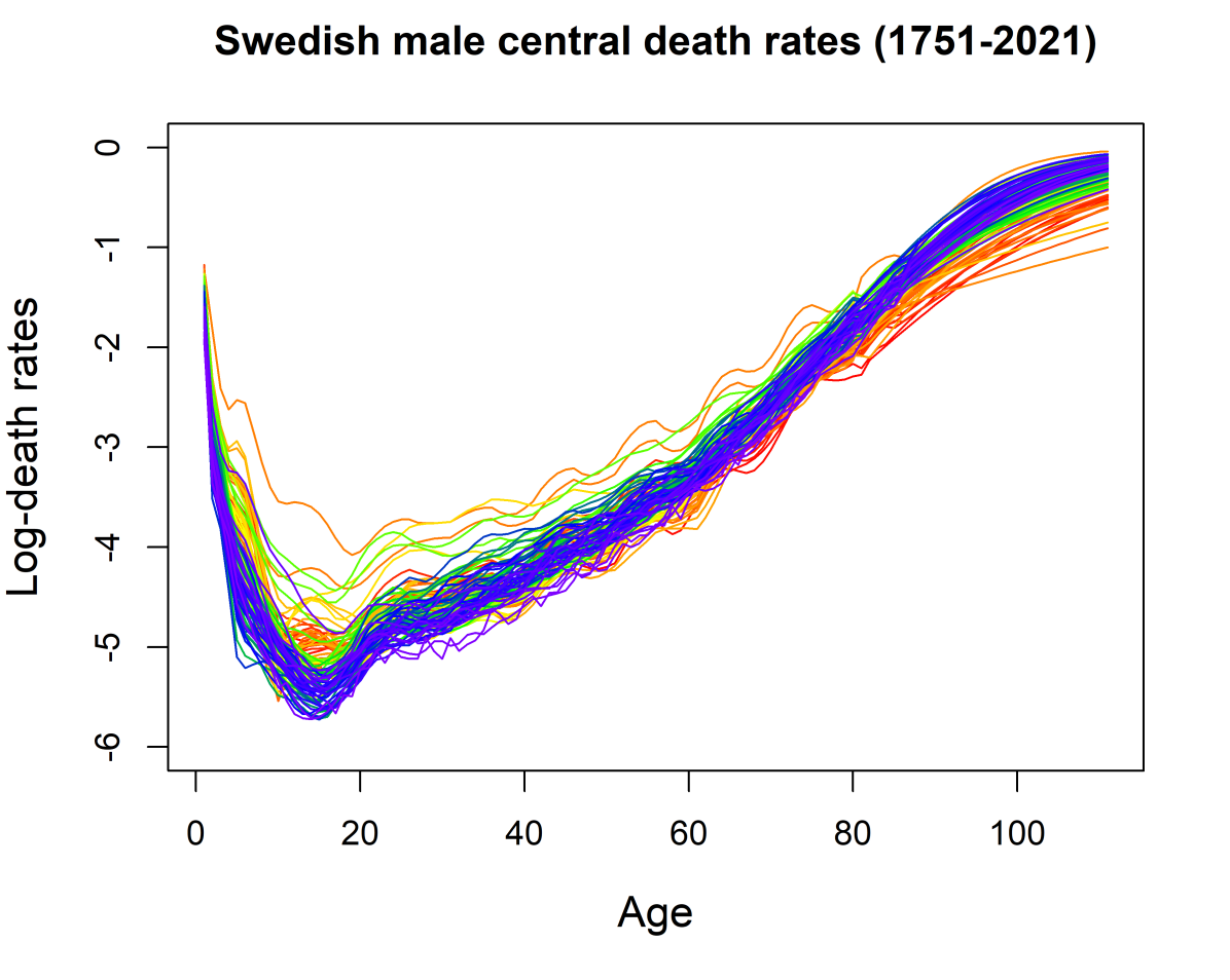
(a) Male data

(b) Female data

Figure 1: Log-mortality rates at various ages

Notes: The data for a specific year and gender is given by a 111-dimensional vector of mortality rates from age 0 to 110 (and older), and each of such vectors is plotted as a function of age.

For our statistical analysis, we first represent the observed mortality rates at various ages for each gender with 40 Legendre polynomial basis functions. We first estimate the memory parameter $d$ of the time series for each gender. The top rows of Table 6 report the local Whittle estimation results. As is not uncommon in many empirical applications, the memory of each time series is far greater than $1/2$ and quite closer to the unity. This not only implies that both time series of mortality rates are nonstationary but also justifies, to some degree, the conventional use of the random walk model for mortality in the literature. We then apply our variance-ratio testing procedure to estimate the dimension $q_{d}$ of the dominant subspace for each time series. Of course, to implement the proposed testing procedure, the asymptotic null distribution of the test statistic, which depends on $d$, needs to be approximated by a feasible estimate of $d$ (see Remark 4.4). This is done by replacing $d$ with the relevant estimate obtained by our proposed local Whittle method and reported in Table 6.

Table 6: Local Whittle estimation - Swedish mortality data.

Target	Method	Male	Female
$d$	Proposed	0.962	0.989
	LRS-type	0.956	0.978
$d-b$	Proposed	0.424	0.433
	LRS-type	0.402	0.275

Notes: The proposed and LRS-type estimators of $d$ are given as in Table LABEL:tab3, and the bandwidth $m$ is set to $\lfloor 1+T^{0.65}\rfloor$. The estimators of $d-b$ are given as in Table LABEL:tab4 with $m=\lfloor 1+T^{0.65}\rfloor$ but $\widehat{v}_{q_{d+1}}$ and $\widehat{v}_{q_{d+2}}$ are replaced by $\widehat{v}_{\widehat{q}_{d+1}}$ and $\widehat{v}_{\widehat{q}_{d+2}}$, where $\widehat{q}_{d+1}$ is the estimator obtained by our variance-ratio testing procedure.

Table 7: Dimension estimation - Swedish mortality data.

Target	Method	Male	Female
$q_{d}$	Proposed	5	5
	LRS-type	1	1
$q_{d-b}$	Proposed	6	4

Notes: The proposed estimator of $q_{d}$ is obtained by our variance-ratio testing procedure as in Table LABEL:tab1, and $K=q+2$, for each $H_{0}:q_{d}=q$, $\eta=0.05$, and $q_{\max}$ is set to $7$. The LRS-type estimator of $q_{d}$ is the same as that in Table LABEL:tab1, and the tuning parameter $K$ is set to $7$. The proposed estimator of $q_{d-b}$ is given as in Table LABEL:tab2, and $h$ is set to $\lfloor 1+T^{0.3}\rfloor$.