Heterotic de Sitter Beyond Modular Symmetry

Abstract

We study the vacua of $4d$ heterotic toroidal orbifolds using effective theories consisting of an overall Kähler modulus, the dilaton, and non-perturbative corrections to both the superpotential and Kähler potential that respect modular invariance. We prove three de Sitter no-go theorems for several classes of vacua and thereby substantiate and extend previous conjectures. Additionally, we provide evidence that extrema of the scalar potential can occur inside the PSL$(2,\mathbb{Z})$ fundamental domain of the Kähler modulus, in contradiction of a separate conjecture. We also illustrate a loophole in the no-go theorems and determine criteria that allow for metastable de Sitter vacua. Finally, we identify inherently stringy non-perturbative effects in the dilaton sector that could exploit this loophole and potentially realize de Sitter vacua.

1 Introduction

The accelerating expansion of the Universe SupernovaCosmologyProject:1998vns ; SupernovaSearchTeam:1998fmf and the nature of the dark energy driving it remain some of the greatest challenges in theoretical physics. The simplest mathematical model consistent with observations is that our universe is in a de Sitter (dS) phase and dark energy corresponds to a cosmological constant in Einstein’s equations. However, the scale of this constant is orders of magnitudes below naive expectations from the Standard Model of particle physics.

One might hope that natural explanations for the origin and scale of dark energy can be found in an ultraviolet complete theory of particle interactions and gravity. Our only viable candidate for such a theory is string theory, and so the quest for understanding the cosmological constant transmutes into a question of which string compactifications can yield four-dimensional dS cosmologies.

The construction of such cosmologies within string theory has been and remains one of the paramount tasks for string theory to connect to the low-energy physics of our universe. Existing construction schemes with still limited, but increasingly improved, control involve perturbative moduli stabilization with fluxes, branes and orientifold planes in dS vacua on negatively curved internal manifolds (such as twisted tori, product Riemann surfaces, and more general compact $6d$ hyperbolic spaces) as well as dS vacua on Calabi-Yau (CY) manifolds with fluxes and either purely non-perturbative or a mix of perturbative and non-perturbative quantum corrections stabilizing the volume moduli of the CY. For recent reviews providing a comprehensive overview as well as references to the original literature, see Silverstein:2016ggb ; Cicoli:2018kdo ; Flauger:2022hie .

While the viability of the various constructions is not completely settled, one could wonder if there exists some reason that dS vacua cannot exist at all in string theory Danielsson:2018ztv . Indeed, the refined dS conjecture Garg:2018reu ; Ooguri:2018wrx ; Hebecker:2018vxz as part of the Swampland program Vafa:2005ui posits that long periods of accelerated cosmological expansion are severely limited in quantum gravity and metastable dS minima are forbidden in asymptotic regions of the moduli space (the earlier, stronger dS conjecture Obied:2018sgi required modification due to explicit counter-examples Denef:2018etk ; Conlon:2018eyr ; Murayama:2018lie ; Choi:2018rze ; Hamaguchi:2018vtv ). The asymptotic dS conjecture can be thought of as a generalization of the Dine-Seiberg problem Dine:1985he in all directions of the moduli space. There is also an even weaker version of the dS conjecture, the Transplanckian Censorship Conjecture Bedroya:2019snp , which allows for short-lived dS minima residing in the interior of moduli space.

The above statements are conjectural, but they are motivated by a number of no-go results in the literature that forbid dS vacua in specific contexts. The classical $10d$ supergravity Maldacena-Nuñez no-go result Maldacena:2000mw suggests that any dS constructions must include non-classical ingredients as D-branes, O-planes, or quantum corrections. In the context of heterotic string theories, this no-go has been pushed farther to include stringy effects. The analysis in Covi:2008ea provides the general criterion which the Kähler manifolds of the volume moduli space of CY compactifications producing $4d$, ${\cal N}=1$ supergravity effective actions must fulfill to allow for metastable dS vacua to exist. This is a generalization of the Kähler geometry arguments provided in Gomez-Reino:2006tjy based on Brustein:2004xn .

Next, Green:2011cn considered the sub-leading $\alpha^{\prime}$ corrections arising from the modified Bianchi identity of the Neveu-Schwarz (NS) 2-form $B_{2}$ and concluded that dS vacua are not possible. This was further extended to an infinite tower of $\alpha^{\prime}$ contributions, where a perturbative calculation showed that AdS and dS are both ruled out Gautason:2012tb . Finally, the powerful worldsheet argument of Kutasov:2015eba ruled out any worldsheet effect giving rise to dS vacua at tree level in string perturbation theory.

Apart from worldsheet effects, string compactifications will have non-perturbative contributions in the string coupling $g_{s}$. Focusing again on heterotic constructions, a simple example is gaugino condensation, which has a generic strength of order $\delta\mathcal{L}\sim e^{-1/g_{s}^{2}}$. In Quigley:2015jia , partial no-go results were obtained ruling out AdS and dS solutions. However, this was not a comprehensive argument since threshold corrections Kaplunovsky:1987rp ; Dixon:1990pc ; Antoniadis:1991fh ; Antoniadis:1992rq ; Antoniadis:1992sa ; Kaplunovsky:1995jw and worldsheet instantons were not included, hence some heterotic constructions evade the no-go results Cicoli:2013rwa . There are some results incorporating gaugino condensation, threshold corrections, and worldsheet instantons in the context of toroidal orbifold compactifications of the heterotic string Gonzalo:2018guu ; Parameswaran:2010ec . The authors of Gonzalo:2018guu consider only the dilaton and overall Kähler modulus of the compactification. Using target space modular symmetry to enumerate all possible non-perturbative contributions, the authors find that AdS minima are generically present, while they argue numerically that no dS solutions can be realized. Note that Brustein:2004xn already contained in its Section II a limited version of the statements in Gonzalo:2018guu . On the other hand,  Parameswaran:2010ec considered all bulk moduli for certain orbifolds and numerically found only unstable dS extrema that satisfied the refined dS conjecture Olguin-Trejo:2018zun .

However, gaugino condensation is not the only non-perturbative contribution in $g_{s}$ present in the heterotic string theory. As argued by Shenker Shenker:1990 , all closed string theories generically have effects of strength $\delta\mathcal{L}\sim e^{-1/g_{s}}$. These are inherently stringy effects, in contrast to the purely quantum field theoretical nature of gaugino condensation. As the above arguments apply only to $\mathcal{O}(e^{-1/g_{s}^{2}})$ effects, examining these “Shenker-like” contributions to heterotic string vacua is the logical extension of previous no-go results.

In this work, we set our sights on this task. We will consider two-modulus models of heterotic toroidal orbifold compactifications and include Shenker-like effects as non-perturbative corrections to the dilaton Kähler potential $k(S,\bar{S})$. We will prove three no-go theorems that forbid dS vacua for different branches of solutions, and affirm several conjectures in Gonzalo:2018guu as corollaries. However, we find that on a separate branch of solutions, the Shenker-like effects may provide a loophole to the no-go theorems and permit heterotic dS vacua.

The paper is organized as follows. In Section 2, we review the relevant details of standard heterotic toroidal orbifold compactifications with a focus on the effective two-modulus model and the interplay of T-duality, threshold corrections, and non-perturbative effects. Then, we prove a no-go theorem that forbids de Sitter vacua for a class of extrema, even with Shenker-like effects included in the dilaton Kähler potential. In Section 3, we describe sufficient criteria to evade this no-go result and describe in detail the behavior of extrema in the fundamental domain of the Kähler modulus. In Section 4, we prove an additional no-go theorem and further restrict the classes of models that could contain dS vacua. We then review the scant literature on Shenker-like effects and show that they in principle satisfy the criteria to evade the no-go results we establish. We provide preliminary examples where dS vacua can be constructed in a bottom-up fashion. We also comment on a puzzle posed in Silverstein:1996xp on non-perturbative effects that are even stronger than those of Shenker at weak coupling. In Section 5, we conclude and discuss multiple future directions. In the appendices, we include supplemental information for the main text as well as proving a third no-go theorem in Appendix C for orbifolds with moduli mixing in the Kähler potential arising from anomaly cancellation.

2 Heterotic Orbifolds & A No-Go Theorem

In this section, we give a brief review of heterotic toroidal orbifolds, defining the set of four-dimensional effective theories considered throughout the paper. These consist of an overall Kähler modulus $T$ and dilaton $S$. Non-perturbative effects such as gaugino condensation and worldsheet instantons are captured by the superpotential $W(S,T)$ while the non-perturbative Shenker-like effects are captured by the dilaton Kähler potential $k(S,\bar{S})$. We then study the extrema of the scalar potential and prove a dS no-go theorem for a particular branch of extrema.

2.1 Simplified Heterotic Orbifold Models

We consider $\mathcal{N}=1$ supersymmetric toroidal orbifold models of the heterotic string, i.e. the heterotic string on $T^{6}/G$, where $G$ is the orbifold action defined by some discrete group. For $(2,2)$ constructions arising from standard embedding, the spectrum of these models includes the dilaton, $h^{1,1}$ Kähler moduli, $h^{2,1}$ complex structure moduli, gauge fields, and twisted and untwisted matter fields. General $(0,2)$ orbifolds contain the same untwisted moduli as the $(2,2)$ compactifications but with model-dependent twisted sector moduli.

Figure 1: The strict fundamental domain $\widetilde{\mathcal{F}}_{i}$ of the diagonal Kähler modulus $T_{i}$. The dots indicate the fixed points as well as the oft-quoted stabilized value $T_{i}\simeq 1.23i$ found in heterotic moduli stabilization.

Of critical importance is that the effective field theories (EFTs) of these orbifolds respect a target-space modular symmetry arising from T-duality Ferrara:1989bc ; Font:1990nt ; Cvetic:1991qm . If we consider for the moment the $T^{6}$ to be a factorized product of three $T^{2}$, then each of the diagonal Kähler moduli $T_{i}$ has a $\text{PSL}(2,\mathbb{Z})_{i}$ modular symmetry that acts as

$$T_{i}\rightarrow\gamma_{i}\cdot T_{i}=\frac{a_{i}T_{i}+b_{i}}{c_{i}T_{i}+d_{i}}\quad\text{ with }\quad\gamma_{i}=\begin{pmatrix}a_{i}&b_{i}\\ c_{i}&d_{i}\end{pmatrix}\in\text{PSL}(2,\mathbb{Z})_{i}\,.$$ (2.1)

Ostensibly, the Kähler moduli are valued in the upper half planes

$$\mathcal{H}_{i}=\{T_{i}\in\mathbb{C}\;\;|\;\;\text{Im}(T_{i})>0\}$$ (2.2)

since their vacuum expectation values (vevs) control the size of the compact dimensions. However, modular symmetry restricts the set of inequivalent $T_{i}$ values to the strict fundamental domain $\widetilde{\mathcal{F}}_{i}$, which is defined as the union of the set

$$\mathcal{F}_{i}=\bigg{\{}T_{i}\in\mathcal{H}_{i}\;\;\rvert\;\;\lvert T_{i}\rvert>1\;\;\&\;\;\lvert\text{Re}(T_{i})\rvert<\frac{1}{2}\bigg{\}}\,,\quad$$ (2.3)

with boundary points that satisfy $\text{Re}(T_{i})<0$. This is the region displayed in Fig. 1. Of particular note are the fixed points $T_{i}=i$ and $T_{i}=e^{2\pi i/3}\equiv\rho$, which are fixed by cyclic subgroups of $\text{PSL}(2,\mathbb{Z})_{i}$, as described in Appendix A.

The matter fields $\Phi_{\alpha}$ of the compactification also transform under modular transformations as

$$\Phi_{\alpha}\rightarrow e^{\sum_{i}n_{\alpha}^{i}\mathcal{J}_{i}(T_{i})}\Phi_{\alpha}\,,\quad$$ (2.4)

where $\mathcal{J}_{i}(T)=\ln(c_{i}T_{i}+d_{i})$ and the numbers $n_{\alpha}^{i}$ are the weights of the matter field. For an arbitrary orbifold, the modular symmetry group may not be a simple product of $\text{PSL}(2,\mathbb{Z})$ factors. For example, if one introduces discrete Wilson lines or orbifolds where the $6d$ lattice is not a simple direct sum, then the duality group will in general be a congruence subgroup of $\text{PSL}(2,\mathbb{Z})$ Love:1996sk ; Mayr:1993mq . Irrespective of the precise form of the modular symmetry group, the effective action and the scalar potential

$$V=e^{\mathcal{K}}\left(\mathcal{K}^{a\bar{b}}F_{a}\bar{F}_{\bar{b}}-3W\bar{W}\right)$$ (2.5)

must be modular functions, i.e. they should transform as modular forms of weight $(0,0)$: $V(\gamma\cdot T_{i},\gamma\cdot\bar{T}_{i},...)=V(T_{i},\bar{T}_{i},..)$. Here $\mathcal{K}$ and $W$ are the Kähler potential and superpotential, respectively, and the $F_{a}$ are the F-terms of the fields, defined below. The above condition can also be cast as the restriction that the defining supergravity function $\mathcal{G}=\mathcal{K}+\ln\lvert W\rvert^{2}$ is modular invariant.

In the following, we shall neglect all of the moduli and matter fields except for an overall diagonal Kähler modulus, $T$, and the dilaton. We shall also neglect Wilson lines and therefore take the modular symmetry of the effective field theory to be $\text{PSL}(2,\mathbb{Z})$. The Kähler potential of this two-modulus EFT is

$$\mathcal{K}=k(S,\bar{S},T,\bar{T})-3\ln\left(-i(T-\bar{T})\right)\,.$$ (2.6)

For the moment, we are using the familiar chiral multiplet formalism for the dilaton with $S$ being its chiral superfield representation consisting of a scalar (the dilaton), a pseudoscalar (from dualizing the NS 2-form $B_{2}$), a Weyl spinor, and an auxiliary field. The function $k(S,\bar{S},T,\bar{T})$ is the Kähler potential for the dilaton, which may have dependence on $T$, as discussed below. At tree-level, there is no $T$-dependence in the dilaton Kähler potential, hence $k(S,\bar{S},T,\bar{T})=-\ln(S+\bar{S})$ and the $4d$ universal gauge coupling is

$$\frac{g_{4}^{2}}{2}=\bigg{\langle}\frac{1}{S+\bar{S}}\bigg{\rangle}\,.$$ (2.7)

Under modular transformations, the combination $T-\bar{T}$ transforms as a weight $(-1,-1)$ modular form since $(T-\bar{T})\rightarrow\lvert cT+d\rvert^{-2}(T-\bar{T})$. Then assuming that $k(S,\bar{S},T,\bar{T})$ is inert under $\text{PSL}(2,\mathbb{Z})$, the Kähler potential undergoes a Kähler transformation

$$\mathcal{K}\rightarrow\mathcal{K}+3\mathcal{J}(T)+3\bar{\mathcal{J}}(\bar{T}),$$ (2.8)

where $\mathcal{J}(T)$ is the same as in the phase of Eq. 2.4 but with the indices removed. The invariance condition on $\mathcal{G}$ then implies that the superpotential must transform as a weight $(-3,0)$ modular form Ferrara:1989bc :

$$W(S,\gamma\cdot T)=e^{i\delta(\gamma)}(cT+d)^{-3}W(S,T)\,.$$ (2.9)

Technically, we allow the superpotential to furnish a projective representation of $\text{PSL}(2,\mathbb{Z})$ and so it may transform as a weight $(-3,0)$ modular form up to the phase $\delta(\gamma)$, which depends only on the matrix $\gamma\in\text{PSL}(2,\mathbb{Z})$.

As we are neglecting matter fields, the superpotential we are considering is non-perturbative in nature and arises from gaugino condensation of some subgroups of the $10d$ heterotic gauge sector. If the gauge group factor $G_{a}$ undergoes gaugino condensation, a non-perturbative superpotential is generated of the form

$$W\sim e^{-f_{a}/b_{a}}\,.$$ (2.10)

Here $f_{a}$ is the gauge kinetic function for $G_{a}$ and the coefficient $b_{a}$ is related to the beta function of $G_{a}$ as $\mu\frac{dg_{a}}{d\mu}=-\frac{3}{2}b_{a}g_{a}^{3}$ and is given by

$$b_{a}=\frac{1}{8\pi^{2}}\left(C_{a}-\frac{1}{3}\sum_{\alpha}C^{\alpha}_{a}\right)\,,\quad$$ (2.11)

where $C_{a}$ and $C^{\alpha}_{a}$ are the quadratic Casimirs of the adjoint and the $\alpha$-th matter sectors, respectively. At tree level, $f_{a}=k_{a}S$, with $k_{a}$ the level of the Kac-Moody algebra underlying the gauge group $G_{a}$. In this form, it is not clear that Eq. 2.10 transforms with weight $(-3,0)$ since naively the dilaton is invariant under modular transformations.

This situation is remedied by taking into account the 1-loop effects of threshold corrections Kaplunovsky:1987rp ; Dixon:1990pc ; Antoniadis:1991fh ; Antoniadis:1992rq ; Antoniadis:1992sa ; Kaplunovsky:1995jw and anomaly cancellation Derendinger:1991hq ; Lust:1991yi ; LopesCardoso:1991wk ; LopesCardoso:1991ifk ; LopesCardoso:1992yd ; deCarlos:1992kox . The physical origins of these effects are quite simple – the fermions in the $4d$ theory undergo modular transformations and generally lead to non-zero anomalies that must be canceled by the $4d$ Green-Schwarz mechanism. Furthermore, if the orbifold has $\mathcal{N}=2$ subsectors, integrating out the heavy string states will lead to moduli-dependent corrections to the gauge kinetic function. To incorporate these contributions to the effective model, we include a correction into the gauge kinetic function

$$f_{a}=k_{a}S+\left(b^{\prime}_{a}-\frac{1}{3}k_{a}\delta_{GS}\right)\ln\eta^{6}(T)+\cdots\,,\quad$$ (2.12)

and to the dilaton Kähler potential

$$-\ln(S+\bar{S})\rightarrow-\ln\bigg{(}S+\bar{S}+\delta_{GS}\ln\left(-i(T-\bar{T})\right)\bigg{)}\,.$$ (2.13)

The coefficient $b_{a}^{\prime}$ is determined by the quadratic Casimirs and the modular weights of the matter fields charged under $G_{a}$:

$$b_{a}^{\prime}=\frac{1}{8\pi^{2}}\left(C(G^{a})-\sum_{\alpha}C^{\alpha}_{a}(1+2n_{\alpha})\right)\,.$$ (2.14)

The dilaton now transforms as

$$S\rightarrow S+\delta_{GS}\ln(cT+d)$$ (2.15)

under $\text{PSL}(2,\mathbb{Z})$ in order to maintain modular invariance of the action. If we neglect matter fields, as in the case of a hidden $E_{8}$ condensate, then inserting Eq. 2.12 into Eq. 2.10 yields

$$W\sim\frac{e^{-k_{a}S/b_{a}}}{\left(\eta(T)\right)^{6-\frac{2k_{a}\delta_{GS}}{b_{a}}}}\,.$$ (2.16)

As described in Appendix A, $\eta(T)$ transforms with weight $(1/2,0)$, and combining this fact with Eq. 2.15 we see that the superpotential transforms with weight $(-3,0)$ and the scalar potential will be invariant under modular transformations. Hence, threshold corrections and anomaly cancellation are essential ingredients in the consistency of the $4d$ EFT arising from the heterotic string.

While the above makes the consistency of modular invariance in the EFT clear, it will be convenient for our purposes to adopt a convention where the dilaton is inert under modular transformations. One is free to re-define the dilaton via a holomorphic function of other moduli Kaplunovsky:1995jw ; Derendinger:1991hq – in particular, we can re-define the dilaton via

$$S\rightarrow S+\delta_{GS}\ln\eta^{2}(T)\,.$$ (2.17)

This eliminates the dependence of the superpotential on $\delta_{GS}$ so that all information on anomaly cancellation in encoded in the re-defined Kähler potential.

However, the superpotential obtained from Eq. 2.16 with Eq. 2.17 is still too primitive – as the dots in Eq. 2.12 suggest, there are additional contributions to the threshold corrections Kaplunovsky:1995tm ; Kiritsis:1996dn . These are moduli-dependent but transform trivially under $\text{PSL}(2,\mathbb{Z})$. One can push the power of modular invariance even further to parametrize these effects. After the dilaton re-definition in Eq. 2.17, the Dedekind etas saturate the transformation law of the superpotential, but the numerator could involve a function of $T$ that is modular invariant (up to a phase). Then a general non-perturbative superpotential satisfying the T-duality requirement has the form

$$W(S,T)=\frac{\Omega(S)H(T)}{\eta^{6}(T)}\,.$$ (2.18)

Here $H(T)$ is a modular function with a potentially non-trivial multiplier system. If $H(T)$ is regular in the fundamental domain, a theorem 10.2307/1968796 ; Lehner:1964 states that it has the parametrization

$$H(T)=\bigg{(}\frac{G_{4}(T)}{\eta^{8}(T)}\bigg{)}^{n}\bigg{(}\frac{G_{6}(T)}{\eta^{12}(T)}\bigg{)}^{m}\mathcal{P}(j(T))\,,\quad$$ (2.19)

with $G_{4}(T)$ and $G_{6}(T)$ the weight $(4,0)$ and $(6,0)$ holomorphic Eisenstein series and $j(T)$ the $j$-invariant (see Appendix A). $\mathcal{P}(x)$ is a polynomial, and without loss of generality we take $\mathcal{P}(0)\neq 0$ and $\mathcal{P}(1728)\neq 0$. In Eq. 2.18, we can technically allow an arbitrary function for $\Omega(S)$, but we will mostly consider it as arising from gaugino condensation and one should think of it as having the generic form $\Omega(S)=h+e^{-S/b_{a}}$ for a single condensate, with $h$ an additive constant to describe $H_{3}$-flux, or $\Omega(S)=\sum_{a}e^{-S/b_{a}}$ for a racetrack scenario. This superpotential was first proposed in Cvetic:1991qm .

Note that the terms in $H(T)$ have the schematic form of $\delta\mathcal{L}\sim e^{\pm 2\pi iT}$ – the function $H(T)$ can be thought of parametrizing non-perturbative effects in the Kähler modulus. Thus the superpotential in Eq. 2.18 parametrizes non-perturbative effects in the superpotential for both moduli in the effective model.

The above discussion defines a broad class of effective heterotic toroidal orbifold models via the superpotential in Eq. 2.18 and the Kähler potential from Eq. 2.6 with

$$k(S,\bar{S},T,\bar{T})\supset-\ln\bigg{(}S+\bar{S}+\delta_{GS}\ln\left(-i(T-\bar{T})\lvert\eta(T)\rvert^{4}\right)\bigg{)}\,.$$ (2.21)

It is instructive to consider two extreme cases. For the simple $\mathbb{Z}_{3}$ orbifold with an $E_{8}$ condensate, there is no $\mathcal{N}=2$ subsector and $\delta_{GS}=3b_{E_{8}}/k_{E_{8}}$. If we consider the formalism where the dilaton transforms under $\text{PSL}(2,\mathbb{Z})$, we see that the exponent of the Dedekind eta in Eq. 2.16 vanishes and the modular transformation properties of the superpotential are encoded entirely in the dilaton. In the formalism where the dilaton is invariant, the superpotential has factors of Dedekind eta, but these vanish at the level of the scalar potential when the original dilaton variable is used. These features are reflections of the usual statement that the $\mathbb{Z}_{3}$ (and $\mathbb{Z}_{7}$) orbifolds lack $\mathcal{N}=2$ subsectors and therefore have no moduli-dependent threshold corrections Dixon:1990pc . On the opposite end of the spectrum, the $\mathbb{Z}_{2}\times\mathbb{Z}_{2}$ orbifold with standard embedding has $\delta_{GS}=0$, so the dilaton is invariant under $\text{PSL}(2,\mathbb{Z})$ without any redefinition and the Dedekind etas are required in the superpotential and scalar potential. These two examples illustrate the diverse ways in which heterotic orbifolds conspire to maintain modular symmetry in spite of effects that naively break the duality.

We now largely restrict ourselves to a particular subclass of the models described above. In particular, we will neglect the $T$-dependent correction to the dilaton Kähler potential arising from anomaly cancellation and set the dilaton-dependent term in Eq. 2.6 to

$$k(S,\bar{S},T,\bar{T})=k(S,\bar{S})=-\ln(S+\bar{S})+\delta k(S,\bar{S})\,.$$ (2.22)

By the inclusion of the additional term $\delta k(S,\bar{S})$, we have in mind incorporating non-perturbative contributions arising from Shenker-like effects, as mentioned in the Introduction and further described in Section 4. For the superpotential we take the general form in Eq. 2.18. We consider $T$-dependent Kähler potential corrections in Section 4, and we return to the general case of Eq. 2.21 in Appendix C.

Using Eqs. 2.6, 2.22 and 2.18, the F-term supergravity scalar potential is

$$\begin{split}V(T,S)&=e^{\mathcal{K}}\left(\mathcal{K}^{S\bar{S}}F_{S}\bar{F}_{\bar{S}}\,+\,\mathcal{K}^{T\bar{T}}F_{T}\bar{F}_{\bar{T}}\,-\,3W\bar{W}\right)\\ &=e^{k(S,\bar{S})}\,Z(T,\bar{T})\,\lvert\Omega(S)\rvert^{2}\,\left[\left(A(S,\bar{S})-3\right)\lvert H(T)\rvert^{2}+\widehat{V}(T,\bar{T})\right]\,,\quad\end{split}$$ (2.23)

where we defined

$$A(S,\bar{S}) =\frac{k^{S\bar{S}}F_{S}\bar{F}_{\bar{S}}}{\lvert W\rvert^{2}}=\frac{k^{S\bar{S}}\lvert\Omega_{S}+K_{S}\Omega\rvert^{2}}{\lvert\Omega\rvert^{2}}\,,\quad$$ (2.24)

$$\widehat{V}(T,\bar{T}) =\frac{-(T-\bar{T})^{2}}{3}\,\bigg{\lvert}H_{T}(T)-\frac{3i}{2\pi}H(T)\widehat{G}_{2}(T,\bar{T})\bigg{\rvert}^{2}\,,\quad$$ (2.25)

$$Z(T,\bar{T}) =\frac{1}{i(T-\bar{T})^{3}\lvert\eta(T)\rvert^{12}}\,,\quad$$ (2.26)

with subscripts denoting derivatives and $k^{S\bar{S}}=(k_{S\bar{S}})^{-1}$. We have also introduced the non-holomorphic Eisenstein series of weight $(2,0)$, $\widehat{G}_{2}(T,\bar{T})$ (see Appendix A). Note that each of the functions defined in Eqs. 2.24, 2.25 and 2.26 are modular invariant.

This potential has been discussed in several contexts in the literature. Originally in Font:1990nt ; Cvetic:1991qm as an effective field theory for heterotic phenomenology, then in the context of relating swampland conjectures to modular symmetry in Gonzalo:2018guu , and recently in a study to connect flavor symmetry and modular symmetry Novichkov:2022wvg . A fascinating feature of this potential is that it diverges in the limit $\text{Im}(T)\rightarrow\infty$. This has interesting implications for the Swampland Distance Conjecture Ooguri:2006in , as observed in Gonzalo:2018guu ; Cribiori:2022sxf . In the following, our discussion will align mostly with the first two contexts – we will study vacua of the above potential with Shenker-like terms included via $k(S,\bar{S})$.

2.2 Extrema of the Two-Modulus Model

In this section, we study the vacua of the two-modulus heterotic model with the potential in Eq. 2.23. Several aspects of the vacua have been studied in great detail in Font:1990nt ; Cvetic:1991qm ; Gonzalo:2018guu . We now review relevant details of those discussions.

An important feature of the scalar potential in Eq. 2.23 is that it is a modular function – that is, the scalar potential is invariant under the $\text{PSL}(2,\mathbb{Z})$ transformation defined in Eq. 2.1. In addition to restricting the form of the non-perturbative superpotential, the power of modular symmetry also guides the search for vacua. Since $dT$ transforms as $dT\rightarrow(cT+d)^{-2}dT$ under modular transformations, $\partial V/\partial T$ is a weight $(2,0)$ non-holomorphic modular form. As shown in Appendix A, weight $(2,0)$ modular forms vanish at the $\text{PSL}(2,\mathbb{Z})$ fixed points $T=i$ and $T=e^{2\pi i/3}\equiv\rho$. Thus

$$\partial_{T}V(S,T)\rvert_{T=i,\rho}=0\,,\quad$$ (2.27)

and the fixed points are always extrema in the $T$-sector. Modular symmetry also simplifies the analysis of the critical points at the fixed points – the mixed derivatives of $S$ and $T$ are also weight $(2,0)$ modular forms, and so

$$\partial_{S}\partial_{T}V(S,T)\rvert_{T=i,\rho}=\partial_{\bar{S}}\partial_{T}V(S,T)\rvert_{T=i,\rho}=0\,.$$ (2.28)

The Kähler modulus sector can also have critical points away from the fixed points, but such points are more difficult to analyze since modular symmetry does not assist and their treatment must be purely numerical. Thus we can partially categorize extrema by the value of their Kähler modulus vev as follows:

$$\text{Class 1: }\,\quad\hskip 0.28436pt\langle T\rangle=i\,,\quad$$ (2.29)

$$\text{Class 2: }\,\quad\langle T\rangle=\rho\,,\quad$$ (2.30)

$$\text{Class 3: }\,\quad\langle T\rangle\neq i,\rho\,.$$ (2.31)

It was conjectured Cvetic:1991qm that all critical points lie on either the boundary of the fundamental domain of $T$ or the line $\text{Re}(T)=0$. However, Novichkov:2022wvg disputes this conjecture by finding minima inside the fundamental domain and close to the fixed point $\rho$. We reinforce these results by finding multiple saddle points inside the fundamental domain, as discussed in Section 3.3.

To completely understand the vacua, we must also consider the dilaton sector. Our goal will be to examine dS vacua, which can only be achieved if one or both of the F-terms

$$F_{S} =\frac{H(T)}{\eta^{6}(T)}(\Omega_{S}+k_{S}\Omega)\equiv\frac{H(T)}{\eta^{6}(T)}\widetilde{F}_{S}\,,\quad$$ (2.32)

$$F_{T} =\frac{\Omega(S)}{\eta^{6}(T)}\bigg{(}H_{T}-\frac{3i}{2\pi}\widehat{G}_{2}H\bigg{)}\equiv\frac{\Omega(S)}{\eta^{6}(T)}\widetilde{F}_{T}\,,\quad$$ (2.33)

are non-zero. We have also introduced the re-scaled F-terms $\widetilde{F}_{S}$ and $\widetilde{F}_{T}$ for later convenience. We can then further categorize vacua according to whether or not they force the dilaton F-term to vanish:

$$\text{Class A: }\,\quad\widetilde{F}_{S}=\Omega_{S}+k_{S}\Omega=0\,,\quad$$ (2.34)

$$\text{Class B: }\,\quad\widetilde{F}_{S}\neq 0,$$

$$\hskip 59.75095pt\Omega_{SS}=\bar{\Omega}e^{2i\sigma}k_{S\bar{S}}\left(2-\frac{1}{\lvert H\rvert^{2}}\widehat{V}(T,\bar{T})\right)+\left(\frac{k_{SS\bar{S}}}{k_{S\bar{S}}}-k_{S}\right)\widetilde{F}_{S}-k_{SS}\Omega-k_{S}\Omega_{S}\,.$$ (2.35)

Here we have defined $\sigma=\text{arg}(\Omega_{S}+k_{S}\Omega)$. Note that both of the above conditions solve $\partial_{S}V(S,T)=0$, and it is assumed that $H(T)$ is non-vanishing for Class B extrema.

The Class A extrema simply correspond to the vanishing of the dilaton F-term. Thus to have any hope of achieving a vacuum with positive energy, along this branch we demand $F_{T}\neq 0$. If we again consider the simple case of a single gaugino condensate, such an extremum would require a non-physical negative string coupling constant. This is the motivation behind racetrack models, where the Class A solution corresponds to stabilization of the dilaton by balancing two gaugino condensates against one another. With $H(T)=1$, a vacuum exists for Class A solutions at the point $T\simeq 1.23i$, which is the typical stabilized value found in heterotic models. Note that for Class A solutions, the Hessian is block diagonal, independent of the value of $T$. This point is discussed in more detail in the next subsection and is a crucial aspect of the no-go theorem we prove there.

For Class B solutions, we can allow $F_{T}$ to vanish since positive energy could be achieved by the dilaton sector. These solutions are somewhat more unfamiliar as they do not follow this simple picture arising from racetracks and one must introduce a means to stabilize the dilaton and generate a non-zero F-term. This can be achieved by the Shenker-like terms in $k(S,\bar{S})$. The study of these extrema is the subject of Section 3 and mechanisms to generate these vacua are discussed in Section 4.

Using the above categories, we organize potential dS extrema of the two-modulus theory into 6 classes: Class A-1, A-2, and A-3 extrema, which are SUSY-preserving in the dilaton direction, and Class B-1, B-2, and B-3 extrema, which instead break SUSY in the dilaton sector. Further refinements of each class are possible since the type of critical point in general depends on the integers $m$ and $n$ and the polynomial $\mathcal{P}(j(T))$ in Eq. 2.19.

The Class A-1, A-2, and A-3 extrema were examined in Cvetic:1991qm ; Gonzalo:2018guu . If one assumes that the dilaton is stabilized, then the analysis of these extrema reduces to examination of the Kähler modulus sector. The authors of Cvetic:1991qm ; Gonzalo:2018guu prove that the fixed points are never dS minima – that is, there are no dS minima in Class A-1 and A-2 extrema. As for Class A-3, Gonzalo:2018guu argues that numerically they do not find dS minima and conjecture that they do not exist. We now verify this conjecture by proving a no-go theorem.

2.3 Class A de Sitter No-Go Theorem

We now prove a no-go theorem that illustrates the impossibility of obtaining dS vacua via Class A solutions of the two-modulus model above. As a corollary, we will verify and extend the results of Gonzalo:2018guu .

Theorem 1.

At a point $(T_{0},S_{0})$, the scalar potential $V(T,S)$ in Eq. 2.23
                can not simultaneously satisfy:

1. $V(T_{0},S_{0})>0$

2. $\partial_{S}V(T_{0},S_{0})=0\quad\&\quad\partial_{T}V(T_{0},S_{0})=0$

3. $(\Omega_{S}+k_{S}\Omega)\rvert_{S=S_{0}}=0$

4. Eigenvalues of the Hessian of $V(T,S)$ at $(T_{0},S_{0})$ are all $\geq 0$.

Proof.

The proof proceeds by contradiction – let us assume that (i)-(iv) are true at $(T_{0},S_{0})$. The first derivative of $V(T,S)$ with respect to $S$ is

$$\partial_{S}V(T,S)=\frac{F_{S}}{W}V(T,S)+\left\{e^{k(S,\bar{S})}\lvert\Omega(S)\rvert^{2}\lvert H(T)\rvert^{2}Z(T,\bar{T})\right\}\partial_{S}A(S,\bar{S})\,.$$ (2.36)

Since $F_{S}\propto\Omega_{S}+k_{S}\Omega$, (iii) manifestly implies the vanishing of the first term. The derivative $\partial_{S}A(S,\bar{S})$ contains several terms, but each term is proportional to either $F_{S}$ or its conjugate, and so the second term above also vanishes. Thus (iii) implies the vanishing of the above derivative at $(T_{0},S_{0})$. This is simply a verification that (iii) defines Class A extremum. To be consistent with (i), we require that $\widetilde{F}_{T}(T_{0})\neq 0$ and $\Omega(S_{0})\neq 0$. Then without loss of generality we can introduce a parameter $\Lambda>0$ and recast (i) as

$$V(T_{0},S_{0})=e^{k_{0}}\lvert\Omega_{0}\rvert^{2}Z_{0}\Lambda^{4}\,,\quad$$ (2.37)

where the subscript denotes evaluation at $(T,S)=(T_{0},S_{0})$. This can be interpreted as an equation for $H_{T}(T_{0})$ and is solved by

$$H_{T}(T_{0})=\frac{3i}{2\pi}H_{0}\widehat{G}_{2}(T_{0},\bar{T}_{0})\pm\frac{\sqrt{3}i}{T_{0}-\bar{T}_{0}}\bigg{(}\Lambda^{2}\!\pm i\sqrt{\lvert H_{0}\rvert^{2}\left(3-A(S_{0},\bar{S}_{0})\right)}\bigg{)}\,.$$ (2.38)

In this expression, any of the four sign combinations is valid, and we have taken $A(S_{0},\bar{S}_{0})<3$. This is not an assumption since technically (iii) implies that $A(S_{0},\bar{S}_{0})=0$, but we will carry it in our expressions for the moment and take the appropriate limit at the end. Similarly, the $\partial_{T}V(T_{0},S_{0})$ requirement of condition (ii) yields an algebraic equation for $H_{TT}(T_{0})$ that can be solved. We give this condition in Section B.1. Moving onto condition (iv), we first note that Eq. 2.36 and (iii) imply that

$$\partial_{T}^{k}\partial_{\bar{T}}^{l}\partial_{S}V(T_{0},S_{0})=0\quad\quad\forall\,\,k,\,l\in\mathbb{N}_{+}\,.$$ (2.39)

Thus the Hessian of $V(T,S)$ is block diagonal, with the blocks corresponding to the $T$ and $S$ sectors. Then the eigenvalues of the Hessian are simply the eigenvalues of the two blocks. We focus on the Kähler modulus block – in terms of the real and imaginary components of $T=a+it$, its components are

$$\partial^{2}_{t}V =2\partial_{T}\partial_{\bar{T}}V-2\text{Re}(\partial_{T}^{2}V)\,,\quad$$ (2.40)

$$\partial_{a}^{2}V =2\partial_{T}\partial_{\bar{T}}V+2\text{Re}(\partial_{T}^{2}V)\,,\quad$$ (2.41)

$$\partial_{t}\partial_{a}V =-2\text{Im}(\partial_{T}^{2}V)\,.$$ (2.42)

Computing the $T$ derivatives and plugging in the expressions derived above for $H_{T}(T_{0})$ and $H_{TT}(T_{0})$, we find

$$\partial_{T}\partial_{\bar{T}}V(T_{0},S_{0}) =\frac{2e^{k_{0}}\lvert\Omega_{0}\rvert^{2}Z_{0}}{(T_{0}-\bar{T}_{0})^{2}}\bigg{(}\Lambda^{4}(2-3A(S_{0},\bar{S}_{0}))-\lvert H_{0}\rvert^{2}A(S_{0},\bar{S}_{0})\bigg{)}$$ (2.43)

$$\longrightarrow\frac{-2e^{k_{0}}\lvert\Omega_{0}\rvert^{2}Z_{0}}{-(T_{0}-\bar{T}_{0})^{2}}\Lambda^{4}\,.$$ (2.44)

In going to the second line, we have enforced the vanishing of $A_{0}$ as demanded by (iii), the Class A extremum condition. We see that $\partial_{T}\partial_{\bar{T}}V(T_{0},S_{0})<0$ for all values of $T_{0}$ and functions $H(T)$. Thus, it must be that $\partial_{t}^{2}V(T_{0},S_{0})<0$ or $\partial_{a}^{2}V(T_{0},S_{0})<0$. In either case, the determinant of the Kähler modulus block of the Hessian is negative. This immediately implies that one of the eigenvalues of the Hessian is negative, in contradiction with (iv). We can also consider the case of a vanishing $T$-block determinant, which could occur if

$${\text{Re}\,}\!(\partial_{T}^{2}V(T_{0},S_{0}))=\pm\frac{2e^{k_{0}}\lvert\Omega_{0}\rvert^{2}Z_{0}}{(T_{0}-\bar{T}_{0})^{2}}\Lambda^{4}\;\;\quad\&\;\;\quad{\text{Im}\,}\!(\partial_{T}^{2}V(T_{0},S_{0}))=0\,.$$ (2.45)

However, the vanishing of the Kähler sector determinant for this case occurs only because one of its two eigenvalues vanishes. Even in this degenerate case, the other eigenvalue is necessarily nonzero and negative, again in contradiction with (iv). Thus (iv) is incompatible with (i)-(iii) and the theorem is demonstrated. Since conditions (i)-(iv) are the requirements for a Class A dS vacuum, the theorem demonstrates that such vacua are impossible. ∎

The above result deserves several comments. First, the above is a proof that dS vacua cannot occur anywhere in the fundamental domain of $T$ if $\widetilde{F}_{S}=0$. This is equivalent to the statement that no non-perturbative superpotential in the class defined by Eq. 2.18 and Eq. 2.19 can lift a racetrack vacuum to positive energy. This is true even if Shenker-like effects are present in the Kähler potential, assuming they enter only through $k(S,\bar{S})$. This is a limited extension of previous no-go results mentioned in the introduction to non-perturbative corrections of strength $\mathcal{O}(e^{-1/g_{s}})$. Second, we immediately have two straightforward corollaries:

Corollary 1.1.

Class A extrema in the two-modulus model with
                    $k(S,\bar{S})=-\ln(S+\bar{S})$ can never be dS vacua.

Corollary 1.2.

The one-modulus model with $W(T)=H(T)/\eta^{6}(T)$ and
                    $\mathcal{K}=-3\ln(-i(T-\bar{T}))$ can not have dS vacua.

The latter follows by taking the appropriate limits to remove the dilaton in the proof of Theorem 1. These corollaries verify the conjectures in Gonzalo:2018guu that state that neither Class A extrema nor the single-modulus model can have dS vacua.

We also observe that the above proof does not make use of the modular properties of $H(T)$ in any meaningful way. We posit that the lack of Class A dS vacua is more tied to the structure of Class A extrema and the factorized form of the superpotential and Kähler potential.

Next, we note that if we were to assume that $(T_{0},S_{0})$ was an AdS minimum by replacing $\Lambda^{4}\rightarrow-\Lambda^{4}$, then the no-go theorem does not apply because manifestly $\partial_{T}\partial_{\bar{T}}V(T_{0},S_{0})>0$ – the very argument that forbids dS minima cleanly allows for AdS minima.

Finally, the above no-go provides a hint as to how one might obtain dS vacua in these heterotic compactifications – one must consider Class B solutions where the dilaton F-term is non-vanishing. In the next section, we explore constraints on Class B extrema such that dS vacua exist in the two-modulus model.

3 Circumventing the No-Go

In this section, we study the branch of extrema that evade the no-go result of the previous section – namely, Class B extrema. We will assume that the dilaton is stabilized and determine under what conditions the Kähler modulus sector is stabilized with positive energy. This will translate into bounds on the function $A(S,\bar{S})$, which depends on the Shenker-like effects via $k(S,\bar{S})$. For Class B-1 and B-2 extrema, which occur at the fixed points, this analysis is valid due to the block diagonal structure of the Hessian required by modular invariance, as discussed in Section 2. At general points in the fundamental domain, corresponding to Class B-3 extrema, the Hessian is in general not block diagonal and one must treat the $T$ and $S$ moduli together. For these extrema, we will examine minima of the single-modulus model containing only $T$ and discuss the plausibility of uplifting them via the dilaton subsector. In doing so, we will present evidence disproving a previous conjecture on the nature of extrema in the fundamental domain of $T$. We will turn to the issue of stabilizing the dilaton sector in the following section.

Figure 2: Summary of dS vacua possibilities at the fixed points with respect to the integers $(m,n)$ in $H(T)$ assuming the dilaton is stabilized. At $(0,0)$, both fixed points can have a dS vacuum. For $(m,0)$, $T=\rho$ is a dS minimum if $A(S,\bar{S})>3$. For $(0,n)$, $T=i$ can be a dS vacuum for a window of $A(S,\bar{S})$ values that increases with $n$ and is dependent on $\mathcal{P}(j(T))$. The cases $(1,n)$ or $(m,1)$ result in unstable dS extrema. Finally, we always have Minkowski extrema at the self dual points when $(m,n)>(1,1)$.

3.1 Class B-1 Vacua: $T=i$

We start by examining extrema at the fixed point $T=i$. If the integer $m$ in Eq. 2.10 is greater than one, then both $H(T)$ and $\widehat{V}(T,\bar{T})$ vanish at $T=i$ and so the extremum is Minkowski. Therefore, in the remainder of this section we will study the potential for the cases $m=0$ and $m=1$.

m = 0 :

The potential evaluated at $T=i$ has the compact form

$$V(S,\bar{S},i,-i)=\frac{2^{4n+9}\pi^{8n+9}}{3^{2n}5^{2n}\Gamma^{12}(1/4)}\lvert\Omega(S)\rvert^{2}\lvert\mathcal{P}(1728)\rvert^{2}e^{k(S,\bar{S})}\left(A(S,\bar{S})-3\right)\,,\quad$$ (3.1)

and we see then that a dS extremum requires $A(S,\bar{S})>3$. To examine the stability of the extremum, we calculate the second order derivatives in the fields $t,\,a$ from $T=a+it$ as

$$\begin{split}\partial_{t/a}^{2}V\rvert_{T=i}=&\frac{4^{2n+4}\pi^{8n+9}e^{k(S,\bar{S})}}{3^{2n-1}5^{2n}\Gamma^{12}(1/4)}\lvert\Omega(S)\rvert^{2}\lvert\mathcal{P}(1728)\rvert^{2}\bigg{[}(A(S,\bar{S})-2)\,\\ &\left.\pm(A(S,\bar{S})-1)\frac{\Gamma^{8}(1/4)}{192\pi^{4}}\left(\!1+8n+41472\,{\text{Re}\,}\!\left(\!\frac{\mathcal{P}^{\prime}(1728)}{\mathcal{P}(1728)}\!\right)\!\right)\!+\lvert\mathcal{B}_{n}\rvert^{2}\right]\,,\end{split}$$ (3.2)

where the plus sign refers to the derivatives in $t$ and the minus to the ones in $a$ and we have defined

$$\mathcal{B}_{n}\equiv\frac{\Gamma^{8}(1/4)}{192\pi^{4}}\left(1+8n+41472\,\frac{\mathcal{P}^{\prime}(1728)}{\mathcal{P}(1728)}\right)\,,\quad$$ (3.3)

and the mixed derivative reads

$$\partial_{t,a}^{2}V\rvert_{T=i}=\frac{4^{9+2n}\pi^{5+8n}2\,e^{k(S,\bar{S})}}{3^{2n}5^{2n}\Gamma^{4}(-3/4)}\lvert\Omega(S)\rvert^{2}\lvert\mathcal{P}(1728)\rvert^{2}\!\left(A(S,\bar{S})-1\right){\text{Im}\,}\!\!\left(\frac{\mathcal{P}^{\prime}(1728)}{\mathcal{P}(1728)}\right)\,.$$ (3.4)

The general conditions on $A(S,\bar{S})$ are complicated and involve a number of subcases. We describe them in detail in Section B.2. As a concrete example, we set $\mathcal{P}(j(T))=1$. The condition for a minimum corresponds to the case $\mathcal{B}_{n}>1$ found in Section B.2 and takes the form

$$2-\frac{(1+8n)\Gamma^{8}(1/4)}{192\pi^{4}}<A(S,\bar{S})<2+\frac{(1+8n)\Gamma^{8}(1/4)}{192\pi^{4}}\,.$$ (3.5)

If we set $n=0$ – the trivial case of $H(T)=1$ – we find a range for $A(S,\bar{S})$:

$$0.4035<A(S,\bar{S})<3.5964\,.$$ (3.6)

Thus there is a narrow window in which it is possible to have at the point $T=i$ a dS minimum. However, we note several interesting features. If $n>0$, then the left boundary of stability goes to negative $A(S,\bar{S})$ and so the extremum is a minimum for all positive values of $A(S,\bar{S})$. Furthermore, as $n$ increases, the window for dS minima grows. We display examples of this window of stability for $\mathcal{P}(j(T))=1$ and $\mathcal{P}(j(T))=1+j(T)$ in Fig. 3.

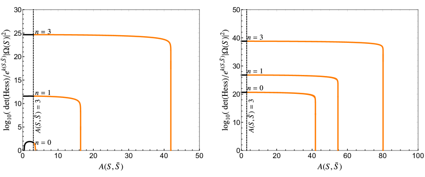
Figure 3: Determinants of the Kähler modulus block of the Hessian at $T=i$ with $(m,n)=(0,n)$ and polynomials given by $\mathcal{P}(j(T))=1$ (left) and $\mathcal{P}(j(T))=1+j(T)$ (right). The orange segments correspond to dS vacua assuming a stabilized dilaton. The vertical asymptote indicates the point where the determinant crosses to negative values.

m = 1:

This value for $m$ is particularly intriguing because the potential at $T=i$ is positive for $\Omega(S)\neq 0$ and does not depend on $A(S,\bar{S})$:

$$V(S,\bar{S},i,-i)=\frac{2^{4n+13}\pi^{8n+17}e^{k(S,\bar{S})}}{49\times 3^{2n+3}5^{2n+2}\Gamma^{4}(1/4)}\lvert\Omega(S)\rvert^{2}\lvert\mathcal{P}(1728)\rvert^{2}\,.$$ (3.7)

The second derivatives read

$$\begin{split}\partial_{t/a}^{2}V\rvert_{T=i}=&\frac{2^{4n+12}\pi^{8n+17}e^{k(S,\bar{S})}}{5^{2n+2}3^{2n+2}49\Gamma^{4}(1/4)}\lvert\Omega(S)\rvert^{2}\lvert\mathcal{P}(1728)\rvert^{2}\\ &\times\left[3A(S,\bar{S})-2\pm\frac{\Gamma^{8}(1/4)}{192\pi^{4}}\!\left(\!55+72n+373248\,{\text{Re}\,}\!\!\left(\!\frac{\mathcal{P}^{\prime}(1728)}{\mathcal{P}(1728)}\!\right)\!\right)\!\right]\,,\end{split}$$ (3.8)

$$\partial_{t,a}^{2}V\rvert_{T=i}=\frac{2^{4n+15}\pi^{8n+13}e^{k(S,\bar{S})}\Gamma^{4}(1/4)}{5^{2n+2}3^{2n-2}49}\lvert\Omega(S)\rvert^{2}\lvert\mathcal{P}(1728)\rvert^{2}{\text{Im}\,}\!\!\left(\frac{\mathcal{P}^{\prime}(1728)}{\mathcal{P}(1728)}\right)\,,\quad$$ (3.9)

and requiring the eigenvalues of the Hessian to be positive leads to the condition

$$A(S,\bar{S})>\frac{2}{3}+\frac{\Gamma^{8}(1/4)}{576\pi^{4}}\left[55+72n+373248\bigg{\lvert}\frac{\mathcal{P}^{\prime}(1728)}{\mathcal{P}(1728)}\bigg{\rvert}\right]\,.$$ (3.10)

However, the dilaton derivative is

$$\partial_{S}V\rvert_{T=i}=\frac{2^{4n+13}\pi^{8n+17}\lvert\mathcal{P}(1728)\rvert^{2}}{49\times 3^{2n+3}5^{2n+2}\Gamma^{4}(1/4)}e^{k(S,\bar{S})}\bar{\Omega}(\bar{S})(\Omega_{S}+k_{S}\Omega)\,.$$ (3.11)

Discarding the $\Omega(S)=0$ Minkowski solution, the above indicates that stabilizing the dilaton actually forces us into a Class A extremum. Hence the case $m=1$ is never a dS vacuum at $T=i$, in agreement with the tree-level Kähler potential analysis in Gonzalo:2018guu .

3.2 Class B-2 Vacua: $T=\rho$

For $T=\rho$, we must set $n<2$ or else all extrema will be Minkowski due to the vanishing of $G_{4}(\rho)$. We again separate the discussion for the case of $n=0$ and $n=1$.

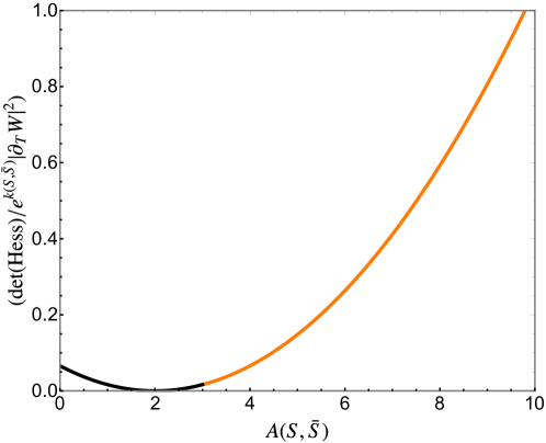
Figure 4: Rescaled Hessian determinant of the Kähler modulus block at $T=\rho$. Again the orange segments correspond to dS vacua assuming a stabilized dilaton.

n = 0 :

The value of the potential is then

$$V(S,\bar{S},\rho,\rho^{*})=\frac{4^{4m+6}\pi^{12m+12}e^{k(S,\bar{S})}}{3^{3m+3}1225^{m}\Gamma^{18}(1/3)}\lvert\Omega(S)\rvert^{2}\lvert\mathcal{P}(0)\rvert^{2}\left(A(S,\bar{S})-3\right)\,,\quad$$ (3.12)

and the non-zero second order derivatives are

$$\partial_{t}^{2}V\rvert_{T=\rho}=\partial_{a}^{2}V\rvert_{T=\rho}=\frac{2^{8m+13}\pi^{12m+12}e^{k(S,\bar{S})}}{3^{3m+3}1225^{m}\Gamma^{18}(1/3)}\lvert\Omega(S)\rvert^{2}\lvert\mathcal{P}(0)\rvert^{2}\left(A(S,\bar{S})-2\right)\,,\quad$$ (3.13)

so that the Hessian in the $T$ sector is

$$\text{det}(\text{Hess})\rvert_{T=\rho}=(\partial_{t}^{2}V)^{2}\rvert_{T=\rho}\,.$$ (3.14)

Thus, we see that the determinant of the Hessian is always positive (assuming the dilaton is stabilized), and the eigenvalues are positive for $A(S,\bar{S})>2$. Hence, there is a dS minimum for $A(S,\bar{S})>3$. This is depicted in Fig. 4.

n = 1 :

As in the previous section, for this value of $n$ the potential is always positive and does not depend on $A(S,\bar{S})$:

$$V(S,\bar{S},\rho,\rho^{*})=\frac{4^{4m+6}\pi^{12m+14}e^{k(S,\bar{S})}}{3^{3m+5}5^{2m+2}49^{m}\Gamma^{6}(1/3)}\lvert\Omega(S)\rvert^{2}\lvert\mathcal{P}(0)\rvert^{2}\,.$$ (3.15)

Also as above, $\partial_{S}V\rvert_{T=\rho}\propto\Omega_{S}+k_{S}\Omega$ and so it is not possible to stabilize the dilaton with $A(S,\bar{S})>0$. On the other hand, the determinant of the Kähler modulus block of the Hessian is

$$\partial_{t}^{2}V\rvert_{T=\rho}=\partial_{a}^{2}V\rvert_{T=\rho}=\frac{2^{8m+7}\pi^{12m+14}e^{k(S,\bar{S})}}{5^{2m+2}1323^{m}\Gamma^{6}(-2/3)}\lvert\Omega(S)\rvert^{2}\lvert\mathcal{P}(0)\rvert^{2}\left(3A(S,\bar{S})-2\right)\,.$$ (3.16)

So long as $A(S,\bar{S})>2/3$, the Kähler modulus sector is stabilized. This scenario cannot give dS vacua, but it does yield an intriguing model for dilaton quintessence: if the dilaton has an initial field value such that $A(S,\bar{S})>2/3$, then as the dilaton runs towards weak coupling, the cosmological constant in Eq. 3.15 decreases but the compact dimensions are stabilized. Indeed if we assume that $\Omega(S)\sim\sum_{a}e^{-S/b_{a}}$ and the dilaton Kähler potential is $k(S,\bar{S})=-\ln(S+\bar{S})+\mathcal{O}(e^{-\sqrt{S}})$, then $A(S,\bar{S})$ grows with $S$ and the stability of $T$ is maintained. We leave a detailed study of the phenomenology and cosmology of this scenario to future studies.

3.3 Class B-3 Vacua: Into the Fundamental Domain

We now step away from the fixed points and proceed elsewhere in the fundamental domain of $\text{PSL}(2,\mathbb{Z})$. As mentioned above, the stability of Class B extrema away from the fixed points are in general difficult to analyze since the Hessian is not required to be block diagonal and a thorough analysis requires a full treatment of the dilaton sector. Our focus here will be a study on the nature of extrema in the Kähler modulus sector in the absence of a dilaton. We will comment on re-introduction of the dilaton at the end of the section.

It was previously conjectured Cvetic:1991qm that all extrema of the $T$ sector must lie on the union of the boundary points included in $\widetilde{\mathcal{F}}$ and the line $\text{Re}(T)=0$. The argument for this is that the scalar potential in Eq. 2.23 displays an additional $\mathbb{Z}_{2}$ symmetry by swapping $T\leftrightarrow-\bar{T}$. The line $\text{Re}(T)=0$ consists of fixed points under this $\mathbb{Z}_{2}$, while the other boundary points in $\widetilde{\mathcal{F}}$ are fixed by the combined actions of $\mathbb{Z}_{2}$ and $\text{PSL}(2,\mathbb{Z})$ transformations. Assuming smooth behavior on the union of these curves, the scalar potential is then extremized in at least one direction on the union of these curves. The conjecture utilizes this observation to posit that all extrema of the $T$ sector lie on the above union of curves.

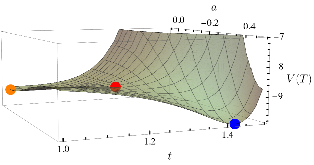
Figure 5: Potential with two minima and a saddle interpolating between them. The orange dot is a minimum at $T=i$, the blue dot is a minimum on the line $\text{Re}(T)=-\frac{1}{2}$, and the red dot signals the saddle point inside the fundamental domain.

We now argue that this is not the case. We will restrict ourselves to a simple parametrization of $H(T)$:

$$H_{1}(T)=\bigg{(}\frac{G_{4}(T)}{\eta^{8}(T)}\bigg{)}^{n}\bigg{(}\frac{G_{6}(T)}{\eta^{12}(T)}\bigg{)}^{m}(1+\beta\,j(T))\,.$$ (3.17)

We then extremize Eq. 2.23 with respect to $T$ and set $A(S,\bar{S})=0$. By scanning different values of $(m,n)\leq(5,5)$ and $\beta$, we found extrema for $\beta<10^{-2}$ throughout the fundamental domain. First, we find new saddle point extrema inside the fundamental domain. This can be expected, as once one has a minimum on the boundary and another minimum at one of the fixed points, an extremum must exist which interpolates between these points. We show an example of such situation in Fig. 5 where we have taken $(m,n)=(0,0)$ and $\beta=10^{-5}$ in Eq. 3.17. Second, we confirm the results of Novichkov:2022wvg : close to the fixed point $T=\rho$, and for $\mathcal{P}(j(T))=1$, there exists a minimum which tends to $T=\rho$ at increasing values of $m$. In Fig. 6 we show the first three concentric minima. Thus it appears that the conjecture in Cvetic:1991qm does not hold in general. However, this hints at the exciting possibility of a larger-than-anticipated modular landscape of heterotic vacua. We leave a thorough search for further vacua in the fundamental domain using general $H(T)$ to future studies.

Figure 6: Minima inside the fundamental domain close to the fixed point $T=\rho$ at varying $m$ and fixing $n=0$ in the function $H(T)$. The higher $m$, the closer the minimum is to the point $\rho$, which in this setup is a maximum and is represented by the blue dot. Each plot is appropriately rescaled.

Other than the above exceptional cases, we also found many minima that lie on the boundary points of $\widetilde{\mathcal{F}}$ and $\text{Re}(T)=0$. As anticipated by Theorem 1 and Corollary 1.2, all of the minima are AdS. However, in general, vacua away from the fixed points have non-vanishing values for $F_{T}$. Thus the criterion for positive vacuum energy in Class B-3 vacua is more relaxed as we only require:

$$A(S,\bar{S})>3-\frac{\widehat{V}(T,\bar{T})}{\lvert H(T)\rvert^{2}}\,.$$ (3.18)

A simple realization of the aforementioned modular landscape utilizing this condition can be seen in Fig. 7, where we give an example of an AdS minimum which is uplifted to dS once the requirement in Eq. 3.18 is met. Note that this does not destabilize the fixed point $T=\rho$, which remains a Minkowski minimum.

To truly confirm that Class B-3 dS vacua are possible, one must analyze the $S$ and $T$ sectors together. We have done this for several examples utilizing the framework on Shenker-like effects in the following section. We did not perform a general scan, but in principle it is indeed possible to stabilize Class B-3 vacua with positive vacuum energy utilizing the Shenker-like terms.

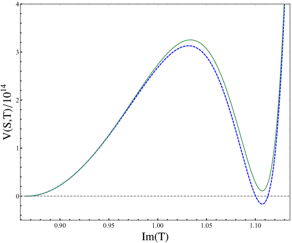
Figure 7: Potential for the parameters $\{\beta=10^{-3},\,m=2,\,n=2\}$. The AdS global minimum is located at $T=-0.5+1.107i$ while the fixed point $T=\rho$ is a Minkowski local minimum as expected from Section 3.2. When we turn the dilaton dependence on and $A(S,\bar{S})$ satisfies Eq. 3.18, the minimum in the outer rim becomes a dS local minimum, while $T=\rho$ stays a Minkowski minimum.

4 Non-Perturbative Stringy Effects & de Sitter Vacua

In the previous section, we described conditions on the function $A(S,\bar{S})$ such that the two-modulus potential could permit dS vacua. Traditional heterotic model building techniques do not furnish appropriate mechanisms – the use of $H_{3}$-flux or racetracks typically fix the dilaton vev in Class A vacua such that $\langle F_{S}\rangle=0$ and so $A(S,\bar{S})$ identically vanishes. Therefore, to either extend our no-go theorem or find dS vacua, we are naturally led to effects beyond gaugino condensation.

4.1 Class B de Sitter No-Go Theorem

In the above, we have seen that Class B extrema, with the assumption of a stabilized dilaton, can in principle have positive energy while stabilizing the Kähler modulus. However, this class of solutions is not a panacea – a broad subclass of Class B extrema are unstable in the dilaton subsector. A version of this statement can be found in deCarlos:1992kox , which we encapsulate and extend in the following no-go theorem:

Theorem 2.

At a point $(T_{0},S_{0})$, the scalar potential in Eq. 2.23 with
                $k(S,\bar{S})=-\ln(S+\bar{S})$ can not simultaneously satisfy:

1. $V(T_{0},S_{0})>0$

2. $\partial_{S}V(T_{0},S_{0})=0\quad\&\quad\partial_{T}V(T_{0},S_{0})=0$

3. $\widetilde{F}_{T}(T_{0})=0$

4. Eigenvalues of the Hessian of $V(T,S)$ at $(T_{0},S_{0})$ are all $\geq 0$.

Proof.

The proof proceeds in a similar fashion as the proof of Theorem 1. We assume (i)-(iv) are true and find a contradiction. To reconcile (i) and (iii), we must be in a Class B extrema such that Eq. 2.35 and its complex conjugate are satisfied. For (i) to be true, we also require that $H(T_{0})\equiv H_{0}\neq 0$ and we can once again introduce a parameter $\Lambda^{4}>0$ such that

$$V(T_{0},S_{0})=e^{k_{0}}Z_{0}\lvert H_{0}\rvert^{2}\Lambda^{4}\,.$$ (4.1)

Once again the subscript 0 denotes evaluation at $(T,S)=(T_{0},S_{0})$. This can be solved with

$$(\Omega_{S})_{0}=-(k_{S})_{0}\Omega_{0}\pm\sqrt{(k_{S\bar{S}})_{0}}\bigg{\{}\Lambda^{2}\pm i\bigg{(}\frac{3\lvert\Omega_{0}\rvert^{2}\lvert H_{0}\rvert^{2}-\lvert\Omega_{0}\rvert^{2}\widehat{V}_{0}}{\lvert H_{0}\rvert^{2}}\bigg{)}^{\frac{1}{2}}\bigg{\}}\,,\quad$$ (4.2)

where any of the four sign combinations are valid. Note that $k(S,\bar{S})$ is given its tree-level expression in the assumptions of the theorem but we keep it general for now. Similarly, $\widehat{V}_{0}$ vanishes by (iv) and we will set it to zero below. For the second condition in (ii), note that

$$\begin{split}\partial_{T}V(T,S)=e^{k}Z\lvert\Omega\rvert^{2}\bigg{\{}\bar{H}(A-3)\widetilde{F}_{T}+\partial_{T}\widehat{V}-\frac{3i}{2\pi}\widehat{G}_{2}\widehat{V}\bigg{\}}\,.\end{split}$$ (4.3)

Every term in the above derivative is proportional to $\widetilde{F}_{T}$ or its complex conjugate and so (iii) ensures the entire expression vanishes. By a similar logic, all mixed $S$ and $T$ derivatives vanish:

$$\partial_{S}^{k}\partial_{\bar{S}}^{l}\partial_{T}V(T_{0},S_{0})=0\quad\quad\forall\,\,k,\,l\in\mathbb{N}_{+}\,.$$ (4.4)

Hence the Hessian is block diagonal. We now examine the eigenvalues of the dilaton subsector. The components of the Hessian in terms of the fields $S=s+ib$ are

$$\partial_{s}^{2}V =2\partial_{S}\partial_{\bar{S}}V+2\text{Re}(\partial_{S}^{2}V)\,,\quad$$ (4.5)

$$\partial_{b}^{2}V =2\partial_{S}\partial_{\bar{S}}V-2\text{Re}(\partial_{S}^{2}V)\,,\quad$$ (4.6)

$$\partial_{s}\partial_{b}V =-2\text{Im}(\partial_{S}^{2}V)\,.$$ (4.7)

First, we see that the expressions for $\Omega_{S}(S_{0})$ and $\Omega_{SS}(S_{0})$ imply that

$$\partial_{S}\partial_{\bar{S}}V(T_{0},S_{0}) =\frac{e^{k_{0}}Z_{0}\lvert\Omega_{0}\rvert^{2}}{(k_{S\bar{S}})^{2}_{0}}\bigg{[}\left(2\lvert H_{0}|^{2}\lvert\Omega_{0}|^{2}+\Lambda^{4}\widehat{V}_{0}\right)(k_{S\bar{S}})^{3}_{0}$$ (4.8)

$$\,\qquad+\left((3-\widehat{V}_{0})\lvert\Omega_{0}\rvert^{2}+\Lambda^{4}\lvert H_{0}\rvert^{2}\right)\left(k_{S\bar{S}\bar{S}}k_{SS\bar{S}}-k_{S\bar{S}}k_{SS\bar{S}\bar{S}}\right)_{0}\bigg{]}$$

$$\rightarrow-\frac{2Z_{0}\lvert H_{0}\rvert^{2}(2\lvert\Omega_{0}\rvert^{2}+\Lambda^{4})}{(S_{0}+\bar{S}_{0})^{3}}\,.$$ (4.9)

In going to the second line we set $k(S,\bar{S})=-\ln(S+\bar{S})$ and $\widehat{V}(T_{0},\bar{T}_{0})=0$. Then by identical logic to Theorem 1, we see that at least one eigenvalue of the Hessian is negative. Logically speaking, we must supplement the assumptions of the theorem with $\text{Re}(S_{0})>0$, but this is a physical requirement for a sensible coupling constant. Thus (iv) is incompatible with (i)-(iii) and the theorem is demonstrated. ∎

In Appendix C we prove a similar statement to the above for orbifolds with non-trivial mixing in the Kähler potential displayed in Eq. 2.21. For the moment, we find an immediate corollary:

Corollary 2.1.

Extrema of the two-modulus model with $k(S,\bar{S})=-\ln(S+\bar{S})$
                    and Eq. 2.18 can never be dS vacua at the fixed points of $\text{PSL}(2,\mathbb{Z})$.

This follows from Theorems 1 and 2 and the fact that $\widetilde{F}_{T}$ vanishes at the $\text{PSL}(2,\mathbb{Z})$ fixed points for all cases except for $(m,n)=(1,n)$ at $T=i$ and $(m,n)=(m,1)$ at $T=\rho$ – see Appendix A. However, as discussed in Section 3, these cases can only ever yield unstable dS and the corollary is verified.

Thus we have an analytic argument for further results of Gonzalo:2018guu . They found by numerical analysis that Class B vacua at the fixed points were never dS vacua in cases where $\Omega(S)$ was a sum of exponentials, which is reminiscent of a racetrack superpotential. We see that this result and more is captured by Corollary 2.1 – for a tree-level dilaton Kähler potential, no racetrack or other non-perturbative effect captured by $\Omega(S)$ in the superpotential can result in dS vacua at $T=i,\,\rho$. The same applies for $H_{3}$-flux appearing as an additive constant in $\Omega(S)$. This result is a natural extension of Quigley:2015jia to orbifold models with threshold corrections and worldsheet instantons.

Theorem 2 illustrates that not any Class B extremum can be a dS vacua – in particular, constructing arbitrarily complicated superpotentials via $\Omega(S)$ is insufficient. However, Eq. 4.8 indicates how to go beyond Theorem 2 at the fixed points – one must go beyond the tree-level Kähler potential for the dilaton. This can be achieved by the Shenker-like terms briefly described in the introduction. We now turn to reviewing and modeling these effects.

4.2 Stringy Effects in Heterotic Theories

As emphasized above, gaugino condensation is not an inherently stringy phenomenon – rather, it is a purely quantum field-theoretical effect. This is evident from the form of the non-perturbative superpotential in Eq. 2.16, which contributes terms to the Lagrangian of the form $\delta\mathcal{L}\sim e^{-1/g_{s}^{2}}$. Truly stringy non-perturbative effects would scale as $\delta\mathcal{L}\sim e^{-1/g_{s}}$, which can be found via D-branes in theories with open strings. Contributions from such stringy effects would be stronger than gaugino condensation at weak coupling.

Considering such effects in the context of heterotic models at first seems surprising, given that these string theories lack D-branes. Nonetheless, heterotic models can and do have these stringy non-perturbative effects. The original argument for the existence of such effects by Shenker Shenker:1990 is based on the scaling properties of matrix theory amplitudes and applies to all closed string theories.

Shenker made a generic existence argument, but one can go a bit further by leveraging string dualities Silverstein:1996xp ; Antoniadis:1997nz . Indeed, Silverstein Silverstein:1996xp extended these general arguments by outlining how such non-perturbative stringy effects could be seen from the dualities of heterotic theories with type I and type IIA string theories. Let us first consider the duality with type I. The $10d$ type I/heterotic map is

$$\begin{array}[]{rcl}G^{H}_{MN}&=&g_{s}^{H}G_{MN}^{I}\\ g_{s}^{H}&=&(g_{s}^{I})^{-1}\,,\end{array}$$ (4.10)

where $G_{MN}^{i}$ is the $10d$ metric of heterotic or type I theory. Thus, type I worldsheet instantons wrapping a 2-cycle with area $A^{I}$ that give contributions $\delta\mathcal{L}\sim e^{-A_{I}}$ get mapped to $\delta\mathcal{L}\sim e^{-A_{H}/g_{s}^{H}}$. This is precisely the type of Shenker-like effect described above.

On the type IIA side, one can consider a scenario where the heterotic dilaton is mapped to a Kähler modulus on the type IIA side: $S^{H}\leftrightarrow T^{IIA}$. Such a duality is known to hold also in $4d$ in the large volume/weak coupling limit Kachru:1995wm ; Vafa:1995gm . In this case, Silverstein considers “worldline” instanton contributions $\delta\mathcal{L}\sim\sum_{m}e^{-mr}$ arising from strings wrapping a non-contractible loop of radius $r$ in the compactification manifold. This implies that the compactification manifold must have a non-trivial fundamental group. Applying the duality, we get in the heterotic side an effect which again falls like $\delta\mathcal{L}\sim\sum_{m}e^{-m/g_{s}^{H}}$.

The above was made much more tangible via the explicit calculations in $10d$ and $9d$ heterotic string theories by Green and Rudra in Green:2016tfs . The authors calculated one-loop diagrams in the Hořava-Witten background of $11d$ supergravity and find non-trivial $R^{4}$ terms which can be cast as contributions in the heterotic action proportional to $e^{-1/g_{s}}$. For example, a one-loop $4$ graviton bulk amplitude contributes a term to the $10d$ Spin$(32)/\mathbb{Z}_{2}$ heterotic effective action of the form

$$S^{HO}\supset\frac{g_{HO}^{-1/2}}{2^{8}(2\pi)^{7}4!\,l_{H}^{2}}\int_{\mathcal{M}_{10}}\sqrt{-G}\,t_{8}t_{8}R^{4}\mathbf{G}_{3/2}(ig^{-1}_{HO})\,,\quad$$ (4.11)

where $t_{8}$ is a rank-eight tensor and $l_{H}$ is the heterotic string length. The dependence on the string coupling $g_{HO}$ is encoded in the real-analytic Eisenstein series $\mathbf{G}_{s}(\tau)$. These are non-holomorphic modular forms with weight $(0,0)$ (i.e. non-holomorphic modular functions) – see Appendix A. For $s=3/2$, the series has a small-$g_{s}$ expansion

$$\mathbf{G}_{3/2}(ig_{s}^{-1})\! =\zeta(3)g_{s}^{-3/2}+2\zeta(2)g_{s}^{1/2}+\sum_{n\in\mathbb{Z}^{+}}4\pi\sigma_{-1}(\lvert n\rvert)e^{-\frac{2\pi\lvert n\rvert}{g_{s}}}(1+\mathcal{O}(g_{s}))$$ (4.12)

$$=\zeta(3)g_{s}^{-3/2}+2\zeta(2)g_{s}^{1/2}+e^{-\frac{2\pi}{g_{s}}}\left(4\pi+\frac{3}{4}g_{s}+\mathcal{O}(g_{s}^{2})\right)+\mathcal{O}(e^{-\frac{4\pi}{g_{s}}})\,,$$ (4.13)

$\sigma_{s}(n)$ being the divisor sum, as defined in Appendix A. Thus we see that there is an infinite set of non-perturbative instanton contributions of the form predicted by Shenker Shenker:1990 . This contribution to the action is not unlike the $R^{4}$ term in type IIB string theory, where the $g_{s}^{-1}$ dependence is augmented to a dependence on the axio-dilaton. Indeed one can think of the result in Eq. 4.11 as being related to the $9d$ $R^{4}$ term in IIB via orientifold projection to type I, S-dualizing to HO, and then taking the $10d$ limit. The authors find a similar structure in the gauge sector via a non-perturbative contribution to the $F^{4}$ correction to the effective action. Interestingly, Green:2016tfs find these instanton effects for both heterotic string theories in $9d$, but the calculated Shenker-like effects vanish in the $10d$ limit of the $E_{8}\times E_{8}$ heterotic string. This makes a tantalizing connection with the discussion of stable open heterotic strings by Polchinski Polchinski:2005bg .

We close this discussion with a note on the importance of duality in the above results for the heterotic Shenker-like terms in $9d$ and $10d$. As argued in Green:2016tfs , S-duality between type I and HO cannot operate term-by-term in Eq. 4.11 – if we write the $R^{4}$ term of the $9d$ HO and type I theories as $r_{i}\ell_{i}^{-1}g_{i}^{-\frac{1}{2}}U(ig_{i}^{-1})t_{8}t_{8}R^{4}$ with $r_{i}$ the radius of the additional $S^{1}$, $\ell_{i}$ the string length, $g_{i}$ the string coupling, and $i=I,HO$, then S-duality demands

$$U(ig_{HO}^{-1})=U(ig_{I}^{-1})$$ (4.14)

since $r_{HO}\ell_{HO}^{-1}g_{HO}^{-\frac{1}{2}}=r_{I}\ell_{I}^{-1}g_{I}^{-\frac{1}{2}}$. This property is not satisfied by the perturbative part of the $R^{4}$ coefficient, indicating that one must include additional terms. On the other hand, it is satisfied by the real-analytic Eisenstein series – it follows from their invariance under S-transformations of $\text{PSL}(2,\mathbb{Z})$. Thus one could argue that heterotic Shenker-like effects play an important role in the duality web connecting string theories.

This exhausts the discussion of heterotic stringy non-perturbative effects in the literature, as far as the current authors are aware. Clearly, these effects are poorly understood and deserve thorough investigation in their own right. However, in the following section we will attempt to understand the impact of these effects on heterotic vacua in the effective $4d$ theories considered above and leave an explicit full-fledged derivation for future work. Along a similar vein, these Shenker-like effects have been previously applied to the program of heterotic particle phenomenology in the form of “Kähler Stabilized Models” Casas:1996zi ; Binetruy:1996nx ; Binetruy:1997vr ; Barreiro:1997rp ; Kaufman:2013pya – see Gaillard:2007jr for a review.

4.3 Stringy de Sitter Vacua & the Linear Multiplet Formalism

As argued above, heterotic string theories contain non-perturbative corrections to their effective actions with strength $\mathcal{O}(e^{-1/g_{s}})$. In the $4d$ models we have introduced, these corrections will appear in the Kähler potential of the low energy effective theory. To study the impact of these non-perturbative effects on the two-modulus model, we must settle for a parametrization in the absence of explicit calculations. For concrete calculations, we will assume that the Shenker-like terms are functions of solely the dilaton and therefore they have the characteristic strength of $\mathcal{O}(e^{-1/g_{4}})$. We will return to the question of Kähler modulus dependence at the end of this section. Furthermore, we follow the conventions of Gaillard:2007jr and use the linear multiplet formalism for the dilaton Ferrara:1974ac ; Siegel:1979ai . This has been advocated as the superior convention for the dilaton Derendinger:1994gx ; Gates:1988kp ; Siegel:1988qu since it naturally describes corrections to the gauge coupling, Green-Schwarz anomaly cancellation conditions Butter:2014eva ; Gaillard:2017ypo ; Gaillard:2019ofq , effective descriptions of gaugino condensation, and higher-genus corrections. The component fields of the linear multiplet superfield $L$ are a real scalar $\ell$ (the dilaton), a Majorana fermion $\psi$ (the dilatino), and an antisymmetric tensor (the 2-form $B_{2}$). This decomposition also motivates the linear multiplet formalism as the natural choice since its degrees of freedom are precisely those of the string compactification.

In the $U(1)_{K}$ superspace formalism Binetruy:2000zx , the kinetic contribution to the effective supergravity action is determined by the superspace integral

$$\mathcal{L}_{KE} =\int d^{4}\theta E(-2+f(L))\,,\quad$$ (4.15)

where $E$ is the supervielbein determinant. The function $f(L)$ parametrizes the Shenker-like terms described above. It is related to the dilaton “Kähler potential”

$$k(L) =\ln(L)+g(L)\,,\quad$$ (4.16)

via the differential equation

$$L\,\frac{df}{dL} =-L\,\frac{dg}{dL}+f\,.$$ (4.17)

In the presence of the non-perturbative terms, the relation between $g_{4}$ and the dilaton vacuum expectation value is altered:

$$\frac{g_{4}^{2}}{2}=\bigg{\langle}\frac{\ell}{1+f(\ell)}\bigg{\rangle}\,.$$ (4.18)

In the linear multiplet formalism, gaugino condensation does not induce a superpotential for the dilaton. Instead, the scalar potential of the Kähler modulus and dilaton model can be calculated from the corrections to the gauge kinetic function, as written in Eq. 2.12. See Gaillard:2007jr for details. If we consider a single condensing gauge group with beta function coefficient $b_{a}$ (corresponding to $\Omega(S)=e^{-S/b_{a}}$ in the chiral formalism of Section 2) the scalar potential of Eq. 2.23 in the linear multiplet formalism becomes

$$V(\ell,T,\bar{T})=Z(T,\bar{T})\bigg{[}\!\bigg{(}\frac{(1+b_{a}\ell)^{2}(1+\ell g^{\prime}(\ell))}{b_{a}^{2}\ell^{2}}-3\!\bigg{)}\lvert H(T)\rvert^{2}+\widehat{V}(T,\bar{T})\bigg{]}\ell e^{g(\ell)-(f(\ell)+1)/b_{a}\ell}\,.$$ (4.19)

For a single gaugino condensate, one can bypass superspace calculations and derive this potential simply by taking Eq. 2.23 and implementing the tree-level relation between chiral and linear multiplet formalisms:

$$\frac{\ell}{1+f(\ell)}=\frac{1}{S+\bar{S}}\,.$$ (4.20)

To proceed, we must specify the functions $f(\ell)$ and $g(\ell)$ that parameterize the non-perturbative stringy terms. Due to the differential equation in (4.17), we need only specify one of the functions and a boundary condition. As in Gaillard:2007jr , we will specify $f(\ell)$ and fix $g(\ell)$ by the requirement that $g(0)=0$. This last condition is simply demanding that the non-perturbative effects vanish as the string coupling vanishes and only gets rid of a constant in the solution for $g(\ell)$. Note that one could also specify $g(\ell)$ and then derive $f(\ell)$. We take $f(\ell)$ to have the form Gaillard:2007jr

$$f(\ell)=\sum_{n=0}A_{n}\ell^{q_{n}}e^{-B/\sqrt{\ell}}\,,\quad$$ (4.21)

with constants $A_{n}$, $q_{n}$, and $B$. We will always consider $B>0$ with the expectation that non-perturbative effects should vanish at exponentially at large field values Witten:1996bn . The polynomial in $\ell$ is mirroring the structure of the real-analytic Eisenstein series expansion in Eq. 4.13. The above is essentially a parametrization for the first term in the infinite series of Eq. 4.13. In principle, we should include these higher order instantons. In practice, if our vacuum yields a small value for the first instanton, we will neglect higher order terms. We will return to this point below.

With this parametrization of $f(\ell)$, $g(l)$ is

$$g(\ell) =\sum_{n=0}A_{n}B^{2q_{n}}\bigg{\{}2(1-q_{n})\Gamma(-2q_{n},B/\sqrt{\ell})-\Gamma(1-2q_{n},B/\sqrt{\ell})\bigg{\}}\,,\quad$$ (4.22)

where $\Gamma(a,x)$ is the upper incomplete gamma-function

$$\Gamma(s,x)=\int_{x}^{\infty}y^{s-1}e^{-y}dy\,.$$ (4.23)

We now consider specific examples of Eq. 4.19 using Eq. 4.21 and Eq. 4.22. To simplify the discussion, we will consider vacua at the fixed point $T=\rho$. So long as $n=0$ in the parametrization of $H(T)$, Eq. 2.19, any dS minimum in the dilaton sector is immediately a minimum of the $T$ sector. Furthermore, $\widehat{V}(T,\bar{T})$ in Eq. 4.19 vanishes. We can also set $m=0$ without loss of generality since non-zero $m$ simply modulates the value of the vacuum energy via an overall factor in Eq. 4.19.

Example 1: Trivial polynomial

First, we consider the case of a trivial polynomial setting $q_{n}=0$ $\forall$ $n$:

$$f_{1}(\ell) =A_{0}e^{-B/\sqrt{\ell}}\,,\quad$$ (4.24)

$$g_{1}(\ell) =A_{0}\bigg{\{}2\Gamma(0,B/\sqrt{\ell})-e^{-B/\sqrt{\ell}}\bigg{\}}\,.$$ (4.25)

If we take $B=\pi$ and $A_{0}=26$, we find the potential on the left-hand side of Fig. 8. At the dS vacuum, we find

$$g_{4} \simeq 0.99\,,\quad$$

$$\langle f(\ell)\rangle \simeq 1.92\,,\quad$$ (4.26)

$$\langle e^{-B/\sqrt{\ell}}\rangle \simeq 7.4\times 10^{-2}\,.$$

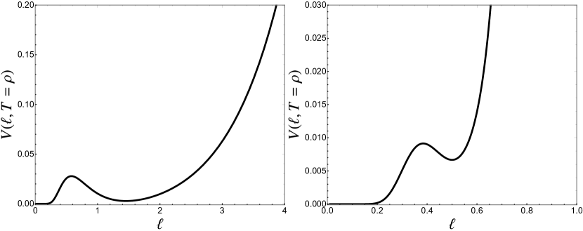
Figure 8: Plots of the scalar potential evaluated at $T=\rho$ for Example 1 (left) and Example 2 (right).

Examples 2 & 3: Non-trivial polynomials

Let us also consider two examples with non-trivial polynomials. We will keep the first two terms in Eq. 4.21:

$$f_{2,3}(\ell)=(A_{0}+A_{1}\ell^{q})e^{-B/\sqrt{\ell}}\,.$$ (4.27)

If we take $q=-0.5$, $B=2\pi$, $A_{0}=-7372$, and $A_{1}=7254$, we find the potential on the right in Fig. 8 At this minimum, the parameters take the values

$$g_{4} \simeq 0.84\,,\quad$$

$$\langle f(\ell)\rangle \simeq 0.39\,,\quad$$ (4.28)

$$\langle e^{-B/\sqrt{\ell}}\rangle \simeq 1.3\times 10^{-4}\,.$$

Instead, if we take $q=1/2$, $B=0.6\pi$, $A_{0}=10$, $A_{1}=9$

$$g_{4} \simeq 0.70\,,\quad$$

$$\langle f(\ell)\rangle \simeq 2.1\,,\quad$$ (4.29)

$$\langle e^{-B/\sqrt{\ell}}\rangle \simeq 0.11\,.$$

This final example is motivated by the Eisenstein expression from Green:2016tfs , where the polynomial coefficients are $\mathcal{O}(1-10)$. In both examples 2 and 3, the string coupling is stabilized close to the oft quoted phenomenological target of $g_{4}=2^{-1/2}\simeq 0.707$.

Let us make several comments on these vacua. First, note that the relationship between the linear and chiral multiplet formalisms in Eq. 4.20 implies that the typical dilaton runaway $\text{Re}(S)\rightarrow 0$ to weak coupling maps to $\ell\rightarrow 0$. Examination of the potentials in Fig. 8 shows that vacuum tunneling is possible via bubble nucleation to Minkowski space with $g_{s}\rightarrow 0$. This generic behavior of the vacua is rooted in the vanishing of the Shenker-like effects at weak coupling. Thus the dS vacua generated by Shenker terms are metastable. This is in accord with the general notion that if dS vacua exist in theories of quantum gravity, they must be at best metastable Goheer:2002vf and perhaps correspond to resonances Maltz:2016iaw ; Brahma:2020tak ; Bernardo:2021rul or mixed states in the AdS/CFT correspondence Kaloper:1999sm ; Hawking:2000da ; Freivogel:2005qh ; Maldacena:2010un .

Second, an important concern regarding the above vacua is control. Perturbative heterotic $4d$ string vacua which generate weakly-coupled non-abelian gauge groups with values of the gauge couplings roughly of that of simple GUTs $\alpha_{\rm GUT}\simeq 1/25$ cannot exist at large volume ${\cal V}$ of the compactification manifold. This statement follows from the tree-level relation between the value of the tree-level heterotic $4d$ gauge coupling $\alpha_{4d}$, the $4d$ heterotic dilaton $\text{Re}(S)$, the string coupling $g_{s}$, and the volume ${\cal V}$ of the extra dimensions

$$\alpha_{4d}^{-1}=4\pi\text{Re}(S)=\frac{\cal V}{g_{s}^{2}}\,.$$ (4.30)

If we now require $\alpha_{4d}^{-1}\simeq\alpha_{\rm GUT}^{-1}\simeq 25$ and $g_{s}<1$ to keep the heterotic string perturbative, this implies small compactification volume ${\cal V}<25$. Hence, the control mechanism of a large-volume expansion traditionally employed in the context of type IIB string vacua is not operational here.

Instead, four-dimensional heterotic strings, on orbifolds in particular, allow for the computation of perturbative and non-perturbative quantum corrections to the space-time effective action directly using worldsheet conformal field theory techniques. These corrections in turn are highly constrained by holomorphy and modular invariance, leading to a level of control (in some cases to infinite order of a particular series of quantum corrections) that can match and sometimes even surpass the level of large-volume expansion control in type IIB string vacua.

While the dilaton has been stabilized such that $g_{s}$ is in a perturbative regime, our parametrization of the Shenker-like effects in Eq. 4.21 ostensibly includes only the lowest order term in an infinite sum of non-perturbative terms. One would imagine that the full set of Shenker-like corrections has the form

$$f(\ell)=\sum_{\alpha=0}^{\infty}P_{\alpha}(\ell)e^{-B_{\alpha}/\sqrt{\ell}}\,,\quad$$ (4.31)

for some polynomials $P_{\alpha}(\ell)$ and constants $B_{\alpha}$. Indeed this is what the M-theory calculations of Green:2016tfs and duality arguments in Silverstein:1996xp point towards. Viewed from this perspective, consistency of the vacua requires that the high-order terms must be subdominant to the lowest-order one we have included. There are two ways this could be achieved, depending on the nature of the sum in Eq. 4.31. If the sum behaves similar to an instanton sum from Gopakumar-Vafa invariants, then the coefficients of the terms in Eq. 4.31 could grow rapidly as $\alpha$ increases. Control then demands that the exponentials decay rapidly with $\alpha$. Such a scenario would correspond to Example 2, where the ratio of the lowest-order exponential to the nominal value of the next exponential is $\langle e^{-2B/\sqrt{\ell}}/e^{-B/\sqrt{\ell}}\rangle=\langle e^{-B/\sqrt{\ell}}\rangle=\mathcal{O}(10^{-4})$. On the other hand, it may be that the coefficients in Eq. 4.31 do not grow rapidly, or at all, with $\alpha$. This would occur if the sum in Eq. 4.31 descends from a function such as the real-analytic Eisenstein series of Green:2016tfs . For such a scenario, control could be achieved with even modestly small exponentials, such as Example 3 above where the instanton ratio is only $\mathcal{O}(10^{-1})$. In either case, control hinges on the precise nature of the sum of Shenker-like terms. We are not in a position to argue generalities about this sum and leave a detailed discussion to future work.

Finally, we have downplayed the role of the Kähler modulus in this section and simply fixed $T=\rho$ at the very start. This approach is valid solely because of the remarkable number-theoretic properties of the scalar potential. Modular symmetry provides a simple means to identify critical points and vacuum criteria via the block-diagonal structure of the Hessian at $\text{PSL}(2,\mathbb{Z})$ fixed points. As shown in Section 3.2, $T$ is stabilized at $T=\rho$ if $A(S,\bar{S})>2$ – a condition that can, in principle, be satisfied by the Shenker-like terms.

On the other hand, we have parametrized the Shenker-like terms solely as a function of the dilaton. However, it is conceivable that these stringy effects depend on the Kähler modulus. While this would complicate the above calculations, there is a conceptual issue as well – an arbitrary dependence on the Kähler modulus would break the modular symmetry of $T$ and hence T-duality, which would raise concerns over the consistency of the string models. Therefore, we posit that the Shenker-like terms must uphold T-duality and consider three scenarios for the sum of non-perturbative effects:

• Case 1: the stringy effects do not depend on the Kähler modulus at all

• Case 2: the stringy effects depend on $T$ only through a modular invariant function

• Case 3: a single instanton term breaks T-duality, but the sum of instantons is a function with well-defined modular properties.

We argue that all the scenarios above may be realized in varied heterotic compactifications. For Case 1, the schematic calculations of Silverstein:1996xp indicate that the type IIA-heterotic map results in Shenker-like terms that do not depend on the Kähler modulus, although they may depend on other moduli that we have omitted in the considerations of this paper.

The second case above occurs in $4d$, $\mathcal{N}=2$ type IIB-heterotic dualities Candelas:1993dm ; Kachru:1995wm ; Kachru:1995fv . One example is type IIB on the mirror dual of $\mathbb{P}^{4}_{11226}[12]$, which is dual to heterotic on $K3\times T^{2}$. One combination of the type IIB complex structure moduli, $x$, gets mapped to the heterotic $T^{2}$ Kähler modulus via the j-invariant:

$$x=\frac{1728}{j(T)}+\cdots\,.$$ (4.32)

The dots are corrections that arise away from the strict heterotic weak coupling limit. Proposals for dualities involving similar type IIB-heterotic maps to the above but with hauptmoduls of congruence subgroups of $\text{PSL}(2,\mathbb{Z})$ were studied in Klawer:2021ltm ; Alvarez-Garcia:2021mzv .

The third possibility would be realized if the instanton sum was itself the expansion of some modular-invariant function, such as the real-analytic Eisenstein series in Eq. A.14 and similar to the results of Green:2016tfs . A single term in the sum breaks modular invariance, but the entire sum is invariant.

Let us reconsider our vacua in light of these scenarios for the sum of Shenker-like terms. First, since T-duality is preserved, the scalar potential remains a modular function, and so the fixed points of $\text{PSL}(2,\mathbb{Z})$ remain extrema of the scalar potential. Furthermore, $K_{T}$ retains its tree-level value at the fixed points since the $T$ derivative of the Shenker-like term sum must vanish at the fixed points. This implies that in almost all cases $F_{T}$ still vanishes at the fixed points. Thus, the condition $A(S,\bar{S})>3$ for a dS vacuum remains unchanged, except that $A(S,\bar{S})$ is now $T$ dependent and should be evaluated at the fixed point. Statements on the Hessian are much more difficult without a specific form of the Shenker-like terms. Modular symmetry implies that mixed entries in the Hessian vanish and we retain a block-diagonal structure. Beyond this, conditions for a minimum are dependent on the precise form of the Shenker-like terms.

We also note that for some of the vacua inside the fundamental domain, the hierarchy between the dilaton an Kähler modulus mass scales can become so large that the $T$-dependence of the Shenker-like terms becomes irrelevant. This is because at the level of dilaton stabilization, $T$ becomes frozen and rigidly stabilized at a much higher mass scale. In such vacua the Shenker-like terms become effectively purely dilaton-dependent. We have exhibited in Fig. 6 one class of vacua with this behavior. The $(m,n)=(m,0)$ with $P(j(T))=1$ vacua depicted there show stabilization of the Kähler modulus and its axion in ‘needle-thin’ vacua indicating the very high mass scale of $T$ far above the mass scale where $S$ (or $\ell$, respectively) gets stabilized.

We close this section with a comment on a puzzle posed in Silverstein:1996xp . As discussed above, obtaining the heterotic Shenker-like terms from duality with type IIA requires a non-trivial fundamental group on the IIA compactification manifold giving rise to worldline instantons. Similarly, one could examine type I-heterotic duality with a non-trivial fundamental group. Using the map defined above, one finds that worldline instantons on the type I side get mapped to heterotic terms of strength $\delta\mathcal{L}\sim\exp(-R/\sqrt{g_{s}})$, with $R$ the radius of the non-contractible loop. Assuming such contributions are not identically zero, they may be stronger at weak coupling than those predicted by Shenker. We have not included these Silverstein-like effects in our considerations and leave their explicit study and impact on heterotic vacua to future work.

5 Discussion

In this work, we have explored the possibility of extending dS no-go results to include non-perturbative stringy effects in the context of heterotic compactifications, particularly toroidal orbifolds. Focusing on the class of models where the light moduli consist of the dilaton and the overall Kähler modulus, we partially achieved this goal for extrema where the dilaton F-term vanishes via Theorem 1. The assumptions of this theorem are that the stringy effects are solely functions of the dilaton and that the superpotential has a factorized form and respects T-duality. The no-go theorem then rules out dS vacua arising from non-perturbative effects in both $T$ and $S$ in the superpotential and in $S$ in the Kähler potential when $\langle F_{S}\rangle=0$. As corollaries we were able to confirm previous conjectures and numerical studies arguing against dS vacua in the pure Kähler modulus theory and in the two-modulus theory when the dilaton Kähler potential has its tree-level expression. Other partial no-go theorems in the literature extend this to include perturbative quantum corrections in the heterotic moduli Kähler potential.

Theorem 2 utilizes a similar argument to Theorem 1 and forbid dS vacua at the fixed points of $\text{PSL}(2,\mathbb{Z})$ when the dilaton has only a tree-level Kähler potential, even if $\langle F_{S}\rangle\neq 0$. This rules out dS vacua arising purely from non-perturbative effects in the superpotential in $S$ and $T$ at the fixed points, again affirming a previous conjecture. Theorem 3 in Appendix C proves a kindred statement for the case of non-vanishing Green-Schwarz coefficient $\delta_{GS}$.

The above results point to non-perturbative corrections to the Kähler potential that yield $\langle F_{S}\rangle\neq 0$ as almost the only loophole to realize heterotic de Sitter vacua. After reviewing arguments in the literature in favor of universally present non-perturbative corrections to $\mathcal{K}$ at ${\cal O}(e^{-1/g_{s}})$, we demonstrated that the inclusion of these effects for heterotic orbifold vacua could lead to dilaton stabilization with F-term SUSY breaking in the dilaton sector using just a single gaugino condensate contribution in both AdS and metastable dS vacua where the Kähler modulus is stabilized as well, as emphasized in the models of Casas:1996zi ; Binetruy:1996nx ; Binetruy:1997vr ; Barreiro:1997rp ; Kaufman:2013pya ; Gaillard:2007jr . Furthermore, we showed that this stabilization could also lead to heterotic dS vacua. These solutions, if they truly exist vis a vis the ${\cal O}(e^{-1/g_{s}})$ Kähler corrections in a bona fide heterotic string construction, thread the needle through several partial no-go results – the no-go theorems we present here as well as those of Maldacena:2000mw ; Gautason:2012tb ; Green:2011cn ; Kutasov:2015eba ; Quigley:2015jia ; Gonzalo:2018guu .

These considerations leave a pressing open problem – determination of the precise form of the dilaton-dependent ${\cal O}(e^{-1/g_{s}})$ corrections to the Kähler potential, whose existence in the heterotic string so far is based on duality arguments and $11d$ computations. Aside from providing a potential mechanism to stabilize the dilaton and realize heterotic de Sitter vacua, these corrections are interesting in their own right as a window into truly stringy features of heterotic theories. A primary goal of future investigations will be to illuminate the nature of heterotic Shenker-like effects and to perform calculations to complement those of Green:2016tfs .

Along this analysis we reviewed how modular invariance of $4d$ heterotic orbifolds is maintained by an interplay of anomaly cancellation and 1-loop threshold corrections to the gauge kinetic function of the $4d$, ${\cal N}=1$. These corrections produce the leading $1/\eta^{6}(T)$ dependence of the gaugino condensate superpotential required by modular invariance. Further corrections in $T$ arise beyond leading order as effectively an infinite series of worldsheet instanton corrections constrained by modular invariance to resum into a product of integer powers of the holomorphic Eisenstein functions $G_{4}$ and $G_{6}$, and an arbitrary polynomial of the modular invariant $j$-function. We demonstrate in detail that for even simple non-trivial choices of these corrections there exist non-trivial SUSY breaking AdS vacua and critical points in the fundamental domain of the Kähler modulus $T$ away from its boundaries. This invalidates a long-standing conjecture that such critical points were to exist only on the boundary of the fundamental domain.

It is clear that based on these results there are several immediate directions for future work. Beyond the obvious task of establishing precise calculations for the form of the ${\cal O}(e^{-1/g_{s}})$ Kähler corrections, the structure of the modular invariant $T$-dependent non-perturbative corrections in the superpotential seems to foretell the existence of a whole landscape of SUSY breaking AdS vacua inside the $T$-fundamental domain. Determining the structure of this landscape as well as their potential upliftability to dS is a further task for future work. See also Mourad:2016xbk ; Basile:2018irz ; Baykara:2022cwj for non-SUSY heterotic AdS vacua.

Another straightaway question would be to include the presence of Wilson lines on heterotic orbifolds, as these are often used in breaking the heterotic gauge symmetry down to acceptable MSSM-like particle physics sectors. Including discrete Wilson lines typically breaks $\text{PSL}(2,\mathbb{Z})$ modular invariance down to congruence subgroups, which would affect the gaugino condensate-induced superpotential and thereby the vacuum structure of the theory. We leave a thorough study of these cases as yet another task for future work. On a wider scope, generalizing our results to several Kähler moduli and the inclusion of the complex structure moduli of orbifolds immediately calls for extending modular invariance beyond $\text{PSL}(2,\mathbb{Z})$ to e.g. SP$(4,\mathbb{Z})$ and more general automorphic groups which promise a landscape of heterotic vacua with an even richer number-theoretical structure.

Finally, on the more phenomenological side, the structure of the scalar potential connecting the Minkowski and dS vacua achievable by stabilizing the dilaton with ${\cal O}(e^{-1/g_{s}})$ Kähler corrections in $F_{S}$-SUSY-breaking vacua at the $T$-self dual points, indicates the presence of potentially slow-roll flat saddle points. As these might innately be suitable for constructing slow-roll inflation in these stabilized heterotic vacua, and string inflation setups within heterotic string vacua are mostly unknown, we leave this, too, as a well-motivated task for the future.

Appendix A Modular Symmetry & Forms

Here we collect some basic facts and identities on modular forms relevant for the results and arguments of the main text. For further details, see 123ModForms .

A.1 Basics & Definitions

As stated in the main text, the correct duality group of the Kähler modulus is $\text{PSL}(2,\mathbb{Z})=\text{SL}(2,\mathbb{Z})/\{\pm\mathds{1}\}$ since the elements $\gamma\in\text{SL}(2,\mathbb{Z})$ and $-\gamma\in\text{SL}(2,\mathbb{Z})$ define the same transformation for $T$ in Eq. 2.1. The generators of $\text{PSL}(2,\mathbb{Z})$ are

$$\mathcal{S}=\left(\begin{array}[]{cc}0&1\\ -1&0\end{array}\right)\,,\quad\mathcal{T}=\left(\begin{array}[]{cc}1&1\\ 0&1\end{array}\right)\,.$$ (A.1)

Using these generators, one can show that $T=i$ is stabilized by the order 2 cyclic subgroup $\{1,\mathcal{S}\}$ and $T=e^{2\pi i/3}\equiv\rho$ is invariant under the action of the order 3 cyclic subgroup $\{1,\mathcal{S}\mathcal{T},(\mathcal{S}\mathcal{T})^{2}\}$.

A modular form of weight $(p,q)$ is a function that transforms as

$$f(T,\bar{T})\rightarrow f(\gamma\cdot T,\gamma\cdot\bar{T})=(cT+d)^{p}(c\bar{T}+d)^{q}f(T,\bar{T})\,.$$ (A.2)

A particular subclass are holomorphic modular forms with weights $(p,0)$. We give our conventions for these in terms of the nome $q=e^{2\pi iT}$.

• j-invariant

  $$\begin{split}j(T)=&\frac{1}{q}+744+196884q+21493760q^{2}+864299970q^{3}\\ &+20245856256q^{4}+333202640600q^{5}+\cdots\end{split}$$ (A.3)

• Modular Discriminant
  Is the weight $(12,0)$ cusp form

  $$\Delta(T)=\eta^{24}(T)\,,\quad$$ (A.4)

  where the Dedekind eta is

  $$\eta(T)=q^{1/24}\prod_{n=1}^{\infty}(1-q^{n})\,.$$ (A.5)

  Note that the transformation property of the Dedekind eta is

  $$\eta(\gamma\cdot T)=\varepsilon(\gamma)(cT+d)^{\frac{1}{2}}\eta(T)\,.$$ (A.6)

  The multiplier system is a $24$-th root of unity and is given in terms of the Rademacher phi function $\Phi(\gamma)$:

  $$\varepsilon(\gamma)=\exp\bigg{[}\frac{2\pi i}{24}\Phi(\gamma)-\frac{i\pi}{4}\bigg{]}\,.$$ (A.7)

  For more explicit formulae, see DHoker:2022dxx .

• Holomorphic Eisenstein Series
  For $k>1$, the weight $(2k,0)$ holomorphic Eisenstein series are

  $$G_{2k}(T)=\sideset{}{{}^{\prime}}{\sum}_{c,d\in\mathbb{Z}}\frac{1}{(cT+d)^{2k}}=\zeta(2k)\sum_{(c,d)=1}\frac{1}{(cT+d)^{2k}}=\zeta(2k)E_{2k}(T)\,,\quad$$ (A.8)

  where the prime indicates that we omit $c,\,d=0$. Our conventions here differ from the mathematics literature by a factor of $2$. These have the Fourier development

  $$G_{2k}(T)=2\zeta(2k)\bigg{(}1-\frac{4k}{B_{2k}}\sum_{n=1}^{\infty}\sigma_{2k-1}(n)q^{n}\bigg{)}\,,\quad$$ (A.9)

  with the divisor sigma

  $$\sigma_{a}(n)=\sum_{d|n}d^{a}\,,\quad$$ (A.10)

  where $d|n=$ “$d$ divides $n$”. The exceptional case is $G_{2}(T)$, which is a quasi-modular form that transforms as

  $$G_{2}(\gamma\cdot T)=(cT+d)^{2}G_{2}(T)-2\pi ic(cT+d)\,.$$ (A.11)

  Then one can define a non-holomorphic Eisenstein series with weight $(2,0)$ as

  $$\widehat{G}_{2}(T)=G_{2}(T)+\frac{2\pi}{i(T-\bar{T})}\,.$$ (A.12)

  The quasi-modular form $G_{2}(T)$ and the Dedekind eta are related by

  $$\frac{d}{dT}\ln(\eta(T))=\frac{i}{4\pi}G_{2}(T)\,.$$ (A.13)

• Real Analytic Eisenstein Series:
  These are non-holomorphic modular forms of weight $(0,0)$. Similar to the series expression of the holomorphic Eisenstein series, we have

  $$\mathbf{E}_{s}(T) =\sum_{\gamma\in\Gamma_{\infty}\backslash PSL(2,\mathbb{Z})}\text{Im}(\gamma\cdot T)^{s}$$ (A.14)

  $$=t^{s}+\sum_{(c,d)=1,c\geq 1}\frac{t^{s}}{\lvert cT+d\rvert^{2s}}$$ (A.15)

  $$=\frac{1}{\zeta(2s)}\mathbf{G}_{s}(T)\,.$$ (A.16)

  The sum converges for $\text{Re}(s)>1$ and has a Fourier decomposition

  $$\mathbf{E}_{s}(T) =t^{s}+\frac{\Lambda(1-s)}{\Lambda(s)}t^{1-s}+\sum_{j=1}^{\infty}4\cos(2\pi ja)\frac{\sigma_{2s-1}(j)}{j^{s-\frac{1}{2}}\Lambda(s)}\sqrt{t}K_{s-\frac{1}{2}}(2\pi jt)\,,$$ (A.17)

  with $K$ is the modified Bessel function of the second kind and $\Lambda(s)=\pi^{-s}\Gamma(s)\zeta(2s)$ is a symmetrized version of the Riemann zeta function. The Fourier decomposition allows for a meromorphic continuation in the whole $s$ plane.

In general, the derivative of a modular form is not a modular form. However, one can define a covariant modular derivative utilizing $G_{2}(T)$. If $M_{2k}(T)$ is a weight $(2k,0)$ modular form, then

$$M_{2k+2}(T)=\partial_{T}M_{2k}(T)+\frac{k}{i\pi}G_{2}(T)M_{2k}(T)$$ (A.18)

is a weight $(2k+2,0)$ modular form. $G_{2}(T)$ is again exceptional, with

$$\widetilde{M}_{4}(T)=\partial_{T}G_{2}(T)-\frac{i}{2\pi}G_{2}^{2}(T)$$ (A.19)

defining a weight $(4,0)$ modular form. It is also possible to build non-holomorphic modular forms in a similar fashion. If $\widetilde{M}_{\kappa}(T)$ is a weight $(\kappa,0)$ modular form, then

$$\widetilde{M}_{\kappa+2}(T,\bar{T})=\partial_{T}\widetilde{M}_{\kappa}(T)+\frac{\kappa}{T-\bar{T}}\,\widetilde{M}_{\kappa}(T)$$ (A.20)

is a weight $(\kappa+2,0)$ non-holomorphic modular form. This is the method by which the scalar potential achieves modular invariance. There are several features of modular forms that are useful in searching for vacua:

• weight $(2k,0)$ modular forms vanish at $T=i$ for $k\in 2\mathbb{Z}+1$,

• weight $(2k,0)$ modular forms vanish at $T=\rho$ for $k\neq 0$ mod $3$.

These statements follow directly from the transformation properties of the modular forms as the behavior $\mathcal{S}\cdot i=i$ and $\mathcal{S}\mathcal{T}\cdot\rho=(\mathcal{S}\mathcal{T})^{2}\cdot\rho$. The case $k=1$ applies to the derivative of any modular function and implies that this derivative must vanish at the fixed points, as claimed in the main text for the derivative of Eq. 2.23.

A.2 Numerical Values

At the self-dual points, we have the values

$$\eta(i) =\frac{\Gamma\left(\frac{1}{4}\right)}{2\pi^{3/4}}$$ (A.21)

$$\eta(\rho) =e^{-\frac{i\pi}{24}}\frac{3^{1/8}\Gamma^{3/2}(1/3)}{2\pi}$$ (A.22)

and

$$j(i) =1728=12^{3}$$ (A.23)

$$j(\rho) =0$$ (A.24)

$$\partial_{T}j(i) =0$$ (A.25)

$$\partial_{T}j(\rho) =0\,.$$ (A.26)

The vanishing of $\partial_{T}j(T)$ is an avatar of the statements of weight $(2,0)$ forms above. Similarly, we immediately obtain

$$\widehat{G}_{2}(i,-i)=\widehat{G}_{2}(\rho,\bar{\rho})=0\,.$$ (A.27)

For the other Eisenstein series relevant for this paper, we have

$$G_{4}(i) =\frac{\Gamma^{8}(1/4)}{960\pi^{2}}$$ (A.28)

$$\partial_{T}G_{4}(i) =i\frac{\Gamma^{8}(1/4)}{480\pi^{2}}$$ (A.29)

$$G_{4}(\rho) =0$$ (A.30)

$$\partial_{T}G_{4}(\rho) =-i\frac{\Gamma^{18}(1/3)}{1280\pi^{7}}$$ (A.31)

and

$$G_{6}(i) =0$$ (A.32)

$$\partial_{T}G_{6}(i) =-i\frac{\Gamma^{16}(1/4)}{215040\pi^{5}}$$ (A.33)

$$G_{6}(\rho) =\frac{\Gamma^{18}(1/3)}{8960\pi^{6}}$$ (A.34)

$$\partial_{T}G_{6}(\rho) =i\sqrt{3}\,\frac{\Gamma^{18}(1/3)}{4480\pi^{6}}\,.$$ (A.35)

Thus for the function $H(T)$ in Eq. 2.19, we find

$$H(i) =\begin{cases}0&m>0\\ \frac{4^{n}\pi^{4n}}{15^{n}}\mathcal{P}(1728)&m=0\end{cases}$$ (A.36)

$$H_{T}(i) =\begin{cases}0&m>1\;\;\&\;\;m=0\\ -\frac{i}{7}2^{2n+1}15^{-n-1}\pi^{4n+4}\Gamma^{4}(1/4)\mathcal{P}(1728)&m=1\end{cases}$$ (A.37)

and

$$H(\rho) =\begin{cases}0&n>0\\ \left(\frac{16i}{35}\right)^{m}3^{-\frac{3m}{2}}\pi^{6m}\mathcal{P}(0)&n=0\end{cases}$$ (A.38)

$$H_{T}(\rho) =\begin{cases}0&n>1\;\;\&\;\;n=0\\ -i\left(\frac{16i}{7}\right)^{m}3^{-1-\frac{3m}{2}}5^{-m-1}e^{i\pi/3}\pi^{6m+1}\Gamma^{6}(1/3)\mathcal{P}(0)&n=1\end{cases}$$ (A.39)

The non-zero values of $H_{T}(T)$ at the fixed points may seem surprising at first glance given the argument above that the derivative of a modular function must vanish at the fixed points. However, recall that $H(T)$ is not strictly a modular function – it can transform with a non-trivial multiplier system. Instead, the expression $\partial_{T}\lvert H\rvert^{2}=\bar{H}H_{T}$ transforms as a proper weight $(2,0)$ non-holomorphic modular form and must vanish at the fixed points. Thus it must be that either $H(T)=0$ or $H_{T}(T)=0$ at $T=i,\,\rho$.

Appendix B Kähler Modulus Sector Expressions

B.1 General Condition For Theorem 1

In Theorem 1, we referenced an expression for $H_{TT}$ such that $\partial_{T}V(T,S)=0$ for $\widetilde{F}_{T}\neq 0$. The expression is

$$H_{TT}=\, \frac{3i}{2\pi}\bigg{\{}\widehat{G}_{2}\widetilde{F}_{T}+H\partial_{T}\widehat{G}_{2}+\widehat{G}_{2}H_{T}\bigg{\}}+\frac{\mathcal{K}_{TT\bar{T}}}{\mathcal{K}_{T\bar{T}}}\widetilde{F}_{T}$$ (B.1)

$$-\left(\frac{3i}{2\pi}\bar{H}\partial_{T}\bar{\widehat{G}}_{2}+\mathcal{K}_{T\bar{T}}\bar{H}\left(A(S,\bar{S})-3\right)\right)e^{2i\phi}\,,\quad$$ (B.2)

where we have suppressed arguments and defined re-scaled F-terms $\widetilde{F}_{T}=\eta^{6}\Omega^{-1}F_{T}$. The phase is given by $\phi=\text{arg}(\widetilde{F}_{T})$.

B.2 General dS Vacuum Conditions for $T=i$

Let us assume that the dilaton subsector is stabilized. By considering the most general case for the polynomial $\mathcal{P}(j(T))$, we have a dS minimum at $T=i$ when

$$\begin{array}[]{l}\lvert\mathcal{B}_{n}\rvert<1\,:\begin{cases}A(S,\bar{S})>2+\lvert\mathcal{B}_{n}\rvert\,\,\,\mbox{ if }\,\,\mathcal{R}_{n}>-\frac{192\pi^{4}}{\Gamma^{8}(1/4)}\lvert\mathcal{B}_{n}\rvert\\ \quad\quad\mbox{ or}\\ \mathcal{C}_{n}<A(S,\bar{S})<2-\lvert\mathcal{B}_{n}\rvert\,\,\,\mbox{ if }\,\,\mathcal{R}_{n}>\frac{192\pi^{4}}{\Gamma^{8}(1/4)}\lvert\mathcal{B}_{n}\rvert\\ \quad\quad\mbox{ or}\\ A(S,\bar{S})>\mathcal{C}_{n}\,\,\,\mbox{ if }\,\,-\frac{192\pi^{4}}{\Gamma^{8}(1/4)}<\mathcal{R}_{n}\leq-\frac{192\pi^{4}}{\Gamma^{8}(1/4)}\lvert\mathcal{B}_{n}\rvert\\ \quad\quad\mbox{ or}\\ A(S,\bar{S})<\mathcal{C}_{n}\,\,\,\mbox{ if }\,\,\mathcal{R}_{n}<-\frac{192\pi^{4}}{\Gamma^{8}(1/4)}\end{cases}\end{array}$$ (B.3)

$$\begin{array}[]{l}\lvert\mathcal{B}_{n}\rvert>1\,:\begin{cases}2-\lvert\mathcal{B}_{n}\rvert<A(S,\bar{S})<2+\lvert\mathcal{B}_{n}\rvert\,\,\,\mbox{ if }\,\lvert\mathcal{R}_{n}\rvert<\frac{192\pi^{4}}{\Gamma^{8}(1/4)}\lvert\mathcal{B}_{n}\rvert\\ \quad\quad\mbox{ or}\\ \mathcal{C}_{n}<A(S,\bar{S})<2+\lvert\mathcal{B}_{n}\rvert\,\,\,\mbox{ if }\,\,\mathcal{R}_{n}\geq\frac{192\pi^{4}}{\Gamma^{8}(1/4)}\lvert\mathcal{B}_{n}\rvert\\ \quad\quad\mbox{ or}\\ 2-\lvert\mathcal{B}_{n}\rvert<A(S,\bar{S})<\mathcal{C}_{n}\,\,\,\mbox{ if }\,\,\mathcal{R}_{n}<-\frac{192\pi^{4}}{\Gamma^{8}(1/4)}\lvert\mathcal{B}_{n}\rvert\end{cases}\end{array}$$ (B.4)

where we used the notation for $\mathcal{B}_{n}$ of Eq. 3.3 and we have also introduced

$$\mathcal{R}_{n}=1+8n+41472\,{\text{Re}\,}\!\left({\frac{\mathcal{P}^{\prime}(1728)}{\mathcal{P}(1728)}}\right)\,,\quad$$ (B.5)

$$\mathcal{C}_{n}\equiv\frac{2+\frac{\Gamma^{8}(1/4)}{192\pi^{4}}\,\mathcal{R}_{n}-\lvert\mathcal{B}_{n}\rvert^{2}}{1+\frac{\Gamma^{8}(1/4)}{192\pi^{4}}\,\mathcal{R}_{n}}\,.$$ (B.6)

If we assume $\mathcal{P}(1728)\in\mathbb{R}$, these conditions greatly simplify to

$$\begin{array}[]{lcl}2-\mathcal{B}_{n}<A(S,\bar{S})<2+\mathcal{B}_{n}&\quad\mbox{ for }&\mathcal{B}_{n}>1\,,\\ A(S,\bar{S})>2+\lvert\mathcal{B}_{n}\rvert&\quad\mbox{ for }&-1<\mathcal{B}_{n}<1\,,\\ 2+\mathcal{B}_{n}<A(S,\bar{S})<2-\mathcal{B}_{n}&\quad\mbox{ for }&\mathcal{B}_{n}<-1\,.\end{array}$$ (B.7)

Appendix C Orbifolds with $\delta_{GS}\neq 0$ & A Third No-Go Theorem

A natural question arises from the discussion in the main text – can the mixing of the moduli in the Kähler potential evade the theorems and result in dS vacua, even in the absence of Shenker-like terms? There is a natural basis for this mixing arising from anomaly cancellation, as described in Section 2. We now return to these orbifold models and prove a limited no-go result similar to Theorem 2.

We will utilize the chiral multiplet formalism where the dilaton is invariant under modular transformations. Our starting points are the superpotential Eq. 2.18 and the Kähler potential Eq. 2.6 using Eq. 2.21 so that

$$k(S,\bar{S},T,\bar{T})=-\ln\left(S+\bar{S}+\delta_{GS}\ln(-i(T-\bar{T})\lvert\eta(T)\rvert^{4})\right)+\delta k(S,\bar{S},T,\bar{T})\,.$$ (C.1)

Note that we have defined the dilaton-sector Kähler potential with the loop-corrected contribution and a function $\delta k(S,\bar{S},T,\bar{T})$, which we take to be a modular-invariant, non-holomorphic function that encodes non-perturbative effects such as the Shenker-like terms. The Green-Schwarz anomaly coefficient $\delta_{GS}$ should not be confused with $\delta k$. Similar to the main text, the F-terms read

$$F_{S} =\frac{H(T)}{\eta^{6}(T)}\bigg{(}\Omega_{S}+(-Y^{-1}+\delta k_{S})\Omega\bigg{)}\equiv\frac{H(T)}{\eta^{6}(T)}\widetilde{F}_{S}\,,\quad$$ (C.2)

$$F_{T} =\frac{\Omega(S)}{\eta^{6}(T)}\bigg{(}H_{T}-\frac{3i}{2\pi}\bigg{(}1+\frac{\delta_{GS}}{3Y}\bigg{)}H\widehat{G}_{2}+\delta k_{T}H\bigg{)}\equiv\frac{\Omega(S)}{\eta^{6}(T)}\widetilde{F}_{T}\,,\quad$$ (C.3)

where we have defined $Y=S+\bar{S}+\delta_{GS}\ln(-i(T-\bar{T})\lvert\eta(T)\rvert^{4})$. The Kähler metric is much more complicated than the cases found in the main text and we will not reproduce here. We write the scalar potential for these models as

$$\begin{split}V&=e^{k}Z(T,\bar{T})\bigg{\{}\lvert H\rvert^{2}\lvert\Omega\rvert^{2}(\widetilde{A}(S,T)-3)+\lvert\Omega\rvert^{2}\widehat{V}_{2}(S,T)\\ &\hskip 105.2751pt+H\bar{\Omega}\mathcal{K}^{S\bar{T}}\widetilde{F}_{S}\bar{\widetilde{F}}_{\bar{T}}+\bar{H}\Omega\mathcal{K}^{\bar{S}T}\bar{\widetilde{F}}_{\bar{S}}\widetilde{F}_{T}\bigg{\}}\,,\quad\end{split}$$ (C.4)

with $\widetilde{A}(S,T)=\lvert\Omega\rvert^{-2}\mathcal{K}^{S\bar{S}}\widetilde{F}_{S}\bar{\widetilde{F}}_{\bar{S}}$, $\widehat{V}_{2}(S,T)=\mathcal{K}^{T\bar{T}}\widetilde{F}_{T}\bar{\widetilde{F}}_{\bar{T}}$, and $Z(T,\bar{T})$ as defined in Eq. 2.26.

We now prove a no-go result similar to Theorem 2 of the main text. In particular, we demonstrate the impossibility of dS vacua at the fixed points of $\text{PSL}(2,\mathbb{Z})$ if the $\delta k$ contribution to the Kähler potential is discarded.

Theorem 3.

At the points $(T_{0}=i,S_{0})$ or $(T_{0}=\rho,S_{0})$, the scalar potential in Eq. C.4 defined via Eq. 2.18 and Eq. C.1 with $\delta k=0$ can not simultaneously satisfy:

1. $V(T_{0},S_{0})>0$

2. $\partial_{S}V(T_{0},S_{0})=0\quad\&\quad\partial_{T}V(T_{0},S_{0})=0$

3. Eigenvalues of the Hessian of $V(T,S)$ at $(T_{0},S_{0})$ are all $\geq 0$.

Proof.

First, we are considering the fixed points of $\text{PSL}(2,\mathbb{Z})$, so the requirement $\partial_{T}V(T_{0},S_{0})=0$ in (ii) is automatically satisfied. Furthermore, the Hessian is also block diagonal, so we can again consider the Kähler modulus and dilaton blocks individually. Second, recall from Appendix A that at the fixed points of $\text{PSL}(2,\mathbb{Z})$, the product $(\bar{H}H_{T})_{0}$ must vanish as a consequence of modular symmetry – $\partial_{T}\lvert H\rvert^{2}$ transforms as a weight $(2,0)$ modular form with trivial multiplier system. One can also observe this numerically from Eqs. A.36, A.37, A.38 and A.39. In almost all cases, the vanishing of this product occurs because $H_{T}=0$. This immediately implies that $\widetilde{F}_{T}=0$ since $\widehat{G}_{2}(T,\bar{T})$ must also vanish at the fixed points. However, cases where the integer pair $(m,n)$ in Eq. 2.19 correspond to $(1,n)$ or $(m,1)$ do not follow this pattern since they give $H_{T}\neq 0$ at $T=i,\,\rho$. Thus, we must divide our analysis into two cases. We will not consider the cases where $H=H_{T}=0$ at $T=i,\,\rho$ since these trivially give Minkowski extrema.

Case 1: $H(T_{0})\neq 0$
This is the case where $(\widetilde{F}_{T})_{0}=0$, so all positive contributions to the vacuum energy must come from the dilaton sector in the form of the function $\widetilde{A}(S,T)$ in Eq. C.4. Thus to satisfy (i), we require $(\widetilde{F}_{S})_{0}\neq 0$ & $(\mathcal{K}^{S\bar{S}})_{0}\neq 0$. We can again introduce a parameter $\Lambda$ such that

$$e^{k_{0}}Z_{0}\lvert H_{0}\rvert^{2}\lvert\Omega_{0}\rvert^{2}(\widetilde{A}_{0}-3)=e^{k}_{0}Z_{0}\lvert H_{0}\rvert^{2}\Lambda^{4}\,.$$ (C.5)

This can be solved to give

$$\Omega_{S}(S_{0})=Y_{0}^{-1}\Omega_{0}\pm(\mathcal{K}^{S\bar{S}}_{0})^{-1/2}\left(\Lambda^{2}\pm i\sqrt{3\lvert H_{0}\rvert^{2}}\right)\,.$$ (C.6)

Once again any of the four sign choices are valid. The first condition in (ii) is satisfied if

$$\Omega_{SS}(S_{0})=\frac{2\bar{\Omega}_{0}}{Y_{0}^{2}}\frac{(\bar{\widetilde{F}}_{\bar{S}})_{0}}{(\widetilde{F}_{S})_{0}}\,,\quad$$ (C.7)

where we have utilized the vanishing of $(\widetilde{F}_{T})_{0}$. Inserting the above expressions into $\partial_{S}\partial_{\bar{S}}V(S_{0},T_{0})$, we find

$$\partial_{S}\partial_{\bar{S}}V(S_{0},T_{0})=-\frac{2Z_{0}\lvert H_{0}\rvert^{2}(\Lambda^{4}+2\lvert\Omega_{0}\rvert^{2})}{Y_{0}^{3}}\,.$$ (C.8)

Note that $Y_{0}>0$ is required for a sensible value of the string coupling. Hence, by identical logic to Theorem 2, at least one eigenvalue in the dilaton block of the Hessian is negative and a (meta)stable dS vacuum is not possible for any function $\Omega(S)$.

Case 2: $H_{T}(T_{0})\neq 0$
Since it must be that $H_{0}=0$ for this case, the potential in Eq. C.4 simplifies greatly to

$$V_{0}=e^{k_{0}}Z_{0}\lvert\Omega_{0}\rvert^{2}(\widehat{V}_{2})_{0}\,.$$ (C.9)

Thus we must demand that $\Omega_{0}\neq 0$ to avoid a Minkowski extremum. Next, we note that

$$\partial_{S}V(S_{0},T_{0})=\frac{-(T_{0}-\bar{T}_{0})^{2}}{3Y_{0}+\delta_{GS}}Z_{0}\bar{\Omega}_{0}\lvert H_{T}\rvert^{2}_{0}\left((3Y_{0}+\delta_{GS})(\Omega_{S})_{0}-3\Omega_{0}\right)\,,\quad$$ (C.10)

after using the vanishing of $H_{0}$. Then to satisfy the first condition of (ii), the factor in parentheses must vanish and we obtain $(\Omega_{S})_{0}=3(3Y_{0}+\delta_{GS})^{-1}\Omega_{0}$. We now investigate the Kähler modulus block of the Hessian. Using the above, we see that

$$\partial_{T}\partial_{\bar{T}}V(S_{0},T_{0})=-\frac{2(3Y_{0}^{2}+\delta_{GS}Y_{0}+\delta_{GS}^{2})}{Y_{0}(3Y_{0}+\delta_{GS})^{2}}Z_{0}\lvert\Omega_{0}\rvert^{2}\lvert H_{T}\rvert^{2}_{0}\,.$$ (C.11)

Since both $Y>0$ and $\delta_{GS}>0$ Derendinger:1991hq , we see that $\partial_{T}\partial_{\bar{T}}V(S_{0},T_{0})<0$ and by the same logic used in Theorem 1 at least one of the eigenvalues of the Kähler modulus block of the Hessian is negative. ∎

From Theorem 3, we conclude that there is no non-perturbative contribution in the form of $\Omega(S)$ or $H(T)$ that can lift a fixed point extremum to a dS vacuum if $\delta k=0$, even for models with $\delta_{GS}\neq 0$. As discussed in the main text, if this additional term is included, dS vacua may be possible. If we again consider a fixed point $T_{0}$ of $\text{PSL}(2,\mathbb{Z})$ with $H(T_{0})\neq 0$, then Eq. C.4 is simply

$$V(S,T_{0})=e^{k}Z(T_{0},\bar{T}_{0})\lvert\Omega\rvert^{2}\lvert H(T_{0})\rvert^{2}(\widetilde{A}(S,T_{0})-3)$$ (C.12)

This is similar to the scenarios considered in the main text. We will not perform a thorough analysis here, but one could determine stability criteria for dS vacua at the fixed points and convert them into requirements on the Shenker-like terms encoded in $\delta k(S,\bar{S},T,\bar{T})$.

Appendix D Linear Multiplet Formalism & The Inverse Map

In this appendix, we develop a perturbative framework to invert the map between the linear multiplet formalism and the chiral multiplet formalism for the dilaton. With the Shenker-like terms corrections, we have the relation

$$\frac{\ell}{1+f(\ell)}=\frac{1}{S+\bar{S}}\,.$$ (D.1)

Our goal is to invert this relationship and write $\ell=\ell(s)$. Recalling the form of $f(\ell)$ used in Eq. 4.21

$$f(\ell)=\sum_{n}A_{n}\ell^{q_{n}}e^{-B/\sqrt{\ell}}\,,\quad$$ (D.2)

we see why the task is non-trivial – inversion requires us to solve a transcendental equation. We can make some progress in developing a perturbative approach. Let us work in the limit $\ell\ll 1$. Then the exponential dies out and to the lowest order we simply have $2s=\ell^{-1}$. To proceed, we want to develop a series

$$\ell=\frac{1}{2s}+\varepsilon y(s)+\cdots$$ (D.3)

where $\varepsilon$ is a small parameter controlling the expansion and $y(s)$ is some function of the dilaton to be determined. Unfortunately a brute force perturbative approach does not work – we cannot expand the exponential $e^{-B/\sqrt{\ell}}$ about $\ell=0$ since it has an essential singularity there. In the limit we are considering, $e^{-B/\sqrt{\ell}}$ is small, so our perturbative expansion should be based on the notion that

$$e^{-B/\sqrt{\ell}}\sim\mathcal{O}(\varepsilon)\,.$$ (D.4)

This would then imply that

$$\ell\sim\frac{B^{2}}{\ln^{2}(\varepsilon)}$$ (D.5)

to leading order. This is quite a peculiar setup, but intuitively it seems reasonable – if $\varepsilon$ is a small parameter, then $\ln^{-2}(\varepsilon)$ is also a small positive number. We are still performing a perturbative expansion, just one that involves a non-linear map of the expansion parameter. We formalize this observation by postulating a very general perturbative expansion

$$\begin{split}\ell&=\alpha\ell_{1}+\varepsilon^{a_{2}}\alpha^{b_{2}}\ell_{2}+\varepsilon^{a_{3}}\alpha^{b_{2}}\ell_{3}+\cdots\\ &=\alpha\ell_{1}+\delta\,,\quad\end{split}$$ (D.6)

where $\alpha=\ln^{-2}(\varepsilon^{a})$ and $a$ is unspecified for the moment. We also leave the powers in the higher order terms as variables to be solved. We now plug this into Eq. D.1, expand around $\delta=0$, and match powers of $\varepsilon$ and $\alpha$. For a sensible expansion, we must relate $\varepsilon$ to $s$. The natural guess from the discussion above is that

$$s=\ln^{2}(\varepsilon^{a})\,.$$ (D.7)

This also implies that the small parameters $\varepsilon$ and $\alpha$ are defined in terms of $s$ as

$$\varepsilon=e^{-\frac{\sqrt{s}}{a}}\,,\quad\mbox{where }\,\,\alpha=\frac{1}{s}\,.$$ (D.8)

To determine the value of $a$, we demand that

$$e^{-B/\sqrt{\ell_{1}}} =\varepsilon\,,\quad$$ (D.9)

$$\varepsilon^{\sqrt{\ell_{1}}Ba} =\varepsilon\,,\quad$$ (D.10)

so $a=\frac{\sqrt{\ell_{1}}}{B}$.

D.1 Example 1: Only $A_{0}\neq 0$

We explicitly solve the simple example where the series in Eq. 4.21 collapses to $f(\ell)=A_{0}e^{-B/\sqrt{\ell}}$. Then we have

$$2s =\ell^{-1}(1+A_{0}e^{-B/\sqrt{\ell}})$$ (D.11)

$$2\ln^{2}(\varepsilon^{a}) =(\alpha\ell_{1}+\delta)^{-1}(1+A_{1}e^{-B/\sqrt{\alpha\ell_{1}+\delta}})\,.$$ (D.12)

To leading order,

$$\begin{split}2\ln^{2}(\varepsilon^{a})&=\frac{\ln^{2}(\varepsilon^{a})}{\ell_{1}}\\ \ell_{1}&=\frac{1}{2}\,.\end{split}$$ (D.13)

Matching the next order yields

$$\begin{split}(a_{2},b_{2})&=(1,1)\\ \ell_{2}&=A_{0}\ell_{1}=\frac{A_{0}}{2}\end{split}$$ (D.14)

and following order is

$$\begin{split}(a_{3},b_{3})&=(2,1/2)\\ \ell_{3}&=\frac{A_{0}B\ell_{2}}{2\sqrt{\ell_{1}}}=\frac{A_{0}^{2}B}{2\sqrt{2}}\,.\end{split}$$ (D.15)

We then arrive at the series expansion

$$\begin{split}\ell&=\alpha\ell_{1}+\varepsilon\alpha\ell_{2}+\varepsilon^{2}\alpha^{1/2}\ell_{3}+\cdots\\ &=\frac{\ell_{1}}{s}+\frac{e^{-B\sqrt{s/\ell_{1}}}}{s}\ell_{2}+\frac{e^{-2B\sqrt{s/\ell_{1}}}}{s^{1/2}}\ell_{3}+\cdots\\ &=\frac{1}{2s}+\frac{A_{0}}{2s}e^{-B\sqrt{2s}}+\frac{A_{0}^{2}B}{2\sqrt{2s}}e^{-2B\sqrt{2s}}+\cdots\,.\end{split}$$ (D.16)

D.2 Example 2: $A_{0}$, $A_{1}\neq 0$

We now try the slightly harder example where $A_{0},A_{1}\neq 0$ and $q_{1}=-\frac{1}{2}$ in Eq. 4.21. We must then solve

$$2s=\ell^{-1}(1+(A_{0}+A_{1}\ell^{-1/2})e^{-B/\sqrt{\ell}})\,.$$ (D.17)

Much of our discussion from the previous example carries over – the only adjustment we have to make is to re-do the matching to determine values of the $(a_{n},b_{n})$. We find

$$\begin{split}(a_{2},b_{2})&=(1,1)\\ \ell_{2}&=A_{0}\ell_{1}\end{split}$$ (D.18)

$$\begin{split}(a_{3},b_{3})&=(1,1/2)\\ \ell_{3}&=A_{1}\ell_{1}^{1/2}\end{split}$$ (D.19)

Thus including more terms in the polynomial defining $f(\ell)$ results in slightly different perturbative expansions – this seems a direct result of the new powers introduced by more terms in the polynomial. Our perturbtaive expansion is now

$$\begin{split}\ell&=\alpha\ell_{1}+\varepsilon\alpha\ell_{2}+\varepsilon\alpha^{1/2}\ell_{3}+\cdots\\ &=\frac{1}{2s}+\frac{A_{0}}{2s}e^{-B\sqrt{2s}}+\frac{A_{1}}{\sqrt{2s}}e^{-B\sqrt{2s}}+\cdots\end{split}$$ (D.20)

References

- (1) Supernova Cosmology Project Collaboration, S. Perlmutter et al., Measurements of and from 42 high redshift supernovae, Astrophys. J. 517 (1999) 565–586, [astro-ph/9812133].
- (2) Supernova Search Team Collaboration, A. G. Riess et al., Observational evidence from supernovae for an accelerating universe and a cosmological constant, Astron. J. 116 (1998) 1009–1038, [astro-ph/9805201].
- (3) E. Silverstein, TASI lectures on cosmological observables and string theory, in Theoretical Advanced Study Institute in Elementary Particle Physics: New Frontiers in Fields and Strings, pp. 545–606, 2017. arXiv:1606.03640.
- (4) M. Cicoli, S. De Alwis, A. Maharana, F. Muia, and F. Quevedo, De Sitter vs Quintessence in String Theory, Fortsch. Phys. 67 (2019), no. 1-2 1800079, [arXiv:1808.08967].
- (5) R. Flauger, V. Gorbenko, A. Joyce, L. McAllister, G. Shiu, and E. Silverstein, Snowmass White Paper: Cosmology at the Theory Frontier, in 2022 Snowmass Summer Study, 3, 2022. arXiv:2203.07629.
- (6) U. H. Danielsson and T. Van Riet, What if string theory has no de Sitter vacua?, Int. J. Mod. Phys. D 27 (2018), no. 12 1830007, [arXiv:1804.01120].
- (7) S. K. Garg and C. Krishnan, Bounds on Slow Roll and the de Sitter Swampland, JHEP 11 (2019) 075, [arXiv:1807.05193].
- (8) H. Ooguri, E. Palti, G. Shiu, and C. Vafa, Distance and de Sitter Conjectures on the Swampland, Phys. Lett. B 788 (2019) 180–184, [arXiv:1810.05506].
- (9) A. Hebecker and T. Wrase, The Asymptotic dS Swampland Conjecture - a Simplified Derivation and a Potential Loophole, Fortsch. Phys. 67 (2019), no. 1-2 1800097, [arXiv:1810.08182].
- (10) C. Vafa, The String landscape and the swampland, hep-th/0509212.
- (11) G. Obied, H. Ooguri, L. Spodyneiko, and C. Vafa, De Sitter Space and the Swampland, arXiv:1806.08362.
- (12) F. Denef, A. Hebecker, and T. Wrase, de Sitter swampland conjecture and the Higgs potential, Phys. Rev. D 98 (2018), no. 8 086004, [arXiv:1807.06581].
- (13) J. P. Conlon, The de Sitter swampland conjecture and supersymmetric AdS vacua, Int. J. Mod. Phys. A 33 (2018), no. 29 1850178, [arXiv:1808.05040].
- (14) H. Murayama, M. Yamazaki, and T. T. Yanagida, Do We Live in the Swampland?, JHEP 12 (2018) 032, [arXiv:1809.00478].
- (15) K. Choi, D. Chway, and C. S. Shin, The dS swampland conjecture with the electroweak symmetry and QCD chiral symmetry breaking, JHEP 11 (2018) 142, [arXiv:1809.01475].
- (16) K. Hamaguchi, M. Ibe, and T. Moroi, The swampland conjecture and the Higgs expectation value, JHEP 12 (2018) 023, [arXiv:1810.02095].
- (17) M. Dine and N. Seiberg, Is the Superstring Weakly Coupled?, Phys. Lett. B 162 (1985) 299–302.
- (18) A. Bedroya and C. Vafa, Trans-Planckian Censorship and the Swampland, JHEP 09 (2020) 123, [arXiv:1909.11063].
- (19) J. M. Maldacena and C. Nunez, Supergravity description of field theories on curved manifolds and a no go theorem, Int. J. Mod. Phys. A 16 (2001) 822–855, [hep-th/0007018].
- (20) L. Covi, M. Gomez-Reino, C. Gross, J. Louis, G. A. Palma, and C. A. Scrucca, de Sitter vacua in no-scale supergravities and Calabi-Yau string models, JHEP 06 (2008) 057, [arXiv:0804.1073].
- (21) M. Gomez-Reino and C. A. Scrucca, Locally stable non-supersymmetric Minkowski vacua in supergravity, JHEP 05 (2006) 015, [hep-th/0602246].
- (22) R. Brustein and S. P. de Alwis, Moduli potentials in string compactifications with fluxes: Mapping the discretuum, Phys. Rev. D 69 (2004) 126006, [hep-th/0402088].
- (23) S. R. Green, E. J. Martinec, C. Quigley, and S. Sethi, Constraints on String Cosmology, Class. Quant. Grav. 29 (2012) 075006, [arXiv:1110.0545].
- (24) F. F. Gautason, D. Junghans, and M. Zagermann, On Cosmological Constants from alpha’-Corrections, JHEP 06 (2012) 029, [arXiv:1204.0807].
- (25) D. Kutasov, T. Maxfield, I. Melnikov, and S. Sethi, Constraining de Sitter Space in String Theory, Phys. Rev. Lett. 115 (2015), no. 7 071305, [arXiv:1504.00056].
- (26) C. Quigley, Gaugino Condensation and the Cosmological Constant, JHEP 06 (2015) 104, [arXiv:1504.00652].
- (27) V. S. Kaplunovsky, One Loop Threshold Effects in String Unification, Nucl. Phys. B 307 (1988) 145–156, [hep-th/9205068]. [Erratum: Nucl.Phys.B 382, 436–438 (1992)].
- (28) L. J. Dixon, V. Kaplunovsky, and J. Louis, Moduli dependence of string loop corrections to gauge coupling constants, Nucl. Phys. B 355 (1991) 649–688.
- (29) I. Antoniadis, K. S. Narain, and T. R. Taylor, Higher genus string corrections to gauge couplings, Phys. Lett. B 267 (1991) 37–45.
- (30) I. Antoniadis, E. Gava, and K. S. Narain, Moduli corrections to gauge and gravitational couplings in four-dimensional superstrings, Nucl. Phys. B 383 (1992) 93–109, [hep-th/9204030].
- (31) I. Antoniadis, E. Gava, and K. S. Narain, Moduli corrections to gravitational couplings from string loops, Phys. Lett. B 283 (1992) 209–212, [hep-th/9203071].
- (32) V. Kaplunovsky and J. Louis, On Gauge couplings in string theory, Nucl. Phys. B 444 (1995) 191–244, [hep-th/9502077].
- (33) M. Cicoli, S. de Alwis, and A. Westphal, Heterotic Moduli Stabilisation, JHEP 10 (2013) 199, [arXiv:1304.1809].
- (34) E. Gonzalo, L. E. Ibáñez, and A. M. Uranga, Modular symmetries and the swampland conjectures, JHEP 05 (2019) 105, [arXiv:1812.06520].
- (35) S. L. Parameswaran, S. Ramos-Sanchez, and I. Zavala, On Moduli Stabilisation and de Sitter Vacua in MSSM Heterotic Orbifolds, JHEP 01 (2011) 071, [arXiv:1009.3931].
- (36) Y. Olguin-Trejo, S. L. Parameswaran, G. Tasinato, and I. Zavala, Runaway Quintessence, Out of the Swampland, JCAP 01 (2019) 031, [arXiv:1810.08634].
- (37) S. Shenker, The Strength of Nonperturbative Effects in String Theory, Random Surfaces and Quantum Gravity (1990) 191–200.
- (38) E. Silverstein, Duality, compactification, and e(**-1/lambda) effects in the heterotic string theory, Phys. Lett. B 396 (1997) 91–96, [hep-th/9611195].
- (39) S. Ferrara, D. Lust, A. D. Shapere, and S. Theisen, Modular Invariance in Supersymmetric Field Theories, Phys. Lett. B 225 (1989) 363.
- (40) A. Font, L. E. Ibanez, D. Lust, and F. Quevedo, Supersymmetry Breaking From Duality Invariant Gaugino Condensation, Phys. Lett. B 245 (1990) 401–408.
- (41) M. Cvetic, A. Font, L. E. Ibanez, D. Lust, and F. Quevedo, Target space duality, supersymmetry breaking and the stability of classical string vacua, Nucl. Phys. B 361 (1991) 194–232.
- (42) A. Love and S. Todd, Modular symmetries of threshold corrections for Abelian orbifolds with discrete Wilson lines, Nucl. Phys. B 481 (1996) 253–288, [hep-th/9606161].
- (43) P. Mayr and S. Stieberger, Threshold corrections to gauge couplings in orbifold compactifications, Nucl. Phys. B 407 (1993) 725–748, [hep-th/9303017].
- (44) J. P. Derendinger, S. Ferrara, C. Kounnas, and F. Zwirner, On loop corrections to string effective field theories: Field dependent gauge couplings and sigma model anomalies, Nucl. Phys. B 372 (1992) 145–188.
- (45) D. Lust and C. Munoz, Duality invariant gaugino condensation and one loop corrected Kahler potentials in string theory, Phys. Lett. B 279 (1992) 272–280, [hep-th/9201047].
- (46) G. Lopes Cardoso and B. A. Ovrut, Sigma model anomalies, nonharmonic gauge and gravitational couplings and string theory, in Strings and Symmetries 1991, 5, 1991.
- (47) G. Lopes Cardoso and B. A. Ovrut, A Green-Schwarz mechanism for D = 4, N=1 supergravity anomalies, Nucl. Phys. B 369 (1992) 351–372.
- (48) G. Lopes Cardoso and B. A. Ovrut, Coordinate and Kahler sigma model anomalies and their cancellation in string effective field theories, Nucl. Phys. B 392 (1993) 315–344, [hep-th/9205009].
- (49) B. de Carlos, J. A. Casas, and C. Munoz, Supersymmetry breaking and determination of the unification gauge coupling constant in string theories, Nucl. Phys. B 399 (1993) 623–653, [hep-th/9204012].
- (50) V. Kaplunovsky, J. Louis, and S. Theisen, Aspects of duality in N=2 string vacua, Phys. Lett. B 357 (1995) 71–75, [hep-th/9506110].
- (51) E. Kiritsis, C. Kounnas, P. M. Petropoulos, and J. Rizos, Universality properties of N=2 and N=1 heterotic threshold corrections, Nucl. Phys. B 483 (1997) 141–171, [hep-th/9608034].
- (52) T. Wrase, Mathieu moonshine in four dimensional theories, JHEP 04 (2014) 069, [arXiv:1402.2973].
- (53) H. Rademacher and H. S. Zuckerman, On the fourier coefficients of certain modular forms of positive dimension, Annals of Mathematics 39 (1938), no. 2 433–462.
- (54) J. Lehner, Discontinuous Groups and Automorphic Functions, .
- (55) P. P. Novichkov, J. T. Penedo, and S. T. Petcov, Modular flavour symmetries and modulus stabilisation, JHEP 03 (2022) 149, [arXiv:2201.02020].
- (56) H. Ooguri and C. Vafa, On the Geometry of the String Landscape and the Swampland, Nucl. Phys. B 766 (2007) 21–33, [hep-th/0605264].
- (57) N. Cribiori, De Sitter, gravitino mass and the swampland, in 21st Hellenic School and Workshops on Elementary Particle Physics and Gravity, 3, 2022. arXiv:2203.15449.
- (58) I. Antoniadis, H. Partouche, and T. R. Taylor, Lectures on heterotic type I duality, Nucl. Phys. B Proc. Suppl. 61 (1998) 58–71, [hep-th/9706211].
- (59) S. Kachru and C. Vafa, Exact results for N=2 compactifications of heterotic strings, Nucl. Phys. B 450 (1995) 69–89, [hep-th/9505105].
- (60) C. Vafa and E. Witten, Dual string pairs with N=1 and N=2 supersymmetry in four-dimensions, Nucl. Phys. B Proc. Suppl. 46 (1996) 225–247, [hep-th/9507050].
- (61) M. B. Green and A. Rudra, Type I/heterotic duality and M-theory amplitudes, JHEP 12 (2016) 060, [arXiv:1604.00324].
- (62) J. Polchinski, Open heterotic strings, JHEP 09 (2006) 082, [hep-th/0510033].
- (63) J. A. Casas, The Generalized dilaton supersymmetry breaking scenario, Phys. Lett. B 384 (1996) 103–110, [hep-th/9605180].
- (64) P. Binetruy, M. K. Gaillard, and Y.-Y. Wu, Modular invariant formulation of multi - gaugino and matter condensation, Nucl. Phys. B 493 (1997) 27–55, [hep-th/9611149].
- (65) P. Binetruy, M. K. Gaillard, and Y.-Y. Wu, Supersymmetry breaking and weakly versus strongly coupled string theory, Phys. Lett. B 412 (1997) 288–295, [hep-th/9702105].
- (66) T. Barreiro, B. de Carlos, and E. J. Copeland, On nonperturbative corrections to the Kahler potential, Phys. Rev. D 57 (1998) 7354–7360, [hep-ph/9712443].
- (67) B. L. Kaufman, B. D. Nelson, and M. K. Gaillard, Mirage models confront the LHC: Kähler-stabilized heterotic string theory, Phys. Rev. D 88 (2013), no. 2 025003, [arXiv:1303.6575].
- (68) M. K. Gaillard and B. D. Nelson, Kahler stabilized, modular invariant heterotic string models, Int. J. Mod. Phys. A 22 (2007) 1451–1588, [hep-th/0703227].
- (69) S. Ferrara, J. Wess, and B. Zumino, Supergauge Multiplets and Superfields, Phys. Lett. B 51 (1974) 239.
- (70) W. Siegel, Gauge Spinor Superfield as a Scalar Multiplet, Phys. Lett. B 85 (1979) 333–334.
- (71) J.-P. Derendinger, F. Quevedo, and M. Quiros, The Linear multiplet and quantum four-dimensional string effective actions, Nucl. Phys. B 428 (1994) 282–330, [hep-th/9402007].
- (72) S. J. Gates, Jr., P. Majumdar, R. N. Oerter, and A. E. van de Ven, Superspace Geometry From , Heterotic Superstrings, Phys. Lett. B 214 (1988) 26–34.
- (73) W. Siegel, SUPERSTRINGS GIVE OLD MINIMAL SUPERGRAVITY, Phys. Lett. B 211 (1988) 55–58.
- (74) D. Butter and M. K. Gaillard, The Anomaly Structure of Regularized Supergravity, Phys. Rev. D 91 (2015), no. 2 025015, [arXiv:1410.6192].
- (75) M. K. Gaillard and J. Leedom, Anomaly cancellation in effective supergravity theories from the heterotic string: two simple examples, Nucl. Phys. B 927 (2018) 196–218, [arXiv:1711.01023].
- (76) M. K. Gaillard and J. M. Leedom, Anomaly cancellation in effective supergravity from the heterotic string with an anomalous (1), Nucl. Phys. B 949 (2019) 114785, [arXiv:1908.10470].
- (77) C. P. Burgess, J. P. Derendinger, F. Quevedo, and M. Quiros, On gaugino condensation with field dependent gauge couplings, Annals Phys. 250 (1996) 193–233, [hep-th/9505171].
- (78) P. Binetruy, G. Girardi, and R. Grimm, Supergravity couplings: A Geometric formulation, Phys. Rept. 343 (2001) 255–462, [hep-th/0005225].
- (79) E. Witten, Nonperturbative superpotentials in string theory, Nucl. Phys. B 474 (1996) 343–360, [hep-th/9604030].
- (80) N. Goheer, M. Kleban, and L. Susskind, The Trouble with de Sitter space, JHEP 07 (2003) 056, [hep-th/0212209].
- (81) J. Maltz and L. Susskind, de Sitter Space as a Resonance, Phys. Rev. Lett. 118 (2017), no. 10 101602, [arXiv:1611.00360].
- (82) S. Brahma, K. Dasgupta, and R. Tatar, de Sitter Space as a Glauber-Sudarshan State, JHEP 02 (2021) 104, [arXiv:2007.11611].
- (83) H. Bernardo, S. Brahma, K. Dasgupta, M.-M. Faruk, and R. Tatar, de Sitter Space as a Glauber-Sudarshan State: II, Fortsch. Phys. 69 (2021), no. 11-12 2100131, [arXiv:2108.08365].
- (84) N. Kaloper, Bent domain walls as brane worlds, Phys. Rev. D 60 (1999) 123506, [hep-th/9905210].
- (85) S. Hawking, J. M. Maldacena, and A. Strominger, de Sitter entropy, quantum entanglement and AdS / CFT, JHEP 05 (2001) 001, [hep-th/0002145].
- (86) B. Freivogel, V. E. Hubeny, A. Maloney, R. C. Myers, M. Rangamani, and S. Shenker, Inflation in AdS/CFT, JHEP 03 (2006) 007, [hep-th/0510046].
- (87) J. Maldacena, Vacuum decay into Anti de Sitter space, arXiv:1012.0274.
- (88) P. Candelas, X. De La Ossa, A. Font, S. H. Katz, and D. R. Morrison, Mirror symmetry for two parameter models. 1., Nucl. Phys. B 416 (1994) 481–538, [hep-th/9308083].
- (89) S. Kachru, A. Klemm, W. Lerche, P. Mayr, and C. Vafa, Nonperturbative results on the point particle limit of N=2 heterotic string compactifications, Nucl. Phys. B 459 (1996) 537–558, [hep-th/9508155].
- (90) D. Kläwer, Modular curves and the refined distance conjecture, JHEP 12 (2021) 088, [arXiv:2108.00021].
- (91) R. Álvarez-García and L. Schlechter, Analytic periods via twisted symmetric squares, JHEP 07 (2022) 024, [arXiv:2110.02962].
- (92) J. Mourad and A. Sagnotti, Vacua from Dilaton Tadpoles and Form Fluxes, Phys. Lett. B 768 (2017) 92–96, [arXiv:1612.08566].
- (93) I. Basile, J. Mourad, and A. Sagnotti, On Classical Stability with Broken Supersymmetry, JHEP 01 (2019) 174, [arXiv:1811.11448].
- (94) Z. K. Baykara, D. Robbins, and S. Sethi, Non-Supersymmetric AdS from String Theory, arXiv:2212.02557.
- (95) J. H. Bruinier, G. van der Geer, H. Gunter, and D. Zagier, The 1-2-3 of Modular Forms. Springer, Berlin, 2008.
- (96) E. D’Hoker and J. Kaidi, Lectures on modular forms and strings, arXiv:2208.07242.