New duality relation for the Discrete Gaussian SOS model on a torus

Abstract

We construct a new duality for two-dimensional Discrete Gaussian models. It is based on a known one-dimensional duality and on a mapping, implied by the Chinese remainder theorem, between the sites of an $N\times M$ torus and those of a ring of $NM$ sites. The duality holds for an arbitrary translation-invariant interaction potential $v(\mathbf{r})$ between the height variables on the torus. It leads to pairs $(v,\widetilde{v})$ of mutually dual potentials and to a temperature inversion according to $\widetilde{\beta}=\pi^{2}/\beta$. When $v(\mathbf{r})$ is isotropic, duality renders an anisotropic $\widetilde{v}$. This is the case, in particular, for the potential that is dual to an isotropic nearest-neighbor potential. In the thermodynamic limit this dual potential is shown to decay with distance according to an inverse square law with a quadrupolar angular dependence. There is a single pair of self-dual potentials $v^{\star}=\widetilde{v^{\star}}$. At the self-dual temperature $\beta^{\star}=\widetilde{\beta^{\star}}=\pi$ the height-height correlation can be calculated explicitly; it is anisotropic and diverges logarithmically with distance.

Key words : Discrete Gaussian SOS model, Chinese remainder theorem, two-dimensional duality.

1 Introduction

The Discrete Gaussian (DG) model is a particular lattice model belonging to the class of the so-called Solid-on-Solid (SoS) models which aim to describe the fluctuations of a crystal surface. The most usual versions of SoS models are two-dimensional. In such a model a surface is described as a collection of integer-valued height variables $\{h_{\mathbf{i}}\}$ associated with the sites $\mathbf{i}$ of a two-dimensional (2D) lattice. The interaction between two height variables $h_{\mathbf{i}}$ and $h_{\mathbf{i}^{\prime}}$ is some function of their difference $|h_{\mathbf{i}}-h_{\mathbf{i}^{\prime}}|$, and in the case of the DG model it is a simple quadratic form. When $v(\mathbf{r})$ represents an isotropic nearest neighbor coupling, the DG model is dual to the XY model in its Villain version [1], and therefore it undergoes a phase transition in the Kosterliz-Thouless universality class. This phase transition has been the main motivation for the interest in this short-ranged two-dimensional DG model.

The DG Hamiltonians of interest to us in this work take the form

$${\cal H}=\frac{1}{2}\sum_{\mathbf{i}}\sum_{\mathbf{i}^{\prime}}v(\mathbf{i}-\mathbf{i}^{\prime})(h_{\mathbf{i}}-h_{\mathbf{i}^{\prime}})^{2},$$ (1)

where the coupling constants $v(\mathbf{r})$ constitute a translation-invariant pair potential. We may impose without loss of generality the symmetry $v(\mathbf{r})=v(-\mathbf{r})$ under parity transformation. We consider a toroidal lattice of $N\times M$ sites, which for $M=1$ includes also the one-dimensional (1D) case. The partition function associated with Hamiltonian (1) reads $\sideset{}{{}^{\prime}}{\sum}_{\{h_{\mathbf{i}}\}}\exp[{-\beta{{{\cal H}}}}]$ in which the $h_{\mathbf{i}}$ are summed over all integer values except for the condition, indicated by the prime on the summation sign, that one height, say $h_{\mathbf{i}_{0}}$, should be kept fixed, say $h_{\mathbf{i}_{0}}=0$. This “global gauge” condition eliminates a trivial infinite factor in the partition function, which is due to ${\cal H}$ being invariant under the global translation $h_{\mathbf{i}}\mapsto h_{\mathbf{i}}+h$. After this trivial factor has been removed, the only further condition on $v(\mathbf{r})$ is that (1) define a positive definite quadratic form.

The one-dimensional DG model with arbitrary interaction potential $v(r)$ at inverse temperature $\beta$ was studied by Kjaer and Hilhorst (KH) [2], who found that it is dual to another such model but with a dual potential $\widetilde{v}$ and a dual inverse temperature $\tilde{\beta}=\pi^{2}/\beta$. Whereas in general $v\neq\widetilde{v}$, there is a unique and explicitly known self-dual potential $v^{\star}$ for which $v^{\star}=\widetilde{v^{\star}}$. In the thermodynamic limit $N\to\infty$ the self-dual potential $v^{\star}(r)$ tends toward $1/[\pi(r^{2}-\tfrac{1}{4})]$. The temperature $\beta^{\star}$ such that $\beta^{\star}=\widetilde{\beta^{\star}}$ is a candidate for a critical temperature of this model.

In this work we combine the one-dimensional KH results with a mapping between one- and two-dimensional lattices that occurs in number theory in the context of the Chinese remainder theorem. This theorem suggests to represent the one-dimensional ring lattice geometrically as a helix wound around the two-dimensional torus in such a way that the helix returns to its origin after having passed through all sites on the torus. The theorem requires that $N$ and $M$ be coprime, that is, have no common prime factor.

The result is a new duality relating the two-dimensional DG model with arbitrary potential $v$ to another such model but with a different potential $\widetilde{v}$ and, again, with inverse temperature $\tilde{\beta}=\pi^{2}/\beta$. More precisely, the partition function on the torus is shown to obey the duality

$$Z_{N,M}\left[\beta v\right]=\frac{1}{\beta^{(MN-1)/2}}c_{N,M}[v]\,\,Z_{N,M}\left[\frac{\pi^{2}}{\beta}\widetilde{v}\right],$$ (2)

where the constant $c_{N,M}[v]$ is a functional of $v$, and where the relation between the potentials $v(\mathbf{r})$ and $\widetilde{v}(\mathbf{r})$ is given in section 4.2 in terms of their Fourier transforms. Again, there is a self-dual potential $v^{\star}$ and a candidate critical temperature.

This paper is organized as follows. In section 2 we establish our notation for the 1D and 2D Discrete Gaussian models, and we recall the results about the duality on the ring. In section 3, by using the Chinese remainder theorem we introduce and discuss the mapping between a one-dimensional and a two-dimensional lattice and the corresponding transformation of periodic functions. In section 4 we show how for the two-dimensional DG Hamiltonian this mapping leads to a duality relation. In section 5 we consider the special case of the self-dual potential $v^{\star}$. In section 6 we consider the well-known 2D DG Hamiltonian with isotropic nearest-neighbor interaction. In section 7 we point out the main features of the new duality.

2 Discrete Gaussian models

In this section we establish some notation and review some results on the one-dimensional DG model that will be fundamental in the sections hereafter. The length of the ring will be denoted by ${\cal N}$, a coordinate difference by $R$, and the potential by $V(R)$.

2.1 DG model on a ring

For a ring of length ${\cal N}$ we shall write ${{\cal H}}_{1}$ for the DG Hamiltonian (1). The lattice site $\mathbf{i}$ becomes a scalar $i$ that may take the values $i=0,1,\ldots,{\cal N}-1$. In a slightly more formal notation we then have

$${{\cal H}}_{1}=\frac{1}{2}\sum_{i\in\mathbb{Z}_{\cal N}}\sum_{i^{\prime}\in\mathbb{Z}_{\cal N}}V(i-i^{\prime})(h_{i}-h_{i^{\prime}})^{2},$$ (3)

where $i\in\mathbb{Z}_{\cal N}$ is the equivalence class of all integers equal to $i$ up to a multiple of ${\cal N}$. Symmetry of the interaction under parity transformation is expressed as

$$V(R)=V(-R).$$ (4)

Since the labels $i$ and $i+{\cal N}$ refer to the same site, the potential $V(R)$ must be ${\cal N}$-periodic,

$$V(R)=V(R+{\cal N}).$$ (5)

The two equations (4) and (5) together imply the reflection symmetry

$$V(R)=V({\cal N}-R).$$ (6)

We define the partition function with the global gauge mentioned in the introduction, namely

$$Z_{\cal N}\left[\beta V\right]=\sideset{}{{}^{\prime}}{\sum}_{\{h_{i}|i\neq 0\}}\exp[{-\beta{{{\cal H}}}_{1}}],$$ (7)

where the prime indicates the constraint $h_{0}=0$. This restriction implies that the mean height at any site $i$ vanishes at any temperature.

We observe that Hamiltonian (3) is independent of the value of $V(0)$. In the Fourier transforms below we shall consider that $V(0)$ has been assigned an arbitrary value, knowing that the results cannot depend on it.

Fourier transformed variables are defined as

$$\widehat{h}_{K}=\frac{1}{\sqrt{{\cal N}}}\sum_{j\in\mathbb{Z}_{\cal N}}\mbox{e}^{-{\rm i}Kj}\,h_{j}\,,$$ (8)

and the Fourier transformed potential is

$$\widehat{V}(K)=\sum_{R\in\mathbb{Z}_{\cal N}}\mbox{e}^{-{\rm i}KR}\,V(R),$$ (9)

where $K=2\pi p/{\cal N}$ with $p\in\mathbb{Z}_{\cal N}$. Then Hamiltonian (3) takes the form

$${{\cal H}}_{1}[V]=\sum_{K\neq 0}W(K)\widehat{h}_{K}\widehat{h}_{-K}$$ (10)

in which

$$W(K)\equiv\sum_{R=1}^{{\cal N}-1}\left[1-\cos(KR)\right]V(R)=\widehat{V}(0)-\widehat{V}(K),\quad K\neq 0.$$ (11)

The last equality in (11) comes from the symmetry (6). Equation (10) shows, incidentally, that in order for the partition function (7) to exist we must have that $W(K)>0$ for all $K\neq 0$; we impose this condition throughout the remainder of this paper.

Equation (9) is the usual Fourier transform in the space of ${\cal N}$ points with inverse

$$V(R)=\frac{1}{{\cal N}}\sum_{K}\mbox{e}^{{\rm i}KR}\,\widehat{V}(K),\qquad R=0,1,\ldots,{\cal N}-1.$$ (12)

Equation (11) transforms only the subset $\{V(1),V(2),\ldots,V({\cal N}-1)\}$ which excludes the nonphysical variable $V(0)$, and its inverse is

$$V(R)=-\frac{1}{{\cal N}}\sum_{K\neq 0}\mbox{e}^{{\rm i}KR}\,W(K),\qquad R=1,2,\ldots{\cal N}-1.$$ (13)

The symmetries (4)-(6) lead for $\widehat{V}(K)$ to the corresponding symmetries

$$\widehat{V}(-K)=\widehat{V}(K),\quad\widehat{V}(K+2\pi)=\widehat{V}(K),\quad\widehat{V}(2\pi-K)=\widehat{V}(K),$$ (14)

of which only two are independent. Clearly $W(K)$ satisfies the same symmetries as $\widehat{V}(K)$.

2.2 Duality in one dimension

It was shown in reference [2] that the one-dimensional DG model with arbitrary potential $V(R)$ obeying the symmetries (4)-(6) is dual to a similar one-dimensional DG model with a potential $\widetilde{V}(R)$. In particular, the partition functions of the two models are related by

$$Z_{\cal N}\left[\beta V\right]=\frac{1}{\beta^{({\cal N}-1)/2}}C_{{\cal N}}[V]\,\,Z_{{\cal N}}\left[\tilde{\beta}\widetilde{V}\right],$$ (15)

where $\tilde{\beta}=\pi^{2}/\beta$ and

$$C_{{\cal N}}[V]=\sqrt{{\cal N}}\sqrt{\prod_{K\neq 0}\frac{\pi}{W(K)}}$$ (16)

with $K=2\pi p/{\cal N},\,p\in\mathbb{Z}_{{\cal N}}$, and $W(K)$ defined in (11). The relation between $V(R)$ and $\widetilde{V}(R)$ takes its simplest form in terms of $W(K)$ and $\widetilde{W}(K)$, namely

$$\widetilde{W}(K)=\frac{4\sin^{2}(K/2)}{W(K)},\qquad K\neq 0.$$ (17)

When expressed in terms of $\widehat{V}(K)$ and $\widehat{\widetilde{V}}(K)$ this relation becomes

$$\widehat{\widetilde{V}}(0)-\widehat{\widetilde{V}}(K)=\frac{2[1-\cos K]}{\widehat{V}(0)-\widehat{V}(K)},\qquad K\neq 0,$$ (18)

and leaves $\widehat{\widetilde{V}}(0)$ undefined. The real-space expression $\widetilde{V}(R)$ of the dual potential may be obtained by inverse Fourier transformation of (17) according to (13) with the result

$$\widetilde{V}(R) = -\frac{1}{{\cal N}}\sum_{K\neq 0}\mbox{e}^{{\rm i}KR}\,\frac{4\sin^{2}(K/2)}{W(K)}$$ (19)

$$= -\frac{1}{{\cal N}}\sum_{K\neq 0}\mbox{e}^{{\rm i}KR}\,\frac{2[1-\cos K]}{\widehat{V}(0)-\widehat{V}(K)},\qquad R=1,\ldots,{\cal N}-1.$$

This equation leaves $\widetilde{V}(0)$ undefined. Furthermore, neither $W(K)$ nor $\widetilde{W}(K)$ appears in the transformations with argument $K=0$.

We also notice that, according to (14) and (18), $\widehat{\widetilde{V}}(K)$ obeys the same reflection symmetry as $\widehat{V}(K)$, namely

$$\widehat{\widetilde{V}}(2\pi-K)=\widehat{\widetilde{V}}(K).$$ (20)

As a consequence $\widetilde{V}(R)$ obeys the same reflection symmetry as $V(R)$,

$$\widetilde{V}(R)=\widetilde{V}({\cal N}-R).$$ (21)

In figure 1 we have represented two examples of a potential $V(R)$ and its dual. In general, the relation between $V(R)$ and $\widetilde{V}(R)$ cannot be made more explicit than equation (18) or equivalently (19). Among the exceptions is the exponentially decaying potential, appropriately symmetrized to satisfy equation (6),

$$V_{\rm exp}(R)=\frac{\mbox{e}^{-\alpha R}+\mbox{e}^{-\alpha(N-R)}}{\mbox{e}^{-\alpha}+\mbox{e}^{-\alpha(N-1)}},$$ (22)

whose dual is

$$\widetilde{V}_{\rm exp}(R)=A(\delta_{R,1}+\delta_{R,N-1})+N^{-1}B$$ (23)

with

$$A=\frac{\cosh\frac{\alpha(N-2)}{2}\sinh\frac{\alpha}{2}}{\sinh\frac{\alpha N}{2}\cosh\frac{\alpha}{2}}\,,\qquad B=4A\sinh^{2}\frac{\alpha}{2}\,.$$ (24)

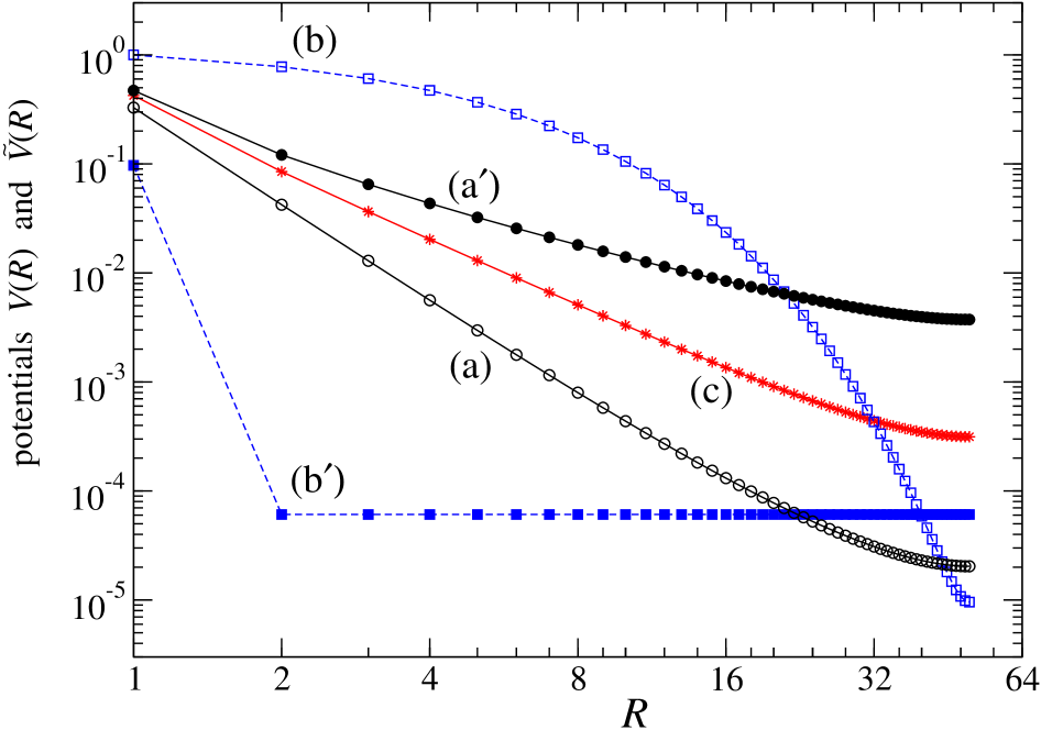
Figure 1: Three examples of a potential $V(R)$ and its dual $\widetilde{V}(R)$ on a ring of $N=100$ sites. (a) Open black circles: The power law potential $V(R)=\pi^{-1}N^{3}/[R(N-R)]^{3}$, appropriately symmetrized to satisfy equation (6); for $N\to\infty$ it tends to $V(R)=1/(\pi R^{3})$. (a^′): Its dual (filled black circles); for $N\to\infty$ it tends to a potential that decays with distance as $\sim 1/R$. (b) Open blue squares: The exponential potential $V_{\rm exp}(R)$ of equation (22) for $\alpha=0.25$. (b^′): Its dual (filled blue squares), equations (23) and (24). (c) Red stars: The self-dual potential $V(R)=\widetilde{V}(R)=V^{\star}(R)$, equation (72).

For future use we introduce an auxiliary potential $U(R)$,

$$U(R)=-\frac{1}{{\cal N}}\sum_{K\neq 0}\frac{1-\cos(KR)}{\widehat{V}(0)-\widehat{V}(K)},\qquad R=0,1,2,\ldots,{\cal N},$$ (25)

in which $\widehat{V}(0)-\widehat{V}(K)>0$. It is easily checked that $\widetilde{V}(R)$ may be derived from $U(R)$ by

$$\widetilde{V}(R)=U(R+1)+U(R-1)-2U(R),\qquad R=1,2,\ldots,{\cal N}-1,$$ (26)

a relation that appears in reference [2] (but with another normalization). This $U(R)$ arises through the well-known correspondence between a DG model and a lattice model in which the Hamiltonian reads $\frac{1}{2}\sum_{i\in\mathbb{Z}_{\cal N}}\sum_{i^{\prime}\in\mathbb{Z}_{\cal N}}U(i-i^{\prime})q_{i}q_{i^{\prime}}$ and the configurations of integer $q_{i}$’s obey the neutrality constraint $\sum_{i}q_{i}=0$. Therefore the integer-valued $q_{i}$ are called “charges” and their interaction potential $U$ the “charge potential.” Consequently equation (26) shows that $\widetilde{V}(R)$ is the potential created by a quadrupole of charges $1$ ,$-2$, and $1$ located on the sites $R=-1$, $R=0$, and $R=1$, respectively. We shall therefore sometimes refer to $\widetilde{V}(R)$ as the “quadrupolar interaction.”

2.3 DG model on a torus

In the special case of an $N\times M$ lattice with toroidal boundary conditions we shall write the DG Hamiltonian (1) as ${{\cal H}}_{2}$. Sites will be labeled by $\mathbf{i}=(i,j)$, where $i=0,1,\ldots,N-1$ and $j=0,1,\ldots,M-1$. The Hamiltonian (1) then becomes

$${{\cal H}}_{2}=\frac{1}{2}\sum_{(i,j)\in\mathbb{Z}_{N}\times\mathbb{Z}_{M}}\sum_{(i^{\prime},j^{\prime})\in\mathbb{Z}_{N}\times\mathbb{Z}_{M}}v(i-i^{\prime},j-j^{\prime})(h_{i,j}-h_{i^{\prime},j^{\prime}})^{2}.$$ (27)

Parity symmetry is now expressed as

$$v(r,s)=v(-r,-s).$$ (28)

Since the labels $(i,j)$, $(i+N,j)$, and $(i,j+M)$ refer to the same site, the potential $v$ must have the periodicity properties

$$v(r+N,s)=v(r,s),\qquad v(r,s+M)=v(r,s).$$ (29)

As a consequence of (28) and (29) we have the reflection symmetry

$$v(N-r,M-s)=v(r,s).$$ (30)

For $M=1$ this system reduces to the ring model described above.

Again, the Hamiltonian (27) is independent of the value of the interaction constant $v(0,0)$. The partition function is defined as in (7),

$$Z_{N,M}[\beta v]=\sideset{}{{}^{\prime}}{\sum}_{\{h_{i,j}\,|(i,j)\neq(0,0)\}}\exp[{-\beta{{{\cal H}}}_{2}}],$$ (31)

where the prime denotes the gauge condition $h_{0,0}=0$.

We shall consider in this work only functions on the ring and on the torus that have the symmetry properties (4)-(6) and (28)-(30), respectively.

3 Mapping between a torus and a ring

In this section we show how, under the condition that $N$ and $M$ are coprime, the Chinese remainder theorem allows us to introduce a mapping between the ring $\mathbb{Z}_{NM}$ and the torus $\mathbb{Z}_{N}\times\mathbb{Z}_{M}$ for both coordinates and periodic functions. For the Chinese remainder theorem at an elementary level see reference [5] and for more advanced topics see reference [6].

3.1 Mapping for spatial coordinates

3.1.1 Chinese remainder theorem

For any bijection of the sites $(r,s)$ of the torus $\mathbb{Z}_{N}\times\mathbb{Z}_{M}$ onto the integers $R$ of the ring $\mathbb{Z}_{NM}$ the Hamiltonian (27) becomes formally a one-dimensional Hamiltonian. We wish, however, to apply a bijection that preserves the group law (i.e., translation and inversion). The Chinese remainder theorem provides such a bijection at the condition that $N$ and $M$ be coprime, that is, that their only positive common divisor be unity. We shall henceforth take $M$ and $N$ such that this condition is met.

In the case of two integers $N,M>1$ the Chinese remainder theorem may be stated as follows. For any given pair of integers $(r,s)$ the set of equations with unknown $R$,

$$r=R\pmod{N},\qquad s=R\pmod{M},$$ (32)

where $x=y\pmod{N}$ means that $x$ and $y$ differ by a multiple of $N$, has a solution given by

$$R=aNs+bMr\pmod{NM},$$ (33a)

in which the pair of integer Bézout coefficients  $$(a,b)$$ is, in turn, a solution of

$$aN+bM=1.$$ (33b)

Bézout’s theorem guarantees that there exists a pair $(a,b)$ satisfying (33b) which may be found by the so-called extended Euclidean algorithm. The linear combination in (33a) is readily shown to satisfy the set of equations (32) as follows. By construction $aNs+bMr=bMr\pmod{N}$; then according to the identity (33b), $bMr$ can be rewritten as $r-aNr$ and $r-aNr=r\pmod{N}$. As a result $aNs+bMr=r\pmod{N}$. A similar argument leads to $aNs+bMr=s\pmod{M}$.

We notice that from the definition (33b) of the Bézout coefficients it immediately follows that another pair of the form $(a+cM,b-cN)$, where $c$ is any integer, is also a solution. We may make the solution of (33b) unique by imposing, for example, that $0<a<M$ and $-N<b<0$, or, alternatively, that $-M<{a}<0$ and $0<{b}<N$. With the constraint $0<a<M$ and $-N<b<0$, we give the solutions for various special cases of $N$ and $M$. For $N>1$ and $M=2$, the solution is $a=1$ and $b=(1-N)/2$; for $N>2$ and $M=N-1$ one gets $a=1$ and $b=-1$; and for $M>1$ and $N=qM+1$, where $q=2,3,\ldots$, one finds $a=1$ and $b=-q$.

3.1.2 Geometrical interpretation

The Chinese remainder theorem may be interpreted as a helicoidal mapping of a one-dimensional path around the $N\times M$ torus in the following way. We refer to figure 2. We let $R$ take the successive values $R=0,1,2,\ldots,NM$ and consider the path traced out on the torus by the pair $(r,s)$ parametrized by $R$ according to equation (32). At $R=0$ the path starts in the origin $(r,s)=(0,0)$, and as long as $R<\min(N,M)$ we have $(r,s)=(R,R)$, that is, the path follows the main diagonal, undergoing at each step an increment $(1,1)$. For larger $R$ the path continues to undergo increments $(1,1)$, but the $N,M$-periodicity of the lattice has to be taken into account. This leads to a path that winds around the torus until it returns to the origin. The condition that $N$ and $M$ be coprime guarantees that this return will occur only after the path has visited all sites of the torus.

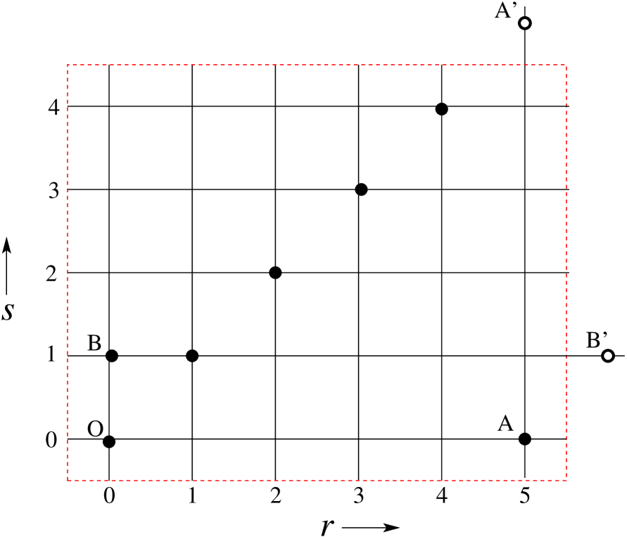
Figure 2: The sites of an $N\times M$ toroidal lattice with $N=6$ and $M=5$. The fundamental domain is the region inside the dashed red rectangle, which must be considered as periodically repeated; in particular, $A$ and $A^{\prime}$ are identical sites, and so are $B$ and $B^{\prime}$. The path described in the text starts at the origin $O$ and moves at each step diagonally in the direction $(1,1)$, as indicated by the black dots. When it steps to site $A^{\prime}$, it leaves the fundamental domain but in fact arrives at $A$. Its subsequent step in the $(1,1)$ direction then takes it to $B^{\prime}$, but in fact it arrives at $B$. Upon continuing it will visit all lattice sites until at its $NM$th step it returns to $O$.

3.1.3 Another mapping and corresponding helicoidal winding

In section (3.2) we shall show that the functions $F(R)\equiv f(r,s)$ defined with the mapping (33a) are periodic with period $MN$. We notice that we could have chosen another helix which winds around the torus while also preserving the periodicity of the lattice, so that the corresponding mapping $(r,s)\mapsto R^{\prime}$ leads to the same periodicity $NM$ for functions $F^{\prime}(R^{\prime})\equiv f(r,s)$.

For instance another proper helix is built by again mapping the origin $(r,s)=(0,0)$ onto the integer $R=0$ and then by incrementing the position on the $N\times M$ lattice by steps of $(-1,1)$ while at the same time increasing $R$ by one unit. After $R^{\prime}$ steps on the helix the corresponding coordinates on the torus are

$$r=-R^{\prime}\pmod{N},\qquad s=R^{\prime}\pmod{M}.$$ (34)

A simple argument similar to that presented for the derivation of the Chinese theorem (33) shows that the linear combination

$$R^{\prime}=aNs-bMr$$ (35)

is a solution of (34), because $a$ and $b$ are the solutions of (33b). We shall see in subsection (4.3) how the results of interest in the present paper depend on the choice of one among the two mappings $R=aNs+bMr$ or $R^{\prime}=aNs-bMr$.

3.2 Mapping for periodic functions

3.2.1 Periodicity on the torus and on the ring

Let $f(r,s)$ be a given biperiodic function on the $N\times M$ torus obeying the symmetry properties (28)-(30).

$$f(r+N,s)=f(r,s+M)=f(r,s)$$ (36)

and

$$f(N-r,M-s)=f(r,s).$$ (37)

We define a corresponding function $F(R)$ on the ring of length $NM$ by

$$F(R)=f(r,s)\quad\textrm{with}\quad R=aNs+bMr\pmod{NM}.$$ (38)

We shall show that the symmetries of $f$ imply those of $F$ and that the reciprocal is also true.

The pairs $(r+N,s)$ and $(r,s+M)$ are associated with $R+bNM$ and $R+aNM$, respectively. The periodicity properties (36) then lead to $F(R+bMN)=F(R+aMN)=F(R).$ It follows that $F(R)=\break F(R+N(aNM)+M(bNM))$, whence, with the use of (33b), we find that

$$F(R+NM)=F(R).$$ (39)

Similarly, by virtue of (33b), the reflected point $(N-r,M-s)$ is associated with $aN(M-s)+bM(N-r)=NM-R$, and the symmetry property (37) leads to

$$F(NM-R)=F(R).$$ (40)

As a consequence we also have the third symmetry, $F(-R)=F(R)$; that is, $F$ obeys the symmetries (28)-(30) for a ring of $NM$ sites. We point out that similar arguments show that the periodicity (39) and the reflection symmetry (40) are also valid for the second mapping (35).

Let conversely $F(R)$ be given and satisfy (39) and (40); then $f(r+N,s)=f(r,s+M)=f(r,s)$ and $f(N-r,M-s)=f(r,s)$ . Indeed if $F(R+NM)=F(R)$ then $F(R+aNM)=F(R)$, and $R+aNM$ corresponds to $(r,s+M)$. Similarly if $F(NM-R)=F(R)$ then $F((a+b)NM-R)=F(R)$, and $(a+b)NM-R$ corresponds to $(N-r,M-s)$.

3.2.2 Mapping Fourier transforms from the torus to the ring

The Fourier transform of an $NM$-periodic function $F(R)$ on the ring of length $NM$ is

$$\widehat{F}(K)=\sum_{R\in\mathbb{Z}_{NM}}\mbox{e}^{-{\rm i}KR}\,F(R)$$ (41)

with the wavenumbers

$$K=\frac{2\pi}{NM}p,$$ (42)

where $p\in\mathbb{Z}_{NM}$. Similarly, the Fourier transform of an $N,M$-biperiodic function $f(r,s)$ on the torus is

$$\widehat{f}(k_{1},k_{2})=\sum_{r\in\mathbb{Z}_{N}}\sum_{s\in\mathbb{Z}_{M}}\mbox{e}^{-{\rm i}(k_{1}r+k_{2}s)}\,f(r,s)$$ (43)

with the wavenumbers

$$k_{1}=\frac{2\pi}{N}n,\qquad k_{2}=\frac{2\pi}{M}m,$$ (44)

where $n\in\mathbb{Z}_{N}$ and $m\in\mathbb{Z}_{M}$. We now investigate the relation that results between these two Fourier transforms in case $F(R)=f(r,s)$.

The Chinese remainder theorem allows us to establish a bijection between the index $p$ of the wavenumber on the ring and the index pair $(n,m)$ on the torus,

$$p=aNm+bMn\pmod{NM},$$ (45)

which is analogous to $R=aNs+bMr\pmod{NM}$. Hence the wavenumber on the torus may be expressed in terms of those on the ring as

$$K=bk_{1}+ak_{2}.$$ (46)

After some rewriting and use of identity (33b) we find

$$\mbox{e}^{-{\rm i}KR}=\mbox{e}^{-{\rm i}(bk_{1}r+ak_{2}s)}.$$ (47)

When we substitute (46) in (41) and identify $F(R)=f(r,s)$, we obtain

$$\widehat{F}(K)=\sum_{r\in\mathbb{Z}_{N}}\sum_{s\in\mathbb{Z}_{M}}\mbox{e}^{-{\rm i}(bk_{1}r+ak_{2}s)}f(r,s)=\widehat{f}(bk_{1},ak_{2}).$$ (48)

The Fourier transform $\widehat{F}(K)$ on the ring proves to coincide with a scaled Fourier transform on the torus. Relation (48) allows to determine the Fourier transform $\widehat{F}(K)$ on the ring when the Fourier transform $\widehat{f}(k_{1},k_{2})$ on the torus is given.

3.2.3 Mapping Fourier transforms from the ring to the torus

We shall now see how to determine the Fourier transform $\widehat{f}(k_{1},k_{2})$ on the torus when the Fourier transform $\widehat{F}(K)$ on the ring is given. We first write $f(r,s)=F(R)=\frac{1}{MN}\sum_{K}\mbox{e}^{{\rm i}KR}\widehat{F}(K)$, and from (46) and (47) we get

$$f(r,s)=\frac{1}{MN}\sum_{(k_{1},k_{2})}\mbox{e}^{{\rm i}(bk_{1}r+ak_{2}s)}\widehat{F}(bk_{1}+ak_{2}).$$ (49)

where $(k_{1},k_{2})$ is related to a pair of integers $(n,m)$ through (44).

We then notice that, according to (33b), the coefficient $b$ is coprime with $N$ (because if $b$ and $N$ had a common divisor different from $1$ or $-1$ then $aN+bM$ could not be equal to $1$). By virtue of Gauss’s lemma, the fact that there exists no common divisor of $b$ and $N$ entails that if $b(n-n^{\prime})$ is a multiple of $N$, then $n-n^{\prime}$ is also a multiple of $N$. Equivalently $n\neq n^{\prime}\pmod{N}$ implies $bn\neq bn^{\prime}\pmod{N}$ and $n\mapsto bn$ is a one-to-one correspondence from $\mathbb{Z}_{N}$ to $\mathbb{Z}_{N}$. Similarly, according to (33b), the coefficient $a$ is coprime with $M$ and $m\mapsto am$ is a one-to-one correspondence from $\mathbb{Z}_{M}$ to $\mathbb{Z}_{M}$. As a result, if the function $A(n,m)$ is $N,M$-periodic, then

$$\sum_{(n,m)\in\mathbb{Z}_{N}\times\mathbb{Z}_{M}}A(bn,am)=\sum_{(n,m)\in\mathbb{Z}_{N}\times\mathbb{Z}_{M}}A(n,m).$$ (50)

Hence the sum in (49) can be rewritten without the coefficients $a$ and $b$, and eventually

$$f(r,s)=\frac{1}{MN}\sum_{(k_{1},k_{2})}\mbox{e}^{{\rm i}(k_{1}r+k_{2}s)}\widehat{F}(k_{1}+k_{2}).$$ (51)

Upon Fourier transforming both members of this equation we find

$$\widehat{f}(k_{1},k_{2})=\widehat{F}(k_{1}+k_{2}),$$ (52)

which is the desired relation that yields $\widehat{f}(k_{1},k_{2})$ when $\widehat{F}(K)$ is given.

4 New duality for two-dimensional DG models

4.1 Mapping between torus and ring Hamiltonians

In the preceding section we have defined a mapping between the sites of the torus and those of the ring, and an identification of functions defined on the torus with functions defined on the ring. Now we consider how a Hamiltonian given on the torus transforms into one defined on the ring.

Let the Hamiltonian ${{\cal H}}_{2}$ of equation (27) be given. A mapping of this Hamiltonian, defined on the torus $\mathbb{Z}_{N}\times\mathbb{Z}_{M}$, onto a Hamiltonian on the ring $\mathbb{Z}_{NM}$ is constructed as follows. We relabel the height variables $h_{r,s}$ according to

$$h_{R}=h_{r,s}\,,$$ (53)

where $R$ is given by (33) and we define the potential $V(R)$ by

$$V(R)=v(r,s).$$ (54)

According to section (3.2) the periodicity properties (29) and the reflection symmetry (30) of $v(r,s)$ imply that

$$V(R)=V(R+MN)$$ (55)

and

$$V(R)=V(MN-R).$$ (56)

When we express the two-dimensional DG Hamiltonian ${{\cal H}}_{2}$ defined in (27) in terms of the new quantities $V(R)$ and $h_{R}$, we find that ${{\cal H}}_{2}$ becomes a one-dimensional DG Hamiltonian of type (3),

$${{\cal H}}_{1}[V]=\frac{1}{2}\sum_{i\in\mathbb{Z}_{MN}}\sum_{R\in\mathbb{Z}_{MN}}V(R)(h_{i}-h_{i+R})^{2},$$ (57)

and the partition functions of the two models are identical,

$$Z_{N,M}\left[\beta v\right]=Z_{NM}\left[\beta V\right].$$ (58)

Hence we have identified the partition function on the torus with a partition function on the ring.

4.2 Duality on the torus

Relation (58) embodies the mapping of a given two-dimensional system with potential $v$ onto a one-dimensional one with related potential $V$. We may now apply, without recalling all the intermediary steps, the mechanism of section 2.2 whereby $V(R)$ is related to a dual one-dimensional potential $\widetilde{V}(R)$. Subsequently we return to a dual two-dimensional potential $\widetilde{v}(r,s)$ by means of the relation

$$\widetilde{v}(r,s)=\widetilde{V}(R),$$ (59)

Because of (21) the dual potential also has the reflection property on the torus

$$\widetilde{v}(r,s)=\widetilde{v}(N-r,M-s).$$ (60)

The corresponding DG partition function is given by the identity (58),

$$Z_{N,M}\left[\beta\,\widetilde{v}\right]=Z_{NM}\left[\beta\,\widetilde{V}\right].$$ (61)

By combining the duality relation (15) between the partition functions on the ring with (58) and (61) we obtain the two-dimensional duality

$$Z_{N,M}\left[\beta\,v\right]=\frac{1}{\beta^{(MN-1)/2}}C_{NM}[V]\,\,Z_{N,M}\left[\frac{\pi^{2}}{\beta}\,\widetilde{v}\right].$$ (62)

In the relation (62) the constant $C_{NM}[V]$, given in (16), is still a functional of the intermediate one-dimensional potential $V$. We re-express it as follows as a functional $c_{N,M}[v]$ of $v$. Indeed, $W(K)=\widehat{V}(0)-\widehat{V}(K)$ and, according to (48) a Fourier transform on the ring is equal to a scaled Fourier transform on the torus. Hence we have

$$C_{NM}[V] = \sqrt{NM}\left[\prod_{(n,m)\in\mathbb{Z}_{N}\times\mathbb{Z}_{M}\backslash(0,0)}\frac{\pi}{\widehat{v}(0,0)-\widehat{v}(2\pi bn/N,2\pi am/M)}\right]^{1/2}$$ (63)

$$= \sqrt{NM}\left[\prod_{(k_{1},k_{2})\neq(0,0)}\frac{\pi}{\widehat{v}(0,0)-\widehat{v}(k_{1},k_{2})}\right]^{1/2}$$

$$\equiv c_{N,M}[v]$$

where to arrive at the second line we have used the property (50), and we used the notation $k_{1}=2\pi n/N$ and $k_{2}=2\pi m/M$. Eventually the duality relation (62) between partition functions on the torus reads in terms of functions defined on the torus

$$Z_{N,M}\left[\beta v\right]=\frac{1}{\beta^{(NM-1)/2}}c_{N,M}[v]\,\,Z_{N,M}\left[\frac{\pi^{2}}{\beta}\widetilde{v}\right].$$ (64)

This achieves the purpose of establishing a duality relation for partition functions on the torus.

The relation between the given potential $v(r,s)$ and its dual $\widetilde{v}(r,s)$ may be rendered more explicit. As in the one-dimensional case, $\widetilde{v}(r,s)$ may be re-expressed in terms of the Fourier transform of $v(r,s)$ as follows. According to (52) the Fourier transform on the torus for $\widetilde{v}(r,s)$ is given in terms of the Fourier transform on the ring for $\widetilde{V}(R)$ by $\widehat{\widetilde{v}}(k_{1},k_{2})=\widehat{\widetilde{V}}(k_{1}+k_{2})$, while the expression for $\widetilde{V}(K)$ in terms of $V(K)$ is given by (18). As a result $\widehat{\widetilde{v}}(k_{1},k_{2})-\widehat{\widetilde{v}}(0,0)=2[1-\cos(k_{1}+k_{2})]/[\widehat{V}(k_{1}+k_{2})-\widehat{V}(0)]$. By using again relation (52) to go back from the ring to the torus, namely $\widehat{V}(k_{1}+k_{2})=\widehat{v}(k_{1},k_{2})$, we find that the Fourier transform of the dual potential on the torus takes the simple form

$$\widehat{\widetilde{v}}(k_{1},k_{2})-\widehat{\widetilde{v}}(0,0)=-\frac{2[1-\cos(k_{1}+k_{2})]}{\widehat{v}(0,0)-\widehat{v}(k_{1},k_{2})}.$$ (65)

Subsequently the expression of the dual potential $\widetilde{v}(r,s)$ in terms of $v(r,s)$ is given by the inverse Fourier transform on the torus, for $(r,s)\neq(0,0)$

$$\widetilde{v}(r,s)=\ -\frac{1}{MN}\sum_{(k_{1},k_{2})\neq(0,0)}\mbox{e}^{{\rm i}[k_{1}r+k_{2}s]}\frac{2[1-\cos(k_{1}+k_{2})]}{\widehat{v}(0,0)-\widehat{v}(k_{1},k_{2})}$$ (66)

with $\widehat{v}(0,0)-\widehat{v}(k_{1},k_{2})>0$ for $(k_{1},k_{2})\neq(0,0)$. An explicit example of the duality embodied by equation (65) will be considered in section 6.

Finally, we may check that the square of the duality transformation is the identity. Indeed, iteration of the duality relation (64) leads to $Z_{N,M}\left[\beta v\right]=(1/\pi)^{NM-1}\,c_{N,M}[v]c_{N,M}[\widetilde{v}]\,Z_{N,M}\left[\beta\widetilde{\widetilde{v}}\right]$, where $\widetilde{\widetilde{v}}=v$ according to (65), while the identity $\prod_{K\neq 0}2|\sin(K/2)|=NM$ implies that $c_{N,M}[v]c_{N,M}[\widetilde{v}]$ $=c_{N,M}[V]c_{N,M}[\widetilde{V}]$ $=\pi^{NM-1}$.

We notice that for a given mapping the expressions for the constant $c_{N,M}$ and the dual potential are independent of the Bézout coefficients $(a,b)$ according to (63) and (66). As a result we could have chosen the pair of Bézout coefficients $(\overline{a},\overline{b})$ such that $-M<\overline{a}<0$ and $0<\overline{b}<N$ with the mapping $\overline{R}=\overline{a}Ns+\overline{b}Mr\pmod{NM}$ without changing the duality relation between the partition functions nor the expression of the dual potential $\widetilde{v}$ in terms of the potential $v$.

4.3 Dependence of the dual potential upon the choice of the mapping

As noticed above, the constant $c_{N,M}$ as well as the relation between the Fourier transforms of the dual potentials on the torus prove to be independent of $a$ and $b$ for a given mapping. However the dependence upon the choice of the mapping can be exemplified by the comparison of the two mappings presented in section (3.1.2) and (3.1.3).

With the mapping $R=aNs+bMr$, the coordinates $R$ and $R\pm 1$ correspond to $(r,s)$ and $(r\pm 1,s\pm 1)$, respectively. Then the relation (26) between $\widetilde{V}(R)$ and $U(R)$ implies that $\widetilde{v}(r,s)=V(aNs+bMr)$ may be rewritten as

$$\widetilde{v}(r,s)=u(r+1,s+1)+u(r-1,s-1)-2u(r,s),$$ (67)

where, by using (25),

$$u(r,s)=\frac{1}{MN}\sum_{(k_{1},k_{2})\neq(0,0)}\left[\cos(k_{1}r+k_{2}s)-1\right]\frac{1}{\widehat{v}(0,0)-\widehat{v}(k_{1},k_{2})}.$$ (68)

(The latter relation may also be directly derived from the inverse Fourier transform representation (66) for $\widetilde{v}(r,s)$, as was done to derive (26)-(25) from (19).) With the other mapping the coordinates $R^{\prime}=aNs-bMr$ and $R^{\prime}\pm 1$ correspond to $(r,s)$ and $(r\mp 1,s\pm 1$), respectively. Then relation (26) on the ring implies that $\widetilde{v}^{\prime}(r,s)=V(aNs-bMr)$ and may be rewritten as

$$\widetilde{v}^{\prime}(r,s)=u(r+1,s-1)+u(r-1,s+1)-2u(r,s),$$ (69)

with the same potential $u(r,s)$ as in relation (67) for the first mapping.

With the terminology introduced after (26), in the case of the first mapping $\widetilde{v}(r,s)$ appears as a quadrupolar charge interaction, with charges $(1,-2,1)$ aligned at points $(-1,-1)$, $(0,0)$, and $(1,1)$, respectively, along the direction of the first mapping helix. For the second mapping $\widetilde{v}^{\prime}(r,s)$ still appears as a quadrupolar charge interaction with the same charge triplet, but the charges are located at different points, namely $(-1,1)$, $(0,0)$, and $(1,-1)$, respectively, along the direction of the second mapping helix at a given point.

The interaction $u$ is definitely independent of the mapping by virtue of (68). However the above discussion shows that the dual potential $\widetilde{v}$ depends on the mapping since it is a quadrupolar interaction (involving the charge-charge interaction $u$) and the locations of the charges in the quadrupole depend on the mapping.

This investigation ultimately proves that the different options presented in section 3 for the choice of the path in figure 1 amount to carrying out reflection symmetries with respect to the $r$ and/or $s$ axes. They do not result in any essentially new dualities.

5 Self-duality

5.1 Self-dual potential and self-dual temperature

As shown in reference [2], the relation between the potentials $V(R)$ and $\widetilde{V}(R)$ on the ring, which is given by relation (18) between their Fourier transforms, leads to the existence of a self-dual potential  $V^{\star}(R)$ such that for any $R\neq 0$

$$\widetilde{V^{\star}}(R)=V^{\star}(R).$$ (70)

Indeed, according to (18), if for $K\neq 0$

$$\widehat{V^{\star}}(K)-\widehat{V^{\star}}(0)=-2|\sin(K/2)|,$$ (71)

then $\widehat{\widetilde{V^{\star}}}(K)-\widehat{\widetilde{V^{\star}}}(0)=\widehat{V^{\star}}(K)-\widehat{V^{\star}}(0)$, namely $\widetilde{W^{\star}}(K)=W^{\star}(K)=2|\sin(K/2)|$. The expression for $V^{\star}(R)$ when $R\neq 0$ is obtained by inserting (71) in (13). The potential $V^{\star}(R)$ is periodic in $R$ with period $MN$ and it may be written in various forms. For the following discussion we write

$$V^{\star}(R)=\frac{\frac{1}{MN}\sin\frac{\pi}{MN}}{\sin^{2}(\frac{\pi}{MN}R)-\sin^{2}(\frac{\pi}{2MN})}.$$ (72)

For the corresponding self-dual potential on the torus, $v^{\star}(r,s)=V^{\star}(R)$ with $R=aNs+bMr$. Moreover $c_{N,M}[v^{\star}]=C_{NM}[V^{\star}]=\pi^{(NM-1)/2}$ according to definition (16) and the identity $\prod_{K\neq 0}2|\sin(K/2)|=NM$. Therefore when $v=v^{\star}$ the duality relation (64) for partition functions becomes

$$Z_{N,M}\left[\beta v^{\star}\right]=\left(\frac{\beta^{\star}}{\beta}\right)^{(NM-1)/2}\,\,Z_{N,M}\left[\frac{{\beta^{\star}}^{2}}{\beta}v^{\star}\right]$$ (73)

with $\beta^{\star}=\pi$. This equation shows that there is a self-dual (inverse) temperature  $\beta=\beta^{\star}=\pi$ at which (73) becomes a trivial identity. In the next two sections we shall first investigate the self-dual potential $v^{\star}$ and then the height-height correlation function for this potential when the system is at the dual temperature $\beta=\beta^{\star}$.

5.2 Self-dual potential for large $N$

We now investigate some of the properties of this two-dimensional self-dual potential. We wish to consider its limit for a strip of infinite length and finite width, $N\to\infty$ with $M$ fixed, and for an infinite lattice, $N\to\infty$ and $M\to\infty$. By virtue of (72) the explicit expression of $v^{\star}(r,s)=V^{\star}(R)$ is in fact a function of $R/(NM)$. In order to study the large-$N$ limit of $v^{\star}(r,s)$ it is convenient to make the change of variables $(r,s)\mapsto(r,t)$ with

$$t=s-r,$$ (74)

which, with the use of the identities (33), leads to rewriting $R$ as $R=aNt+r$. Then $R/(NM)$ becomes

$$\frac{R}{MN}=\frac{at}{M}+\frac{r}{MN},$$ (75)

and, according to (72), the self-dual potential $v^{\star}(r,s)$ becomes the function

$$v^{\star}(r,r+t)=\frac{\frac{1}{MN}\sin\frac{\pi}{MN}}{\sin^{2}\pi\big{(}\frac{at}{M}+\frac{r}{MN}\big{)}-\sin^{2}\big{(}\frac{\pi}{2MN}\big{)}}.$$ (76)

For coordinate differences $(r,r)$ we have that $t=0$ and

$$v^{\star}(r,r)=\frac{\frac{1}{MN}\frac{\pi}{MN}}{\sin^{2}\pi\big{(}\frac{r}{MN}\big{)}-\sin^{2}\big{(}\frac{\pi}{2MN}\big{)}},$$ (77)

which depends only on $MN$. Therefore when $N$ goes to infinity, and whether or not $M$ remains finite, equation (77) gives

$$\lim_{N\to\infty}v^{\star}(r,r)=\frac{1}{\pi\left[r^{2}-\tfrac{1}{4}\right]}\,.$$ (78)

For coordinate differences $(r,s)$ with $s\neq r$ we have to distinguish between $M$ remaining finite or tending to infinity, and we must know the Bézout coefficient $a$ as a function of $N$ and $M$. We shall choose to take

$$N=qM+1,$$ (79)

with $q$ an arbitrary positive integer, which ensures that $N$ and $M$ are coprime. In this case $a=1$ and $b=-q$. Then, by virtue of (76), $v^{\star}(r,r+t)$ becomes a function of $\frac{t}{M}+\frac{r}{MN}$.

In order to study strips of finite width $M$ we consider the scaling (79) with $M$ fixed and $q\to\infty$, whence $N\to\infty$. For $M=2$ the torus is the ladder lattice with each interchain bond counting twice, and for $M=4$ it is a beam with a square section. Then for $r$ and $t\neq 0$ fixed, $t/M$ remains finite while $r/(MN)$ vanishes. Upon inserting this limit behavior in equation (76) and restoring the original coordinates $r$ and $s$ we find

$$v^{\star}(r,s)\simeq\frac{\pi}{M^{2}N^{2}\sin^{2}\pi\big{(}\frac{r-s}{M}\big{)}}\,,\qquad N\to\infty,\,\,M\mbox{ fixed}.$$ (80)

A two-dimensional infinite lattice is obtained when both $M$ and $N$ go to infinity with $q$ fixed. For $r$ and $t$ fixed, $r/MN$ and $1/(2MN)$ vanish faster than $t/M$, and expression (76) tends to the limit

$$v^{\star}(r,s)\simeq\frac{1}{N^{2}\pi(r-s)^{2}}.$$ (81)

In all cases considered above

$$\lim_{N\to\infty}v^{\star}(r,s)=\frac{\delta_{r,s}}{\pi\left[r^{2}-\tfrac{1}{4}\right]}\,.$$ (82)

This says that in the limit $N\to\infty$ each height variable on a given site $(i,j)$ interacts only with the height variables on the diagonal $(i+r,j+r)$ passing through that site in the direction $(1,1)$, and we recover the large distance behavior of the potential (72) on the one-dimensional chain of length $MN$ in the limit $MN\to\infty$.

5.3 Self-dual height-height correlation at $\beta^{\star}$

Let $h_{\mathbf{i}+\mathbf{r}}-h_{\mathbf{i}}$ be the difference between two height variables at sites $\mathbf{i}$ and $\mathbf{i}+\mathbf{r}$ in either dimension $1$ or $2$. By symmetry we have that $\langle h_{\mathbf{i}+\mathbf{r}}-h_{\mathbf{i}}\rangle_{\beta}=0$. However the correlation

$$g(\mathbf{r};\beta)\equiv\langle(h_{\mathbf{i}+\mathbf{r}}-h_{\mathbf{i}})^{2}\rangle_{\beta}$$ (83)

is a nonvanishing and interesting function of $\mathbf{r}$.

For the DG model on a ring it was shown in reference [2] that, although the correlation $G(R;\beta)\equiv\langle(h_{i+R}-h_{i})^{2}\rangle_{\beta}$ is not known for a generic potential $V(R)$ at any inverse temperature $\beta$, the duality relation (15) for the partition functions implies that this correlation can be explicitly determined in the case of the self-dual potential $V^{\star}(R)$ at the dual temperature $\beta^{\star}=\pi$ defined after (73). It reads

$$G^{\star}(R;\beta^{\star})=-\frac{1}{2\pi}U^{\star}(R),$$ (84)

where the superscript $\star$ of the correlation $G$ signals a statistical average with the potential $V^{\star}(R)$ and where $U^{\star}(R)$ is the periodic potential associated with $V^{\star}(R)$ by (26) and which vanishes at $R=0$. Relation (26) can be seen as a finite difference equation to be solved for $R$ in the set $\{0,1,\ldots,MN\}$ with the boundary conditions $U^{\star}(0)=U^{\star}(NM)=0$. By rewriting expression (72) for $V^{\star}(R)$ as a difference of cotangents with arguments proportional to $R+1$ and $R$ we find that for $R=0,1,\ldots,NM$

$$U^{\star}(R)=-\frac{1}{NM}\sum_{R^{\prime}=1}^{R}\cot\frac{\pi}{NM}\left(R^{\prime}-\frac{1}{2}\right),$$ (85)

with the understanding that for $R=0$ the sum is empty. The expression for $U^{\star}(R)$ when $R=-NM,-NM+1,\ldots,-1,0$ is obtained by using the periodicity property $U^{\star}(-|R|)=U^{\star}(NM-|R|)$ derived from (25) and rewriting the sum for $U^{\star}(NM-|R|)$ by taking into account the value $U^{\star}(NM)=0$. The result is that for $R=-NM,-NM+1,\ldots,NM$ we have

$$U^{\star}(R)=-\frac{1}{NM}\sum_{R^{\prime}=1}^{|R|}\cot\frac{\pi}{NM}\left(R^{\prime}-\frac{1}{2}\right).$$ (86)

For the DG model on a torus an argument similar to that presented in reference [2] shows that, for the potential $v^{\star}(r,s)=V^{\star}(R)$ at the inverse dual temperature $\beta^{\star}$, the correlation $g^{\star}(r,s;\beta^{\star})=\langle(h_{i+r,j+s}-h_{i,j})^{2}\rangle^{\star}_{\beta^{\star}}$ can be determined as

$$g^{\star}(r,s;\beta^{\star})=-\frac{1}{2\pi}u^{\star}(r,s)$$ (87)

in which

$$u^{\star}(r,s)=U^{\star}(R).$$ (88)

Since for the model on the ring $U^{\star}(R)$ is known, equations (87) and (88) allow us to determine the explicit expression for $g^{\star}(r,s;\beta^{\star})$ on the torus. This will be the subject of the next subsection.

5.4 Height-height correlation in the thermodynamic limit for $N=M+1$

In the present section we consider the thermodynamic limit where $N=M+1$ and $N$ goes to infinity. Then $M$ and $N$ are coprime, $a=1$, and $R=r+N(s-r)$. Before taking the limit we consider the variables $r$ and $s$ in intervals centered at $(0,0)$. If, for instance, $M$ is even, the intervals read

$$-\frac{M}{2}\leq r\leq\frac{M}{2}\qquad\textrm{and}\qquad-\frac{M}{2}<s\leq\frac{M}{2}.$$ (89)

5.4.1 Fixed coordinate differences

In the case of $r=s$ fixed we have that $u^{\star}(r,r)=U^{\star}(r)$ where $U^{\star}(r)$ is the sum up to $|r|$ given in (86). In the thermodynamic limit the argument of every cotangent in this sum is at least of order ${\cal O}(1/N^{2})$ so that we can replace $\cot x$ by $1/x$ and $u^{\star}(r,r)$ becomes

$$u^{\star}(r,r)=-\frac{1}{\pi}\sum_{r^{\prime}=1}^{|r|}\frac{1}{r^{\prime}-\frac{1}{2}}+{\cal O}\left(\frac{1}{N^{4}}\right).$$ (90)

Therefore when $r=s$ the correlation given by (87) is a nonvanishing function in the thermodynamic limit. It is denoted as $g^{\star}_{\infty}(r,r;\beta^{\star})$ and reads

$$g^{\star}_{\infty}(r,r;\beta^{\star})=\frac{1}{2\pi^{2}}\sum_{r^{\prime}=1}^{|r|}\frac{1}{r^{\prime}-\frac{1}{2}}.$$ (91)

For large $r$ it behaves as

$$g^{\star}_{\infty}(r,r;\beta^{\star})=\frac{1}{2\pi^{2}}\left[\ln|r|+A_{0}+{\cal O}\left(\frac{1}{r^{2}}\right)\right]$$ (92)

with $A_{0}=C+2\ln 2$ where $C$ denotes Euler’s constant.

In the case $r\neq s$ it is more convenient to make the change of variables $(r,s)\mapsto(r,t)$ with $s=r+t$ and to consider

$$g^{\star}(r,r+t;\beta^{\star})=-\frac{1}{2\pi}U^{\star}(Nt+r).$$ (93)

The expression for $U^{\star}(Nt+r)$ is the sum given in (86) with $M=N-1$ and $|t|<N$ according to (89). When $r$ and $s$ are kept fixed while $N$ and $M=N-1$ become very large, $t$ is fixed and $|r+Nt|\simeq N|t|$ with $N\leq N|t|\ll N^{2}$. Therefore the argument of every cotangent in the sum is at least of order ${\cal O}(1/N)$ and one can again replace $\cot x$ by $1/x$, while the upper bound of the sum is of order $N$. As a result in the thermodynamic limit the leading contribution in the correlation $g^{\star}(r,r+t;\beta^{\star})$ is the large distance behavior (92) of expression (91), where the argument $r$ is to be replaced by $Nt=N(s-r)$,

$$g^{\star}(r,s;\beta^{\star})\underset{r\neq s}{=}\frac{1}{2\pi^{2}}\left[\ln(N|s-r|)+A_{0}+o(1)\right],$$ (94)

in which $o(1)$ denotes a contribution that vanishes in the limit $N\to\infty$. Equation (94) expresses that when $N=M+1$, according to (81), two height variables on parallel diagonals have an interaction whose coupling constant decreases with $N$ so that the variance of their difference increases with $N$.

5.4.2 Coordinate differences scaled with the lattice size

Whereas in the preceding subsection we investigated the height-height correlation $g^{\star}(r,s;\beta^{\star})=-(1/2\pi)U^{\star}(R)$ in the regime of fixed $r$ and $s$ with $N=M+1$ and $N\to\infty$, it is also interesting to study the nature of this correlation at the scale of the system, that is, for fixed values of

$$\xi=\frac{r}{N},\qquad\eta=\frac{s}{N-1}$$ (95)

where, according to (89), $-\frac{1}{2}<\xi<\frac{1}{2}$, $-\frac{1}{2}<\eta\leq\frac{1}{2}$ and $N\to\infty$. Then

$$R=(\eta-\xi)N(N-1)\pmod{N(N-1)}$$ (96)

with $-1<\eta-\xi<1$. Equation (86) now leads to

$$U^{\star}\left((\eta-\xi)N(N-1)\right) = -\frac{1}{N(N-1)}\sum_{R^{\prime}=1}^{|\eta-\xi|N(N-1)}\cot\frac{\pi(R^{\prime}-\tfrac{1}{2})}{N(N-1)},$$ (97)

$$\equiv \overline{U^{\star}}(\eta-\xi).$$

with $\overline{U^{\star}}(0)=0$ according to (85). Since only the absolute value $|\eta-\xi|$ appears in the upper limit of the sum in (97), it suffices to calculate $\overline{U^{\star}}(\eta-\xi)$ with $0<\eta-\xi<1$. Moreover, according to expression (25) for $U^{\star}(R)$ as an inverse Fourier transform, and as can be checked on its explicit $R$-dependence given in (86), $U^{\star}(R)$ has the symmetry $U^{\star}(N(N-1)-R)=U^{\star}(R)$. Therefore $\overline{U^{\star}}(\eta-\xi)$ takes the same value for $\eta-\xi$ and $1-(\eta-\xi)$ and we may further restrict ourselves to $0<\eta-\xi<1/2$, which we shall do now.

With the present scaling, when $0<\eta-\xi<1/2$, the argument $\pi(R^{\prime}-\tfrac{1}{2})/(N(N-1))$ of the cotangent increment in the sum runs up to values of order $\pi/2$ and for every $R^{\prime}$ all terms in the large-$N(N-1)$ expansion of the cotangent contribute. Therefore we shall write $U^{\star}=I_{0}+I_{1}$, where $I_{0}$ and $I_{1}$ are the sums of the contributions of the first term and of all remaining terms, respectively, in the full expansion. This gives

$$I_{0} = -\frac{1}{\pi}\sum_{R^{\prime}=1}^{(\eta-\xi)N(N-1)}\frac{1}{R^{\prime}-\tfrac{1}{2}}$$ (98)

$$= -\frac{1}{\pi}\left[\ln\Big{(}(\eta-\xi)N(N-1)\Big{)}+A_{0}\right]+{\cal O}\left(\frac{1}{N^{4}}\right),$$

where we have used (92), and

$$I_{1} = -\frac{1}{N(N-1)}\sum_{R^{\prime}=1}^{(\eta-\xi)N(N-1)}\Big{[}\cot\frac{\pi(R^{\prime}-\tfrac{1}{2})}{N(N-1)}-\frac{N(N-1)}{\pi(R^{\prime}-\tfrac{1}{2})}\Big{]}$$ (99)

$$= -\frac{1}{\pi}\int_{0}^{(\eta-\xi)\pi}\mbox{d}u\,\Big{[}\cot u-\frac{1}{u}\Big{]}+o(1)$$

$$= -\frac{1}{\pi}\ln\frac{\sin\big{(}(\eta-\xi)\pi\big{)}}{(\eta-\xi)\pi}+o(1).$$

We obtain $U^{\star}$ by adding (98) to (99). When doing so, a factor $\eta-\xi$ in the argument of the logarithm cancels against its inverse, so that the only dependence on $\eta-\xi$ occurs through $\sin\big{(}(\eta-\xi)\pi\big{)}$. We have assumed $0<\eta-\xi<\tfrac{1}{2}$, but as already noticed $\overline{U^{\star}}(\eta-\xi)=\overline{U^{\star}}(1-(\eta-\xi))=\overline{U^{\star}}(|\eta-\xi|)$. By using $\sin(1-\alpha)\pi=\sin\alpha\pi$ we arrive at the result

$$g^{\star}(\xi N,\eta(N-1);\beta^{\star})\underset{\xi\neq\eta}{=}\frac{1}{2\pi^{2}}\Big{[}\ln\left(N(N-1)\frac{\sin\big{(}|\eta-\xi|\pi\big{)}}{\pi}\right)+A_{0}+o(1)\Big{]},$$ (100)

valid for all $-1<\eta-\xi<1$ except $\eta-\xi=0$, that is, for all $(\xi,\eta)\in]-\frac{1}{2},\frac{1}{2}[\times]-\frac{1}{2},\frac{1}{2}]$ except the values $\eta=\xi$. It so happens that if in (100) we put again $\xi=r/N$ and $\eta=s/(N-1)$, and expand the resulting expression in powers of $N$, now at $r$ and $s$ fixed, we obtain equation (94).

6 Two-dimensional DG model with nearest-neighbor interaction

In this section we consider the standard DG model with homogeneous isotropic nearest-neighbor interaction $v^{\textrm{nn}}(r,s)$ on the $N\times M$ torus, that is,

$$v^{\textrm{nn}}(r,s)=J\left[\big{(}\delta_{r,-1}+\delta_{r,1}\big{)}\,\delta_{s,0}+\delta_{r,0}\,\big{(}\delta_{s,-1}+\delta_{s,1}\big{)}\right].$$ (101)

In this case we do not have a simple formula for the height-height correlation even at a specific temperature and we shall therefore limit ourselves to studying the dual potential.

6.1 Dual potential on the $N\times M$ torus

The Fourier transform of the nearest-neighbor interaction (101) reads

$$\widehat{v^{\textrm{nn}}}(k_{1},k_{2})=2J\left[\cos k_{1}+\cos k_{2}\right].$$ (102)

The Fourier transform of the corresponding dual potential is readily found by means of the general relation (65),

$$\widehat{\widetilde{v^{\textrm{nn}}}}(k_{1},k_{2})=-\frac{1}{J}\times\frac{1-\cos(k_{1}+k_{2})}{2-\cos k_{1}-\cos k_{2}}.$$ (103)

where we have set $\widehat{\widetilde{v^{\textrm{nn}}}}(0,0)=0$.

The two-dimensional lattice Laplacian of a function $f(r,s)$ is defined as

$$\Delta_{2}f(r,s)=f(r+1,s)+f(r-1,s)+f(r,s+1)+f(r,s-1)-4f(r),$$ (104)

and its Fourier transform reads

$$\widehat{\Delta_{2}f}(k_{1},k_{2})=-2\left[2-\cos k_{1}-\cos k_{2}\right]\widehat{f}(k_{1},k_{2}).$$ (105)

Let us now consider the 2D lattice Coulomb potential with toroidal periodicity created by a neutral charge distribution $\rho(r,s)$, that is, the solution $U^{\textrm{C}}_{[\rho]}(r,s)$ of the Poisson equation

$$\Delta_{2}U^{\textrm{C}}_{[\rho]}(r,s)=-\rho(r,s).$$ (106)

It has the Fourier transform

$$\widehat{U^{\textrm{C}}_{[\rho]}}(k_{1},k_{2})=\frac{\widehat{\rho}(k_{1},k_{2})}{2[2-\cos k_{1}-\cos k_{2}]}.$$ (107)

By comparing this expression with (103) and by identifying $2[\cos(k_{1}+k_{2})-1]$ as the Fourier transform of

$$\rho_{\textrm{quad}}(r,s)=\delta_{r,1}\delta_{s,1}+\delta_{r,-1}\delta_{s,-1}-2\,\delta_{r,0}\delta_{s,0}\,,$$ (108)

we interpret $J\times\widetilde{v^{\textrm{nn}}}(r,s)$ as the two-dimensional lattice Coulomb potential created by the quadrupolar charge distribution $(1,-2,1)$ located at sites $(-1,-1)$, $(0,0)$, and $(1,1)$, respectively. In other words

$$\widetilde{v^{\textrm{nn}}}(r,s)=\frac{1}{J}\left[u^{\textrm{C}}(r+1,s+1)+u^{\textrm{C}}(r-1,s-1)-2u^{\textrm{C}}(r,s)\right],$$ (109)

where $u^{\textrm{C}}(r,s)$ denotes the periodic 2D Coulomb potential created by the neutral distribution of a single unit charge at the origin and a negative uniform background with charge $-1/(MN)$ at each site. A priori the solution of the lattice Poisson equation (106) is defined up to an additive constant. The potential $u^{\textrm{C}}(r,s)$ is chosen to vanish at the origin and reads

$$u^{\textrm{C}}(r,s)=-\frac{1}{NM}\sum_{(k_{1},k_{2})\neq(0,0)}\frac{1-\cos(k_{1}r)\cos(k_{2}s)}{2[2-\cos k_{1}-\cos k_{2}]}.$$ (110)

When substituted in (109) this expression yields the interaction $\widetilde{v^{\textrm{nn}}}(r,s)$ dual to the nearest neighbor interaction (101).

6.2 Dual potential in the thermodynamic limit for $N=M+1$

We are now interested in the large-distance behavior of the quadrupolar potential (109). In the thermodynamic limit, where $N=M+1$ and $N$ goes to infinity with $r$ and $s$ fixed, the Coulomb potential $u^{\textrm{C}}(r,s)$ of equation (110) tends to a function $u^{\textrm{C}}_{\infty}(r,s)$ still given by the same expression (110) but with the sums replaced with the appropriate integrals. Next, we expand $u^{\textrm{C}}_{\infty}(r,s)$ for large $r$ and $s$ and obtain [7, 8]

$$u^{\textrm{C}}_{\infty}(r,s)=-\frac{1}{2\pi}\ln\sqrt{r^{2}+s^{2}}+\mbox{cst}+{\cal{O}}\left(\frac{1}{r^{2}+s^{2}}\right).$$ (111)

When (111) is substituted in (109), the constant cancels out on the RHS and the result is

$$\widetilde{v^{\textrm{nn}}_{\infty}}(r,s)\underset{\sqrt{r^{2}+s^{2}}\gg 1}{\simeq}\frac{2}{\pi J}\frac{rs}{(r^{2}+s^{2})^{2}}\,.$$ (112)

We may still set $r=X\cos\phi$ and $s=X\sin\phi$, after which expression (112) becomes

$$\widetilde{v^{\textrm{nn}}_{\infty}}(X\cos\phi,X\sin\phi)\simeq\frac{\sin 2\phi}{\pi JX^{2}}\,,\qquad X\to\infty,$$ (113)

where the factor $\sin 2\phi$ in the numerator brings out the quadrupolar character of the interaction.

7 Conclusion

We have constructed a new duality for the Discrete Gaussian model on a torus with arbitrary translation-invariant interactions. The duality inverts the temperature and the interactions are in general anisotropic. There is a self-dual interaction potential which we have studied in particular at its self-dual temperature. We have also considered the well-known DG model with isotropic nearest-neighbor interactions. Our work is exact for an $N\times M$ torus with finite $N$ and $M$ which should be coprime. This condition has its origin in the Chinese Remainder Theorem, which we invoke to transpose known one-dimensional results to the two-dimensional torus. The mapping avoids the appearance of any kind of seam on the torus. One simple way to satisfy the coprime condition is to set $M=N-1$, where $N$ is an arbitrary integer. At several points in our discussion we have taken the thermodynamic limit $N\to\infty$. Another similar duality can be derived for a neutral charge system corresponding to the Discrete Gaussian model and will be discussed elsewhere.

We have not in this paper attempted to be fully general. Indeed the same method may be used to construct dualities in arbitrary dimension $d$ on a hypertorus of $N_{1}\times N_{2}\times\ldots\times N_{d}$ sites, provided the $N_{j}$ are all mutually coprime. Moreover this work relates partition functions, hence free energies, as well as correlation functions, in dual pairs of models. In the case of the self-dual potential $v^{\star}(r,s)$ and at the self-dual inverse temperature $\beta^{\star}$ the relation allows us to determine the spatial correlation as discussed in section 5. The study of the possible critical regimes requires further investigations. However the present paper contributes to the large body of exact results, in particular for duality relations, in lattice models.

References

• [1] J. Villain, J. Phys. France 36 (1975) 581.
• [2] K.H. Kjaer and H.J. Hilhorst, Journal of Statistical Physics 28 (1982) 621.
• [3] S.T. Chui and J.D. Weeks, Phys. Rev. B 14 (1976) 4978.
• [4] J.L. Cardy, J. Phys. A 14 (1981) 1407.
• [5] K. Rosen, Elementary number theory and its application, Pearson 6th edition (2010).
• [6] S. Lang, Algebra, Springer 3rd edition (2002).
• [7] F. Spitzer, Principles of Random Walk, Van Nostrand, Princeton (1964), pp. 124-128 and 148-151.
• [8] K. Uchiyama, Proc. London Math. Soc. 77 (1998) 215.