Partial Disentanglement with Partially-Federated GANs (PaDPaF)

Abstract

Federated learning has become a popular machine learning paradigm with many potential real-life applications, including recommendation systems, the Internet of Things (IoT), healthcare, and self-driving cars. Though most current applications focus on classification-based tasks, learning personalized generative models remains largely unexplored, and their benefits in the heterogeneous setting still need to be better understood. This work proposes a novel architecture combining global client-agnostic and local client-specific generative models. We show that using standard techniques for training federated models, our proposed model achieves privacy and personalization that is achieved by implicitly disentangling the globally-consistent representation (i.e. content) from the client-dependent variations (i.e. style). Using such decomposition, personalized models can generate locally unseen labels while preserving the given style of the client and can predict the labels for all clients with high accuracy by training a simple linear classifier on the global content features. Furthermore, disentanglement enables other essential applications, such as data anonymization, by sharing only content. Extensive experimental evaluation corroborates our findings, and we also provide partial theoretical justifications for the proposed approach.

1 Introduction

Federated learning (FL) [25, 24] is a recently proposed machine learning setting where multiple clients collaboratively train a model while keeping the training data decentralized, i.e. local data are never transferred. FL has potential for the future of machine learning systems as many machine learning problems cannot be efficiently solved by a single machine/client for various reasons, including scarcity of data, computation, and memory, as well as the adaptivity across domains.

Most of the focus of federated learning has been on classification models, mainly for decision-based applications. These applications include a wide variety of problems such as next-word prediction, out-of-vocabulary word and emoji suggestion, risk detection in finance, and medical image analysis [44, 19]. However, based on recent works on representation learning and causality [40, 45], we believe that to understand the causes, explain the process of making a decision, and generalize it to unseen domains of data, it is crucial, if not necessary, to learn a generative model of the data as well, such that it is sufficient to know the representation of the data to describe how it looks and make decisions from it. For example, an agent can describe what a digit looks like and infer its label based on this description. Therefore, by collaboratively learning a generative model and communicating with other agents with the same representation, the agents can potentially generalize to the unseen domains of other agents. In general, the potential of a group of specialized agents that communicate and plan efficiently among each other is almost always superior to that of a single monolith agent that can handle every task. These insights motivated us to propose the idea presented in our work.

We take a step towards this objective and introduce our core idea, which can be described as follows: to learn generative models of heterogeneous data sources collaboratively and to learn a globally-consistent representation of the data that generalizes to other domains. The representation should contain sufficient information to classify the data’s content (e.g. label) with reasonable accuracy, and the generative model should be able to generate data containing this content under different domains (e.g. styles). Thus, we make no assumptions about the availability of labels per client and the intersection of the clients’ data distributions.

A direct application of our model is to disentangle the latent factors that correspond to the content and learn a simple classifier on top of it. This approach tackles the problem of domain adaptation [49], where, in our case, the domain is the client’s local distribution. In this scenario, our model can learn a client-agnostic classifier based on the representation learned by the discriminator, which should generalize across all clients. We call the client-agnostic part of the representation–the content, and the private part–the style. Thus, we are concerned with the partial disentanglement of latent factors into content and style factors, inspired by [26]. As for the generator part, its benefits mainly involve generating data samples from the client’s distribution, either for data augmentation or for privacy reasons by sampling synthetic data. We can also actively remove private information or any client-identifying variations from the client’s data by introducing a specialized reference client that trains only on standardized, publicly available data or data with no privacy concerns. After that, we can generate the same content of the private data with the reference client’s style.

The generative model we focus on in this work is Generative Adversarial Networks (GANs) [11]. In particular, we use the style mapping network idea from StyleGAN [21]. In the case of supervised data, we condition the GAN using a projection discriminator [35] with spectral normalization [34] and a generator with conditional batch normalization [7]. We believe that designing more sophisticated architectures can improve our results and make them applicable to a wider variety of problems. In particular, using transformers [42] for natural language processing tasks and Variational Auto-Encoders (VAEs) [23], diffusion models [16], vision transformers [9] for image generation would make an interesting direction for future work.

Contributions. Below, we summarize our contributions:

• We propose our framework for Partial Disentanglement with Partially-Federated Learning Using GANs (PaDPaF). Only specific parts of the model are federated so that the representations learned by the GAN’s discriminator are partially disentangled into content and style factors, where we are mainly concerned with the content factors, which can be used for inference. We enforce this disentanglement through a “contrastive” regularization term based on the recently proposed Barlow Twins [48].

• Our model can learn a globally-consistent representation of the content of the data (e.g. label) such that it classifies the labels with high accuracy. In the case of supervised data, our model can generalize to locally-unseen labels (within the client) with respect to classification and generation.

• Through extensive experimentation, we validate our claims and show how popular techniques from federated learning, GANs, and representation learning can seamlessly blend to create a more robust model for both classifications and generation of data in real-world scenarios.

• We make the code publicly available for reproducibility at https://github.com/zeligism/FedGAN.

Organization. Our manuscript is organized as follows. Section 2 talks about related work and the novelty of our approach. Section 3 describes notations and preliminary knowledge about the frameworks used in our model. Section 4 contains the main part of our paper and describes the model design and training algorithm in detail. Section 5 shows a detailed evaluation of the model’s generative capabilities across different domains, robustness under limited label availability, and generalization capabilities based on its learned representation. Section 6 conclude the manuscript by providing exciting future directions and the paper’s summary.

2 Related Work

Training GANs in the FL setting is not new. For example, [10] considers the options of averaging either the generator or the discriminator, but their training algorithm has no client-specific components or disentanglement. Similarly, FedGAN [39] also proposes a straightforward federated algorithm for training GANs and proves its convergence for distributed non-iid data sources. Another work exploring distributed GANs with non-iid data sources is [46], which is interesting because the weakest discriminator can help stabilize training. Still, in general, their framework does not align with ours.

The idea of splitting the model into two or more sub-modules where one focuses on personalization or local aggregation has been explored before. The main difference is that none of these works considers a generative framework, which is the core consideration of our work. For example, FedPer [1] and ModFL [30] suggest splitting the model depth-wise to have a shared module at the beginning, which is trained with FL, and then a personalization module is fine-tuned by the client. Inversely, [43] personalize early layers to provide better local data privacy and personalization. A more recent work [38] proposes the same idea of partial personalization based on domain expertise (e.g. in our case, setting style-related modules for personalization). Another relevant work is [41], which focuses on implementing a scalable approach for partially local FL that might be interesting to apply to our model. Finally, HeteroFL [8] is another framework for addressing heterogeneous clients by assigning different levels of “locality” where the next level aggregates all parameters excluding ones from the previous levels, thus higher levels are subsets contained in the earlier levels.

Regarding the privacy of federated GANs, [2] considers a setup where the generator can be on the server as it only needs the gradient from the discriminator on the generated data. However, they are mainly concerned with resolving the issue of debugging ML models on devices with non-inspectable data using GANs, which is a different goal from ours. Though, they mention that the generator can be completely deployed on the server, but the discriminator needs direct access to data. Indeed, the discriminator is the part with privacy concerns, which we will discuss.

Combining GANs with contrastive learning has also been explored before. ContraGAN [20] is a conditional GAN model that uses a conditional contrastive loss. Our model is not necessarily conditional, and we use a contrastive loss as a regularizer and train GANs regularly. Another work [47] trains GANs with attention and a contrastive objective instead of the regular GAN objective, which is again different from our implementation. Perhaps the most relevant is ContraD [18], which is a contrastive discriminator that learns a representation, from which parts are fed to different projections for calculating a GAN objective and a contrastive objective. Our work differs in many details, where the main similarity to prior work is the usage of contrastive learning on a discriminator representation.

3 Preliminaries

This section describes the notations we use in detail to remove ambiguity, especially since our work brings together ideas from different fields. We also describe the frameworks we employ in the design and training of our model, namely federated learning and generative models. In general, we follow prevalent machine learning notation. For example, parameters at time $t$ will be denoted by $\theta(t)\in\mathbb{R}^{d}$, where $d$ is the dimensionality of parameters. A set of indices from $1$ to to $M$ is denoted as $[M]=\{1,\cdots,M\}$. We also follow standard notation used in federated learning [44] and GANs [35].

3.1 Federated Learning

Federated learning is a framework for training massively distributed models, where a server typically orchestrates the training that happens locally on the models deployed on user devices (i.e. clients) [19]. The most widely used algorithm for training models in such a setting is FedAvg [33], which operates by running stochastic gradient descent on the client’s models for a few steps and then aggregating the updates on the server. Another popular algorithm that accounts for data heterogeneity is FedProx [29], which adds a proximal term to the objective that regularizes the local model to be close to the global model.

The aim of federated learning is to optimize the following objective

$$F(\theta)=\underset{i\sim\mathcal{P}}{\mathbb{E}}[F_{i}(\theta)],\quad F_{i}(\theta)=\underset{\xi\sim\mathcal{D}_{i}}{\mathbb{E}}[f_{i}(\theta;\xi)],$$ (1)

where $\theta\in\mathbb{R}^{d}$ is the parameter, $\mathcal{P}$ is the client distribution, $i$ is the index of the sampled client, $\xi$ is a random variable of the local distribution $\mathcal{D}_{i}$ of client $i$. We reserve the index $0$ for the server. For example, the client distribution $\mathcal{P}$ could be uniform or proportional to the size of the local dataset. The local distribution $\mathcal{D}_{i}$ could describe a minibatch distribution on the local dataset $\{(\mathbf{x}_{j},\mathbf{y}_{j})\}_{j=1}^{N_{i}}$, so that $\xi\sim\mathcal{D}_{i}$ is a subset of indices of a minibatch, for example.

However, the notation for the distributions that we will follow is based on the generative model literature to avoid confusion. Namely, $q_{i}(\mathbf{x},\mathbf{y})=q(\mathbf{x},\mathbf{y}|i)$ is the target (data) distribution for client $i$ and $p_{i}(\mathbf{x},\mathbf{y})$ is its generative model.

Private Modules. Our model makes use of private modules or parameters [4]. Namely, we split the parameters of the models $\theta_{i}$ into a private part $\theta_{i}^{\text{pvt}}$ and a federated part $\theta_{i}^{\text{fed}}$, typically in a non-trivial, structured manner that is specific to the model design. The only difference between these two parts is that the federated parameters are aggregated normally as in FedAvg, whereas the private parameters are kept as is and outside the server’s control. Thus, it could be thought of that $\theta_{i}^{\text{fed}}$ should be more biased towards a trajectory that is close to all clients, whereas $\theta_{i}^{\text{pvt}}$ should be free from this constraint and could potentially traverse different regions from the other clients to account for the domain shift effect, all while still optimizing the global objective 1.

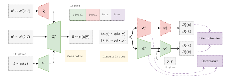
Figure 1: The overall structure of the GAN model. Federated modules are aggregated in each communication round, whereas private modules are not. The discriminative loss is just the GAN loss as described in Sec. 4.1, whereas the contrastive regularization term is explained in more detail in Sec. 4.3. We describe the model’s components in more detail in the supplementary material.

3.2 Generative Adversarial Networks (GANs)

Generative Adversarial Networks (GANs) [11] are powerful generative models that are well-known for their high-fidelity image generation capabilities [21] among other applications. The framework consists of two competing models playing a minimax game. The competing models are called the generator and the discriminator. The generator’s main objective is to generate samples so that they cannot be discriminated from real samples.

To put it formally, let the true distribution over the data be $q(\mathbf{x})$, the generative model $G:\mathcal{Z}\to\mathcal{X}$ and the discriminator $D:\mathcal{X}\to\mathbb{R}$, where $\mathcal{X}:=\mathbb{R}^{\text{height}\times\text{width}\times\text{depth}}$ is the image space and $\mathcal{Z}$ is the latent space. Further, let $p(\mathbf{z})$ be the latent distribution, which is typically standard normal $\mathcal{N}(0,I)$. Thus, the GAN objective can be written as $\min_{G}\max_{D}V(D,G)$ where

$$V(D,G)=\underset{q(\mathbf{x})}{\mathbb{E}}\log(D(\mathbf{x}))+\underset{p(\mathbf{z})}{\mathbb{E}}\log(1-D(G(\mathbf{z}))).$$ (2)

Conditional GANs. In general, we might want our model to make use of labels $\mathbf{y}$ in supervised data, so the space of data becomes $\mathcal{X}\times\mathcal{Y}$, where $\mathcal{Y}$ can be $\{0,1\}^{d_{y}}$ for a set of $d_{y}$ classes, for example. In our case, the label is a one-hot vector indicating one class at a time, so we also have $\sum_{j}y_{j}=1$. We can define a generative distribution over data in the previous equation as $p(\mathbf{x})=G(p(\mathbf{z}))$, so by adding labels we can get $p(\mathbf{x},\mathbf{y})=p(\mathbf{x}|\mathbf{y})p(\mathbf{y}):=G(p(\mathbf{z}),\mathbf{y})$. Then, we can rewrite the GAN objective above as follows

$$V(D,G)=\underset{q(\mathbf{y})}{\mathbb{E}}\underset{q(\mathbf{x}|\mathbf{y})}{\mathbb{E}}\log(D(\mathbf{x},\mathbf{y}))\\ +\underset{p(\mathbf{y})}{\mathbb{E}}\underset{p(\mathbf{x}|\mathbf{y})}{\mathbb{E}}\log(1-D(\mathbf{x},\mathbf{y})).$$ (3)

The method we adopt for conditioning the GAN is based on [35]. First, in the unconditional case, we can write $D(\mathbf{x})=(\mathcal{A}\circ\psi\circ\phi)(\mathbf{x})$ a decomposition of the discriminator, where $\mathcal{A}$ is the activation (e.g. $\mathcal{A}$ is the sigmoid function in 3), $\phi(\mathbf{x}):\mathcal{X}\to\mathcal{R}$ returns the hidden features of $\mathbf{x}$ (or as we will demonstrate later, the representation of $\mathbf{x}$), and $\psi:\mathcal{R}\to\mathbb{R}$, which is often a linear layer. Thus, $\psi(\phi(\mathbf{x}))$ can be thought of as the logit of $p(\mathbf{x})$, where $\text{logit}=\text{sigmoid}^{-1}$. In other words, $\psi(\phi(\mathbf{x}))$ is a real number that can be mapped to $[0,1]$ with the sigmoid function so that it represents a probability. Thus, the choice $\mathcal{A}=\text{sigmoid}$ implies $D(\mathbf{x})=p(\mathbf{x})$.

Then, the basic idea of adding a conditional variable $\mathbf{y}$ is to note that $p(\mathbf{x},\mathbf{y})=p(\mathbf{y}|\mathbf{x})p(\mathbf{x})$ and model $\log p(\mathbf{y}|\mathbf{x})$ as a simple log linear model

$$\log p(\mathbf{y}=y|\mathbf{x}):={(\bm{v}_{y}^{p})}^{\intercal}\phi(\mathbf{x})-\log Z(\phi(\mathbf{x})),$$ (4)

where $Z(\phi(\mathbf{x})):=\sum_{y^{\prime}\in\mathcal{Y}}\exp\left({(\bm{v}_{y^{\prime}}^{p})}^{\intercal}\phi(\mathbf{x})\right)$ is the partition function. The authors of [35] observed that the optimal solution of $D$ has the form of the ratio of the two log-likelihoods $D^{*}=\mathcal{A}(\log q^{*}(\mathbf{x},\mathbf{y})/\log p^{*}(\mathbf{x},\mathbf{y}))$ [11], and given the assumption that $D$ should follow the optimal form and the log linear model in 4, they reparameterized $D$ by absorbing the terms depending on $\mathbf{y}|\mathbf{x}$ and $\mathbf{x}$ separately to obtain an expression of the form

$$D(\mathbf{x},\mathbf{y})=\mathcal{A}\left(\mathbf{y}^{\intercal}V\phi(\mathbf{x})+\psi(\phi(\mathbf{x}))\right),$$ (5)

where $V$ is the embedding matrix of $\mathbf{y}$.

The choice $\mathcal{A}=\text{sigmoid}$ activation is used in the vanilla GAN objective, and $\mathcal{A}=\text{identity}$ used for the Wasserstein metric [13]. We use the latter in our implementation.

3.3 Self-Supervised Learning (SSL)

Self-supervised learning is a modern paradigm of learning in which the supervision is implicit, either by learning a generative model of the data itself or by leveraging some invariance in the data [31]. For example, we know that the label of an image is invariant to small translations and distortions. Such properties help for learning a low dimensional representation such that the labels, which are not used during training, are highly separable in this representation space, i.e. can be classified with high accuracy using a linear classifier. One well-known method is to use a contrastive objective [27], which simply pulls similar data together and pushes different data away. Knowing which data are similar and which are not is the part where implicit supervision happens. For example, data augmentations should result in similar data because the label should be invariant to augmentations.

We describe the general form of a contrastive loss, which includes InfoNCE [36] and NT-Xent [5]. Let $\phi$ be an encoder that takes data $\mathbf{x}$ and return its representation, and let $\mathbf{x}$ and $\mathbf{x}^{+}$ be two similar data. Then, given a similarity metric “sim”, such as the dot product, and $\tau$ a temperature (i.e. sensitivity) hyperparameter, we have

$$\mathcal{L}_{\text{contrast}}(\mathbf{x};\mathbf{x}^{+})=-\log\tfrac{e^{\text{sim}(\phi(\mathbf{x}),\phi(\mathbf{x}^{+}))/\tau}}{{\mathbb{E}}_{\mathbf{x}^{-}}[e^{\text{sim}(\phi(\mathbf{x}),\phi(\mathbf{x}^{-}))/\tau}]}.$$ (6)

The similarity metric is often a dot product taken after embedding the representations in some metric space via a learnable projection. For example, the projection can be parameterized as a one hidden layer neural net with a non-linearity.

Recently, many methods have been proposed to tackle the problem of mining negative samples (for computing the expectation in the denominator) by momentum-contrasting with a moving-average encoder [14] or by using stop gradient operator [6]. One technique of particular interest is Barlow Twins [48], which optimizes the empirical cross-correlation matrix of two similar representations to be as close to the identity matrix as possible, which should maximize correlation and minimizes redundancy, thus the name Barlow for his redundancy-reduction principle [3]. The empirical cross-correlation between two batches of projected representations $\mathbf{A}=g(\phi(\mathbf{x}))$ and $\mathbf{B}=g(\phi(\mathbf{x}^{+}))$ for some projection $g$ is defined as

$$\mathcal{C}(\mathbf{A},\mathbf{B})_{ij}=\tfrac{\sum_{b}\mathbf{A}_{b,i}\mathbf{B}_{b,j}}{\sqrt{\sum_{b}(\mathbf{A}_{b,i})^{2}}\sqrt{\sum_{b}(\mathbf{B}_{b,i})^{2}}}.$$ (7)

Now, the objective of Barlow Twins is

$$\mathcal{L}_{\text{BT}}(\phi(\mathbf{x}),\phi(\mathbf{x}^{+}))=\textstyle{\sum}_{i}(1-\mathcal{C}_{ii})^{2}+\lambda_{BT}\textstyle{\sum}_{i\neq j}\mathcal{C}_{ij}^{2},$$ (8)

where we omit the dependence of $\mathcal{C}$ on $g(\phi(\mathbf{x}))$ and $g(\phi(\mathbf{x}^{+}))$ for clarity. The hyper-parameter $\lambda_{BT}$ controls the sensitivity of the off-diagonal “redundancy” terms and is often much smaller than 1.

4 Partial Disentanglement with Partially-Federated GANs (PaDPaF)

In this section, we present a framework for Partial Disentanglement with Partially-Federated (PaDPaF) GANs, which aims at recovering the client invariant representation (the content) by disentangling it from the client-specific representation (the style). A contrastive regularization term is used to force the discriminator to learn a representation of some factor invariant to the variations of other factors, i.e. a content representation invariant to style latent variations given the same content latent, and similarly for the style representation.

4.1 Federated Conditional GANs

Starting from the GAN framework in Sec. 3.2, we aim to optimize 3 in the federated setting with respect to the parameters of $D_{i}$ and $G_{i}$ per client $i$. We define the generator to be a style-based generator with the architecture in [13], and a style vectorizer as in [21] for producing the conditioning variable of the conditional batch normalization layers [7]. The discriminator architecture is based on [15] with the addition of spectral normalization [34].

The style vectorizer is set to be private (i.e. unique to each client), while the base parameters of the generator are federated (i.e. shared). Also, in addition to the normal—or henceforth “content”—discriminator, we introduce another “style” discriminator in parallel, which is assumed to be client-specific with private parameters. This split is done so that we reserve the domain-specific parameters to be private and solely optimized by the clients’ optimizers, whereas the “content” parameters are federated and optimized collaboratively.

Namely, for each client $i$, we introduce $D_{i}^{c}(\mathbf{x},\mathbf{y}):\mathcal{X}\times\mathcal{Y}\to\mathbb{R}$, the content discriminator, and $D_{i}^{s}(\mathbf{x}):\mathcal{X}\to\mathbb{R}$ is the style discriminator. As for the generator, we let $G_{i}^{c}(\mathbf{z}_{i}^{c},G_{i}^{s}(\mathbf{z}_{i}^{s}),\mathbf{y}):\mathcal{Z}_{i}^{c}\times\mathcal{Z}_{i}^{s}\times\mathcal{Y}\to\mathcal{X}$, where $G_{i}^{s}:\mathcal{Z}_{i}^{s}\to{Z}_{i}^{s}$ is the style vectorizer. For simplicity, we assume that $D_{i}^{c}$ and $D_{i}^{s}$ have the same architectures, but this is not necessary. Let $\phi_{i}^{c}:\mathcal{X}\to\mathbb{R}^{d_{c}}$ for some content representation dimension $d_{c}$, and for simplicity, assume that the style representation dimension is the same $d_{s}=d_{c}$. Finally, let the parameters of $D_{i}^{c}$, $D^{s}$, $G_{i}^{c}$, and $G_{i}^{s}$ be $\theta_{i}^{c,D}$, $\theta_{i}^{s,D}$, $\theta_{i}^{c,G}$, and $\theta_{i}^{s,G}$, respectively. Then, we have $\theta_{i}^{\text{fed}}:=[\theta_{i}^{c,D};\theta_{i}^{c,G}]$ the federated parameters and $\theta_{i}^{\text{pvt}}:=[\theta_{i}^{s,D};\theta_{i}^{s,G}]$ the private parameters. We also introduce the shorthand $\theta_{i}^{D}=[\theta_{i}^{c,D};\theta_{i}^{s,D}]$ and $\theta_{i}^{G}=[\theta_{i}^{c,G};\theta_{i}^{s,G}]$. Now, we rewrite the client objective to follow the convention in 1

$$f_{i}(\theta;\xi)=\underset{\mathbf{x},\mathbf{y}\in\xi}{\mathbb{E}}\left[\log(D_{i}^{c}(\mathbf{x},\mathbf{y})+\log(D_{i}^{s}(\mathbf{x}))\right]+\\ \underset{\tilde{\mathbf{x}},\tilde{\mathbf{y}}\in p_{i}(\cdot;\theta)}{\mathbb{E}}\left[\log(1-D_{i}^{c}(\tilde{\mathbf{x}},\tilde{\mathbf{y}}))+\log(1-D_{i}^{s}(\tilde{\mathbf{x}}))\right].$$ (9)

We make the dependence on $\theta$ explicit for the generative model $p_{i}$ since $p_{i}(\tilde{\mathbf{x}},\tilde{\mathbf{y}};\theta)=G_{i}^{c}(\mathbf{z}_{i}^{c},G_{i}^{s}(\mathbf{z}_{i}^{s}),\tilde{\mathbf{y}})$ where $\mathbf{z}_{i}^{c}$, $\mathbf{z}_{i}^{s}$ are standard Gaussian, i.e. $\mathbf{z}^{c},\mathbf{z}^{s}\sim\mathcal{N}(0,I)$ and $\tilde{\mathbf{y}}$ is drawn randomly from $\mathcal{Y}$. We make the dependence on $\theta$ implicit elsewhere, making the objective less convoluted.

4.2 Partially-Federated Conditional GANs

When the client’s data distributions are not iid—which is clearly the case in practice—then we can have a confounding variable, which is the client’s domain variable $i$. In our case, we assume that each client has its own domain and unique variations. In practice, especially when we have hundreds of millions of clients, meta-data can be used to cluster clients into similar domains. The implementation of this idea will be left for future work.

Before we proceed, we make a simplifying assumption about the content of $\mathbf{y}$.

Assumption 1 (Independence of content and style)

Given an image $x\sim q(\mathbf{x})$, the label $\mathbf{y}$ is independent from $i$, i.e. $\mathbf{y}$ should contain no information about $i$ given $\mathbf{x}$. Namely,

$$q_{i}(\mathbf{y}|\mathbf{x})=q(\mathbf{y}|\mathbf{x}).$$ (10)

It is worth mentioning that this assumption might not be entirely true in practice. Take, for example, the case with MNIST, where some client writes 1 and 7 very similar to each other, and another client also writes 1 in the same way but always writes a 7 with a slash, so it is easily distinguishable from a 1. Then, a sample of the digit 7 without a slash would be hard to distinguish from a 1 for the first client but easily recognizable as a 1 for the second client. Hence, given $\mathbf{x}$, there could be some information in the dependence $\mathbf{y}|\mathbf{x}$ that would allow us to discriminate the domain $i$ from which $\mathbf{x}$ came from. However, we do not concern ourselves with such edge cases and make the simplifying assumption that the global representation of the content of $\mathbf{x}$ should be, in theory, independent from the local variations introduced by the client.

Given this assumption, we would like to construct our base generative model such that $p_{i}(\mathbf{y}|\mathbf{x}):=p(\mathbf{y}|\mathbf{x},i)$ is invariant to $i$ and $p_{i}(\mathbf{x})=p(\mathbf{x}|i)$ generates personalized data from domain $i$. First, we let $p(i)$ the probability of sampling client $i$, which we assume to be uniform on the clients, and $p(\mathbf{y})$ the prior of the labels, which we also assume to be uniform on the labels. Note here that the label distribution for a given $i$ could be disjoint or has a small overlap with different $i$’s. This is particularly true in practice, as clients rarely have access to all possible labels for a specific problem. More importantly, it implies that $\mathbf{x}$ can depend non-trivially on $i$ as well (e.g. through data augmentations, see our construction in Fig. 4). However, we want our model to be agnostic to the client’s influence on $\mathbf{y}|\mathbf{x}$ for a globally-consistent inference while being specific to its influence on $\mathbf{x}$ for a personalized generation.

As for $p_{i}(\mathbf{y}|\mathbf{x})$, we enforce the independence of $\mathbf{y}|\mathbf{x}$ from $i$ via a split of private and federated parameters. This split should influence the mechanism of the generative latent variables $\mathbf{z}_{i}^{c}$ and $\mathbf{z}_{i}^{s}$ of $\mathbf{x}$, so that $\mathbf{z}^{c}$’s generative mechanism becomes increasingly independent of $i$ as we run federated averaging on it, while $\mathbf{z}^{s}$’s generative mechanism is private and depends on $i$. The causal model we assume is shown in Fig. 2, and the idea of the independence of mechanisms is inspired by [12].

Figure 2: A causal model with the generative latent variables $\mathbf{z}^{c}$ and $\mathbf{z}^{s}$ of $\mathbf{x}$. The dotted arrows show the underlying causal model without latents. Both latents depend on the client $i$, and we assume that the content latent $\mathbf{z}^{c}$ generates the label $\mathbf{y}$ as well. The blue arrows drop when we $do(\mathbf{z}^{c})$, and the red arrows drop when we $do(\mathbf{z}^{s})$. The dashed arrows indicate the reduced influence of $i$ over $\mathbf{z}^{c}$ as we run federated averaging. $\mathbf{z}^{s}$ and its mechanism, on the other hand, are specific to the client in our case.

We can write the full probability distribution as $p(\mathbf{y}|\mathbf{z}^{c})p(\mathbf{x}|\mathbf{z}^{c},\mathbf{z}^{s})p(\mathbf{z}^{c}|i)p(\mathbf{z}^{s}|i)p(i)$. Assuming an optimal global solution for all $\theta_{i}^{c}\to\theta^{c,\star}$ exists as well as local optimal solutions $\theta_{i}^{s,\star}$, and assuming they are attainable with federated learning on (9), we have that

$$p_{i}(\mathbf{y}|\mathbf{x})\overset{t\to\infty}{\longrightarrow}p(\mathbf{y}|\mathbf{z}^{c})p(\mathbf{z}^{c}|\mathbf{x};\theta^{c,\star})p_{i}(\mathbf{z}^{s}|\mathbf{x};\theta_{i}^{s,\star}).$$ (11)

Now, we have the problem of “inverting the data generating process” $p(\mathbf{z}^{c}|\mathbf{x};;\theta_{i}^{c})$ and $p_{i}(\mathbf{z}^{s}|\mathbf{x};\theta_{i}^{s})$. We will next show how we can disentangle the content latent from the style latent using a contrastive regularizer on the discriminators, inspired by recent results in contrastive learning [50].

4.3 Contrastive Regularization Between Federated and Private Representations

The main motivation for partitioning our model into federated and private components is that the federated components should be biased towards a solution invariant to the client. This is a desirable property to have for predicting $\mathbf{y}$ given $\mathbf{x}$. However, from a generative perspective, we still want to learn $\mathbf{x}$ given $\mathbf{y}$ and $i$, so we are interested in learning a personalized generative model that can model the difference in changing the client $i$ while keeping $\mathbf{x}$ and $\mathbf{y}$ fixed, and similarly change $x$ while keeping $i$ fixed. This type of intervention can help us understand how to represent these variations better.

Assume for now that we do not have $\mathbf{y}$. We want to learn how $i$ influences the content in $\mathbf{x}$. The variable $i$ might have variations that correlate with the content, but the variations that persist across multiple clients should be the ones that can potentially identify the content of the data. From another point of view, a datum with the same content might have a lot of variations within one client. Still, if these variations are useless for another client, we should not regard them as content-identifying variations. Thus, our proposed approach tries to maximize the correlation between the content representation between two generated images with the same content latent. This is also applied analogously to style. To achieve that, we use the Barlow Twins objective (8) as a regularizer and the generator as a model for simulating these interventions. Indeed, such interventional data are almost impossible to come by in nature without simulating the generative process.

First, let $g$ be a projector from the representation space to the metric embedding space, and let us denote a shorthand for the embedding of the $\#$-discriminator representation of a sample from the generator as $\Phi_{i}^{\#}(\mathbf{z}^{c},\mathbf{z}^{s};\mathbf{y})=g_{i}\left(\phi_{i}^{\#}((\text{sg}[G_{i}^{c}(\mathbf{z}^{c},G_{i}^{s}(\mathbf{z}^{s}),\mathbf{y})])\right)$, where $\#\in\{c,s\}$ and sg is a stop gradient operator to simulate a sample from the generative model without passing gradients to it. Omitting $\mathbf{y}$ for clarity, the Barlow Twins regularizer will then be

$$\Gamma_{i}(\theta)=\underset{\mathbf{z}^{c},\mathbf{z}^{s},\tilde{\mathbf{z}}^{c},\tilde{\mathbf{z}}^{s}}{\mathbb{E}}[\mathcal{L}_{\text{BT}}\left(\Phi_{i}^{s}(\mathbf{z}^{c},\mathbf{z}^{s}),\Phi_{i}^{s}(\mathbf{z}^{c},\tilde{\mathbf{z}}^{s})\right)\\ +\mathcal{L}_{\text{BT}}\left(\Phi_{i}^{c}(\mathbf{z}^{c},\mathbf{z}^{s}),\Phi_{i}^{c}(\tilde{\mathbf{z}}^{c},\mathbf{z}^{s})\right)].$$ (12)

The intuition here is that the correlation of the content representation between two images generated by fixing the content latent and changing other variables should be exactly the same, and similarly for the style and other components if any. This is related to the intervention concept in causal inference [37], and assuming the generator is optimal, we can simulate a real-world intervention and self-supervise the model by a contrastive regularization objective as in (12). If we let $\mathcal{L}_{\text{BT}}^{\#}(\mathbf{x}_{1},\mathbf{x}_{2})=\mathcal{L}_{\text{BT}}\left(g_{i}(\phi_{i}^{\#}(\mathbf{x}_{1})),g_{i}(\phi_{i}^{\#}(\mathbf{x}_{2}))\right)$ the consistency regularizer from the #-discriminator’s perspective, then we can rewrite the objective in terms of interventions on the generator’s latent variables as

$$\tilde{\Gamma}_{i}(\theta,\mathbf{z}^{c},\mathbf{z}^{s}) =\underset{\begin{subarray}{c}\tilde{\mathbf{z}}^{s}\sim\\ p(\mathbf{z}^{s})\end{subarray}}{\mathbb{E}}\underset{\begin{subarray}{c}\mathbf{x}_{1},\mathbf{x}_{2}\sim\\ p(\mathbf{x}|\tilde{\mathbf{z}}^{s},do(\mathbf{z}^{c}))\end{subarray}}{\mathbb{E}}\mathcal{L}^{c}_{\text{BT}}(\mathbf{x}_{1},\mathbf{x}_{2})$$

$$+\underset{\begin{subarray}{c}\tilde{\mathbf{z}}^{c}\sim\\ p(\mathbf{z}^{c})\end{subarray}}{\mathbb{E}}\underset{\begin{subarray}{c}\mathbf{x}_{1},\mathbf{x}_{2}\sim\\ p(\mathbf{x}|\tilde{\mathbf{z}}^{c},do(\mathbf{z}^{s}))\end{subarray}}{\mathbb{E}}\mathcal{L}^{s}_{\text{BT}}(\mathbf{x}_{1},\mathbf{x}_{2}),$$ (13)

$$\Gamma_{i}(\theta) =\underset{\mathbf{z}^{c},\mathbf{z}^{s}\sim p(\mathbf{z}^{c},\mathbf{z}^{s})}{\mathbb{E}}[\tilde{\Gamma}_{i}(\theta,\mathbf{z}^{c},\mathbf{z}^{s})].$$ (14)

Thus, we can write the regularized client objective as

$$F_{i}(\theta;\lambda)=\underset{\xi\sim\mathcal{D}_{i}}{\mathbb{E}}[f_{i}(\theta;\xi)]+\lambda\Gamma_{i}(\theta).$$ (15)

See Fig. 2 for a clearer understanding of the interventions.

Implementation details. The algorithm for training our model is a straightforward implementation of GAN training in a federated learning setting. We use FedAvg [33] algorithm as a backbone for aggregating and performing the updates on the server. The main novelty stems from combining a GAN architecture that can be decomposed into federated and private components, as depicted in Fig. 1, with a contrastive regularizer (12) for the discriminator in the GAN objective. The training algorithm and other procedures are described in more detail in Appendix A.

5 Experiments

We run the basic experiments that showcase our model capabilities on MNIST [28]. We also provide experiments for CelebA [32] to show the robustness and generalization of our model in Appendix C. More experimental details can be found in the supplementary material. We generally use Adam [22] for both the client’s and the server’s optimizer.

The types of experiments are divided as follows. Firstly, we show how our generator disentangles content from style visually. Then, we show how the generator can generate locally-unseen labels or attributes, i.e. generate samples from the client’s distribution given labels or attributes that the client has never seen. Next, we show how the representation learned by the content discriminator contains sufficient information so that a simple classifier on it yields high accuracy on downstream tasks.
MNIST.

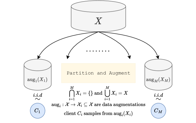
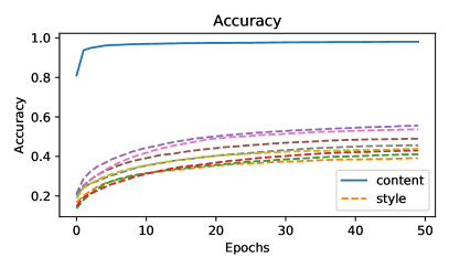
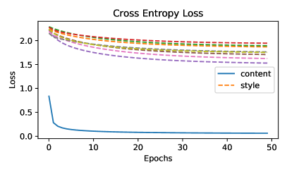
Figure 3: Preparation of our federated MNIST dataset. Note that the more clients there are, the fewer data each client will get.

Figure 4: Accuracy and loss of a linear classifier on the content and style representations of an unconditional GAN on MNIST’s test set. The final accuracy is 98.1%.

In our MNIST experiments, we generate a federated dataset by partitioning MNIST equally on all clients and then adding a different data augmentation for each client. This way, we can test whether our model can generate global instances unseen to the client based on its own data augmentation. The data augmentations in the figures are as follows (in order): 1) zoom in, 2) zoom out, 3) colour inversion, 4) Gaussian blur, 5) horizontal flip, 6) vertical flip, 7) rotation of at most 40 degrees, and 8) brightness jitter.

See Figs. 6 and 6 for samples from an unconditional GAN, and Figs. 8 and 8 for samples from a conditional GAN. One interesting observation about the samples in Figs. 8 and 8 is that, since the number 7 was seen only in the horizontally flipped client, it retains this flipped direction through other clients as well. This is not a bug in our model but a feature. In general, learning flipping as a style does not seem to be easy. Also, rotations were not really learned as style (see Fig. 8, lower left). However, the content was generally preserved through most other clients. We show performance on other more difficult augmentations in Appendix C.
Finally, Fig. 4 shows that the content representation has sufficient information such that a linear classifier can achieve of 98.1% accuracy on the MNIST test set. It is also clear that the style representations do not contain as much information about the content. This empirically confirms that our method can capture the most of $\mathbf{z}^{c}$ and disentangle it from $\mathbf{z}_{i}^{s},\forall i$.

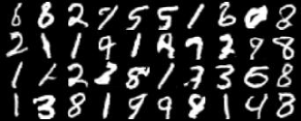
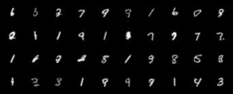
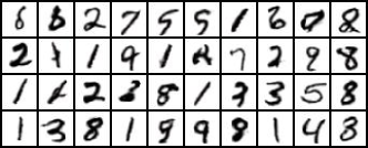
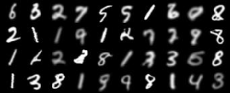
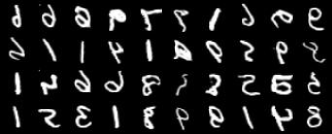
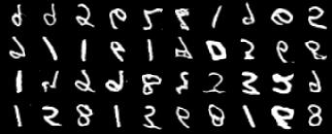
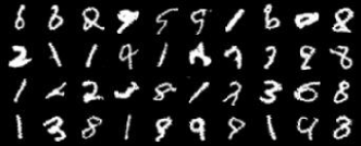
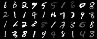
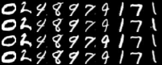
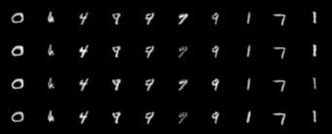
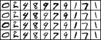
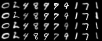
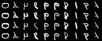
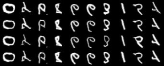
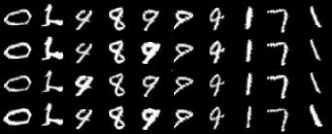
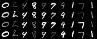
Figure 5: Samples from an unconditional GAN using different content and style latent for all cells per client.

Figure 6: Samples from an unconditional GAN using the same content latent per row and a different style latent for all cells per client.

CelebA. We provide experiments for CelebA in Appendix C. The federated dataset is created by a partition based on attributes. Given 40 attributes and 10 clients, each client is given 4 unique attributes, which all of its data have. The content part should then capture the general facial structures, and the style should capture the other non-global variations. Our results again confirm the empirical feasibility of our model.

6 Discussion

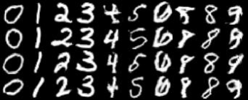
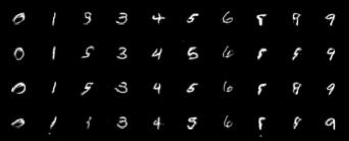
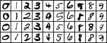
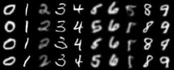
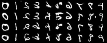
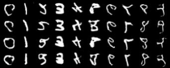
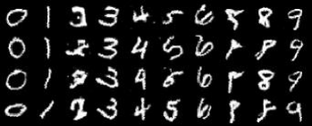
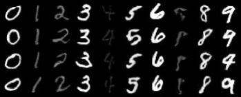
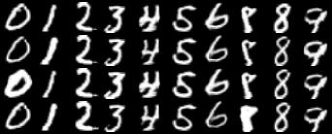
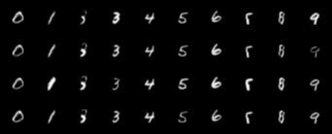
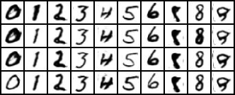
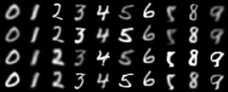
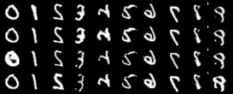
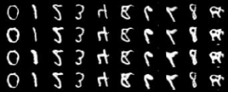
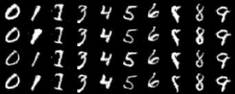
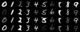
Figure 7: Samples from a conditional GAN using a different content latent for all cells and the same style latent per row per client.

Figure 8: Samples from a conditional GAN using the same content latent per row and a different style latent for all cells per client.

Our framework leaves some room for improvements and further work to be done in multiple directions. Here, we discuss some of those directions and highlight interesting aspects we can exploit.
Real-World Performance. How would our model perform in the real world? How can we increase its adaptability to end devices? For example, we can apply ordered dropout [17] on the federated part. Exploring this direction would be an important next step.
Decentralized training. We can easily extend our model to the decentralized setting, but understanding how to exploit or work around this less-constrained setting would be challenging, as the network topology might hinder progress in a non-trivial manner.
Client shift. Our architecture adapts to different clients $i$ under covariate shift $q_{i}(\mathbf{x})$ and prior shift $q_{i}(\mathbf{y})$. Can we extend it to the case of temporal heterogeneity? For example, our model might not work well with clients with diurnal activity.
Model improvement. How can we design a generator that can effectively incorporate clients’ variations? What about different modalities of data, such as language and sensorimotor control? Can we use an attention-based mechanism for controlling the aggregation or sampling mechanisms for our model? Further experimentation with more modern models within our framework would be interesting.
Privacy. The federated part of the generator of our model can stay in the server, but the federated discriminator needs direct access to the data in the client. Can we avoid that and just get some statistic or feature from the data that is sufficient for training our model? This would really improve the privacy of our model.
Conclusion. We introduced a framework combining federated learning, generative adversarial learning, and (causal) representation learning together by leveraging the federated setting for learning a client-invariant representation based on a causal model of the data-generating process, which we model as a GAN. We disentangle the content and style latents using a contrastive regularizer on the discriminator. Experiments validate our framework and show that our model is effective at personalized generation and self-supervised classification and benefits further from supervised data when available.

Appendix A Algorithm

In this section, we write the training algorithm in detail for completeness. The training is a straightforward application of FedAvg on GANs without its private parameters.

Algorithm 1 Contrastive GANs with Partial FedAvg

1:Input: Clients $i\in[M]$, datasets $X_{i}=\{(\mathbf{x}_{j},\mathbf{y}_{j})\}_{j=1}^{|X_{i}|}$, target distribution $q(\cdot|i)q(i)$ over $X_{i}$, GAN models $p_{i}(\cdot;\theta_{i})$, GAN objectives $f_{i}$, server and clients first-order optimizers $\textsc{Opt}_{0}$ and $\textsc{Opt}_{i}$ with step sizes $\eta_{0}$ and $\eta_{i}$, client’s loop stopping probability $\pi_{i}\propto|X_{i}|^{-1}$, and $T_{D}$ iterations for training $D$ vs. $G$.

2:Output: $\theta_{0}^{\text{fed}}$ and $\theta_{i}^{\text{pvt}},\forall i$.

3:Set $\theta_{i}:=\theta_{0}$, $\forall i\in[M]$

4:for $\tau=1,\cdots,\tau_{\text{max}}$ do

5:     Sample subset of clients $I\sim q(i)$

6:     for $i\in I$ in parallel do

7:         for $t=1,\cdots,t_{\text{max}}$ do

8:              $\text{train}_{G}\leftarrow\mathbbm{1}[t\bmod T_{D}+1=0]$

9:              $\theta_{i}(t+1)\leftarrow\textsc{GANOpt}\left(i,\theta_{i}(t),\text{train}_{G};f_{i},q_{i}\right)$

10:              if $1\sim\text{Bernoulli}(\pi_{i})$ then

11:                  $\Delta_{i}\leftarrow\theta_{i}(1)-\theta_{i}(t)$

12:                  $\Delta_{i}^{\text{pvt}}\leftarrow 0$

13:                  break loop

14:              end if

15:         end for

16:     end for

17:     $\theta_{0}(\tau+1)\leftarrow\textsc{Opt}_{0}\left(\frac{1}{|I|}\sum_{i\in I}\Delta_{i};\,\theta_{0}(\tau),\eta_{0}\right)$

18:     $\theta_{i}^{\text{fed}}\leftarrow\theta_{0}^{\text{fed}}$ for all clients $i\in[M]$

19:end for

20:procedure GANOpt($i$, $\theta_{i}$, $\text{train}_{G};f_{i},q_{i}$)

21:     if $\text{train}_{G}$ then

22:         return $\textsc{Opt}_{i}\left(\nabla_{\theta_{i}^{G}}f_{i}(\theta_{i},\cdot);\,\theta_{i},\eta_{i}\right)$

23:     else

24:         Sample $\xi\sim q(\cdot|i)$

25:         return $\textsc{Opt}_{i}\left(-\nabla_{\theta_{i}^{D}}f_{i}(\theta_{i},\xi);\,\theta_{i},2\eta_{i}\right)$

26:     end if

27:end procedure

Here, we let $\textsc{Opt}(\theta,\nabla f(\theta))$ be a first-order optimizer, such as SGD or Adam, that takes the current parameters $\theta$, and the gradient $\nabla f(\theta)$ and returns the updated parameters given step size $\eta$. We also define a subroutine GANOpt that runs a single descent or ascent step on the GAN’s objective. The term $\text{train}_{G}$ is a boolean variable that specifies whether the generator or the discriminator should be trained. In the GAN literature, the discriminator is often trained 3 to 5 times as much as the generator. In our experiments, we let $T_{D}=3$, so $D$ is trained 3 times before $G$ is trained, but we also update $\theta^{D}$ with double the learning rate, following the Two Time-scale Update Rule. As for the client’s loop, we can simply train it on the dataset for one epoch before breaking the loop so that $t_{\text{max}}=|X_{i}|$ and $\pi_{i}=0$, but we add a loopless option as well by letting $t_{\text{max}}=\infty$ and $\pi_{i}\propto|X_{i}|$ for the same training behaviour on average.

Note that we could have removed line 12 of the algorithm and let line 11 be $\Delta_{i}^{\text{fed}}\leftarrow\theta_{i}^{\text{fed}}(1)-\theta_{i}^{\text{fed}}(t)$, but we chose the current procedure to emphasize that the server’s update on the private parameters is always set to 0.

Appendix B Model Architecture

Our model’s architecture is composed of regular modules that are widely used in the GAN literature. The generator is a style-based generator with a ResNet-based architecture [13], where we use a conditional batch normalization layer [7] to add the style, which is generated via a style vectorizer [21]. The discriminator’s architecture is ResNet-based as well [15] with the addition of spectral normalization [34]. In the case of conditioning on labels, we follow the construction of the projection discriminator as in [35], so we add an embedding layer to the discriminator, and we adjust the conditional batch normalization layers in the generator by separating the batch into two groups channel-wise, and condition each group separately. Finally, we add a projector to the discriminator for contrastive regularization, which is a single hidden layer ReLU network. Recall that we use two discriminators, one is private, and the other is federated.

The variables that control the size of our networks are the image size, the discriminator’s feature dimension, and the latent variables’ dimension. We make the dimension of the content and style latent variables equal for simplicity. For MNIST, we choose the feature dimension to be 64 and the latent dimension to be 128. For CelebA, we choose the feature dimension to be 128 and the latent dimension to be 256. Kindly refer to the code for more specific details.

Appendix C Experiments

In this section, we describe the experiments we run in more detail and show results extra results supporting our framework.

For all our experiments, the client models are handled by “workers”. The workers only train their models on a specific subset of clients that does not change. We often assign a worker for each client, but due to constraints on computational resources, we might create a smaller number of workers and assign a specific subset of clients for each worker. We run all experiments on a single NVIDIA A100 SXM GPU 40GB.

Our choice for all the optimizers, including the server’s optimizer, is Adam [22] with $\beta_{1}=0.5$ and $\beta_{2}=0.9$. We choose Adam due to its robustness and speed for training GANs. We found that choosing learning rates 0.01 and 0.001 for the server optimizer and the client optimizer, respectively, is a good starting point. We also use an exponential-decay learning rate schedule for both the server and the clients, with a decay rate of 0.99 for MNIST (0.98 for CelebA) per communication round. This can help stabilize the GAN’s output.

C.1 MNIST

The MNIST train dataset is partitioned into 8 subsets assigned to 8 clients, and each client is handled by a unique worker. The data augmentations used for each partition are clear from the images. We write the PyTorch code for each data augmentation:

1. Zoom in: CenterCrop(22).

2. Zoom out: Pad(14).

3. Color inversion: RandomInvert(p=1.0).

4. Blur: GaussianBlur(5, sigma=(0.1, 2.0)).

5. Horizontal flip: RandomHorizontalFlip(p=1.0).

6. Vertical flip: RandomVerticalFlip(p=1.0).

7. Rotation: RandomRotation(40).

8. Brightness: ColorJitter(brightness=0.8).

In the case of conditioning on $\mathbf{y}$, we further restrict the datasets and drop 50% of the labels from each partitioned dataset. This implies that some data will be lost, and each client will see only 50% of the labels. This is intentional as we want to restrict the dataset’s size further and test our model’s robustness on unseen labels.

The results for training our model on this federated dataset are shown in Figs. 6 and 6 for the unconditional case (i.e. $\mathbf{y}$ is unavailable), and Figs. 8 and 8 for the conditional case with 50% labels seen per client. The results were generated after training the model for 300 communication rounds. For MNIST, we train the models for a half epoch in each round to further restrict the local convergence for each client.

C.1.1 Adaptation to New Clients (i.e. Data Augmentation)

After training our conditional model on the previous data augmentations, we re-train it for 25 communication rounds on the following data augmentations and show the results:

1. Affine: RandomAffine(degrees=(30, 70), translate=(0.1, 0.3), scale=(0.5, 0.75)).

2. Solarize: RandomSolarize(threshold=192.0).

3. Erase: transforms.RandomErasing(p=1.0, scale=(0.02, 0.1)) (after ToTensor()).

This is to show that our conditional model can quickly adapt to new styles without severely affecting its content generation capabilities and its generalization to unseen labels.

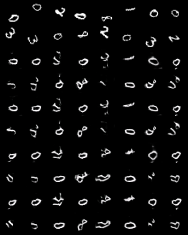
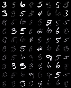
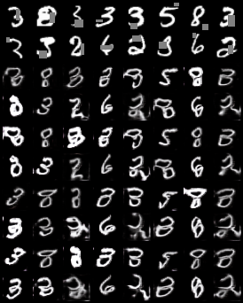
Figure 9: Results after re-training for 1 communication round on the three new data augmentations. Rows 1-2 are real samples and rows 3-8 are generated. Rows 3-6 share the same $\mathbf{z}^{c}$, and rows 7-10 as well. Rows 3-4 and 7-8 share the same $\mathbf{z}^{s}$, similarly for rows 5-6 and 9-10.

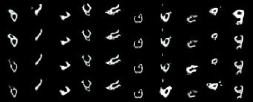
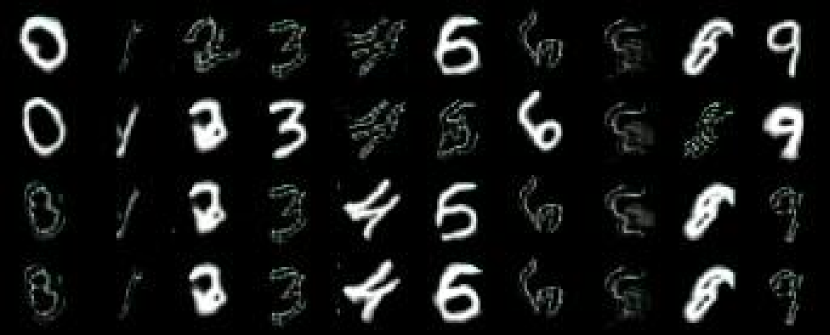
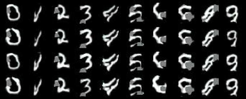
(a) Changing $\mathbf{z}^{s}$ per row while fixing $\mathbf{z}^{c}$.

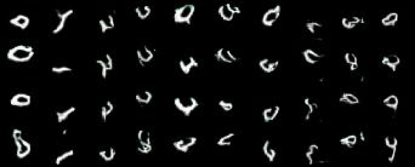
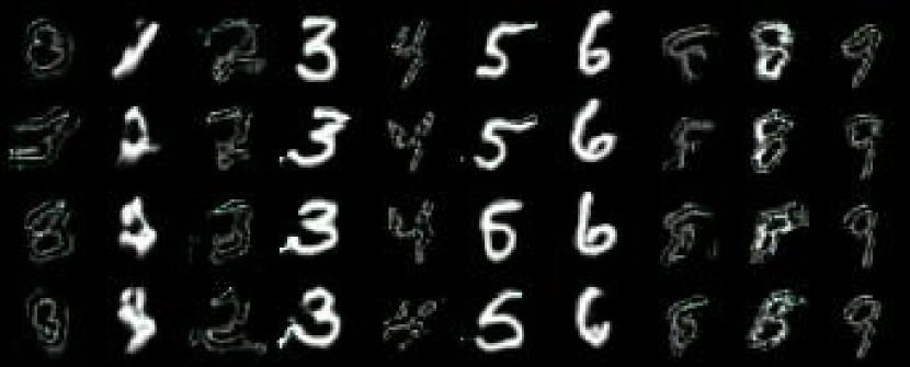
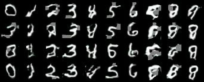
(b) Changing $\mathbf{z}^{c}$ per row while fixing $\mathbf{z}^{s}$.

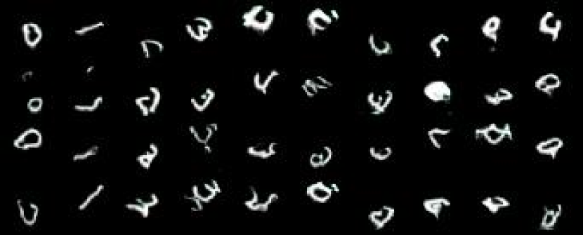
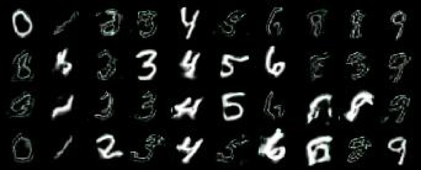
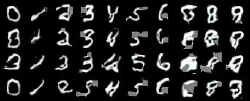
(c) Changing both $\mathbf{z}^{c}$ and $\mathbf{z}^{s}$.

Figure 10: Results after 25 communication rounds. We can see that solarization is learned as a style, while erosion is learned as a content. The generalization to unseen digits is maintained but less so in the challenging affine augmentation.

C.1.2 Can We Predict the Client from the Image?

We ask a question analogous to the one we are concerned with in representation learning. Instead of predicting the label from the image, we want to predict the augmentation, or the client, that generated the image. We show that we can predict the client with good accuracy (93.3%). See Fig. 11.

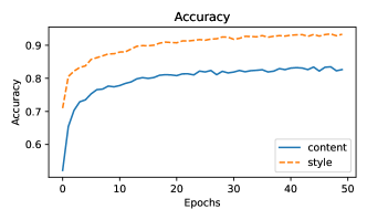
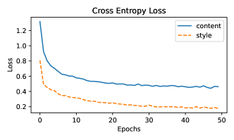
Figure 11: Prediction of style. We see that the content features have good accuracy (82.6%), but the style features can classify the source client with much better accuracy (93.3%).

The style prediction is done by linear transformations on the content representation and the style representations. For the style representations, we linearly map each representation from each client to a scalar $u_{i}$, so that $\bm{u}$ is a vector of all the scalars. We then pass $\bm{u}$ through an extra linear transformation to get a vector of logits for $p(i|\mathbf{x})$. Note that this is still a linear transformation of the style representations, but we do it this way to reduce dimensionality.

Note that the content representation can still predict the style with good accuracy. Indeed, we have seen that our generator architecture finds difficulties in assigning rotations to style variations, which is due to the style generator construction as a conditional batch normalization layer, which shows limited capabilities in capturing rotation-like variations. Still, the prediction accuracy from the style representations is better overall, which shows that our model does disentangle, to some extent, the style from the content.

C.1.3 Re-Styling via Content Transfer

We describe a simple method for transferring the content of an image to another style, given the style vectorizers $G_{i}^{s}$. In other words, we can transfer the content of an image taken from one client to another without sharing the image but by finding the approximate latent variables that generate the image and transferring the content latent variable. We shall see that this approach can indeed transfer the content well enough, where the content is up to the generator’s expressiveness and its separation of style. For example, we show that our generator finds difficulties in distinguishing some rotations as non-content variations. This is because all other clients have slightly rotated digits as well.

To find the approximate latent variables from the image without any significant overhead, we use the discriminator’s representations to predict the latent variables. We show that this approach can predict latents that reconstruct the image very well, and thus we can use the same content latent on the new client.

Algorithm 2 Re-style via content transfer

1:Input: Trained models, $t_{\text{max}}$ number of epochs, $\mathbf{x}_{a}$ (and $\mathbf{y}_{a}$, if any) a sample from source client $a$, and a target client $b$.

2:Output: Representation-to-latent transforms $\mathfrak{Z}^{c}$ and $\mathfrak{Z}_{i}^{s}$ for each $D_{0}^{c}$ and $D_{i}^{s}$, resp., $\forall i\in[M]$, and re-styled $\mathbf{x}_{b}$.

3:for $t=1,\cdots,t_{\text{max}}$ do

4:     Sample client $i\sim q(i)$, and sample label $\mathbf{y}\sim q_{i}(\mathbf{y})$, if any.

5:     Sample latents $\mathbf{z}^{c}\sim q_{i}(\mathbf{z}^{c})$ and $\mathbf{z}^{s}\sim q_{i}(\mathbf{z}^{s})$.

6:     Sample image $\mathbf{x}\sim p_{i}(\mathbf{x}|\mathbf{z}^{c},\mathbf{z}^{s},\mathbf{y})$ (i.e. set $\mathbf{x}=G_{0}^{c}(\mathbf{z}^{c},G_{i}^{s}(\mathbf{z}^{s}),\mathbf{y})$).

7:     Transform latents $\tilde{\mathbf{z}}^{c}=\mathfrak{Z}^{c}(\phi_{0}^{c}(\mathbf{x}))$ and $\tilde{\mathbf{z}}_{i}^{s}=\mathfrak{Z}_{i}^{s}(\phi_{i}^{s}(\mathbf{x}))$.

8:     Sample reconstructed image $\tilde{\mathbf{x}}\sim p_{i}(\mathbf{x}|\tilde{\mathbf{z}}^{c},\tilde{\mathbf{z}}^{s},\mathbf{y})$.

9:     Minimize $\mathcal{L}_{\text{BT}}(\phi_{0}^{c}(\mathbf{x}),\phi_{0}^{c}(\tilde{\mathbf{x}});g_{0}^{c})$ w.r.t. $\mathfrak{Z}^{c}$ and $\mathfrak{Z}_{i}^{s}$ (see (8)).

10:end for

11:Transfer $a\to b$: Sample $\mathbf{x}_{b}\sim p_{b}(\mathbf{x}|\mathfrak{Z}_{0}^{c}(\phi_{0}^{c}(\mathbf{x}_{a})),\mathbf{z}_{b}^{s},\mathbf{y}_{a})$, where $\mathbf{z}_{b}^{s}\sim p_{b}(\mathbf{z}^{s})$.

First, we show the algorithm for reconstructing and re-styling an image from some client. The main idea is to use $\mathcal{L}_{\text{BT}}$ from (8) to maintain an identity correlation between the source content representation and the target (i.e. reconstructed) content representation. We noticed that we do not need to do the same for the style representation. In fact, not enforcing an identity correlation between styles can even improve the results in terms of style consistency. We do not find a good explanation for this. We believe that applying Barlow Twins loss in our setting warrants further empirical and theoretical investigation.

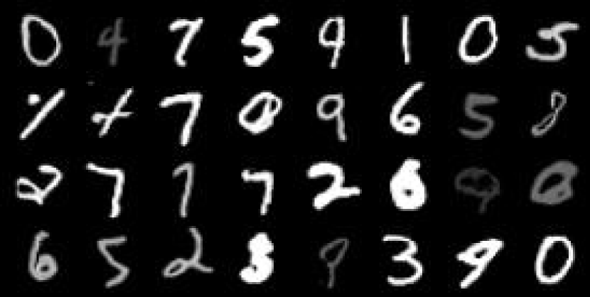
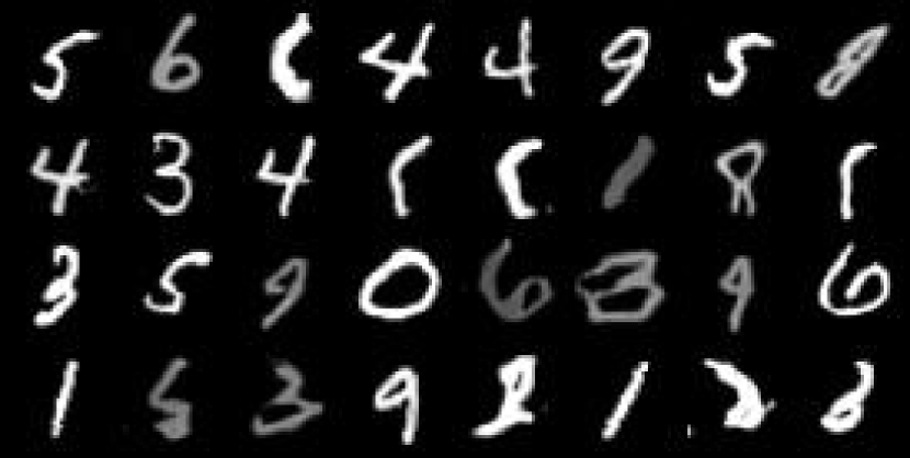
(a) Source (generated) images.

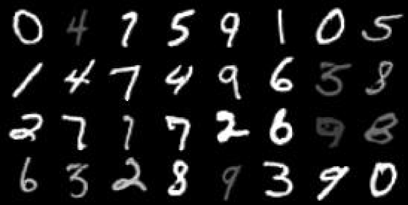
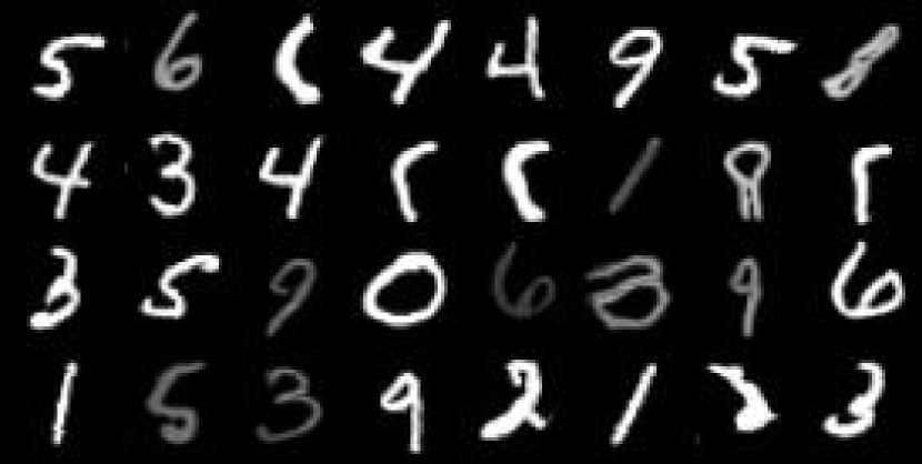
(b) Reconstructed images.

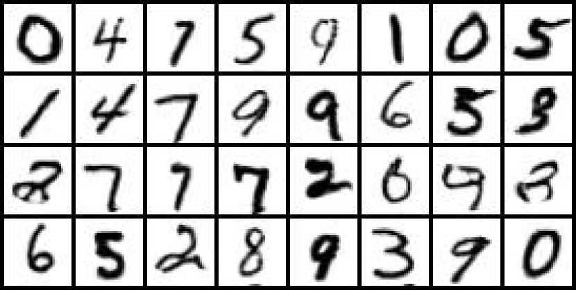
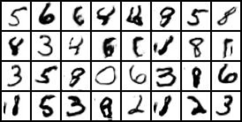
(c) Re-styled with transferred content.

Figure 12: The images show results from the regular, unconditional GANs, whereas the bottom show results for conditional GANs with 50% labels seen per client. Observe how the content stays preserved after transfer. Here, we show an example of transferring the content from client 8 (brightness) to client 3 (color inversion).

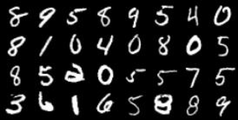
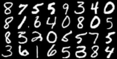
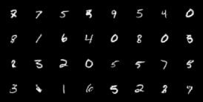
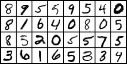
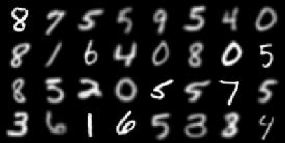
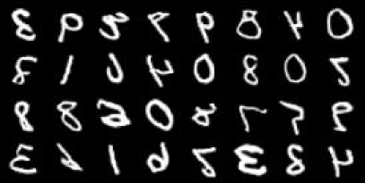
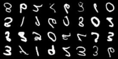
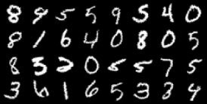
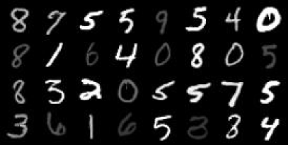
(a) Unconditional.

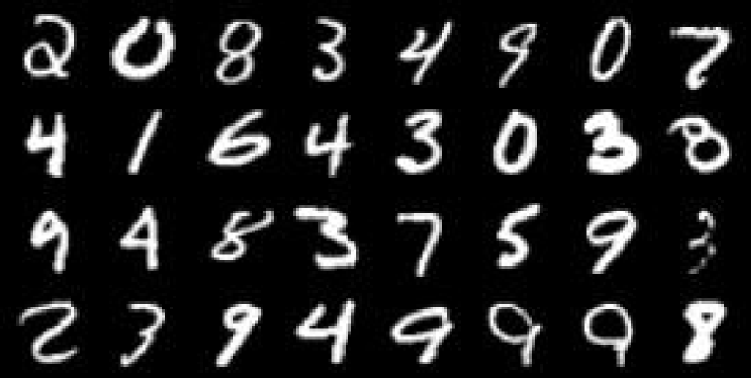
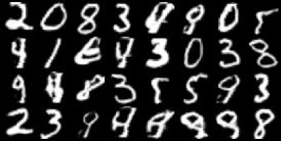
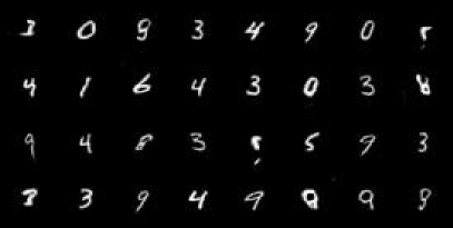
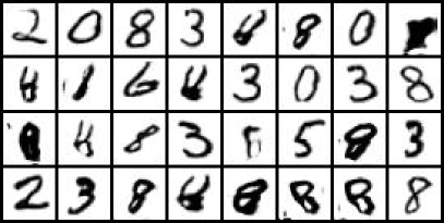
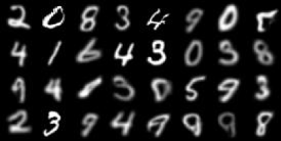
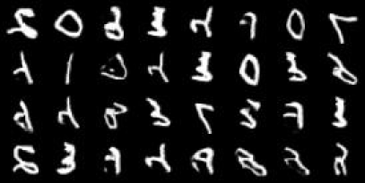
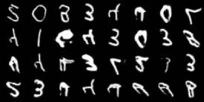
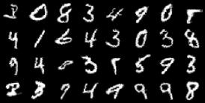
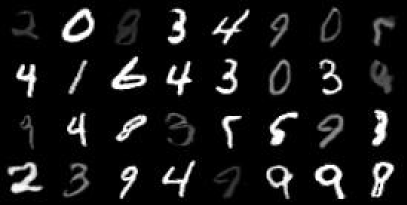
(b) Conditional, 50% labels per client.

Figure 13: Transferring an image from MNIST’s test set to all clients. Test image on top transferred image to each client at the bottom.

The effectiveness of this procedure can be seen in Figs. 12 and 13, where we transfer the content of some image to a specific client. In Fig. 12, we choose client 8 as the source and client 3 as the target to demonstrate that the reconstruction preserves both the content and style and that the transfer preserves the content. In Fig. 13, notice that, since the MNIST’s test set is unseen during training, the unconditional GAN might map some seemingly-easy digits to other similar-looking ones. Simply training on the test set should allow the unconditional GAN to mitigate this effect. Note that this effect is not seen in the conditional GAN, given that the clients see only 50% of the labels during training. It is worth mentioning that, as long as the content representation encoder $\phi_{0}^{c}$ is good enough for images from some unseen domains, like the test set of MNIST, then we can still transfer its content to a known client $i$ with a trained style vectorizer $G_{i}^{s}$.

C.2 CelebA

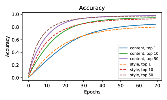
Figure 14: Accuracy and loss after training a linear classifier to predict the celebrity’s identity. Note that there are 10,177 identities in total, which makes this task hard, so we also show top-10 and top-50 accuracies.

We test our model on CelebA, which is a more challenging dataset. The dataset contains pictures of celebrities, where each image is assigned a subset of attributes among 40 possible attributes. Thus, we create 40 clients, give a unique attribute to each, and then show them the subset with this attribute. Note that this is not a partition, as some data will be repeated many times, but we want to see if the client will learn a biased style towards the assigned attributes.

To make the simulation feasible, we create 10 workers with their models, each handling a unique subset of 4 clients, and let each worker sample their clients in a round-robin fashion. Thus, each worker will always see at least one of 4 attributes. We train our model for approximately 200 communication rounds, with 2 epochs per round and train the discriminators 5 times as frequently as the generator (i.e. $T_{D}=5$).

Given some content latent, we can see that the client-specific attributes become more obvious in some clients than others. For example, lipsticks, moustaches, blonde hair, and other attributes are clearer in some clients than in others. See Figs. 15, 16 and 17 for samples from each worker.

For completeness and a better understanding of the generation quality, we list the attributes assigned to each worker:

1. Worker 1: [’Mustache’, ’Mouth_Slightly_Open’, ’Sideburns’, ’Big_Lips’].

2. Worker 2: [’Attractive’, ’Narrow_Eyes’, ’Gray_Hair’, ’Bald’].

3. Worker 3: [’Arched_Eyebrows’, ’Bangs’, ’Chubby’, ’Eyeglasses’].

4. Worker 4: [’Male’, ’Rosy_Cheeks’, ’Wearing_Necktie’, ’High_Cheekbones’].

5. Worker 5: [’Straight_Hair’, ’Wearing_Earrings’, ’Black_Hair’, ’No_Beard’].

6. Worker 6: [’5_o_Clock_Shadow’, ’Young’, ’Wearing_Necklace’, ’Wavy_Hair’].

7. Worker 7: [’Receding_Hairline’, ’Bushy_Eyebrows’, ’Goatee’, ’Heavy_Makeup’].

8. Worker 8: [’Pointy_Nose’, ’Blond_Hair’, ’Double_Chin’, ’Oval_Face’].

9. Worker 9: [’Big_Nose’, ’Smiling’, ’Blurry’, ’Brown_Hair’].

10. Worker 10: [’Wearing_Lipstick’, ’Pale_Skin’, ’Bags_Under_Eyes’, ’Wearing_Hat’].

Celebrity identification from representation. We also test the content and style features on a celebrity-identification task. The construction of the dataset is done so that we only test whether the style introduces a bias towards some attributes given some content, so we do not expect to see disentanglement between content and style. If we see one and only one attribute per client, then we might expect an attribute to be a style in the sense that it constitutes a domain, as in our MNIST example. In Fig. 14, we show the accuracy of a linear classifier on the content and style representations. Both achieve decent top-1 accuracies (84% and 79%, resp.), good 90% in top-10 accuracies (95% and 93%, resp.). Note that using top-10 and top-50 is approximately within the same proportion as using top-1 and top-5 for ImageNet, which has 1000 classes.

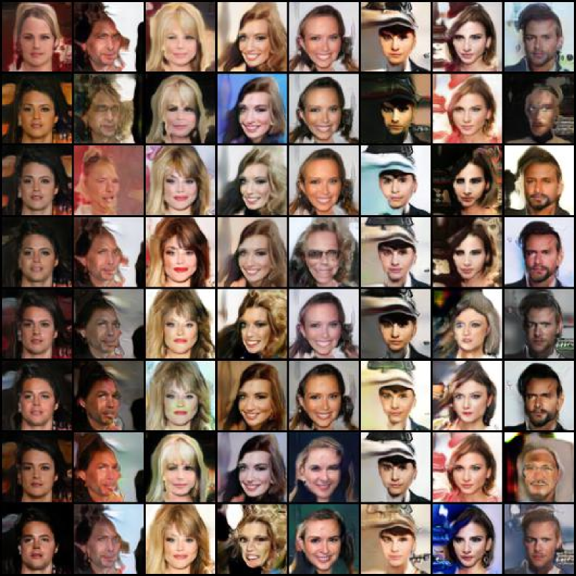
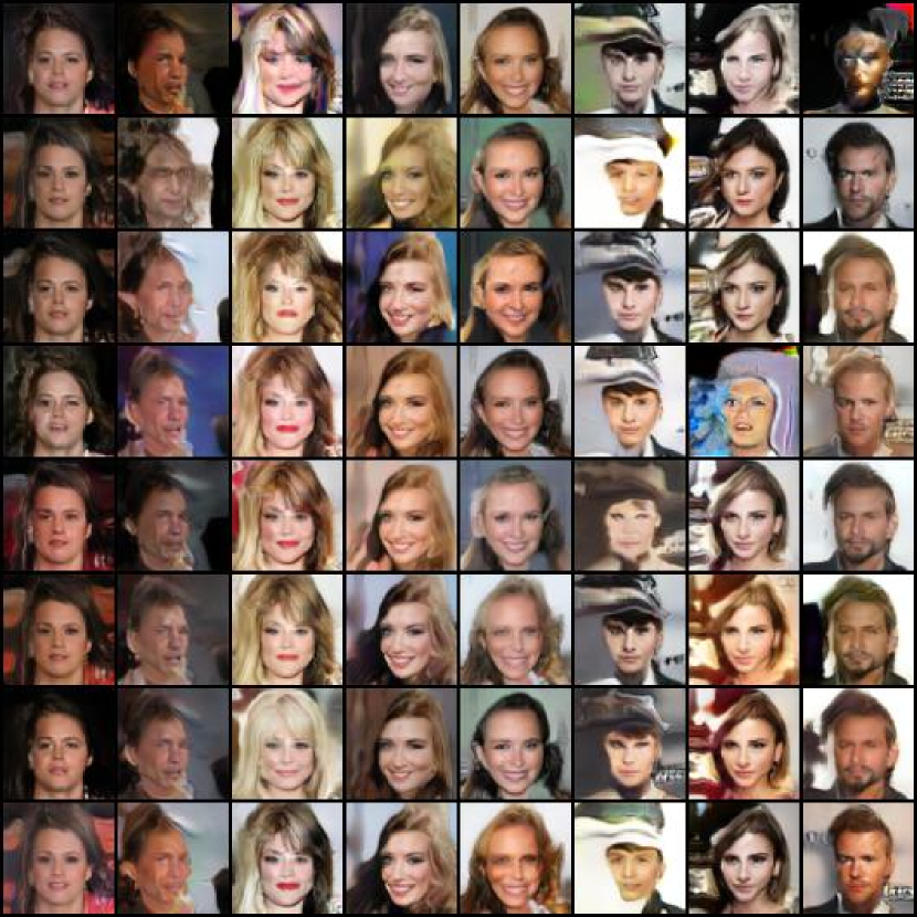
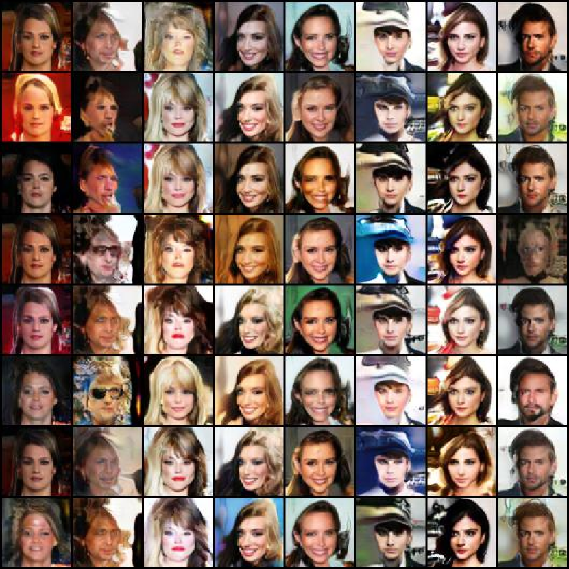
(a) Changing $\mathbf{z}^{s}$ per row while fixing $\mathbf{z}^{c}$.

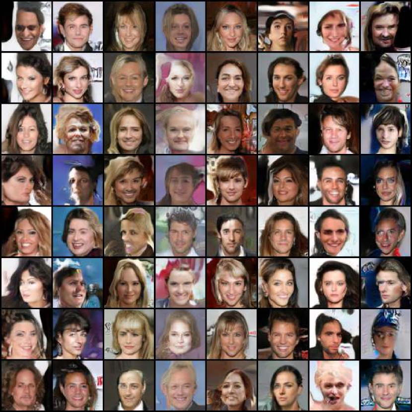
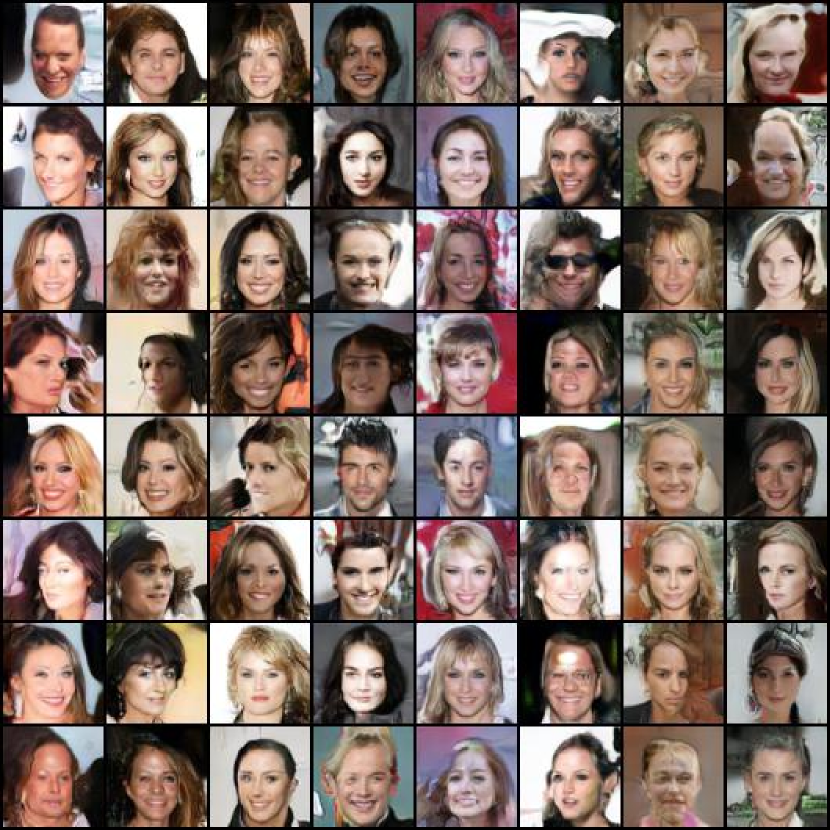
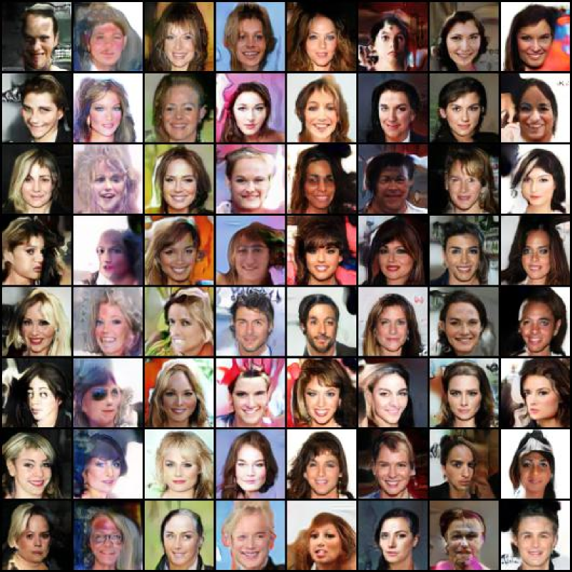
(b) Changing $\mathbf{z}^{c}$ per row while fixing $\mathbf{z}^{s}$.

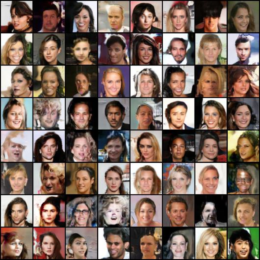
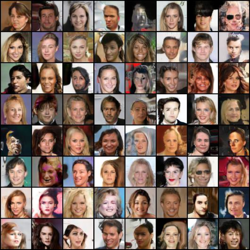
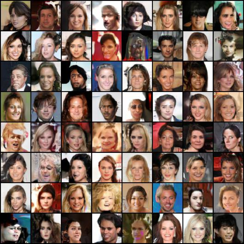
(c) Changing both $\mathbf{z}^{c}$ and $\mathbf{z}^{s}$.

Figure 15: Workers 1 at the top, 2 in the middle, and 3 at the bottom.

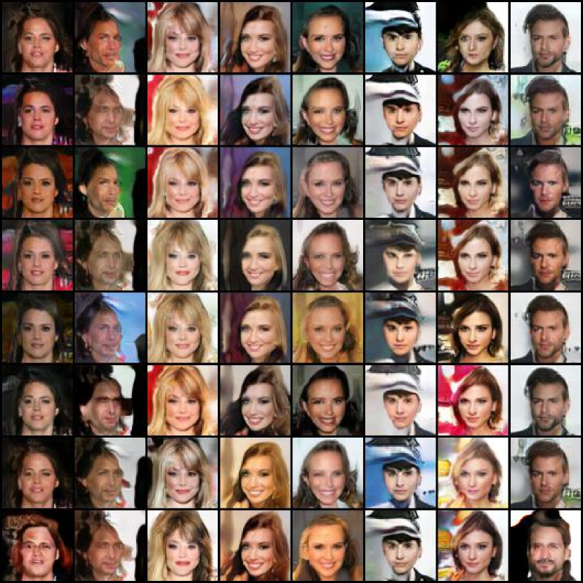
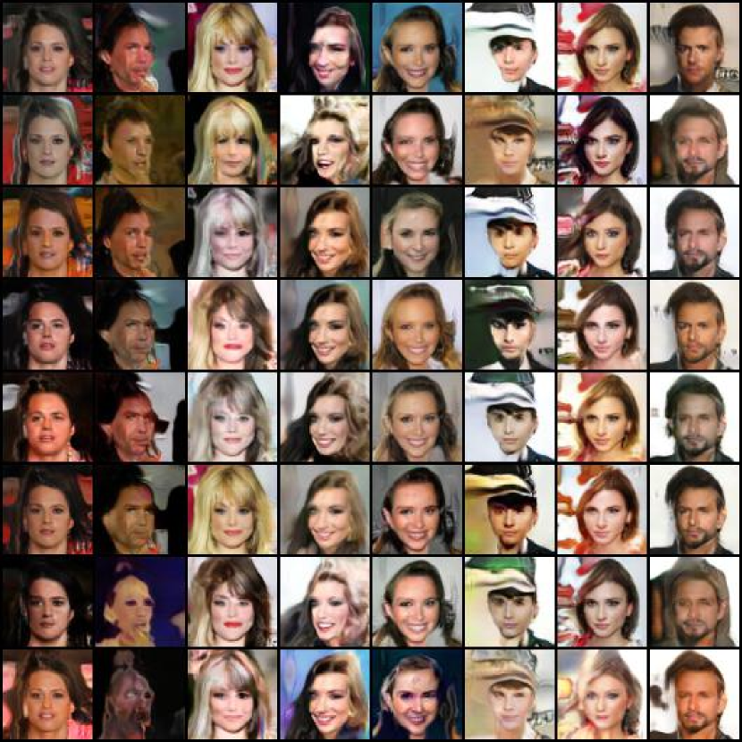
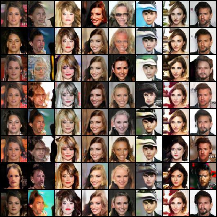
(a) Changing $\mathbf{z}^{s}$ per row while fixing $\mathbf{z}^{c}$.

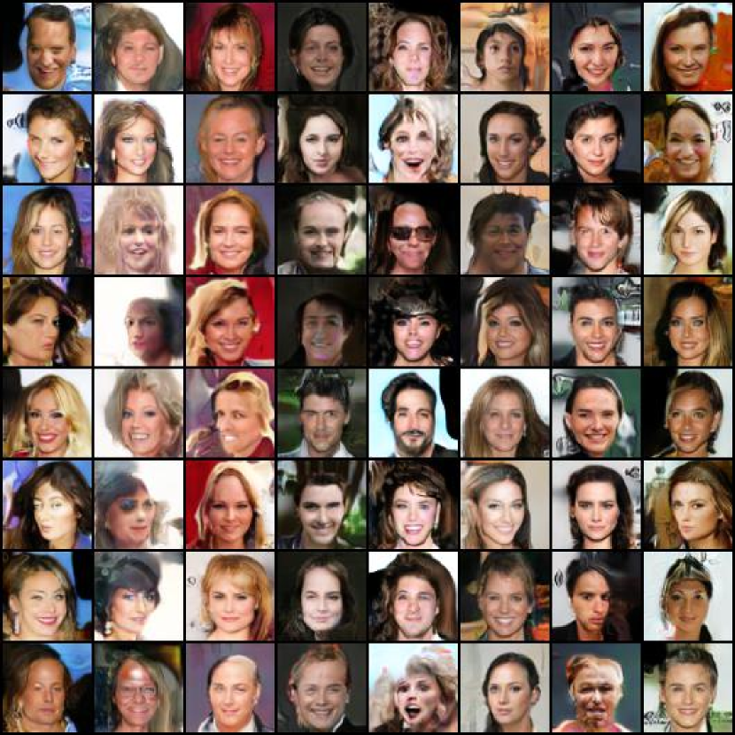
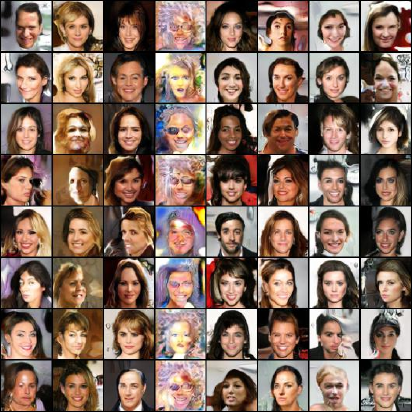
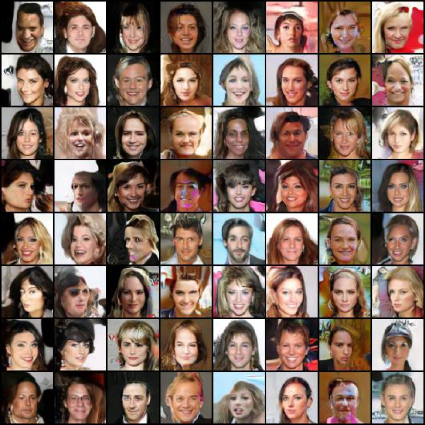
(b) Changing $\mathbf{z}^{c}$ per row while fixing $\mathbf{z}^{s}$.

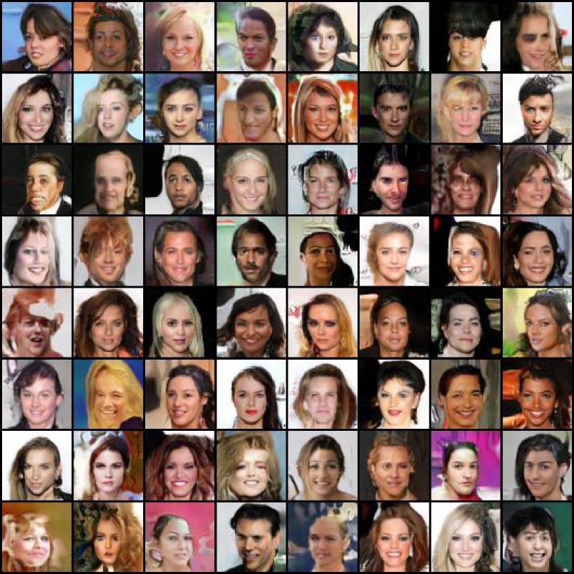
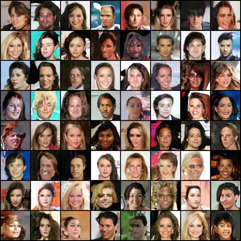
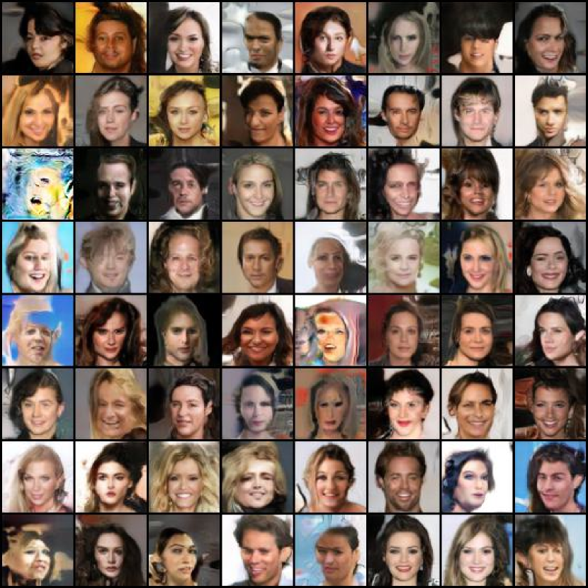
(c) Changing both $\mathbf{z}^{c}$ and $\mathbf{z}^{s}$.

Figure 16: Workers 4 at the top, 5 in the middle, and 6 at the bottom.

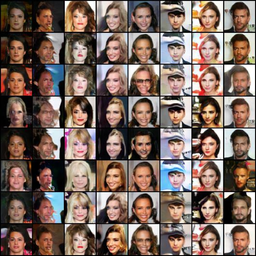
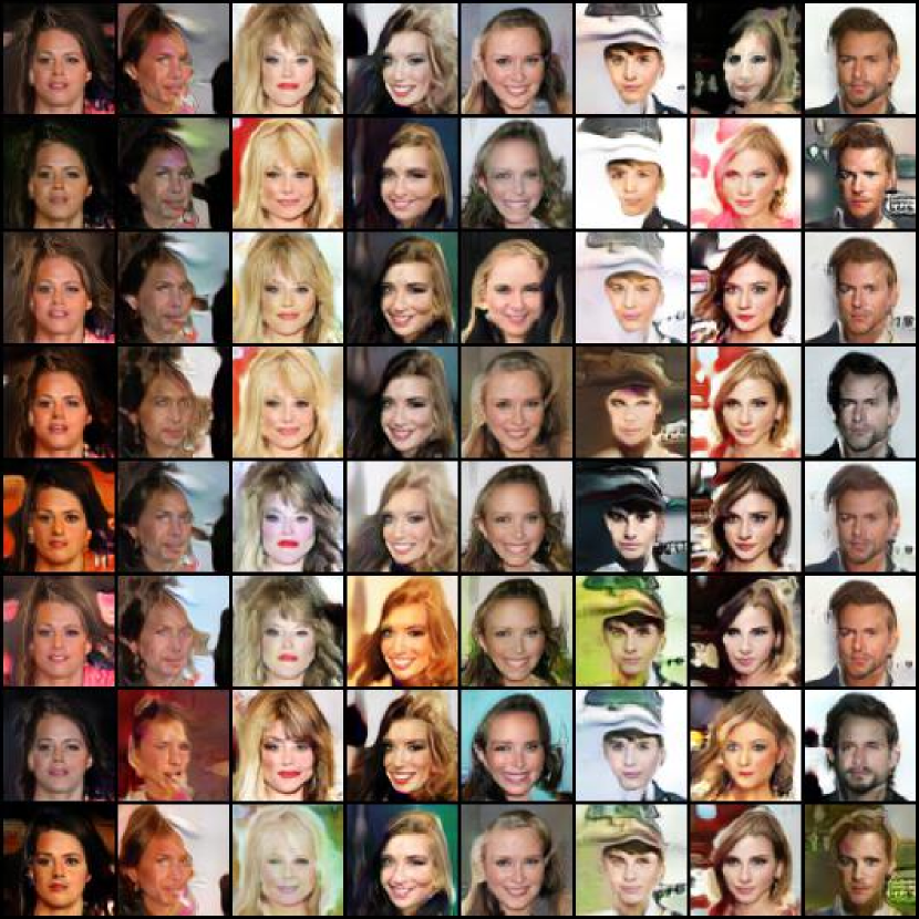
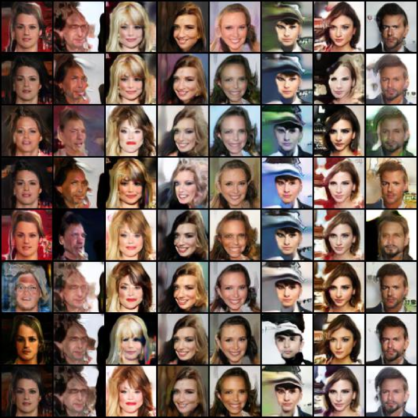
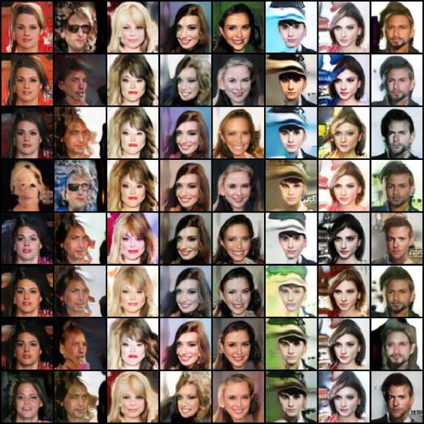
(a) Changing $\mathbf{z}^{s}$ per row while fixing $\mathbf{z}^{c}$.

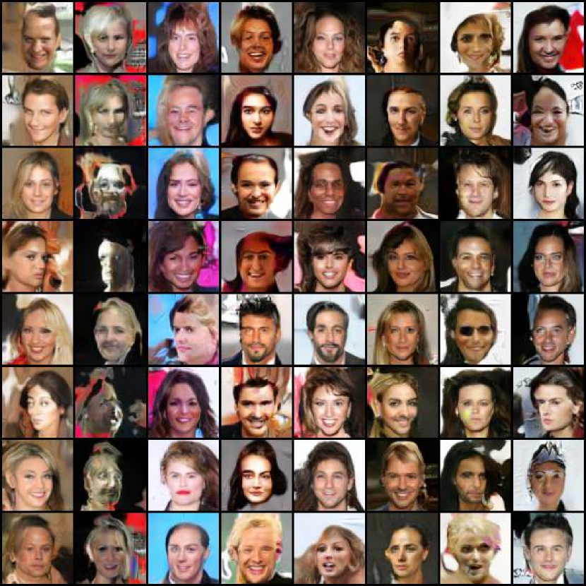
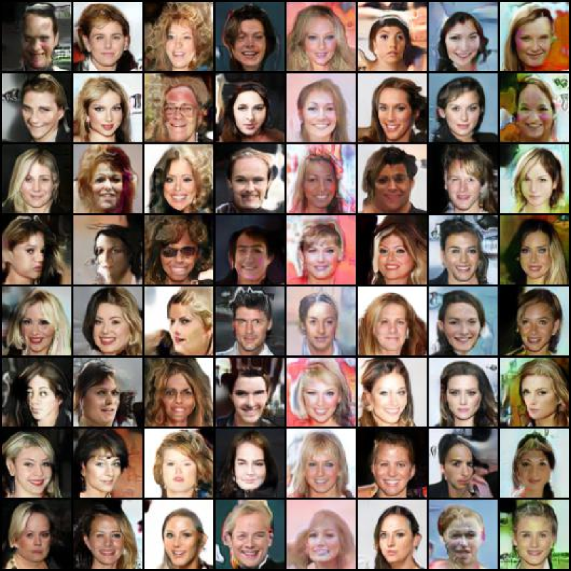
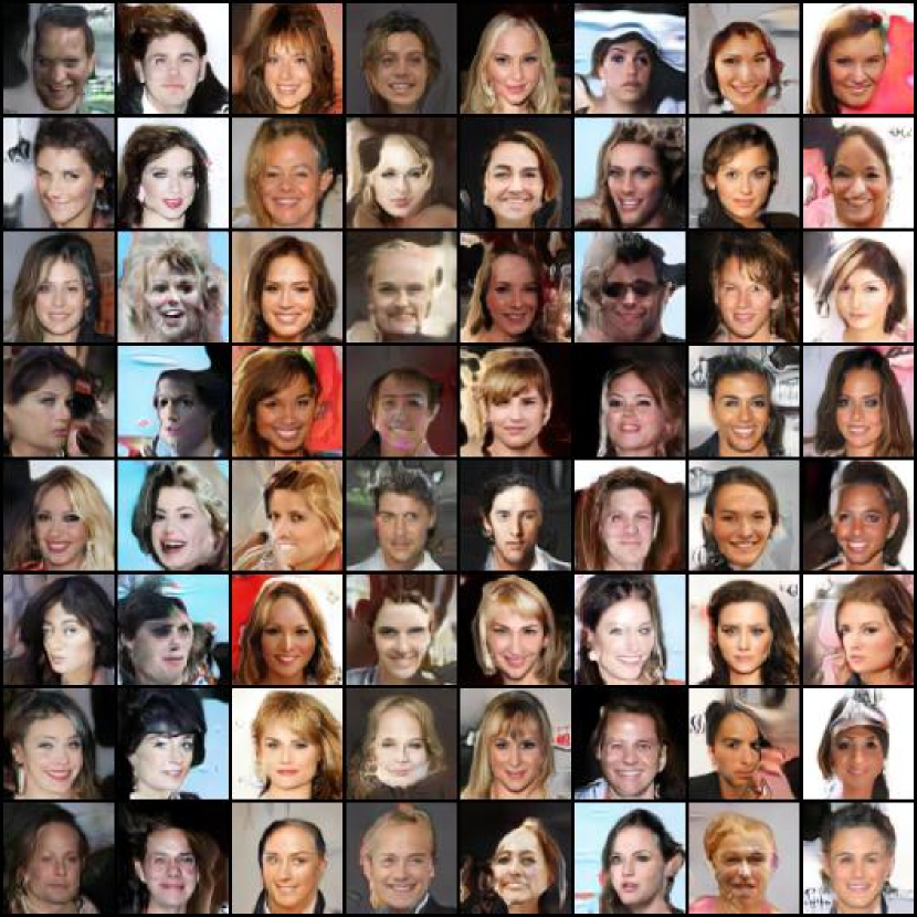
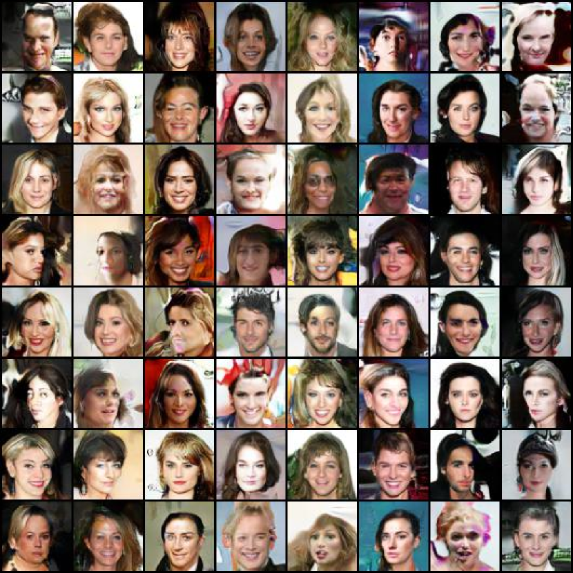
(b) Changing $\mathbf{z}^{c}$ per row while fixing $\mathbf{z}^{s}$.

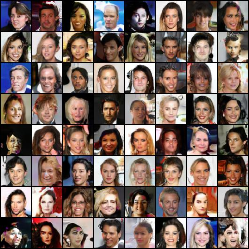
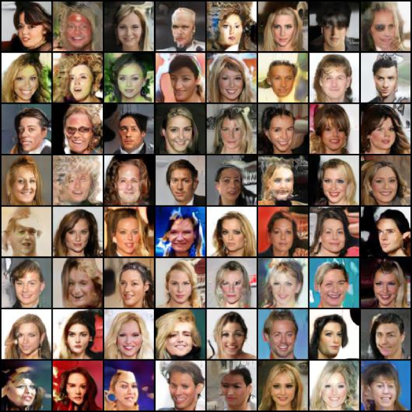
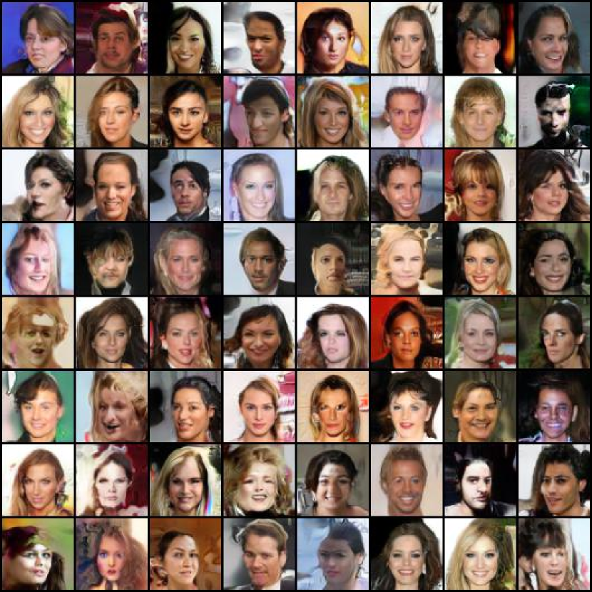
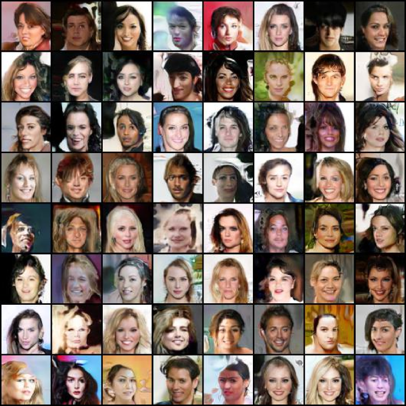
(c) Changing both $\mathbf{z}^{c}$ and $\mathbf{z}^{s}$.

Figure 17: Workers 7 at the top, 8 in the upper-middle, 9 in the lower-middle, and 10 at the bottom.

References

- [1] Manoj Ghuhan Arivazhagan, Vinay Aggarwal, Aaditya Kumar Singh, and Sunav Choudhary. Federated learning with personalization layers, 2019.
- [2] Sean Augenstein, H. Brendan McMahan, Daniel Ramage, Swaroop Ramaswamy, Peter Kairouz, Mingqing Chen, Rajiv Mathews, and Blaise Agüera y Arcas. Generative models for effective ML on private, decentralized datasets. In 8th International Conference on Learning Representations, ICLR 2020, Addis Ababa, Ethiopia, April 26-30, 2020. OpenReview.net, 2020.
- [3] Horace Barlow. Redundancy reduction revisited. Network: computation in neural systems, 12(3):241, 2001.
- [4] Duc Bui, Kshitiz Malik, Jack Goetz, Honglei Liu, Seungwhan Moon, Anuj Kumar, and Kang G Shin. Federated user representation learning. arXiv preprint arXiv:1909.12535, 2019.
- [5] Ting Chen, Simon Kornblith, Mohammad Norouzi, and Geoffrey Hinton. A simple framework for contrastive learning of visual representations. In International conference on machine learning, pages 1597–1607. PMLR, 2020.
- [6] Xinlei Chen and Kaiming He. Exploring simple siamese representation learning. In Proceedings of the IEEE/CVF Conference on Computer Vision and Pattern Recognition, pages 15750–15758, 2021.
- [7] Harm De Vries, Florian Strub, Jérémie Mary, Hugo Larochelle, Olivier Pietquin, and Aaron C Courville. Modulating early visual processing by language. Advances in Neural Information Processing Systems, 30, 2017.
- [8] Enmao Diao, Jie Ding, and Vahid Tarokh. Heterofl: Computation and communication efficient federated learning for heterogeneous clients. arXiv preprint arXiv:2010.01264, 2020.
- [9] Alexey Dosovitskiy, Lucas Beyer, Alexander Kolesnikov, Dirk Weissenborn, Xiaohua Zhai, Thomas Unterthiner, Mostafa Dehghani, Matthias Minderer, Georg Heigold, Sylvain Gelly, Jakob Uszkoreit, and Neil Houlsby. An image is worth 16x16 words: Transformers for image recognition at scale. In 9th International Conference on Learning Representations, ICLR 2021, Virtual Event, Austria, May 3-7, 2021. OpenReview.net, 2021.
- [10] Chenyou Fan and Ping Liu. Federated generative adversarial learning, 2020.
- [11] Ian Goodfellow, Jean Pouget-Abadie, Mehdi Mirza, Bing Xu, David Warde-Farley, Sherjil Ozair, Aaron Courville, and Yoshua Bengio. Generative adversarial networks. Communications of the ACM, 63(11):139–144, 2020.
- [12] Luigi Gresele, Julius Von Kügelgen, Vincent Stimper, Bernhard Schölkopf, and Michel Besserve. Independent mechanism analysis, a new concept? Advances in neural information processing systems, 34:28233–28248, 2021.
- [13] Ishaan Gulrajani, Faruk Ahmed, Martin Arjovsky, Vincent Dumoulin, and Aaron C Courville. Improved training of wasserstein gans. Advances in neural information processing systems, 30, 2017.
- [14] Kaiming He, Haoqi Fan, Yuxin Wu, Saining Xie, and Ross Girshick. Momentum contrast for unsupervised visual representation learning. In Proceedings of the IEEE/CVF conference on computer vision and pattern recognition, pages 9729–9738, 2020.
- [15] Kaiming He, Xiangyu Zhang, Shaoqing Ren, and Jian Sun. Deep residual learning for image recognition. In Proceedings of the IEEE conference on computer vision and pattern recognition, pages 770–778, 2016.
- [16] Jonathan Ho, Ajay Jain, and Pieter Abbeel. Denoising diffusion probabilistic models. Advances in Neural Information Processing Systems, 33:6840–6851, 2020.
- [17] Samuel Horváth, Stefanos Laskaridis, Mario Almeida, Ilias Leontiadis, Stylianos Venieris, and Nicholas Lane. Fjord: Fair and accurate federated learning under heterogeneous targets with ordered dropout. In M. Ranzato, A. Beygelzimer, Y. Dauphin, P.S. Liang, and J. Wortman Vaughan, editors, Advances in Neural Information Processing Systems, volume 34, pages 12876–12889. Curran Associates, Inc., 2021.
- [18] Jongheon Jeong and Jinwoo Shin. Training gans with stronger augmentations via contrastive discriminator. arXiv preprint arXiv:2103.09742, 2021.
- [19] Peter Kairouz, H. Brendan McMahan, Brendan Avent, Aurélien Bellet, Mehdi Bennis, Arjun Nitin Bhagoji, Kallista Bonawitz, Zachary Charles, Graham Cormode, Rachel Cummings, Rafael G. L. D’Oliveira, Hubert Eichner, Salim El Rouayheb, David Evans, Josh Gardner, Zachary Garrett, Adrià Gascón, Badih Ghazi, Phillip B. Gibbons, Marco Gruteser, Zaid Harchaoui, Chaoyang He, Lie He, Zhouyuan Huo, Ben Hutchinson, Justin Hsu, Martin Jaggi, Tara Javidi, Gauri Joshi, Mikhail Khodak, Jakub Konečný, Aleksandra Korolova, Farinaz Koushanfar, Sanmi Koyejo, Tancrède Lepoint, Yang Liu, Prateek Mittal, Mehryar Mohri, Richard Nock, Ayfer Özgür, Rasmus Pagh, Mariana Raykova, Hang Qi, Daniel Ramage, Ramesh Raskar, Dawn Song, Weikang Song, Sebastian U. Stich, Ziteng Sun, Ananda Theertha Suresh, Florian Tramèr, Praneeth Vepakomma, Jianyu Wang, Li Xiong, Zheng Xu, Qiang Yang, Felix X. Yu, Han Yu, and Sen Zhao. Advances and open problems in federated learning, 2019.
- [20] Minguk Kang and Jaesik Park. Contragan: Contrastive learning for conditional image generation. In H. Larochelle, M. Ranzato, R. Hadsell, M.F. Balcan, and H. Lin, editors, Advances in Neural Information Processing Systems, volume 33, pages 21357–21369. Curran Associates, Inc., 2020.
- [21] Tero Karras, Samuli Laine, and Timo Aila. A style-based generator architecture for generative adversarial networks. In Proceedings of the IEEE/CVF conference on computer vision and pattern recognition, pages 4401–4410, 2019.
- [22] Diederik P Kingma and Jimmy Ba. Adam: A method for stochastic optimization. arXiv preprint arXiv:1412.6980, 2014.
- [23] Diederik P Kingma and Max Welling. Auto-encoding variational bayes. arXiv preprint arXiv:1312.6114, 2013.
- [24] Jakub Konečný, H. Brendan McMahan, Daniel Ramage, and Peter Richtárik. Federated optimization: Distributed machine learning for on-device intelligence, 2016.
- [25] Jakub Konečný, H. Brendan McMahan, Felix X. Yu, Peter Richtárik, Ananda Theertha Suresh, and Dave Bacon. Federated learning: Strategies for improving communication efficiency, 2016.
- [26] Lingjing Kong, Shaoan Xie, Weiran Yao, Yujia Zheng, Guangyi Chen, Petar Stojanov, Victor Akinwande, and Kun Zhang. Partial disentanglement for domain adaptation. In Kamalika Chaudhuri, Stefanie Jegelka, Le Song, Csaba Szepesvari, Gang Niu, and Sivan Sabato, editors, Proceedings of the 39th International Conference on Machine Learning, volume 162 of Proceedings of Machine Learning Research, pages 11455–11472. PMLR, 17–23 Jul 2022.
- [27] Phuc H. Le-Khac, Graham Healy, and Alan F. Smeaton. Contrastive representation learning: A framework and review. IEEE Access, 8:193907–193934, 2020.
- [28] Yann LeCun, Léon Bottou, Yoshua Bengio, and Patrick Haffner. Gradient-based learning applied to document recognition. Proceedings of the IEEE, 86(11):2278–2324, 1998.
- [29] Tian Li, Anit Kumar Sahu, Manzil Zaheer, Maziar Sanjabi, Ameet Talwalkar, and Virginia Smith. Federated optimization in heterogeneous networks, 2018.
- [30] Kuo-Yun Liang, Abhishek Srinivasan, and Juan Carlos Andresen. Modular federated learning. In 2022 International Joint Conference on Neural Networks (IJCNN). IEEE, jul 2022.
- [31] Xiao Liu, Fanjin Zhang, Zhenyu Hou, Li Mian, Zhaoyu Wang, Jing Zhang, and Jie Tang. Self-supervised learning: Generative or contrastive. IEEE Transactions on Knowledge and Data Engineering, 2021.
- [32] Ziwei Liu, Ping Luo, Xiaogang Wang, and Xiaoou Tang. Deep learning face attributes in the wild. In Proceedings of International Conference on Computer Vision (ICCV), December 2015.
- [33] H. Brendan McMahan, Eider Moore, Daniel Ramage, Seth Hampson, and Blaise Agüera y Arcas. Communication-efficient learning of deep networks from decentralized data. 2016.
- [34] Takeru Miyato, Toshiki Kataoka, Masanori Koyama, and Yuichi Yoshida. Spectral normalization for generative adversarial networks. In 6th International Conference on Learning Representations, ICLR 2018, Vancouver, BC, Canada, April 30 - May 3, 2018, Conference Track Proceedings. OpenReview.net, 2018.
- [35] Takeru Miyato and Masanori Koyama. cgans with projection discriminator. In 6th International Conference on Learning Representations, ICLR 2018, Vancouver, BC, Canada, April 30 - May 3, 2018, Conference Track Proceedings. OpenReview.net, 2018.
- [36] Aaron van den Oord, Yazhe Li, and Oriol Vinyals. Representation learning with contrastive predictive coding. arXiv preprint arXiv:1807.03748, 2018.
- [37] Judea Pearl. Causality. Cambridge university press, 2009.
- [38] Krishna Pillutla, Kshitiz Malik, Abdel-Rahman Mohamed, Mike Rabbat, Maziar Sanjabi, and Lin Xiao. Federated learning with partial model personalization. In Kamalika Chaudhuri, Stefanie Jegelka, Le Song, Csaba Szepesvari, Gang Niu, and Sivan Sabato, editors, Proceedings of the 39th International Conference on Machine Learning, volume 162 of Proceedings of Machine Learning Research, pages 17716–17758. PMLR, 17–23 Jul 2022.
- [39] Mohammad Rasouli, Tao Sun, and Ram Rajagopal. Fedgan: Federated generative adversarial networks for distributed data, 2020.
- [40] Bernhard Schölkopf, Francesco Locatello, Stefan Bauer, Nan Rosemary Ke, Nal Kalchbrenner, Anirudh Goyal, and Yoshua Bengio. Toward causal representation learning. Proceedings of the IEEE, 109(5):612–634, 2021.
- [41] Karan Singhal, Hakim Sidahmed, Zachary Garrett, Shanshan Wu, John Rush, and Sushant Prakash. Federated reconstruction: Partially local federated learning. Advances in Neural Information Processing Systems, 34:11220–11232, 2021.
- [42] Ashish Vaswani, Noam Shazeer, Niki Parmar, Jakob Uszkoreit, Llion Jones, Aidan N Gomez, Łukasz Kaiser, and Illia Polosukhin. Attention is all you need. Advances in neural information processing systems, 30, 2017.
- [43] Praneeth Vepakomma, Otkrist Gupta, Tristan Swedish, and Ramesh Raskar. Split learning for health: Distributed deep learning without sharing raw patient data. arXiv preprint arXiv:1812.00564, 2018.
- [44] Jianyu Wang, Zachary Charles, Zheng Xu, Gauri Joshi, H. Brendan McMahan, Blaise Aguera y Arcas, Maruan Al-Shedivat, Galen Andrew, Salman Avestimehr, Katharine Daly, Deepesh Data, Suhas Diggavi, Hubert Eichner, Advait Gadhikar, Zachary Garrett, Antonious M. Girgis, Filip Hanzely, Andrew Hard, Chaoyang He, Samuel Horvath, Zhouyuan Huo, Alex Ingerman, Martin Jaggi, Tara Javidi, Peter Kairouz, Satyen Kale, Sai Praneeth Karimireddy, Jakub Konecny, Sanmi Koyejo, Tian Li, Luyang Liu, Mehryar Mohri, Hang Qi, Sashank J. Reddi, Peter Richtarik, Karan Singhal, Virginia Smith, Mahdi Soltanolkotabi, Weikang Song, Ananda Theertha Suresh, Sebastian U. Stich, Ameet Talwalkar, Hongyi Wang, Blake Woodworth, Shanshan Wu, Felix X. Yu, Honglin Yuan, Manzil Zaheer, Mi Zhang, Tong Zhang, Chunxiang Zheng, Chen Zhu, and Wennan Zhu. A field guide to federated optimization, 2021.
- [45] Yixin Wang and Michael I Jordan. Desiderata for representation learning: A causal perspective. arXiv preprint arXiv:2109.03795, 2021.
- [46] Ryo Yonetani, Tomohiro Takahashi, Atsushi Hashimoto, and Yoshitaka Ushiku. Decentralized learning of generative adversarial networks from non-iid data, 2019.
- [47] Ning Yu, Guilin Liu, Aysegul Dundar, Andrew Tao, Bryan Catanzaro, Larry S Davis, and Mario Fritz. Dual contrastive loss and attention for gans. In Proceedings of the IEEE/CVF International Conference on Computer Vision, pages 6731–6742, 2021.
- [48] Jure Zbontar, Li Jing, Ishan Misra, Yann LeCun, and Stéphane Deny. Barlow twins: Self-supervised learning via redundancy reduction. In International Conference on Machine Learning, pages 12310–12320. PMLR, 2021.
- [49] Kun Zhang, Bernhard Schölkopf, Krikamol Muandet, and Zhikun Wang. Domain adaptation under target and conditional shift. In International conference on machine learning, pages 819–827. PMLR, 2013.
- [50] Roland S. Zimmermann, Yash Sharma, Steffen Schneider, Matthias Bethge, and Wieland Brendel. Contrastive learning inverts the data generating process. 139:12979–12990, 2021.