The Branch-cut Cosmology: A topological canonical quantum approach

Abstract

In this contribution we sketch a branch-cut quantum formulation of the Wheeler-DeWitt equation analytically continued to the complex plane. As a starting point, we base our approach on the Hořava-Lifshitz formulation of gravity, which employs higher spatial-derivative terms of the spacetime curvature for renormalisation reasons. Following standard procedures, the quantization of the Lagrangian density is achieved by raising the Hamiltonian, the dynamical variable $\ln^{-1}[\beta(t)]$, which represents the the branch-cut complex scale factor, and the conjugate momentum $p_{\rm{\ln}}$ to the category of operators. We arrive at an Schrodinger-type equation with a non-linear potential. Solutions are then obtained and discussed for different potential parameterizations. The results reinforce the conception of a quantum leap between the contraction and expansion phases of the branch-cut universe, in good agreement with the Bekenstein criterion.

1 Introduction

The consistent reconciliation of general relativity (GR) and quantum mechanics(QM) presents inherent mathematical and conceptual difficulties. The main problem lies in the fact that relativity and quantum mechanics are fundamentally different theories, generating at different scales formal incompatibilities between two genuinely consistent descriptions of reality.

On the Planck scale, general relativity, based on the geometric properties of a smooth unified spacetime manifold, and quantum mechanics, a probabilistic formulation where time corresponds to an universal and absolute parameter, are supposed to merge into an unified theory of quantum gravity.

General relativity provides meaningless answers when reduced to quantum dimensions. Quantum mechanics, on the other hand, lacks conceptual and formal consistency when expanded to cosmic dimensions.

Furthermore, general relativity describes continuous and deterministic events, reducing causes and effects to a specific location. In quantum mechanics in turn, events produced by the interactions between elementary particles happen in quantum leaps, whose results are probabilistic rather than deterministic. Moreover, in quantum mechanics laws and rules admit connections prohibited by classical physics.

The formal treatment of time in quantum mechanics also differs from that given in general relativity. In quantum mechanics, due to its absolute and universal character, the treatment given to time differs from the treatment given to the other coordinates that unlike time can be elevated to the category of quantum operators and observables. since in QM the time coordinate plays an essentially different role from the position coordinates: while position is represented by a Hermitian operator, time is represented by a c-number.

In general relativity, unlike Newtonian physics and quantum mechanics, where the variable time $t$ represents the ‘reading of a clock’, this reading is not given by $t$ but instead by

$$T=\int_{\gamma}\sqrt{g_{\mu\nu}(\vec{x},t)dx^{\mu}dx^{\nu}}\,,$$ (1)

which defines a line integral depending on the gravitational field, $g_{\mu\nu}(\vec{x},t)$, computed along the clock’s worldline $\gamma$ (Rovelli, 2015). The coordinate $t$ in the argument of $g_{\mu\nu}(\vec{x},t)$ despite representing the evolution parameter of the Lagrangian and Hamiltonian formalism, in general relativity has no direct physical meaning, and according to Rovelli (2015), “can be changed freely”.

The description of Rovelli (2015) about the role of the variable $t$ in general relativity is very illuminating. Suppose the readings of two clocks, $T_{1}$ and $T_{2}$ as given in Equation 1. General relativity then describes the relative evolution of these variables computed along different worldliness, with respect to one another, assumed to be on the same level of equality and do not consider the absolute evolution of any of those variables in time.

From a mathematical point of view, an adequate representation of this relative evolution would be $T_{1}(T_{2})$ and $T_{2}(T_{1})$. However, for simplicity and broad description what general relativity does is replace the arguments of these representations with an arbitrary parameter, $t$, and use the parametric form of representation $T_{1}(t)$ and $T_{2}(t)$, where the variable $t$ can be chosen freely. In these examples, $t$ is the same parameter that appears in the definition of the gravitational field in Equation 1. So, general relativity describes the relative evolution of variable quantities with respect to one another instead of the exclusive absolute evolution of any of these variables in time (see Rovelli (2019) for more details).

In the following we propose a topological canonical quantum approach for the branch-cut cosmology (Zen Vasconcellos ., 2020, 20212, 20211, 2022) based on the geometrodynamics Wheeler-DeWitt equation (DeWitt, 1967), based upon canonical quantization of constrained systems (TP. Shestakova, 2018). The solution of the WDW equation, the wave function of the universe, is thus a functional on the geometries of compact three-manifolds and on the values of the matter fields on these manifolds and describes the quantum states of a spatially closed universe (Hartle  Hawking, 1983). As a corollary, our expectations concerning this approach are that the Wheeler DeWitt equation, “properly understood and properly defined”, may give the “full dynamics of quantum gravity” Rovelli (2015).

Despite the wide range of meanings of this statement, in the present work, by proposing a quantum formulation of branch-cut cosmology, in this approach we limit ourselves, for a comparison with formulations based on the standard model, to a formulation with a real potential, however extending the formulation to a conjugate representation of the original representation. We thus fulfill one of the most striking conclusions of branch-cut cosmology.

2 The Weeler and DeWitt Equation

On basis of the audacious idea of physics without time as the direct outcome of conversations with Wheeler DeWitt (1967) introduced a canonical formulation of quantum gravity, known today as the Wheeler DeWitt equation.

Despite the uncertainties involving the original formulation, the main one related to time suppression (see Rovelli (2015)), the WDW equation is considered a milestone in the development of quantum gravity. At present, the absence of time in this equation is perfectly understandable and consistent with current interpretations of the role of time in general relativity.

The Wheeler-DeWitt formulation for quantum gravity consists in constraining a wave-function which applies to the universe as a whole, the so called wave function of the universe, in accordance with the Dirac recipe:

$$\hat{\cal H}\Psi=0\,,$$ (2)

i.e., a stationary, timeless equation, instead of a time-dependent quantum mechanics wave equation as for instance

$$i\frac{\partial}{\partial t}\Psi=\hat{H}\Psi\,.$$ (3)

Here, $\hat{H}$ denotes the Hamiltonian operator of a quantum subsystem, while $\hat{\cal H}$ in the previous equation represents a quantum operator which describes a general relativity constraint, resulting in a second order hyperbolic equation of gravity variables. The WDW equations thus constitutes a Klein-Gordon-type equation, having therefore a ‘natural’ conserved associated current (${\cal J}$),

$${\cal J}=\frac{i}{2}\Bigl{(}\Psi^{\dagger}\,\nabla\cdot\Psi-\Psi\,\nabla\cdot\Psi^{\dagger}\Bigr{)};\,\,\,\mbox{with}\,\,\nabla\cdot{\cal J}=0\,.$$ (4)

The Wheeler-DeWitt equation presents some notable features that are distinguishable from the Schrödinger equation. The main feature, as stressed before, is the absence of the time coordinate such that the ‘universe wave-function $\Psi$’ depends only on the three-dimensional spatial coordinates, giving rise to the well-known ‘time problem’ (Rovelli  Smerlak, 2011; Rovelli, 2015).

The main reason for the absence of a specific external coordinate of time lies in the covariance imposition of general relativity, more precisely, the wave function is only a function of the “3-geometry”, due namely to the equivalence class of metrics under a diffeomorphism (for the details see Rovelli (2015)). The second important feature is that the original version of the WDW wave equation is real instead of complex. This characteristic is due to the intrinsic union between the time variable and the imaginary unit $i$ in the definition of space-time. Evidently, in what follows, in view of the complexification of the FLRW metric in the branch-cut cosmology, the corresponding WDW-type equation presents different conceptual components with respect to both the meaning of the wave function of the universe, as well as the understanding of the corresponding continuity equation, among others.

Based on this understanding, in the following we sketch a branch-cut quantum formulation of the WDW equation analytically continued to the complex plane, characterized by only one dynamical variable, the branch-cut complex scale factor $\ln^{-1}[\beta(t)]$ (see (Zen Vasconcellos ., 2020, 20212, 20211)).

3 Hořava-Lifshitz action

The Hořava-Lifshitz formulation of gravity (Hořava, 2009; Cordero ., 2019; García-Compeán  Mata-Pacheco, 2022; Garattini  Faizal, 2016; Vakili  Kord, 2013; Chojnacki  Kwapisz, 2021) is an alternative theory to general relativity which employs higher spatial-derivative terms of the spacetime curvature which are added to the Einstein- Hilbert action with the aim of obtaining a renormalisable theory. The Hořava-Lifshitz (HL) gravity model preserves high and low energy scales and proposes the ultraviolet completion and a power-countable renormalization of gravity at the UV fixed point, additionally recovering the standard theory at the fixed infrared point, as well as Lorentz symmetry. Hořava–Lifshitz topological gravity addresses, in its original formulation, quantum mechanics as the fundamental theoretical framework so that space and time are not equivalent and therefore anisotropic.

In the following, as a simplification, instead of adopting a superspace formulation we assume as a starting point a homogeneous and isotropic multiverse restricted to a mini-superspace (see for instance (Kim, 1997)), corresponding to a 4-dimensional space-time branch-cut universe manifold, $\cal{M}$, decomposed into $3+1$ dimensions.

The branch-cut cosmology is characterized by only one dynamical variable, the branch-cut complex scale factor $\ln^{-1}[\beta(t)]$. The branch-cut manifold $\cal{M}$ is foliated into hypersurfaces, $\Sigma_{t}$, constricted to Riemann sheets labeled by a complex parameter of time, $t$, with the 4-dimensional analytically continued branch-cut line element given as (Zen Vasconcellos ., 20212, 20211)

$$ds_{[\rm{ac}]}^{2}=-\sigma^{2}N^{2}(t)c^{2}dt^{2}+\sigma^{2}\ln^{-2}[\beta(t)]d\Omega^{2}(r,\theta,\phi)\,;$$ (5)

the metric of the unit 3-sphere is

$$d\Omega^{2}(r,\theta,\phi)\equiv\Biggl{[}\frac{dr^{2}}{\bigl{(}1-kr^{2}(t)\bigr{)}}+r^{2}(t)\Bigl{(}d\theta^{2}+sin^{2}\theta d\phi^{2}\Bigr{)}\Biggr{]}\,.$$ (6)

In this expression, the function $\beta(t)$ characterizes the range of $\ln^{-1}[\beta(t)]$ associated to the cuts in the branch-cut. The branch-cut complex scale factor $\ln^{-1}[\beta(t)]$ denotes solutions of Einstein’s equations for a FLRW-type metric extended to the complex plane, represented as the reciprocal of a complex multi-valued function, the natural complex logarithm function $\ln[\beta(t)]$, not its inverse. Moreover, in these expressions, $r$ and $t$ represent respectively real-space and complex-time parameters and $k$ encodes the spatial curvature of the multi-composed universe, $k=-1,0,1$ for, respectively, negatively curved, flat or positively curved spatial hyper-surfaces analytically continued to the complex plane.

In expression (5), $N(t)$ is an arbitrary lapse function and $\sigma^{2}=2/3\pi$ is just a normalisation factor. The lapse function $N(t)$ is not a dynamical quantity, but a pure gauge variable. Gauge invariance of the action in general relativity yields a Hamiltonian constraint which requires a gauge fixing condition on the lapse $N(t)$ (see Feinberg  Peleg (1995). The lapse function may be fully determined by the difference between the elapsed time-parameter $t$, and the proper time-parameter $\tau=N(t)dt$ on curves normal to a given hypersurface $\Sigma_{t}$ (Flinn, 2020; Wiltshire, 1996). A canonical analysis shows that the lapse function $N(t)$ and the ADM (Arnowitt ., 2004) shift vector $N^{i}(t)$ play the role of Lagrange multipliers (Kim, 1997). In the special case in which $N^{i}=0$, the spatial coordinates are said to be “comoving”. The shift vector $N_{i}$ describes how a given hyper-surface $\Sigma_{t}$ differs from a neighbouring hyper-surface $\Sigma_{t+dt}$. In this case the time-parameter component of the line element would be shifted to $N^{2}(t)\to N^{i}N_{i}$.

The extrinsic curvature is a symmetric, purely spatial mathematical construct that measures the geometrical changes and deformation rates of the normal to a hyper-surface as it is transported from one point to another. Extrinsic curvature corresponds to a manifold (actually a sub-manifold) which depends on its particular embedding. The extrinsic curvature tensor $K_{ij}$ can be written in terms of the three-metric in the following form (Bertolami  Zarro, 2011):

$$K_{ij}=\frac{1}{2\sigma N}\Biggl{(}-\frac{\partial g_{ij}}{\partial t}+\nabla_{i}N_{j}+\nabla_{j}N_{i}\Biggr{)}\,,$$ (7)

where $N^{i}$ $\nabla_{i}$ denotes the 3-dimensional covariant derivative, and $g_{ij}=\ln^{-1}[\beta(t)]diag\bigl{(}\frac{1}{1-r^{2}},r^{2},r^{2}sin^{2}\theta\bigr{)}$.

Since $N_{i}=0$ for RW-like spaces, corresponding to co-moving coordinates, the curvature tensor takes the form

$$K_{ij}=-\frac{1}{2\sigma N}\frac{\frac{d}{dt}\ln^{-1}[\beta(t)]}{\ln^{-1}[\beta(t)]}g_{ij}\,.$$ (8)

Taking the trace of the curvature tensor we get

$$K=K^{ij}g_{ij}=-\frac{3}{2\sigma N}\frac{\frac{d}{dt}\ln^{-1}[\beta(t)]}{\ln^{-1}[\beta(t)]}.$$ (9)

The next step is to write the Hořava-Lifshitz formulation of the Einstein–Hilbert action as a functional formulation of the spacetime metric $g_{\mu\nu}$. The dynamics of the system corresponds to a succession of three-dimensional space-like hypersurfaces imbedded in a four-dimensional space-time.

The Hořava-Lifshitz action for an isotropic and homogeneous mini-superspace is defined as the Lagrangian density:

$$\!\!\!\!\!\!\!\!{\cal S}_{HL}\!\!=\frac{M_{P}}{2}\!\!\int\!\!d^{3}xdtN\sqrt{-g}\Bigl{\{}K_{ij}K^{ij}\!-\!\lambda K^{2}-\eta_{0}M^{2}_{p}-\eta_{1}R$$

$$\!\!\!\!\!\!-\,\eta_{2}M^{-2}_{P}\!R^{2}-\eta_{3}M^{-2}\!R_{ij}R^{ij}-\eta_{4}M^{-4}_{P}\!R^{3}-\eta_{5}M^{-4}\!R(R^{i}_{j}R^{j}_{i})$$

$$\!\!\!\!-\,\eta_{6}M^{-4}R^{i}_{j}R^{j}_{k}R^{k}_{i}-\eta_{7}M^{-4}_{P}R\nabla^{2}\!R-\eta_{8}M^{-4}_{P}\nabla_{i}R_{jk}\nabla^{i}R^{jk}\Bigr{\}},$$

(10)

where $\eta_{i}$ denote coupling constants, $M_{P}$ is the Planck mass, and $\nabla_{i}$ represent covariant derivatives. Next, we assume values for some of the coupling constants conventionally adopted in general relativity: $\eta_{1}=-1$ (as a result of rescaling the time parameter), and $\eta_{0}M^{2}_{p}=2\Lambda$ where $\Lambda$ denotes the cosmological constant. In expression (10) the branch-cut Ricci components of the 3-metrics are obtained as the foliation in a surface of maximum symmetry,

$$R_{ij}=\frac{2}{\sigma^{2}\bigl{(}\ln^{-1}[\beta(t)]\bigr{)}^{2}}g_{ij}\,,\quad\mbox{with}\quad R=\frac{6}{\sigma^{2}\bigl{(}\ln^{-1}[\beta(t)]\bigr{)}^{2}},$$ (11)

with $R$ denoting the scalar curvature.

This parametrization lead to the following expression for the action 10

$$\!\!\!\!\!{\cal S}_{HL}\!=\!\frac{M_{P}}{2}\!\!\int\!d^{3}xdtN\sqrt{-g}\,\Bigl{\{}K_{ij}K^{ij}-\lambda K^{2}+R-2\Lambda$$

$$\!\!\!\!-\,\eta_{2}M^{-2}_{P}R^{2}-\eta_{3}M^{-2}\!R_{ij}R^{ij}\!-\eta_{4}M^{-4}_{P}\!R^{3}\!-\eta_{5}M^{-4}\!R(R^{i}_{j}R^{j}_{i})$$

$$\!\!\!\!\!-\,\eta_{6}M^{-4}R^{i}_{j}R^{j}_{k}R^{k}_{i}\!-\eta_{7}M^{-4}_{P}R\nabla^{2}\!R\!-\eta_{8}M^{-4}_{P}\nabla_{i}R_{jk}\nabla^{i}R^{jk}\!\Bigr{\}}.$$

(12)

The subsequent steps of the formal approach follow a standard procedure: firstly we combine equation (12) with the metric expression (6), then we perform the integral $\int d^{3}x\sqrt{g}=2\pi^{2}\bigl{(}\ln^{-1}[\beta(t)]\bigr{)}^{3}$, and finally we recombine the Hořava-Lifshitz action coupling constants. This procedure allows to obtain the following expression for the Lagrangian density:

$${\cal S}_{HL} \!=\! \frac{1}{2}\!\!\int\!\!dt\biggl{(}\frac{N}{\ln^{-1}[\beta(t)]}\biggr{)}\!\!\Biggl{[}\!-\biggl{(}\frac{\ln^{-1}[\beta(t)]}{N}\biggr{)}^{\!2}\!\biggl{(}\frac{d}{dt}\ln^{-1}[\beta(t)]\biggr{)}^{\!2}$$

$$\!+\! \eta_{c}\biggl{(}\!\ln^{-1}[\beta(t)]\!\biggr{)}^{2}\!\!\!-\!\eta_{\Lambda}\biggl{(}\!\ln^{-1}[\beta(t)]\!\biggr{)}^{4}\!\!\!-\!\eta_{r}\!-\!\frac{\eta_{s}}{\bigl{(}\ln^{-1}[\beta(t)]\bigr{)}^{2}}\!\Biggr{]}.$$

From this expression we can simply read off the Lagrangian density of the multiverse combining a non-interaction part part, ${\cal L}_{0}$, and an interacting part, ${\cal L}_{\rm int}$:

$$\!\!\!{\cal L}={\cal L}_{0}+{\cal L}_{\rm int}\,,$$ (14)

with

$${\cal L}_{0}\!=\!-\frac{1}{2}\biggl{(}\!\frac{N}{\ln^{-1}[\beta(t)]}\!\biggr{)}\!\Biggl{[}\!\biggl{(}\!\frac{\ln^{-1}[\beta(t)]}{N}\!\biggr{)}^{\!2}\!\biggl{(}\frac{d}{dt}\ln^{-1}[\beta(t)]\!\biggr{)}^{2}\biggr{]},$$ (15)

and

$$\!\!\!\!{\cal L}_{\rm int}\!=\!\frac{1}{2}\biggl{(}\!\frac{N}{\ln^{-1}[\beta(t)]}\!\biggr{)}\!\Biggl{[}\eta_{C}\!\biggl{(}\ln^{-1}[\beta(t)]\!\biggr{)}^{2}\!\!\!\! \!-\! \!\eta_{\Lambda}\!\biggl{(}\ln^{-1}[\beta(t)]\biggr{)}^{4}$$

$$-\eta_{r} \!-\! \frac{\eta_{s}}{\bigl{(}\ln^{-1}[\beta(t)]\bigr{)}^{2}}\!\Biggr{]}.$$ (16)

In the following, on basis of this Lagrangian formulation, we proceed with the quantisation of the system.

4 Topological Canonical Quantisation

The branch-cut scale factor $\ln^{-1}[\beta(t)]$ as the only dynamical variable of the model may be raised, as we stressed before, in a quantum approach, at the level of a quantum operator. This new status gives the scale factor $\ln^{-1}[\beta(t)]$ an additional role in describing the evolutionary process of the universe, that of representing the formal confluence between the classic and quantum topological description in the branch-cut cosmology. We call this procedure a spacetime topological quantisation, which characterises a new perspective in the quantisation of spacetime. Our formulation describes in short the relative evolution of the variable $\ln^{-1}[\beta(t)]$ over worldlines $\gamma_{\rm{\ln}}$ associated with hypersurfaces $\Sigma_{\rm{\ln}}$ analytically continued to the complex plane.

The conjugate momentum $p_{\rm{\ln}}$ of the dynamical variable $\ln^{-1}[\beta(t)]$ is

$$p_{\rm{\ln}}=\frac{\partial{\cal L}_{0}}{\partial\bigl{(}\frac{d}{dt}\ln^{-1}[\beta(t)]\bigr{)}}=-\frac{\ln^{-1}[\beta(t)]}{N}\frac{d}{dt}\ln^{-1}[\beta(t)]\,.$$ (17)

Therefore applying a standard formalism in quantum mechanics, the branch-cut Hamiltonian becomes

$${\cal H} = p_{\rm{\ln}}\frac{d}{dt}\ln^{-1}[\beta(t)]-{\cal L}$$ (18)

$$= \frac{1}{2}\frac{N}{\ln^{-1}[\beta(t)]}\Biggl{(}-p^{2}_{\ln}+\eta_{c}\biggl{(}\ln^{-1}[\beta(t)]\biggr{)}^{2}$$

$$- \eta_{\Lambda}\biggl{(}\ln^{-1}[\beta(t)]\biggr{)}^{4}-\eta_{r}\!-\!\frac{\eta_{s}}{\bigl{(}\ln^{-1}[\beta(t)]\bigr{)}^{2}}\Biggr{)}\,.$$

The quantisation of the Lagrangian density is achieved by raising the Hamiltonian, the dynamical variable $\ln^{-1}[\beta(t)]$ and the conjugate momentum $p_{\rm{\ln}}$ to the category of operators in the form

$$\ln^{-1}[\beta(t)]\rightarrow\hat{\ln}^{-1}[\beta(t)]\,,$$ (19)

and

$$p_{\rm{\ln}}\rightarrow\widehat{p}_{\rm{\ln}}=-i\hbar\frac{\partial}{\partial\ln^{-1}[\beta(t)]};$$ (20)

(for simplicity, in the following we skip using the hat symbol in the operators $\hat{\rm{p}}$ and $\hat{\ln}$). Ambiguities in ordering of the operators may be overcome by the introduction of an ordering-factor $\alpha$ in the form

$$p^{2}=-\frac{1}{\ln^{-\alpha}}\frac{\partial}{\partial\ln^{-1}[\beta(t)]}\Biggl{(}\bigl{(}\ln^{-1}[\beta(t)]\bigr{)}^{\alpha}\frac{\partial}{\partial\ln^{-1}[\beta(t)]}\Biggr{)}\,,$$ (21)

with $\alpha$ usually chosen in general as $\alpha=[0,1]$; $\alpha=0$ corresponds to the semi-classical value; intermediate values have no meaning.

Combining (18) and (21) and changing variable ($u\equiv\ln^{-1}[\beta(t)]$ with $du\equiv d\ln^{-1}[\beta(t)]$), we obtain the following expression for the WDW differential equation:

$$\Biggl{(}-\frac{1}{u^{\alpha}}\frac{d}{du}\Bigl{(}u^{\alpha}\frac{d}{du}\Bigr{)}+\eta_{c}u^{2}-\eta_{\Lambda}u^{4}-\eta_{r}-\frac{\eta_{s}}{u^{2}}\Biggr{)}\Psi(u)=0\,,$$ (22)

where $\Psi(u)$ is the wave function of the Universe. From this expression, using $\alpha~{}=~{}0$, we get

$$\Biggl{(}-\frac{d^{2}}{du^{2}}+\eta_{c}u^{2}-\eta_{\Lambda}u^{4}-\eta_{r}-\frac{\eta_{s}}{u^{2}}\Biggr{)}\Psi(u)=0\,.$$ (23)

This equation resembles a Schrödinger-type equation under the action of a WDW quantum real potential $V(u)$ acting on the wave-function of the branch-cut universe:

$$\Biggl{(}-\frac{d^{2}}{du^{2}}+V(u)\Biggr{)}\Psi(u)=0$$ (24)

with

$$V(u)=-\eta_{\Lambda}u^{4}+\eta_{c}u^{2}-\frac{\eta_{s}}{u^{2}}-\eta_{r}\,,$$ (25)

or, in terms of the complex branch-cut scale factor:

$$V(\ln^{-1}[\beta(t)])= - \eta_{\Lambda}\bigl{(}\ln^{-1}[\beta(t)]\bigr{)}^{4}+\eta_{c}\bigl{(}\ln^{-1}[\beta(t)]\bigl{)}^{2}$$ (26)

$$- \frac{\eta_{s}}{\bigl{(}\ln^{-1}[\beta(t)]\bigr{)}^{2}}-\eta_{r}\,.$$

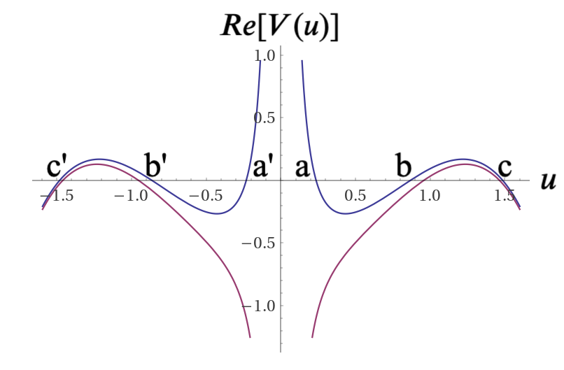
Figure 1: Plot of $Re[V(u)]$, from equation 26. In the upper figures the values of the constants are: $\eta_{\Lambda}=1/3$, $\eta_{c}=1$, $\eta_{s}=-0.03$, and $\eta_{r}=0.6$. In the lower figures the values of the constants are: $\eta_{\Lambda}=1/3$, $\eta_{c}=1$, $\eta_{s}=+0.03$, and $\eta_{r}=0.6$. Values of parameters taken from (Cordero ., 2019).

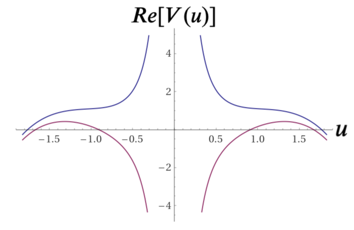
Figure 2: Plot of $Re[V(u)]$, from equation 26. In the upper figures the values of the constants are: $\eta_{\Lambda}=1/3$, $\eta_{c}=1$, $\eta_{s}=-0.468$, and $\eta_{r}=0.024$. In the lower figures the values of the constants are: $\eta_{\Lambda}=1/3$, $\eta_{c}=1$, $\eta_{s}=+0.468$, and $\eta_{r}=0.024$. Values of parameters taken from (Cordero ., 2019).

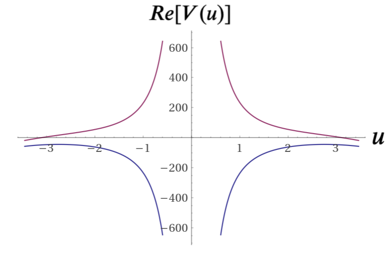
Figure 3: Plot of $Re[V(u)]$, from equation 26. In the upper figures the values of the constants are: $\eta_{\Lambda}=1/3$, $\eta_{c}=1$, $\eta_{s}=-234.0$, and $\eta_{r}=0$. In the lower figures the values of the constants are: $\eta_{\Lambda}=1/3$, $\eta_{c}=1$, $\eta_{s}=+234.0$, and $\eta_{r}=0$. Values of parameters taken from (Cordero ., 2019).

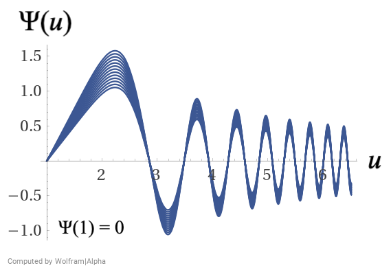
Figure 4: Plot of a family of solutions of Equation 23 with initial condition $\Psi(1)=0$. The values of the constants are: $\eta_{\Lambda}=1/3$, $\eta_{c}=1$, $\eta_{s}=+0.03$, and $\eta_{r}=0.6$. Values of parameters taken from (Cordero ., 2019).

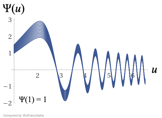
Figure 5: Plot of a family of solutions of Equation 23 with initial condition $\Psi(1)=1$. The values of the constants are: $\eta_{\Lambda}=1/3$, $\eta_{c}=1$, $\eta_{s}=+0.03$, and $\eta_{r}=0.6$. Values of parameters taken from (Cordero ., 2019).

In Figure (1) we sketch the behavior of the real part of the potential given by the equation 26 in two extreme cases, corresponding to $\eta_{s}>0$ and $\eta_{s}<0$. The values of the parameters were taken from (Cordero ., 2019) and correspond to typical values of approaches to formulating the Wheeler-DeWiit equation based on general relativity. The treated cases present a kind of potential barrier whose overcoming can occur in the form of quantum tunneling. In the case of the upper figures, both universes, in the contraction and expansion phases, in the case of no quantum tunneling, oscillate around two points of intersection with the horizontal axis, a’ and b’ and a and b, respectively. Morover, the upper figures exhibit infinite potential barriers that prevent the transition between the two phases, except in the case of a quantum leap. The lower figures do not present this infinite potential barrier but singularities. In the upper figures, singularities are suppressed.

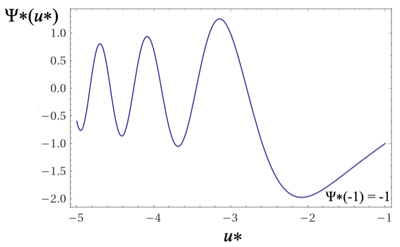
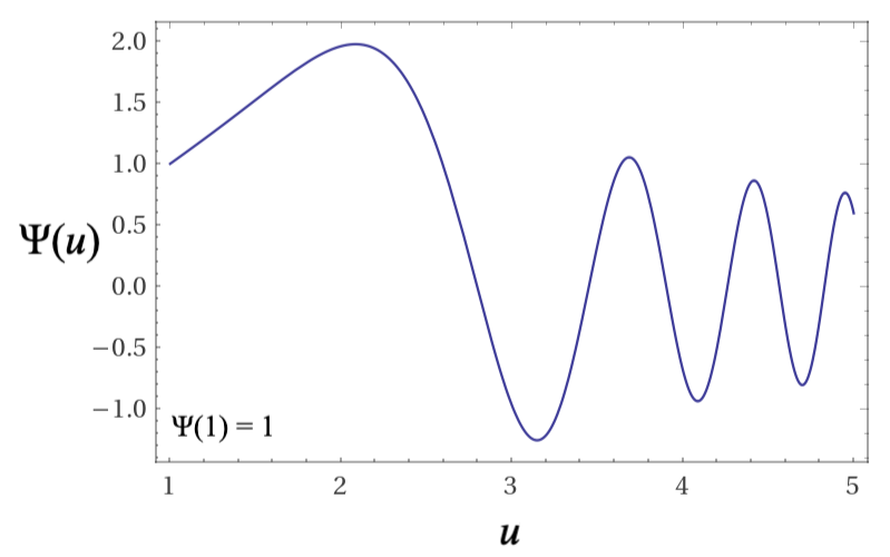
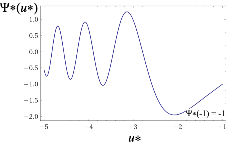
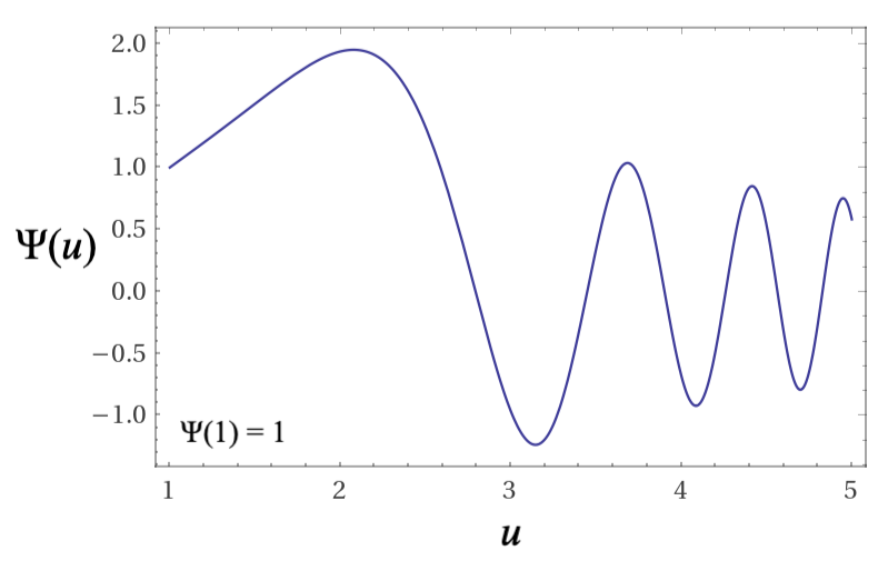
Figure 6: In the figures, plot of typical solutions of Equations 23 and 31 with boundary condition $\Psi(-1)=-1$ on the negative sector and $\Psi(1)=1$ on the positive sector. The values of the constants on the figures on the left are: $\eta_{\Lambda}=1/3$, $\eta_{c}=1$, $\eta_{s}=-0.03$, and $\eta_{r}=0.6$. In the figures on the right, the values of the constants are: $\eta_{\Lambda}=1/3$, $\eta_{c}=1$, $\eta_{s}=0.03$, and $\eta_{r}=0.6$. Values of parameters taken from (Cordero ., 2019).

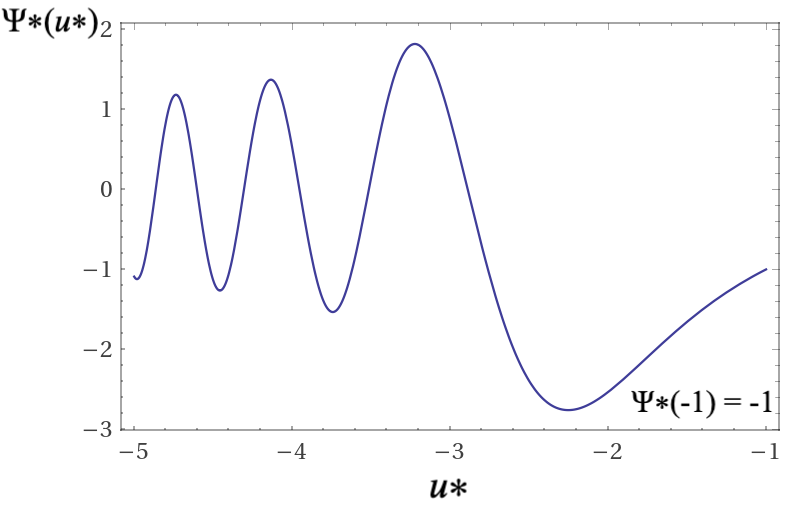
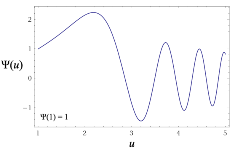
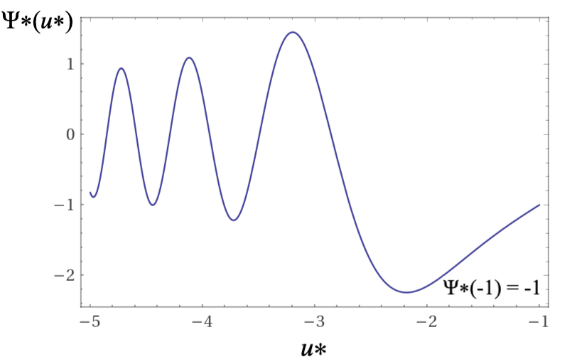
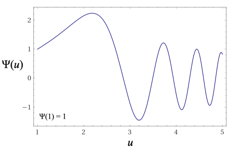
Figure 7: In the figures, plot of typical solutions of Equations 23 and 31 with boundary condition $\Psi(-1)=-1$ on the negative sector and $\Psi(1)=1$ on the positive sector. The values of the constants on the figures on the left are: $\eta_{\Lambda}=1/3$, $\eta_{c}=1$, $\eta_{s}=-0.468$, and $\eta_{r}=0.024$. In the figures on the right, the values of the constants are: $\eta_{\Lambda}=1/3$, $\eta_{c}=1$, $\eta_{s}=+0.468$, and $\eta_{r}=0.024$. Values of parameters taken from (Cordero ., 2019).

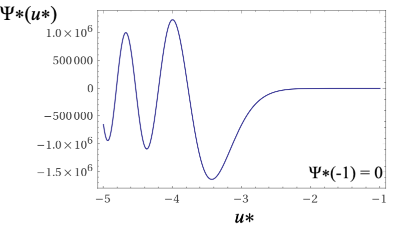
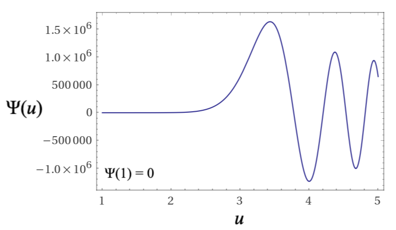
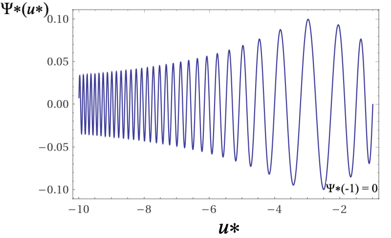
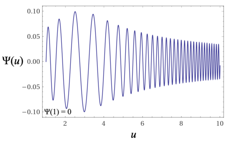
Figure 8: In the figures, plot of typical solutions of Equations 23 and 31 with boundary condition $\Psi(-1)=0$ on the negative sector and $\Psi(1)=0$ on the positive sector. The values of the constants on the figures on the left are: $\eta_{\Lambda}=1/3$, $\eta_{c}=1$, $\eta_{s}=-234.0$, and $\eta_{r}=0$. In the figures on the right, the values of the constants are: $\eta_{\Lambda}=1/3$, $\eta_{c}=1$, $\eta_{s}=+234.0$, and $\eta_{r}=0$. Values of parameters taken from (Cordero ., 2019).

4.1 Complex conjugate wave equations

In the branch-cut cosmology, the Friedmann-type equations analytically continued to the complex plane are (Zen Vasconcellos ., 2020, 20212, 20211):

$$\Biggl{(}\frac{\frac{d}{dt}\ln^{-1}[\beta(t)]}{\ln^{-1}[\beta(t)]}\Biggr{)}^{2}=\frac{8\pi G}{3}\rho(t)-\frac{kc^{2}}{\ln^{-1}[\beta(t)]}+\frac{1}{3}\Lambda\,;$$ (27)

and

$$\Biggl{(}\frac{\frac{d^{2}}{dt^{2}}\ln^{-1}[\beta(t)]}{\ln^{-1}[\beta(t)]}\Biggr{)}=-\frac{4\pi G}{3}\Big{(}\rho(t)+\frac{3}{c^{2}}p(t)\Bigr{)}+\frac{1}{3}\Lambda,$$ (28)

where $\Lambda$ represents the cosmological constant. The corresponding complex conjugated Friedmann’s-type equations are:

$$\Biggl{(}\frac{\frac{d}{dt}\ln^{-1}(\beta^{*}(t^{*}))}{\ln^{-1}(\beta^{*}(t^{*}))}\Biggr{)}^{2}=\frac{8\pi G}{3}\rho^{*}(t^{*})-\frac{kc^{2}}{\ln^{-2}(\beta^{*}(t^{*}))}+\frac{1}{3}\Lambda^{*},$$ (29)

and

$$\Biggl{(}\frac{\frac{d^{2}}{dt^{*2}}\ln^{-1}(\beta^{*}(t^{*}))}{\ln^{-1}(\beta^{*}(t^{*}))}\Biggr{)}=-\frac{4\pi G}{3}\Biggl{(}\rho^{*}(t^{*})+\frac{3}{c^{2}}p^{*}(t^{*})\Biggr{)}+\frac{1}{3}\Lambda^{*}.$$ (30)

Following a similar procedure, in this work we consider the complex conjugate version of equation (23)

$$\Biggl{(}-\frac{d^{2}}{du^{*2}}+\eta_{c}u^{*2}-\eta_{\Lambda}u^{*4}-\eta_{r}-\frac{\eta_{s}}{u^{*2}}\Biggr{)}\Psi^{*}(u^{*})=0\,.$$ (31)

4.2 Solutions and Boundary Conditions

The most known proposals for the boundary conditions of the wave-function of the universe are the “no boundary” (Hartle  Hawking, 1983) and tunneling boundary conditions (Vilenkin, 1982). These boundary conditions, although based on different conceptions and assumptions, have in common the prediction of an inflationary stage of evolution of the Universe. According to the singularity theorems of Hawking and Penrose, the universe would not have a classical beginning corresponding to a Lorentzian geometry, but would have started based on a regular Euclidean geometry with four spatial dimensions, followed by a quantum transition to a Lorentzian geometry with a temporal and three spatial dimensions (Hawking, 1982). The tunneling boundary condition of Vilenkin (1986) has two degrees of freedom: the scale factor and a homogeneous scalar field. A tunneling wave function then describes an ensemble of universes tunneling from “nothing” to a de Sitter space, and then evolving along the lines of an inflationary scenario and eventually collapsing to a singularity (Vilenkin, 1986).

In this contribution, we present a different proposal, as we will see below, in order to reconcile the evolutionary behavior of the branch-cut universe in the anterior and posterior regions dominated by Planck dimensions.

In Figures 4 and 5 we show a family of solutions of Equation 23, considering a real potential, for the positive region of evolution of the branch-cut universe. The values of the constants are: $\eta_{\Lambda}=1/3$, $\eta_{c}=1$, $\eta_{s}=+0.03$, and $\eta_{r}=0.6$. The boundary conditions correspond to $y(1)=1$ and $y(1)=0$, as for values of $x$ between 0 and 1 the equation has no solution. In the case where $x$ is negative, the solutions are similar but inverted, with a region between $x=-1$ and $x=1$ where the system of equations has no solution, which can be interpreted as the region where a quantum leap of the universe’s wave function occurs. The numerical values correspond to natural units, and the factor $1$ can be interpreted as a Planck unit of length, or, in view of the Bekenstein criterion, the smallest unit of length corresponding to the region in which the criterion is satisfied. In Figures 6, 7, and 8, we show typical solutions of Equations 23 and 31. The boundary conditions are $\Psi(-1)=-1$ or $\Psi(-1)=0$ on the negative sector, depending of the degree of convergence of the equations and $\Psi(1)=1$ or $\Psi(1)=0$ on the positive sector with the parameters taken from (Cordero ., 2019). As shown in the figures, for the region domains between $u=-1$ and $u=1$ the equations 23 and 31 have no solution. In our interpretation, this domain corresponds to the region in which a topological quantum leap occurs in accordance with the Bekenstein criterion (de Freitas Pacheco ., 2023; Bodmann ., 2023).

At this point, a word of caution regarding the choice of parameters. In this work we seek to adopt more conventional values of parameters, standards we could say, focusing more on the structural aspects of the branch-cut cosmology solutions in order to facilitate comparisons with more conventional approaches. In the future, we intend to focus on the issue of parametric choices, adopting specific procedures, more in line with the concepts proposed by the model. In this research work we adopted the choices made by Cordero . (2019). For their choices, the authors considered different scenarios for the universe and for the potentials in the Wheeler-DeWitt equation: with an embryonic epoch, with a potential barrier and no embryonic epoch, without a potential barrier and a big bounce, with an initial singularity of the primordial universe and no potential barrier (for more details see (Cordero ., 2019)).

5 Final remarks

Given the Klein-Gordon equation for a particle with mass $m$

$$\Bigl{(}\partial_{\mu}\partial^{\mu}+m^{2}\Bigr{)}\Phi(x)=0\,,$$ (32)

in covariant notation, the four-current (4) of the Klein-Gordon equation may be written as

$$j^{\mu}(x)=i\Bigl{[}\Phi^{*}(x)\partial^{\mu}\Phi(x)-\Bigl{(}\partial^{\mu}\Phi^{*}(x)\Bigr{)}\Phi(x)\Bigr{]}.$$ (33)

Combining (32) and (33), $\partial_{\mu}j^{\mu}(x)=0$, so the four-current $j^{\mu}(x)$ is a conserved quantity. However, the density

$$\rho(x)=i\Bigl{[}\Phi^{*}(x)\frac{\partial\Phi(x)}{\partial t}-\Bigl{(}\frac{\partial\Phi^{*}(x)}{\partial t}\Bigr{)}\Phi(x)\Bigr{]},$$ (34)

and the corresponding inner product

$$\langle\Phi_{1}(x)|\Phi_{2}(x)\rangle=\frac{i}{2}\int_{{\cal R}^{3}}d^{3}x\Bigl{[}\Phi_{2}(x)\frac{\partial\Phi_{1}(x)}{\partial t}-\Bigl{(}\frac{\partial\Phi_{2}(x)}{\partial t}\Bigr{)}\Phi_{1}(x)\Bigr{]}\,,$$ (35)

are not positive defined, so the Klein-Gordon wave function cannot therefore be interpreted as a probability amplitude. Moreover, endowing the vector space ${\cal V}$ of solutions of the Klein-Gordon equation with the “inner product” given by equation (35) does not generate a genuine inner product space. A similar problem arises in handling the Wheeler-DeWitt equation due to its Klein-Gordon structure, generating divergent interpretations about a probabilistic interpretation of the wave function of the universe.

In this work, we do not intend to focus on the nature of these interpretations, but rather focus on some still open questions that may shed some light on the contribution about this topic the branch-cut cosmology can offer. For example, going back to the Wheeler-DeWitt equation and the non-definite positiveness of its inner product, a way out of this problem would be to restrict the domain of the inner product to a subspace of quantum state vectors that correspond to positive energy solutions. This procedure makes it possible to obtain a definite positive inner product that can be extended to a separable Hilbert space by means of Cauchy completion (see Mostafazadeh  Zamani (2006) and references therein).

Another way of examining the same problem corresponds to the quantum field theory domain, in which solutions of the Klein-Gordon equation are quantized and turned out to field operators, supplying the formulation with a second quantization methodology. In this case, while the branch-cut equation can describe the evolution of quantum states “with negative probability of realization”, the quantum field theory procedure describes the evolution of field operators associated to real and underlying virtual universes.

More specifically, instead of seeking the realization of an explicit manifestly covariant description for a positive-definite and Lorentz-invariant inner product on the space of solutions of the Wheeler-DeWitt equation, with may adopt a description based on a kind of ‘third’ quantization. In this procedure, we may complement the branch-cut wave function, solution of a formulation in the style of the Wheeler-DeWitt equation, with an operator structure of creation and annihilation operators of many universes. In short, while in quantum field theory, solutions to the Klein-Gordon equation are quantized and transformed into field operators, following a similar procedure, the $\Psi(u)$ solution of the branch-cut equation developed in the style of the Wheeler-DeWitt formulation, could be quantized and transformed into an operator that creates and annihilates universes, similarly to conventional particle creation and annihilation operators. The challenge of this proposition is to determine observables that quantify and justify this approach.

Hawking’s interpretative proposal (Hartle  Hawking, 1983), in turn, assumes that $|\Psi[h_{ij},\Phi,\Sigma)|^{2}$ is proportional to the probability $P_{\cal V}$ to find the universe in a constrained to a region configuration ${\cal V}$ of a superspace that contains a three-surface $\Sigma$, where the metric is described by $h_{ij}$ and matter fields represented by $\Phi$:

$$P_{\cal V}\propto\int_{{\cal V}}\Psi^{*}[h_{ij},\Phi,\Sigma)]\Psi[h_{ij},\Phi,\Sigma)]d{\cal V}\,.$$ (36)

An attractive possibility would be to seek an interpretation that presents points of similarity with the view of Hartle  Hawking (1983) for the wave function of the universe, adapting it to those aspects that are inherent to branch-cut cosmology.

In this interpretative search, however, we found also close contact points of the branch-cut cosmology with the Many-Worlds Interpretation of Quantum Mechanics, going back to Hugh Everett III (1956). According to him, there would be myriads of worlds in the Universe beyond the world we know. And when a quantum experiment with different possible outcomes is performed, all the outcomes are then realized, each of which is materialized in a newly created different world, even if we are only aware of the outcomes obtained in the world we live in.

The classical solution of the branch-cut cosmology, given by the complex form factor $\ln[\beta(t)]$, which corresponds to a helix-like superposition of cut-planes, maps an infinite number of Riemann sheets onto horizontal strips, which represent the complex time evolution of horizon sizes. The patch sizes in turn maps progressively the various branches of the $\ln[\beta(t)]$ function which are glued along the copies of each upper-half plane with their copies on the corresponding lower-half planes. In the branch-cut cosmology, the cosmic singularity is replaced by a family of Riemann sheets in which the scale factor shrinks to a finite critical size, — the range of $\ln^{-1}[\beta(t)]$, associated to the cuts in the branch cut, shaped by the $\beta(t)$ function —, well above the Planck length. In the contraction phase, as the patch size decreases with a linear dependence on $\ln[\beta(t)]$, light travels through geodesics on each Riemann sheet, circumventing continuously the branch-cut, and although the horizon size scale with $\ln^{\epsilon}[\beta(t)]$, the length of the path to be traveled by light compensates for the scaling difference between the patch and horizon sizes. Under these conditions, causality between the horizon size and the patch size may be achieved through the accumulation of branches in the transition region between the present state of the universe and the past events. In the branch-cut cosmology conception, the cosmological arrow of time is determined as the direction in which “time”, from the macroscopic point of view, flows globally. In the branch-cut cosmology, in turn, this local component is identified with the corresponding real local time component that results from the complexification of the FLRW metric  (Bodmann ., 2023).

Following previous proposals, $\Psi(\ln[\beta(t)])$ may be interpreted as the probability amplitude and its modulus square as the probability density distribution of universes for a given family of branches characterized by the complex form factor $\ln[\beta(t)]$. The wave function shows oscillations, i.e., its absolute value has maxima, so the corresponding values of $\ln[\beta(t)]$ are the most probable universes constricted to the branches $|\ln[\beta(t)]|$. Thus, there is a quasi-discrete distribution of universes corresponding to different value of the complex branch-cut form factor. The results also indicate that the wave function is suppressed toward small $|\ln[\beta(t)]|$ which may imply that very small universes are suppressed.

Many relevant questions involving the quantum version of branch-cut cosmology are still open, such as the role of complex potentials, the presence of higher spatial curvature terms in the formulation, the quantization of helix-type solutions, more in tune with the classical formulation, a more consistent evolution mapping of the cut-planes, the consequences of adopting a non-symmetric approach and a different ordering of the dimensionless thermodynamics connection $\epsilon$, the role of dark matter in the evolution of the branch-cut universe, the role of fluctuations in the primordial spectrum and seeds in the the early universe, and also questions regarding the multiverse content, as well as a class of solutions with ordering parameters (see Vieira . (2020)) among others.

6 Acknowledgements

P.O.H. acknowledges financial support from PAPIIT-DGAPA (IN100421). The authors wish to thank the referees for valuable comments.

References

- Arnowitt \BOthers. (\APACyear2004) \APACinsertmetastarADM{APACrefauthors}Arnowitt, R., Deser, S.\BCBL \BBA Misner, C. \APACrefYearMonthDay2004, \APACrefbtitleThe Dynamics of General Relativity. The Dynamics of General Relativity. \APACrefnotearXiv:gr-qc/0405109 \PrintBackRefs\CurrentBib
- Bertolami \BBA Zarro (\APACyear2011) \APACinsertmetastarBertolami2011{APACrefauthors}Bertolami, O.\BCBT \BBA Zarro, C\BPBIA. \APACrefYearMonthDay2011, \APACjournalVolNumPagesPhys. Rev. D84044042. \PrintBackRefs\CurrentBib
- Bodmann \BOthers. (\APACyear2023) \APACinsertmetastarZen2023b{APACrefauthors}Bodmann, B., Zen Vasconcellos, C\BPBIA., de Freitas Pacheco, J\BPBIA., Hess, P\BPBIO.\BCBL \BBA Hadjimichef, D. \APACrefYearMonthDay2023, \APACjournalVolNumPagesAstronomische Nachrichten. \APACrefnoteTo be published. \PrintBackRefs\CurrentBib
- Chojnacki \BBA Kwapisz (\APACyear2021) \APACinsertmetastarChojnacki{APACrefauthors}Chojnacki, J.\BCBT \BBA Kwapisz, J. \APACrefYearMonthDay2021, \APACjournalVolNumPagesPhys.Rev.D104103504. \PrintBackRefs\CurrentBib
- Cordero \BOthers. (\APACyear2019) \APACinsertmetastarCordero2019{APACrefauthors}Cordero, R., Garcia-Compean, H.\BCBL \BBA Turrubiates, F\BPBIJ. \APACrefYearMonthDay2019, \APACjournalVolNumPagesGeneral Relativity and Gravitation51138. \PrintBackRefs\CurrentBib
- de Freitas Pacheco \BOthers. (\APACyear2023) \APACinsertmetastarZen2023a{APACrefauthors}de Freitas Pacheco, J\BPBIA., Zen Vasconcellos, C\BPBIA., Hadjimichef, D., Hess, P\BPBIO.\BCBL \BBA Bodmann, B. \APACrefYearMonthDay2023, \APACrefbtitleBranch-Cut Cosmology and the Bekenstein Criterion. Branch-Cut Cosmology and the Bekenstein Criterion. \APACrefnoteTo be published by the Astronomische Nachrichten \PrintBackRefs\CurrentBib
- DeWitt (\APACyear1967) \APACinsertmetastarWDW{APACrefauthors}DeWitt, B\BPBIS. \APACrefYearMonthDay1967, \APACjournalVolNumPagesPhys. Rev.1601113. \PrintBackRefs\CurrentBib
- Everett III (\APACyear1956) \APACinsertmetastarEverett{APACrefauthors}Everett III, H. \APACrefYear1956. \APACrefbtitleThe Many-Worlds Interpretation of Quantum Mechanics The Many-Worlds Interpretation of Quantum Mechanics \APACtypeAddressSchool\BUPhD. \APACaddressSchoolPrinceton, USAPrinceton University Press. \PrintBackRefs\CurrentBib
- Everett III (\APACyear1957) \APACinsertmetastarEverett1957{APACrefauthors}Everett III, H. \APACrefYearMonthDay1957, \APACjournalVolNumPagesReviews of Modern Physics29 (3)454-462. \PrintBackRefs\CurrentBib
- Everett III (\APACyear1975 [1955]) \APACinsertmetastarEverett1955{APACrefauthors}Everett III, H. \APACrefYear1975 [1955], \APACrefbtitleThe Theory of the Universal Wave Function The Theory of the Universal Wave Function. \PrintBackRefs\CurrentBib
- Feinberg \BBA Peleg (\APACyear1995) \APACinsertmetastarFeinberg{APACrefauthors}Feinberg, J.\BCBT \BBA Peleg, Y. \APACrefYearMonthDay1995, \APACjournalVolNumPagesPhys.Rev. D521988. \PrintBackRefs\CurrentBib
- Flinn (\APACyear2020) \APACinsertmetastarFlinn{APACrefauthors}Flinn, G. \APACrefYear2020. \APACrefbtitleThe Wave Function of The Universe The Wave Function of The Universe \APACtypeAddressSchool\BUPhD. \APACaddressSchoolLondon, UKImperial College. \PrintBackRefs\CurrentBib
- Garattini \BBA Faizal (\APACyear2016) \APACinsertmetastarGarattini2016{APACrefauthors}Garattini, R.\BCBT \BBA Faizal, M. \APACrefYearMonthDay2016, \APACjournalVolNumPagesNuclear Physics B905313-326. \PrintBackRefs\CurrentBib
- García-Compeán \BBA Mata-Pacheco (\APACyear2022) \APACinsertmetastarCompean{APACrefauthors}García-Compeán, H.\BCBT \BBA Mata-Pacheco, D. \APACrefYearMonthDay2022, \APACjournalVolNumPagesUniverse8237. \PrintBackRefs\CurrentBib
- Hartle \BBA Hawking (\APACyear1983) \APACinsertmetastarHartle{APACrefauthors}Hartle, J.\BCBT \BBA Hawking, S\BPBIW. \APACrefYearMonthDay1983, \APACjournalVolNumPagesPhys. Rev. D282960. \PrintBackRefs\CurrentBib
- Hawking (\APACyear1982) \APACinsertmetastarHawking1982{APACrefauthors}Hawking, S. \APACrefYearMonthDay1982, \APACjournalVolNumPagesPontif. Acad. Sci. Scr. Varia48563. \PrintBackRefs\CurrentBib
- Hořava (\APACyear2009) \APACinsertmetastarHorava{APACrefauthors}Hořava, P. \APACrefYearMonthDay2009, \APACjournalVolNumPagesPhys. Rev. D79084008. \PrintBackRefs\CurrentBib
- i. Maeda \BOthers. (\APACyear2010) \APACinsertmetastarMaeda{APACrefauthors}i. Maeda, K., Misonoh, Y.\BCBL \BBA Kobayashi, T. \APACrefYearMonthDay2010, \APACjournalVolNumPagesPhys. Rev. D82. \PrintBackRefs\CurrentBib
- Kim (\APACyear1997) \APACinsertmetastarKim{APACrefauthors}Kim, S\BPBIP. \APACrefYearMonthDay1997, \APACjournalVolNumPagesPhys. Lett. A23611. \PrintBackRefs\CurrentBib
- Mostafazadeh \BBA Zamani (\APACyear2006) \APACinsertmetastarMostafazadeh{APACrefauthors}Mostafazadeh, A.\BCBT \BBA Zamani, F. \APACrefYearMonthDay2006, \APACjournalVolNumPagesAnnals of Physics321 (9)2183-2209. \PrintBackRefs\CurrentBib
- Mukohyama (\APACyear2009) \APACinsertmetastarMukohyama2009{APACrefauthors}Mukohyama, S. \APACrefYearMonthDay2009, \APACjournalVolNumPagesPhys. Rev. D80064005. \PrintBackRefs\CurrentBib
- Mukohyama (\APACyear2010) \APACinsertmetastarMukohyama{APACrefauthors}Mukohyama, S. \APACrefYearMonthDay2010, \APACjournalVolNumPagesClass. Quant. Grav.27223101. \PrintBackRefs\CurrentBib
- Plato (\APACyear[428 - 348 a.C.] 2004) \APACinsertmetastarPlato{APACrefauthors}Plato. \APACrefYearMonthDay[428 - 348 a.C.] 2004, \APACrefbtitlePlato - Stanford Encyclopedia of Philosophy. Plato - Stanford Encyclopedia of Philosophy. \APACrefnotehttps://plato.stanford.edu/entries/plato/ \PrintBackRefs\CurrentBib
- Rovelli (\APACyear2015) \APACinsertmetastarRovelli2015{APACrefauthors}Rovelli, C. \APACrefYearMonthDay2015, \APACjournalVolNumPagesClassical and Quantum Gravity32 (12)124005. \PrintBackRefs\CurrentBib
- Rovelli (\APACyear2019) \APACinsertmetastarRovelli2019{APACrefauthors}Rovelli, C. \APACrefYear2019, \APACrefbtitleThe Order of Time The Order of Time. \APACaddressPublisherNew York, USARiverhead Books. \PrintBackRefs\CurrentBib
- Rovelli \BBA Smerlak (\APACyear2011) \APACinsertmetastarRovelli2011{APACrefauthors}Rovelli, C.\BCBT \BBA Smerlak, M. \APACrefYearMonthDay2011, \APACjournalVolNumPagesClassical and Quantum Gravity28075007. \PrintBackRefs\CurrentBib
- Saridakis (\APACyear2010) \APACinsertmetastarSaridakis{APACrefauthors}Saridakis, E\BPBIN. \APACrefYearMonthDay2010, \APACrefbtitleAspects of Horava-Lifshitz cosmology. Aspects of Horava-Lifshitz cosmology. \APACrefnotearXiv:1101.0300 [astro-ph.CO] \PrintBackRefs\CurrentBib
- T. Shestakova (\APACyear2019) \APACinsertmetastarShestakova2019{APACrefauthors}Shestakova, T. \APACrefYearMonthDay2019, \APACjournalVolNumPagesInt. J. Mod. Phys. D28 (13)1941009. \PrintBackRefs\CurrentBib
- T\BPBIP. Shestakova (\APACyear2018) \APACinsertmetastarShestakova2018{APACrefauthors}Shestakova, T\BPBIP. \APACrefYearMonthDay2018, \APACjournalVolNumPagesInt. J. Mod. Phys. D271841004. \PrintBackRefs\CurrentBib
- Vakili \BBA Kord (\APACyear2013) \APACinsertmetastarVakili{APACrefauthors}Vakili, B.\BCBT \BBA Kord, V. \APACrefYearMonthDay2013, \APACjournalVolNumPagesGen. Rel. Grav.451313. \PrintBackRefs\CurrentBib
- Vieira \BOthers. (\APACyear2020) \APACinsertmetastarVieira{APACrefauthors}Vieira, H., Bezerra, V., Muniz, C., Cunha, M.\BCBL \BBA Christiansen, H. \APACrefYearMonthDay2020, \APACjournalVolNumPagesPhys. Lett. B809135712. \PrintBackRefs\CurrentBib
- Vilenkin (\APACyear1982) \APACinsertmetastarVilenkin{APACrefauthors}Vilenkin, A. \APACrefYearMonthDay1982, \APACjournalVolNumPagesPhys. Lett. B11725. \PrintBackRefs\CurrentBib
- Vilenkin (\APACyear1986) \APACinsertmetastarVilenkin1986{APACrefauthors}Vilenkin, A. \APACrefYearMonthDay1986, \APACjournalVolNumPagesPhys. Rev. D333560. \PrintBackRefs\CurrentBib
- Wiltshire (\APACyear1996) \APACinsertmetastarWiltshire{APACrefauthors}Wiltshire, D. \APACrefYear1996, \APACrefbtitleAn introduction to quantum cosmology An introduction to quantum cosmology (\BVOL 2; B. Robson, N. Visvanathan\BCBL \BBA W. Woolcock, \BEDS). \APACaddressPublisherSingaporeWorld Scientific Pub. Co. \PrintBackRefs\CurrentBib
- Zen Vasconcellos \BOthers. (\APACyear2022) \APACinsertmetastarZen2022{APACrefauthors}Zen Vasconcellos, C\BPBIA., Hadjimichef, D., Hess, P\BPBIO., de Freitas Pacheco, J\BPBIA.\BCBL \BBA Bodmann, B. \APACrefYearMonthDay2022, \APACrefbtitleEvidences for the Branch-Cut Cosmology. Evidences for the Branch-Cut Cosmology. \APACrefnoteXXI Meeting of Physics. UNSAAC, Cusco, Perú, 16-18 December 2021. To be published by Journal of Physics: Conference Series \PrintBackRefs\CurrentBib
- Zen Vasconcellos \BOthers. (\APACyear2020) \APACinsertmetastarZen2020{APACrefauthors}Zen Vasconcellos, C\BPBIA., Hadjimichef, D., Razeira, M., Volkmer, G.\BCBL \BBA Bodmann, B. \APACrefYearMonthDay2020, \APACjournalVolNumPagesAstronomische Nachrichten340 (9,10)857. \PrintBackRefs\CurrentBib
- Zen Vasconcellos \BOthers. (\APACyear2021\APACexlab\BCnt1) \APACinsertmetastarZen2021b{APACrefauthors}Zen Vasconcellos, C\BPBIA., Hess, P\BPBIO., Hadjimichef, D., Bodmann, B., Razeira, M.\BCBL \BBA Volkmer, G. \APACrefYearMonthDay2021\BCnt1, \APACjournalVolNumPagesAstronomische Nachrichten342 (5)776-787. \PrintBackRefs\CurrentBib
- Zen Vasconcellos \BOthers. (\APACyear2021\APACexlab\BCnt2) \APACinsertmetastarZen2021a{APACrefauthors}Zen Vasconcellos, C\BPBIA., Hess, P\BPBIO., Hadjimichef, D., Bodmann, B., Razeira, M.\BCBL \BBA Volkmer, G. \APACrefYearMonthDay2021\BCnt2, \APACjournalVolNumPagesAstronomische Nachrichten342 (5)765-775. \PrintBackRefs\CurrentBib