Adaptive Bayesian Beamforming for Imaging by
Marginalizing the Speed of Sound

Abstract

Imaging methods based on array signal processing often require a fixed propagation speed of the medium, or speed of sound (SoS)for methods based on acoustic signals. The resolution of the images formed using these methods is strongly affected by the assumed SoS, which, due to multipath, nonlinear propagation, and non-uniform mediums, is challenging at best to select. In this letter, we propose a Bayesian approach to marginalize the influence of the SoS on beamformers for imaging. We adapt Bayesian direction-of-arrival estimation to an imaging setting and integrate a popular minimum variance beamformer over the posterior of the SoS. To solve the Bayesian integral efficiently, we use numerical Gauss quadrature. We apply our beamforming approach to shallow water sonar imaging where multipath and nonlinear propagation is abundant. We compare against the minimum variance distortionless response (MVDR) beamformer and demonstrate that its Bayesian counterpart achieves improved range and azimuthal resolution while effectively suppressing multipath artifacts.

I Introduction

Bbeamforming algorithms [1, 2, 3] for imaging require accurate physical modeling of the system to achieve high resolution. Often it is assumed that the signal propagates in a linear “direct path” with a globally fixed propagation speed of the medium. This model is “wrong but useful”, as George Box would comment, but discrepancies between the actual physics and the model result in lower image resolution and artifacts [4]. For example, sonar imaging in shallow waters suffers from multipath artifacts [5], while ultrasound imaging has to deal with inhomogeneous media [6, 7]. Since we focus on applications with complex acoustic propagation (such as sonar, medical ultrasound, and seismology), with some loss of generality, we will hereafter refer to the propagation speed as the speed of sound (SoS).

Various approaches have been proposed to combat the issue of SoS selection. Some works have proposed to statistically estimate the propagation speed [8, 9], and some of these have been specifically proposed in the context of beamforming [7]. Although the method of Stahli et al. [8] provides pixel-wise estimates of the SoS, it requires a priori segmentation of the target field, and its utility for beamforming has yet to be studied. Meanwhile, adaptive beamformers such as variants of the MVDR beamformer, which are purely statistical signal processing-based approaches, [2, 10] have shown to be effective against SoS mismatch [4] and other inconveniences such as cross-channel interference, noise [11], and multipath [5].

In the context of target direction-of-arrival (DoA) estimation, Bell et al. [12] have proposed a Bayesian approach to robust adaptive beamforming. They perform Bayesian inference of the optimal beam steering direction, where the likelihood uses the covariance of the received signal. The posterior can be used to marginalize the steering direction used within the minimum-variance distortionless response (MVDR)beamformer [13]. The Bayesian robust adaptive (BRA)beamformer has been further extended for multiple DoA estimation [14] and passive sonar detection [15], while the convergence of this method has been established by Lam and Singer [16].

When applying beamforming to imaging, each pixel in the image becomes a focal target. Therefore, the DoA estimation framework cannot be directly applied. However, in this letter, we demonstrate that the DoA estimation framework can be used for pixel-wise SoS estimation. Firstly, we estimate the pixel-wise SoS by adopting the likelihood of the BRA beamformer. Then, the SoS used to compute the MVDR beamfomer is marginalized over the posterior for the SoS. Our approach provides a data-driven way to handle uncertainties associated with the propagation model by expressing them as uncertainties in the SoS. We also propose to solve the marginalizing integral using Gauss-Hermite quadrature. Compared to previous works in Bayesian DoA estimation, this enables the proper use of priors with continuous support such as the Gaussian distribution.

We evaluate our method by applying it to active sonar imaging. We use the Bellhop propagation model [17, 18] to simulate point targets. Compared to the MVDR beamformer [13, 11, 19, 20] popularly used in sonar imaging [21, 22, 23, 24, 25, 26], our method effectively suppresses multipath artifacts while achieving lower sidelobes and better azimuth resolution.

To summarize, the contributions of this letter are as follows:

• A Bayesian model for estimating the speed of sound from the received signal on a pixel-by-pixel basis (Sections II-B and II-C).

• The first adaptive beamforming algorithm for imaging that marginalizes the speed of sound over its posterior (Section II-E).

• A simple and efficient numerical quadrature scheme for computing the marginalized beamformer (Section II-D).

II Adaptive Bayesian Beamforming by Marginalizing of the Speed of Sound

II-A Background and Motivation

Conventional Beamforming

The conventional delay-and-sum (DAS, [3]) beamforming method, also known as backprojection, is described as

$$y\left(p\right)=\sum^{N_{\text{sens.}}}_{n=1}w_{n}\,x_{n}\big{(}t\,(p,c,n)\big{)}=\mathbf{w}^{\dagger}\mathbf{x}_{d}\left(p,c\right),$$ (1)

where $\dagger$ is the conjugate transpose, $x_{n}\left(t\right)$ is the signal sample received by the $n$th sensor at time $t$, $p$ is the focal point (or image pixel), $y\left(p\right)$ is the beamformed response of $p$, $c$ is the signal propagation speed of the medium, $n=1,\ldots,N_{\text{sens.}}$ is the sensor index, $t\left(p,c,n\right)$ is the round-trip time for the response of $p$ to reach the $n$th sensor, $w_{n}$ is known as the fading weight or apodization weight, $\mathbf{w}$ is the fading weight vector, and $\mathbf{x}_{d}\left(p,c\right)$ is the delayed signals in vector form.

The round-trip time $t\left(p,c,n\right)$ is computed as

$$t\left(p,c,n\right)=r\left(p,c,n\right)/c=\left(r_{\mathrm{TX}}\left(p,c\right)+r_{\mathrm{RX}}\left(p,c,n\right)\right)/c,$$ (2)

where $r\left(p,c,n\right)$ is the round-trip distance from the source to the $n$th array sensor, $r_{\mathrm{TX}}$ is the distance from source to the $p$, $r_{\mathrm{RX}}$ is the distance from $p$ to the array sensor. In this work, we consider a 2-dimensional imaging setting over the azimuth ($x$-axis) and range ($y$-axis).

Choosing the Speed of sound

Eq. 2 assumes that the signal propagates linearly at a constant speed $c$. Since many imaging systems use acoustic signals, with some loss of generality, we will refer to $c$ as the SoS. Choosing $c$ is crucial to the resolution of the resulting image [4, 7]. We assert that the common practice of choosing a globally fixed SoS is suboptimal. This is especially apparent in sonar applications where the propagation path is nonlinear and varies depending on oceanic parameters such as the SoS profile [27].

Speed of Sound and Multipath

Furthermore, active sonar suffers from multipath, where a signal traveling between two points can take multiple paths of different lengths. Under the direct-path model, this results in the SoS having multiple “optimal” values. This problem is visualized in Fig. 1. When choosing a single fixed SoS, multipath will result in the same target appearing in multiple positions. In this work, we avoid the problem of choosing one fixed SoS by considering a continuous distribution of probable SoS values.

Figure 1: Illustration of the problem with fixed speed of sound. The optimal speed of sound can vary depending on the bathymetry, speed of sound profile, and propagation path.

II-B Signal Model

Before presenting our Bayesian beamforming approach, we discuss our signal model. Let a signal be generated from a focal point $p$. The spectrum of this signal when received by an $N_{\text{sens.}}$ sensor array is modeled as

$$\mathbf{x}\left(\omega\right)=s\left(p,\omega\right)\mathbf{a}\left(p,c\right)+\mathbf{n}\left(p,\omega\right)$$ (3)

where $\omega$ is the frequency, $s$ is the envelope of the original target response, $\mathbf{a}\in\mathbb{C}^{N_{\text{sens.}}}$ is the steering vector defined as

$$\mathbf{a}\left(p,c\right)={\begin{bmatrix}\;e^{-j\,t\,\left(p,\,c,\,1\right)}&\ldots&e^{-j\,t\,\left(p,\,c,\,N_{\text{sens.}}\right)}\;\end{bmatrix}}^{\dagger}$$ (4)

for the time delay $t\left(p,c,n\right)$, and $\mathbf{n}\in\mathbb{C}^{N_{\text{sens.}}}$ is the multivariate interference and noise vector. The dependence on $c$ signifies that the response of the same focal point $p$ can take different paths, which are identified by $c$. Note that $c$ corresponds to the average SoS over the direct path (a 2D projection of the nonlinear path) and is not the SoS at a specific position.

The covariance of the received signal $\mathbf{\Sigma}_{\mathbf{x}}\in\mathbb{C}^{N_{\text{sens.}}\times N_{\text{sens.}}}$ is

$$\mathbf{\Sigma}_{\mathbf{x}}\left(p,c\right)=\sigma^{2}_{s}\left(p\right)\;\mathbf{a}\left(p,c\right)\mathbf{a}^{\dagger}\left(p,c\right)+\mathbf{\Sigma}_{\mathbf{n}}\left(p\right),$$ (5)

where $\mathbf{\Sigma}_{\mathbf{n}}\in\mathbb{C}^{N_{\text{sens.}}\times N_{\text{sens.}}}$ is the noise (and interference) covariance matrix. Note that if the data $x_{n}$ is pre-delayed in the time domain by $t\,\left(p,\,c,\,n\right)$, the steering vector is replaced by a vector of 1s.

II-C Probabilistic Model

Likelihood

We now describe our probabilistic model used to infer the SoS. Our likelihood is similar to that used by the BRA beamformer [12] and is described as

$$\mathcal{L}\left(c\right) =\prod^{N_{\text{sub.}}}_{l=1}\mathcal{N}\left(\mathbf{x}_{l}\left(p,c\right);\;\mathbf{0},\,\Sigma_{\mathbf{x}}\left(c,p\right)\right)$$ (6)

$$=\prod^{N_{\text{sub.}}}_{l=1}\frac{1}{\pi^{N_{\text{sub.}}}{\left|\,\mathbf{\Sigma}_{\mathbf{x}}\left(c,p\right)\,\right|}}\exp\left(-\mathbf{x}_{l}^{\dagger}\left(p,c\right)\mathbf{\Sigma}^{-1}\left(c\right)\mathbf{x}_{l}\left(p,c\right)\right)$$ (7)

$$\propto{{\left|\,\mathbf{\Sigma}_{\mathbf{x}}\left(p,c\right)\,\right|}}^{-N_{\text{sub.}}}\exp\left(-\sum^{N_{\text{sub.}}}_{l=1}\mathbf{x}_{l}^{\dagger}\left(p,c\right)\mathbf{\Sigma}^{-1}_{\mathbf{x}}\left(p,c\right)\mathbf{x}_{l}\left(p,c\right)\right),$$ (8)

where the data points $\mathbf{x}_{l}\left(p,c\right)\in\mathbb{C}^{L}$ are obtained by dividing the $N_{\text{sens.}}$ sensor array into $N_{\text{sub.}}=N_{\text{sens.}}-L+1$ overlapping subarrays such that $\mathbf{x}_{l}\left(p,c\right)={\big{[}\,x_{l+1}\;x_{l+2}\;\ldots\;x_{l+L-1}\,\big{]}}^{\top}.$ Note that we have omitted the argument $t\left(p,c,l\right)$ for clarity. By using the subarray scheme [11], we avoid cancellation between coherent signals and obtain multiple samples without considering a temporal window. It also guarantees that the estimated covariance matrix is full-rank under mild assumptions [11].

The determinant in Eq. 8 penalizes large, complex covariances, while the exponential term penalizes covariances that fail to explain the obtained data. Therefore, this likelihood selects values of $c$ that are both (i) consistent with the model (ii) and result in a small covariance. Since the exact expression for $\mathbf{\Sigma}_{\mathbf{x}}$ is unknown due to our lack of knowledge on $\mathbf{\Sigma}_{\mathbf{n}}$ and $\sigma^{2}_{s}$, further approximation is required.

Approximate Likelihood

From the definition of $\mathbf{\Sigma}_{\mathbf{x}}$ in Eq. 5, Bell et al. [12] have shown that the likelihood can be represented as

$$\mathcal{L}\left(c\right) \propto{\left(1+\sigma^{2}\beta\left(c\right)\right)}^{-N_{\text{sub.}}}$$ (9)

$$\quad\times\exp\left(\frac{N_{\text{sub.}}\,\sigma^{2}_{s}\,\beta^{2}\left(c\right)}{1+\sigma^{2}\beta\left(c\right)}\,\frac{\mathbf{a}^{\top}\mathbf{\Sigma}_{\mathbf{n}}^{-1}\left(\mathbf{c}\right)\widehat{\mathbf{\Sigma}}_{\mathbf{n}}^{-1}\left(\mathbf{c}\right)\mathbf{\Sigma}_{\mathbf{n}}^{-1}\left(\mathbf{c}\right)\mathbf{a}}{\beta^{2}\left(c\right)}\right)$$ (10)

where $\beta\left(c\right)=\mathbf{a}^{\dagger}\mathbf{\Sigma}_{\mathbf{n}}\mathbf{a}$. Note that we have dropped the parameter $p$ for clarity. To avoid dealing with $\mathbf{\Sigma}_{\mathbf{n}}$, Bell et al. propose to further approximate the likelihood as

$$\mathcal{L}\left(c\right)\mathchoice{\mathrel{\raise 0.96873pt\hbox{\hbox to0.0pt{\hbox{$\displaystyle\propto$}\hss}\lower 3.63206pt\hbox{$\displaystyle\sim$}}}}{\mathrel{\raise 0.96873pt\hbox{\hbox to0.0pt{\hbox{$\textstyle\propto$}\hss}\lower 3.63206pt\hbox{$\textstyle\sim$}}}}{\mathrel{\raise 0.67812pt\hbox{\hbox to0.0pt{\hbox{$\scriptstyle\propto$}\hss}\lower 2.54245pt\hbox{$\scriptstyle\sim$}}}}{\mathrel{\raise 0.48436pt\hbox{\hbox to0.0pt{\hbox{$\scriptscriptstyle\propto$}\hss}\lower 1.81602pt\hbox{$\scriptscriptstyle\sim$}}}}\exp\big{(}N_{\text{sub.}}\;\gamma\;P_{s}(c),\big{)}$$ (11)

where $P_{s}$ is the spectral estimate of the optimal output power $\sigma_{s}^{2}$ and $\gamma$ is a constant controlling the strength of the likelihood depending on the signal-to-noise (SNR) ratio.

The Capon [28] spectral estimate of the optimal output power is defined as

$$P_{s}\left(c\right)={\left(\mathbf{a}^{\dagger}{\mathbf{\Sigma}_{\mathbf{n}}}^{-1}\left(c\right)\mathbf{a}\right)}^{-1}$$ (12)

and is the only point where the data enters our likelihood. Therefore, accurately estimating $P_{s}$ is crucial to the performance of our beamformer. We further discuss this in Section II-D. Since $\mathbf{\Sigma}_{\mathbf{n}}\left(c\right)$ is a nonlinear function of $c$, our model is not linear unlike its mathematical appearance.

The power strength constant is defined as

$$\gamma=\frac{N_{\text{sub.}}}{\sigma_{n}^{4}}\,\frac{N_{\text{sub.}}\,\nicefrac{{\sigma^{2}_{s}}}{{\sigma^{2}_{n}}}}{1+N_{\text{sub.}}\,\nicefrac{{\sigma^{2}_{s}}}{{\sigma^{2}_{n}}}}=\frac{N_{\text{sub.}}}{\mathsf{NL}^{2}}\,\frac{N_{\text{sub.}}\,\mathsf{SNR}}{1+N_{\text{sub.}}\,\mathsf{SNR}},$$ (13)

where $\mathsf{SNR}=\nicefrac{{\sigma^{2}_{s}}}{{\sigma^{2}_{n}}}$ is the signal-to-noise ratio and $\mathsf{NL}=\sigma_{n}^{2}$ is the noise level.

Power Strength $\gamma$

While the original passive detection setting of Bell et al. allowed the use of a fixed $\mathsf{SNR}$ and $\mathsf{NL}$, this is not the case for our active imaging setting. In active imaging systems, the signal level (and thus the SNR) decreases with distance due to path loss. To compensate for this, a time-varying gain (TVG) gain is applied proportionally to the round-trip distance $r_{p}$. This results in the ambient noise level $\mathsf{NL}$ being amplified with distance. We thus define a focal point dependent $\gamma\left(p\right)$ comprised of

$$\mathsf{NL}\left(p\right)\texttt{[dB]} =\mathsf{DR}-\mathsf{SNR}_{0}+G_{\mathrm{TVG}}\left(r_{p}\right)$$ (14)

$$\mathsf{SNR}\left(p\right)\texttt{[dB]} =\mathsf{SNR}_{0}-\mathsf{PL}\left(p\right)\approx\mathsf{SNR}_{0}-G_{\mathrm{TVG}}\left(r_{p}\right),$$ (15)

where $\mathsf{DR}$ is the dynamic range, $\mathsf{SNR}_{0}$ is the optimal SNR, $\mathsf{PL}\left(p\right)$ and $G_{\mathrm{TVG}}\left(r_{p}\right)$ are the path loss and TVG for the focal point $p$. Note that Eq. 14 assumes that the signal tightly fits the dynamic range while Eq. 15 assumes that the TVG is set similarly to the path loss.

II-D Bayesian Inference

Spectral Estimation

Estimating $P_{s}$ is normally carried out by first substituting the empirical data covariance $\widehat{\mathbf{\Sigma}}_{\mathbf{x}}$ for the noise covariance $\mathbf{\Sigma}_{\mathbf{n}}$ such that $P_{s}\approx{\left(\mathbf{a}^{\dagger}\widehat{\mathbf{\Sigma}}_{\mathbf{x}}\mathbf{a}\right)}^{-1}$. For estimating the covariance, as discussed in Section II-C, we use subarray averaging [11], where the $N_{\text{sens.}}$-sensor array is divided into $N_{\text{sub.}}$ subarrays. This leads to an $N_{\text{sub.}}$-sample estimate of the covariance matrix,

$$\widehat{\mathbf{\Sigma}}_{\mathbf{x}}\left(p,c\right)=\frac{1}{L}\sum^{N_{\text{sub.}}}_{l=1}\mathbf{x}_{l}\left(p,c\right)\mathbf{x}^{\dagger}_{l}\left(p,c\right).$$ (16)

Without subarray averaging, cancellations of coherent signals result in a significant underestimation of the signal power, leading to our likelihood being underpowered. We thus use forward-backward averaging [29, 30, 31] as

$$\widehat{\mathbf{\Sigma}}_{\mathbf{x},\,\text{FB}}\left(p,c\right)=\frac{1}{2}\left(\widehat{\mathbf{\Sigma}}_{\mathbf{x}}\left(p,c\right)+\mathbf{J}\,{\widehat{\mathbf{\Sigma}}_{\mathbf{x}}^{\top}\left(p,c\right)}\,\mathbf{J}\right),$$ (17)

where $\mathbf{J}$ is the exchange matrix with only 1s in the anti-diagonal, and diagonal loading [19]

$$\widehat{\mathbf{\Sigma}}_{\mathbf{x},\,\text{DL}}\left(p,c\right)=\widehat{\mathbf{\Sigma}}_{\mathbf{x},\,\text{FB}}\left(p,c\right)+\epsilon\,\text{trace}\left\{\,\widehat{\mathbf{\Sigma}}_{\mathbf{x},\,\text{FB}}\left(p,c\right)\,\right\}\,\mathbf{I}$$ (18)

with $\epsilon=10^{-3}/N_{\text{sub.}}$ as recommended by Featherstone [32]. These modifications significantly improve the magnitude of the estimated power [20], which is crucial for our approach.

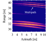
(a) DAS

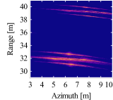
(b) MVDR

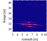
(c) Bayes $N_{\text{quad.}}$=8

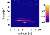
(d) Bayes $N_{\text{quad.}}$=32

Figure 3: Images formed by the methods considered in this work. The dynamic range is restricted to 60dB. Compared to MVDR, our proposed scheme (shown as “Bayes”) achieve lower sidelobes and fewer multipath artifacts.

Prior Distribution

For DoA estimation, it is natural to consider an uninformative prior on the steering angle. Furthermore, using a discrete distribution simplifies the computation associated with performing Bayesian inference. Thus, previous works [15, 14] considered to set a uniform discrete prior with a support of $[-\pi,\pi]$ on the steering angle.

For the speed of sound, we are in a slightly different position. (i) We have an informed guess about the optimal SoS, (ii) but do not know how much the true optimal SoS will deviate from it. Therefore, we consider a continuous informative prior distribution with “soft” boundaries. We choose the prior to follow a normal distribution as $\rho\left(c\right)=\mathcal{N}\left(c;\mu_{c},\sigma^{2}_{c}\right)$ with mean $\mu_{c}$ and standard deviation $\sigma_{c}$.

Inference with Gauss-Hermite Quadrature

By choosing a Gaussian prior, we can use Gauss-Hermite quadrature [33]. This provides a principled approach to computing the marginalizing integral (discussed in section II-E) without relying on arbitrary discretization as done in previous works [15, 14]. Given a computational budget of $N_{\text{q}}$ quadrature points, the posterior $\pi$ is

$$\pi\left(c\right) \propto\rho\left(c\right)\,\mathcal{L}\left(c\right)\propto\exp\left(-\frac{1}{2}\frac{{\left(c-\mu_{c}\right)}^{2}}{\sigma_{c}^{2}}\right)\,\mathcal{L}\left(c\right)$$

$$\propto e^{-z^{2}}\,\mathcal{L}\left(\sqrt{2}\,z\,\sigma_{c}+\mu_{c}\right),$$ (19)

where we have reparameterized $c=\sqrt{2}\,z\,\mu_{c}+\sigma_{c}$. From this parameterization, the posterior expectation (marginal) can be computed by setting $e^{-z^{2}}=u_{n}$ and $z=z_{n}$, where for $n=1,\ldots,N_{\text{quad.}}$, $z_{n}$ is the Gauss-Hermite quadrature node, and $u_{n}$ is the $n$th Gauss-Hermite weight.

II-E Marginalized Adaptive Beamformer

Figure 4: Normalized azimuth resolution plot for a target at 36m. The dotted line shows the position of the point target.

Given the posterior of $c$, we compute the marginalized MVDR beamformer as

$$y\left(p\right) =\int\mathbf{w}^{\dagger}\left(p,c\right)\,\mathbf{x}_{d}\left(p,c\right)\,\pi\left(c\right)\,dc$$ (20)

$$\approx\frac{1}{\sum^{N_{\text{quad.}}}_{n=1}v_{n}}\sum^{N_{\text{quad.}}}_{n=1}v_{n}\,\mathbf{w}^{\dagger}\left(p,c\right)\,\mathbf{x}_{d}\left(p,c\right),$$ (21)

where the unnormalized posterior density is

$$v_{n}=u_{n}\,\mathcal{L}\left(\sqrt{2}\,z_{n}\,\sigma_{c}+\mu_{c}\right),$$ (22)

and the MVDR fading weights adapted from data are given as

$$\mathbf{w}\left(p,c\right)=\frac{\widehat{\mathbf{\Sigma}}_{\mathbf{x},\,\text{DL}}^{-1}\left(p,c\right)\mathbf{1}}{\mathbf{1}^{\top}\widehat{\mathbf{\Sigma}}_{\mathbf{x},\,\text{DL}}^{-1}\left(p,c\right)\mathbf{1}}.$$ (23)

Since we pre-delay the data before estimating the covariance, as stated in Section II-B, the steering vector is set as $\mathbf{a}=\mathbf{1}$. Also, we reuse the covariance $\widehat{\mathbf{\Sigma}}_{\mathbf{x},\,\text{DL}}$ used to compute the likelihood in Eq. 22 for finding the MVDR weights in Eq. 23.

Simulation Settings Parameter Value Unit Max bathymetry depth 100 [m] Number of sensors 30 Length of array 1 [m] LFM  center frequency 30k [Hz] LFM  bandwidth 20k [Hz] LFM  duration 50$\mu$ [s] Ambient noise power 80 [dB^a ] Signal power 190 [dB^a ] Sampling frequency 500k [Hz] Sampling duration 0.3 [s]

• unit: re 1 $\mu$Pa at 1m

Figure 2: speed of sound profile (black). The red line (1519 m/s) is the value used for imaging.

III Evaluation

III-A Sonar Simulation Setup

Simulation Implementation

We apply our beamformer to active sonar imaging. We simulate point targets with the Bellhop propagation model [17, 18], with an implementation similar to Larsson and Gillard [34], where only a single “ping” is used. The simulation settings are shown in Section II-E, while the SoS profile is shown in Fig. 2. The bathymetry is set to be flat. The array and the linear frequency-modulated (LFM) source are at a depth of 70m, while the targets are at a depth of 90m. The beam resolution is evaluated with a single point target at a range of 36m, while 5 point targets, which are 1m apart, are arranged as a “cross” for qualitative evaluation.

After simulating propagation, the signal is quantized into 16 bit resolution. Then, we apply a time-varying gain of $G_{\mathrm{TVG}}\left(t\right)=20\log r\approx 20\log\left(\pi t\,c\right)$ [dB], and demodulate the signal with a quadrature demodulator with a decimation ratio of 4. Range compression is then done by matched filtering.

Baselines and Algorithm Setup

For the baselines, we use the DAS beamformer and the MVDR adaptive beamformer [13]. Both use a constant SoS of 1519m/s. The DAS beamformer uses Hann fading weights. For the MVDR beamformer, we use subarray averaging, diagonal loading, and forward-backward averaging. We use $N_{\text{sub.}}=N_{\text{sens}}/2$ for both the MVDR beamfomer and our Bayesian beamformer. Lastly, for our Bayesian approach, we use $\text{SNR}_{0}=15$ dB and $\mu_{c}=1519,\sigma_{c}=0.3$.

III-B Simulation Results

Qualitative Results

The qualitative results are shown in Fig. 3. The 5 point targets forming a “cross” are near the range of 32m, while multipath artifacts appear near the range of 39m. In terms of resolution, our marginalized beamformer (Bayes) results in lower sidelobes compared to the DAS and MVDR beamformer, resulting in better visibility of the targets. Also, it suppresses the multipath artifacts more effectively compared to the other baselines.

Meanwhile, the difference in the performance of our method for larger numbers of quadrature points ($N_{\text{quad.}}=32$ versus $N_{\text{quad.}}=8$) is marginal. Quantitatively, the root mean squared error between the two is only -39.13dB. Therefore, the benefits of our beamformer can be enjoyed with a relatively small number of quadrature points. Moreover, increasing the number of quadrature points does not necessarily lead to increased resolution, as it is effectively adding signals.

TABLE I: Resolution and Multipath Artifact Suppression

	DAS	MVDR	Bayes (ours)	Bayes (ours)
			$N_{\text{quad.}}=8$	$N_{\text{quad.}}=32$
FWHM1 [m]	2.31	0.34	0.26	0.28
PMAL2 [dB]	-9.97	-9.44	-24.04	-24.41

• Full width at half maximum

• Peak multipath artifact level

Quantitative Results

The beam resolutions are visualized in Fig. 4, while the objective metrics are organized in Table I. Our marginalized beamformer (Bayes) can be seen to achieve better resolution compared to the DAS and MVDR beamformers. Furthermore, it achieves multipath artifact levels 14dB lower than the baselines.

IV Conclusions

In this work, we have presented a Bayesian adaptive beamformer for imaging that marginalizes the speed of sound. On simulated active sonar data, our beamformer achieved better resolution and improved suppression of multipath artifacts relative to DAS and MVDR beamformers. Our method applies to any array-based imaging method, including sonar imaging, medical ultrasound, and seismic imaging. For future directions, incorporating various uncertainties in the signal processing chain into a Bayesian model would be interesting.

References

- [1] W. Knight, R. Pridham, and S. Kay, “Digital signal processing for sonar,” Proceedings of the IEEE, vol. 69, no. 11, pp. 1451–1506, 1981.
- [2] B. Van Veen and K. Buckley, “Beamforming: A versatile approach to spatial filtering,” IEEE ASSP Magazine, vol. 5, no. 2, pp. 4–24, Apr. 1988.
- [3] H. L. Van Trees, Optimum array processing, ser. Detection, estimation, and modulation theory. New York, NY: Wiley, 2002, no. 4.
- [4] I. K. Holfort, F. Gran, and J. A. Jensen, “Investigation of sound speed errors in adaptive beamforming,” in 2008 IEEE Ultrasonics Symposium. Beijing, China: IEEE, Nov. 2008, pp. 1080–1083.
- [5] A. E. A. Blomberg, A. Austeng, R. E. Hansen, and S. A. V. Synnes, “Improving sonar performance in shallow water using adaptive beamforming,” IEEE Journal of Oceanic Engineering, vol. 38, no. 2, pp. 297–307, Apr. 2013.
- [6] G. F. Pinton, G. E. Trahey, and J. J. Dahl, “Sources of image degradation in fundamental and harmonic ultrasound imaging using nonlinear, full-wave simulations,” IEEE Transactions on Ultrasonics, Ferroelectrics and Frequency Control, vol. 58, no. 4, pp. 754–765, Apr. 2011.
- [7] V. Perrot, M. Polichetti, F. Varray, and D. Garcia, “So you think you can DAS? A viewpoint on delay-and-sum beamforming,” Ultrasonics, vol. 111, p. 106309, Mar. 2021.
- [8] P. Stahli, M. Frenz, and M. Jaeger, “Bayesian approach for a robust speed-of-sound reconstruction using pulse-echo ultrasound,” IEEE Transactions on Medical Imaging, vol. 40, no. 2, pp. 457–467, Feb. 2021.
- [9] R. Ali, A. V. Telichko, H. Wang, U. K. Sukumar, J. G. Vilches-Moure, R. Paulmurugan, and J. J. Dahl, “Local sound speed estimation for pulse-echo ultrasound in layered media,” IEEE Transactions on Ultrasonics, Ferroelectrics, and Frequency Control, vol. 69, no. 2, pp. 500–511, Feb. 2022.
- [10] H. Krim and M. Viberg, “Two decades of array signal processing research: the parametric approach,” IEEE Signal Processing Magazine, vol. 13, no. 4, pp. 67–94, Jul. 1996.
- [11] T.-J. Shan and T. Kailath, “Adaptive beamforming for coherent signals and interference,” IEEE Transactions on Acoustics, Speech, and Signal Processing, vol. 33, no. 3, pp. 527–536, Jun. 1985.
- [12] K. Bell, Y. Ephraim, and H. Van Trees, “A Bayesian approach to robust adaptive beamforming,” IEEE Transactions on Signal Processing, vol. 48, no. 2, pp. 386–398, Feb. 2000.
- [13] O. Frost, “An algorithm for linearly constrained adaptive array processing,” Proceedings of the IEEE, vol. 60, no. 8, pp. 926–935, 1972.
- [14] S. Chakrabarty and E. A. P. Habets, “A Bayesian approach to informed spatial filtering with robustness against DOA estimation errors,” IEEE/ACM Transactions on Audio, Speech, and Language Processing, vol. 26, no. 1, pp. 145–160, Jan. 2018.
- [15] B. A. Yocom, B. R. La Cour, and T. W. Yudichak, “A Bayesian approach to passive sonar detection and tracking in the presence of interferers,” IEEE Journal of Oceanic Engineering, vol. 36, no. 3, pp. 386–405, Jul. 2011.
- [16] C. Lam and A. Singer, “Bayesian beamforming for DOA uncertainty: Theory and implementation,” IEEE Transactions on Signal Processing, vol. 54, no. 11, pp. 4435–4445, Nov. 2006.
- [17] M. B. Porter and H. P. Bucker, “Gaussian beam tracing for computing ocean acoustic fields,” The Journal of the Acoustical Society of America, vol. 82, no. 4, pp. 1349–1359, Oct. 1987.
- [18] H. P. Bucker, “A simple 3‐D Gaussian beam sound propagation model for shallow water,” The Journal of the Acoustical Society of America, vol. 95, no. 5, pp. 2437–2440, May 1994.
- [19] B. Carlson, “Covariance matrix estimation errors and diagonal loading in adaptive arrays,” IEEE Transactions on Aerospace and Electronic Systems, vol. 24, no. 4, pp. 397–401, Jul. 1988.
- [20] B. M. Asl and A. Mahloojifar, “Contrast enhancement and robustness improvement of adaptive ultrasound imaging using forward-backward minimum variance beamforming,” IEEE Transactions on Ultrasonics, Ferroelectrics and Frequency Control, vol. 58, no. 4, pp. 858–867, Apr. 2011.
- [21] S. Stergiopoulos, “Implementation of adaptive and synthetic-aperture processing schemes in integrated active-passive sonar systems,” Proceedings of the IEEE, vol. 86, no. 2, pp. 358–398, Feb. 1998.
- [22] P. Gerstoft, W. Hodgkiss, W. Kuperman, Heechun Song, M. Siderius, and P. Nielsen, “Adaptive beamforming of a towed array during a turn,” IEEE Journal of Oceanic Engineering, vol. 28, no. 1, pp. 44–54, Jan. 2003.
- [23] A. E. A. Blomberg, “Adaptive beamforming for active sonar imaging,” Doctoral Thesis, University of Oslo, 2012.
- [24] A. Austeng, A. C. Jensen, C.-I. C. Nilsen, H. J. Callow, and R. E. Hansen, “Use of the minimum variance beamformer in synthetic aperture sonar imaging,” ser. ECUA’12, Edinburgh, Scotland, 2013, p. 070098.
- [25] J. I. Buskenes, J. P. Asen, C.-I. C. Nilsen, and A. Austeng, “An optimized GPU implementation of the MVDR beamformer for active sonar imaging,” IEEE Journal of Oceanic Engineering, vol. 40, no. 2, pp. 441–451, Apr. 2015.
- [26] J. I. Buskenes, R. E. Hansen, and A. Austeng, “Low-complexity adaptive sonar imaging,” IEEE Journal of Oceanic Engineering, pp. 1–10, 2016.
- [27] M. A. Ainslie, Principles of sonar performance modelling, ser. Springer Praxis books in geophysical sciences. Heidelberg [Germany] London New York Chichester, UK: Springer Published in association with Praxis Pub, 2010.
- [28] J. Capon, “High-resolution frequency-wavenumber spectrum analysis,” Proceedings of the IEEE, vol. 57, no. 8, pp. 1408–1418, 1969.
- [29] J. E. Evans, D. F. Sun, and J. R. Johnson, “Application of Advanced Signal Processing Techniques to Angle of Arrival Estimation in ATC Navigation and Surveillance Systems,” MIT Lexington Lincoln Lab., Technical Report ADA118306, Jun. 1982.
- [30] S. Pillai and B. Kwon, “Forward/backward spatial smoothing techniques for coherent signal identification,” IEEE Transactions on Acoustics, Speech, and Signal Processing, vol. 37, no. 1, pp. 8–15, Jan. 1989.
- [31] H. Li, J. Li, and P. Stoica, “Performance analysis of forward-backward matched-filterbank spectral estimators,” IEEE Transactions on Signal Processing, vol. 46, no. 7, pp. 1954–1966, Jul. 1998.
- [32] W. Featherstone, “A novel method to improve the performance of Capon’s minimum variance estimator,” in Proceedings of the International Conference on Antennas and Propagation, vol. 1997. Edinburgh, UK: IEE, 1997, pp. v1–322–v1–322.
- [33] F. B. Hildebrand, Introduction to Numerical Analysis:, ser. Dover Books on Mathematics. Dover Publications, Mar. 2003.
- [34] A. I. Larsson and C. Gillard, “On waveform selection in a time varying sonar environment,” in Proceedings of the Annual Conference of the Australian Acoustical Society, ser. ACOUSTICS’04, Queensland, Australia, Nov. 2004, pp. 73–78.