Anisotropic weakly over-penalised symmetric interior penalty method for the Stokes equation

Abstract

In this study, we investigate an anisotropic weakly over-penalised symmetric interior penalty method for the Stokes equation on convex domains. Our approach is a simple discontinuous Galerkin method similar to the Crouzeix–Raviart finite element method. As our primary contribution, we show a new proof for the consistency term, which allows us to obtain an estimate of the anisotropic consistency error. The key idea of the proof is to apply the relation between the Raviart–Thomas finite element space and a discontinuous space. While inf-sup stable schemes of the discontinuous Galerkin method on shape-regular mesh partitions have been widely discussed, our results show that the Stokes element satisfies the inf-sup condition on anisotropic meshes. Furthermore, we also provide an error estimate in an energy norm on anisotropic meshes. In numerical experiments, we compare calculation results for standard and anisotropic mesh partitions.

1 Introduction

In this study, we investigate a weakly over-penalised symmetric interior penalty (WOPSIP) method for the Stokes equations on anisotropic meshes. Brenner et al. first proposed a WOPSIP method BreOweSun08 , and several further works have considered similar techniques BarBre14 ; Bre15 ; BreOweSun12 . WOPSIP methods have two main advantages compared to standard symmetric interior penalty discontinuous Galerkin (dG) methods PieErn12 ; Riv08 . The first is that they are stable for any penalty parameter. Moreover, they work on nonconforming mesh partitions. Meanwhile, the drawback of the standard symmetric interior penalty discontinuous Galerkin method is that it requires tuning the penalty parameter for stability. Moreover, applying nonconforming meshes can be difficult in the classical Crouzeix–Raviart (CR) nonconforming finite element method (CroRav73 ). In the present work, we explore an error analysis on conformal meshes for simplicity. We briefly consider the case of nonconforming meshes in Section 5. The WOPSIP method is similar to the classical CR finite element method and thus has similar features such as inf-sup stability on anisotropic meshes. However, several studies have imposed the condition of shape regularity to a family of meshes, i.e., triangles or tetrahedra cannot be overly flat in a shape-regular family of triangulations.

Meanwhile, anisotropic meshes are effective for problems in which the solution has anisotropic behaviour in some direction of the domain. The anisotropic meshes do not satisfy the shape-regular condition or include elements with large aspect ratios. Given this background, several anisotropic finite element methods have been developed in recent years. AcoApe10 ; AcoDur99 ; Ape99 ; ApeKemLin21 ; Ish22a ; Ish21 ; IshKobTsu21a ; IshKobTsu21b ; IshKobTsu21c ; IshKobSuzTsu21d . These methods aim to obtain optimal error estimates under the semi-regular condition defined in Assumption 1 IshKobTsu21a or the maximum-angle condition, which allows us to use anisotropic meshes; see Babu$\rm{\breve{s}}$ka et al. BabAzi76 for two-dimensional and K$\rm{\check{r}}$í$\rm{\check{z}}$ek’s work Kri92 three-dimensional cases. In this study, we consider the anisotropic WOPSIP method for the Stokes equation and present optimal error estimates in the energy norm.

The WOPSIP method is nonconforming. Therefore, an error between the exact and WOPSIP finite element approximation solutions for the velocity with an energy norm and the pressure with the $L^{2}$-norm is divided into two parts. One part is an optimal approximation error in discontinuous finite element spaces, and the other is a consistency error term. For the former, the first-order CR interpolation errors (Theorem 3) and the error estimate of the $L^{2}$-projection (Theorem 2) are used. However, estimating the consistency error term on anisotropic meshes is challenging. Barker and Brenner BarBre14 apply the trace theorem when $d=2$. Therefore, the shape regularity condition on meshes may be unavoidable with their proposed technique BarBre14 . To overcome this difficulty, we use the relation between the lowest order Raviart–Thomas (RT) finite element interpolation and the discontinuous space; see Lemma 3. This relation derives an optimal error estimate of the consistency error (Lemma 9).

The remainder of this study is organised as follows. In Section 2, we introduce the (scaled) Stokes equation with the Dirichlet boundary condition, its weak formulation, and finite element settings for the WOPSIP method. In Section 3, we present the proposed WOPSIP approximation for the continuous problem and discuss its stability and error estimates. In Section 4, we provide the results of a numerical evaluation. Finally, we conclude by noting some limitations of the present work and suggesting some possible avenues for future research in Section 5. Throughout, we denote by $c$ a constant independent of $h$ (defined later) and of the angles and aspect ratios of simplices unless specified otherwise, and all constants $c$ are bounded if the maximum angle is bounded. These values may change in each context. The notation $\mathbb{R}_{+}$ denotes the set of positive real numbers.

2 Preliminaries

2.1 Weak formulation

We consider the following problem. Let $\Omega\subset\mathbb{R}^{d}$, $d\in\{2,3\}$ be a bounded polyhedral domain. Furthermore, we assume that $\Omega$ is convex if necessary. The (scaled) Stokes problem is to find $(u,p):\Omega\to\mathbb{R}^{d}\times\mathbb{R}$ such that

$$\displaystyle-\nu\varDelta u+\nabla p=f\quad\text{in $\Omega$},\quad\mathop{\mathrm{div}}u=0\quad\text{in $\Omega$},\quad u=0\quad\text{on $\partial\Omega$},$$ (2.1)

where $\nu$ is a nonnegative parameter and $f:\Omega\to\mathbb{R}^{d}$ is a given function.

To deduce a weak form of the continuous problem (2.1), we consider function spaces described as follows.

$$\displaystyle V :=H_{0}^{1}(\Omega)^{d},\quad Q:=L^{2}_{0}(\Omega):=\left\{q\in L^{2}(\Omega);\ \int_{\Omega}qdx=0\right\},$$

with norms:

$$\displaystyle|\cdot|_{V}:=|\cdot|_{H^{1}(\Omega)^{d}},\quad\|\cdot\|_{Q}:=\|\cdot\|_{L^{2}(\Omega)}.$$

The variational formulation for the Stokes equations (2.1) is as follows. For any $f\in L^{2}(\Omega)^{d}$, find $(u,p)\in V\times Q$ such that

$$\displaystyle\nu a(u,\varphi)+b(\varphi,p) =\int_{\Omega}f\cdot\varphi dx\quad\forall\varphi\in V,$$ (2.2a)

$$b(u,q) =0\quad\forall q\in Q.$$ (2.2b)

Here, $a:H^{1}(\Omega)^{d}\times H^{1}(\Omega)^{d}\to\mathbb{R}$ and $b:H^{1}(\Omega)^{d}\times L^{2}(\Omega)\to\mathbb{R}$ respectively denote bilinear forms defined by

$$\displaystyle a(v,\psi):=\int_{\Omega}\nabla v:\nabla\psi dx=\sum_{i=1}^{d}\int_{\Omega}\nabla v_{i}\cdot\nabla\psi_{i}dx,\quad b(\psi,q):=-\int_{\Omega}\mathop{\mathrm{div}}\psi qdx.$$

Here, the colon denotes the scalar product of tensors.

Using the space of weakly divergence-free functions $V_{\sigma}:=\{v\in V;\ b(v,q)=0\quad\forall q\in Q\}$, the associated problem to (2.2) is then to find $u\in V_{\sigma}$ such that

$$\displaystyle\nu a(u,\varphi) =\int_{\Omega}f\cdot\varphi dx\quad\forall\varphi\in V_{\sigma}.$$ (2.3)

The continuous inf-sup inequality

$$\displaystyle\inf_{q\in Q}\sup_{\psi\in V}\frac{b(\psi,q)}{|\psi|_{V}\|q\|_{Q}}\geq\beta\mathop{\textgreater}0$$ (2.4)

has been shown to hold. Proofs can be found in John (Joh16, , Theorem 3.46), Ern and Guermond (ErnGue21b, , Lemma 53.9), and Girault and Raviart (GirRav86, , Lemma 4.1).

We set

$$\displaystyle H_{*}^{1}(\Omega):=H^{1}(\Omega)\cap L^{2}_{0}(\Omega),\quad\mathcal{H}:=\{v\in L^{2}(\Omega)^{d}:\ \mathop{\mathrm{div}}v=0,\ v|_{\partial\Omega}\cdot n=0\},$$

where $\mathop{\mathrm{div}}v=0$ and $v|_{\partial\Omega}\cdot n=0$ mean that $\int_{\Omega}(v\cdot\nabla)qdx=0$ for any $q\in H_{*}^{1}(\Omega)$. Then, the following $L^{2}$-orthogonal decomposition holds.

$$\displaystyle L^{2}(\Omega)^{d}=\mathcal{H}\oplus\nabla(H_{*}^{1}(\Omega)),$$ (2.5)

see (ErnGue21c, , Lemma 74.1). The $L^{2}$-orthogonal projection $P_{\mathcal{H}}:L^{2}(\Omega)^{d}\to\mathcal{H}$ resulting from this decomposition is often called the Leray projection.

Theorem 1 (Stability)

For any $f\in L^{2}(\Omega)^{d}$ or $f\in V^{\prime}$, the weak formulation (2.2) of the Stokes problem is well-posed. Furthermore, if $f\in V^{\prime}$,

$$\displaystyle|u|_{V} \leq\frac{1}{\nu}\|f\|_{V^{\prime}},\quad\|p\|_{Q}\leq\frac{2}{\beta}\|f\|_{V^{\prime}}.$$ (2.6)

If $f\in L^{2}(\Omega)^{d}$,

$$\displaystyle|u|_{V} \leq\frac{c}{\nu}\|P_{\mathcal{H}}(f)\|_{L^{2}(\Omega)^{d}},\quad\|p\|_{Q}\leq\frac{c}{\beta}\|f\|_{L^{2}(\Omega)^{d}}.$$ (2.7)

Proof

A proof was provided by John (Joh16, , Theorem 4.6, Lemma 4.7). ∎

2.2 Trace inequality

The following trace inequality on anisotropic meshes is significant in this study. Some references can be found for the proof. Here, we follow Ern and Guermond (ErnGue21a, , Lemma 12.15), also see Andreas (And15, , Lemma 2.3) and Kunnert (Kun01, , Lemma 2.2). We note that although Lemma 12.15 in ErnGue21a imposes a shape-regular mesh condition, the condition is easily violated. For a simplex $T\subset\mathbb{R}^{d}$, let $\mathcal{F}_{T}$ be the collection of the faces of $T$. Let $|\cdot|_{d}$ denote the $d$-dimensional Hausdorff measure.

Lemma 1 (Trace inequality)

Let $T\subset\mathbb{R}^{d}$ be a simplex. There exists a positive constant $c$ such that for any $v=(v^{(1)},\ldots,v^{(d)})^{T}\in H^{1}(T)^{d}$, $F\in\mathcal{F}_{T}$, and $h$,

$$\displaystyle\|v\|_{L^{2}(F)^{d}}\leq c\ell_{T,F}^{-\frac{1}{2}}\left(\|v\|_{L^{2}(T)^{d}}+h_{T}^{\frac{1}{2}}\|v\|_{L^{2}(T)^{d}}^{\frac{1}{2}}|v|_{H^{1}(T)^{d}}^{\frac{1}{2}}\right),$$ (2.8)

where $\ell_{T,F}:=\frac{d!|T|_{d}}{|F|_{d-1}}$ denotes the distance of the vertex of $T$ opposite to $F$ to the face.

Proof

Let $v=(v^{(1)},\ldots,v^{(d)})^{T}\in H^{1}(T)^{d}$. Let $P_{F}$ be the vertex of $T$ opposite to $F$. By the same argument for $p=2$ of (ErnGue21a, , Lemma 12.15), together with the fact that $|x-P_{F}|\leq h_{T}$ and $\frac{|F|_{d-1}}{|T|_{d}}=\frac{d!}{\ell_{T,F}}$, it holds that for $i\in\{1,\ldots,d\}$,

$$\displaystyle\|v^{(i)}\|^{2}_{L^{2}(F)} \leq\frac{d!}{\ell_{T,F}}\|v^{(i)}\|^{2}_{L^{2}(T)}+\frac{2(d-1)!}{\ell_{T,F}}h_{T}\|v^{(i)}\|_{L^{2}(T)}\|\nabla v^{(i)}\|_{L^{2}(T)^{d}}.$$

Using the Cauchy–Schwarz inequality, we obtain the target inequality together with the Jensen’s inequality. ∎

Remark 1

Because $|T|_{d}\approx h_{T}^{d}$ and $|F|_{d-1}\approx h_{T}^{d-1}$ on the shape-regular mesh, it holds that $\ell_{T,F}\approx h_{T}$. Then, the trace inequality (2.8) is given as

$$\displaystyle\|v\|_{L^{2}(F)^{d}}\leq ch_{T}^{-\frac{1}{2}}\left(\|v\|_{L^{2}(T)^{d}}+h_{T}^{\frac{1}{2}}\|v\|_{L^{2}(T)^{d}}^{\frac{1}{2}}|v|_{H^{1}(T)^{d}}^{\frac{1}{2}}\right).$$

2.3 Meshes, mesh faces, averages and jumps

For simplicity, we consider conformal meshes. Let $\Omega\subset\mathbb{R}^{d}$ be a bounded polyhedral domain. Let $\mathbb{T}_{h}=\{T\}$ be a simplicial mesh of $\overline{\Omega}$ made up of closed $d$-simplices such as

$$\displaystyle\overline{\Omega}=\bigcup_{T\in\mathbb{T}_{h}}T,$$

with $h:=\max_{T\in\mathbb{T}_{h}}h_{T}$, where $h_{T}:=\mathop{\mathrm{diam}}(T)$. For simplicity, we assume that $\mathbb{T}_{h}$ is conformal: that is, $\mathbb{T}_{h}$ is a simplicial mesh of $\overline{\Omega}$ without hanging nodes.

Let $\mathcal{F}_{h}^{i}$ be the set of interior faces and $\mathcal{F}_{h}^{\partial}$ the set of the faces on the boundary $\partial\Omega$. We set $\mathcal{F}_{h}:=\mathcal{F}_{h}^{i}\cup\mathcal{F}_{h}^{\partial}$. For any $F\in\mathcal{F}_{h}$, we define the unit normal $n_{F}$ to $F$ as follows. (i) If $F\in\mathcal{F}_{h}^{i}$ with $F=T_{1}\cap T_{2}$, $T_{1},T_{2}\in\mathbb{T}_{h}$, let $n_{1}$ and $n_{2}$ be the outward unit normals of $T_{1}$ and $T_{2}$, respectively. Then, $n_{F}$ is either of $\{n_{1},n_{2}\}$; (ii) If $F\in\mathcal{F}_{h}^{\partial}$, $n_{F}$ is the unit outward normal $n$ to $\partial\Omega$.

Here, we consider $\mathbb{R}^{q}$-valued functions for some $q\in\mathbb{N}$. We define a broken (piecewise) Hilbert space as

$$\displaystyle H^{1}(\mathbb{T}_{h})^{q}:=\{v\in L^{2}(\Omega)^{q}:\ v|_{T}\in H^{1}(T)^{q}\quad\forall T\in\mathbb{T}_{h}\}$$

with the norms

$$\displaystyle\|v\|_{H^{1}(\mathbb{T}_{h})^{q}} :=\left(\sum_{T\in\mathbb{T}_{h}}\|v\|^{2}_{H^{1}(T)^{q}}\right)^{\frac{1}{2}}.$$

When $q=1$, we denote $H^{1}(\mathbb{T}_{h}):=H^{1}(\mathbb{T}_{h})^{1}$. Let $\varphi\in H^{1}(\mathbb{T}_{h})$. Suppose that $F\in\mathcal{F}_{h}^{i}$ with $F=T_{1}\cap T_{2}$, $T_{1},T_{2}\in\mathbb{T}_{h}$. Set $\varphi_{1}:=\varphi{|_{T_{1}}}$ and $\varphi_{2}:=\varphi{|_{T_{2}}}$. Set two nonnegative real numbers $\omega_{T_{1},F}$ and $\omega_{T_{2},F}$ such that

$$\displaystyle\omega_{T_{1},F}+\omega_{T_{2},F}=1.$$

The jump and the skew-weighted average of $\varphi$ across $F$ is then defined as

$$\displaystyle[\![\varphi]\!]:=[\![\varphi]\!]_{F}:=\varphi_{1}-\varphi_{2},\quad\{\!\{\varphi\}\!\}_{\overline{\omega}}:=\{\!\{\varphi\}\!\}_{\overline{\omega},F}:=\omega_{T_{2},F}\varphi_{1}+\omega_{T_{1},F}\varphi_{2}.$$

For a boundary face $F\in\mathcal{F}_{h}^{\partial}$ with $F=\partial T\cap\partial\Omega$, $[\![\varphi]\!]_{F}:=\varphi|_{T}$ and $\{\!\{\varphi\}\!\}_{\overline{\omega}}:=\varphi|_{T}$. For any $v\in H^{1}(\mathbb{T}_{h})^{d}$, we use the notation

$$[\![v\cdot n]\!]:=[\![v\cdot n]\!]_{F}:=v_{1}\cdot n_{F}-v_{2}\cdot n_{F},\ \{\!\{v\}\!\}_{\omega}:=\{\!\{v\}\!\}_{\omega,F}:=\omega_{T_{1},F}v_{1}+\omega_{T_{2},F}v_{2},$$

$$[\![v]\!]:=[\![v]\!]_{F}:=v_{1}-v_{2},$$

for the jump of the normal component of $v$, the weighted average of $v$, and the junp pf $v$.

We define a broken gradient operator as follows. For $\varphi\in H^{1}(\mathbb{T}_{h})^{d}$, the broken gradient $\nabla_{h}:H^{1}(\mathbb{T}_{h})^{d}\to L^{2}(\Omega)^{d\times d}$ is defined by

$$\displaystyle(\nabla_{h}\varphi)|_{T} :=\nabla(\varphi|_{T})\quad\forall T\in\mathbb{T}_{h}.$$

For all $T\in\mathbb{T}_{h}$, we define the broken $H(\mathop{\mathrm{div}};T)$ space as

$$\displaystyle H(\mathop{\mathrm{div}};\mathbb{T}_{h}):=\left\{v\in L^{2}(\Omega)^{d};\ v|_{T}\in H(\mathop{\mathrm{div}};T)\ \forall T\in\mathbb{T}_{h}\right\},$$

and the broken divergence operator $\mathop{\mathrm{div}_{h}}:H(\mathop{\mathrm{div}};\mathbb{T}_{h})\to L^{2}(\Omega)$ such that for all $v\in H(\mathop{\mathrm{div}};\mathbb{T}_{h})$,

$$\displaystyle(\mathop{\mathrm{div}_{h}}v)|_{T}:=\mathop{\mathrm{div}}(v|_{T})\quad\forall T\in\mathbb{T}_{h}.$$

Let $T\in\mathbb{T}_{h}$. For any $k\in\mathbb{N}_{0}$, let $\mathbb{P}^{k}(T)$ be the space of polynomials with degree at most $k$ in $T$. For any $F\in\mathcal{F}_{h}$, we define the $L^{2}$-projection $\Pi_{F}^{0}:L^{2}(F)\to\mathbb{P}^{0}(F)$ by

$$\displaystyle\int_{F}(\Pi_{F}^{0}\varphi-\varphi)ds=0\quad\forall\varphi\in L^{2}(F).$$

2.4 Penalty parameters and energy norms

Deriving an appropriate penalty term is essential in discontinuous Galerkin methods (dG) on anisotropic meshes. The use of weighted averages gives robust dG schemes for various problems; see DonGeo22 ; PieErn12 . For any $v\in H^{1}(\mathbb{T}_{h})^{d}$ and $\varphi\in H^{1}(\mathbb{T}_{h})$,

$$\displaystyle[\![(v\varphi)\cdot n]\!]_{F} =\{\!\{v\}\!\}_{\omega,F}\cdot n_{F}[\![\varphi]\!]_{F}+[\![v\cdot n]\!]_{F}\{\!\{\varphi\}\!\}_{\overline{\omega},F}.$$

For example, if $u\in H^{1}_{0}(\Omega)\cap W^{2,1}(\Omega)$, setting $v:=-\nabla u$, we have $[\![v\cdot n]\!]_{F}=0$ for all $F\in\mathcal{F}_{h}^{i}$, see (PieErn12, , Lemma 4.3). Using the trace (Lemma 1) and the Hölder inequalities, the weighted average gives the following estimate for the term $\{\!\{v\}\!\}_{\omega,F}\cdot n_{F}[\![\varphi]\!]_{F}$.

$$\int_{F}\left|\{\!\{v\}\!\}_{\omega,F}\cdot n_{F}[\![\varphi]\!]_{F}\right|ds$$

$$\leq c\left(\omega_{T_{1},F}\|v|_{T_{1}}\|_{H^{1}(T_{1})^{d}}\sqrt{\ell_{T_{1},F}}^{-1}+\omega_{T_{2},F}\|v|_{T_{2}}\|_{H^{1}(T_{2})^{d}}\sqrt{\ell_{T_{2},F}}^{-1}\right)\left\|[\![\varphi]\!]\right\|_{L^{2}(F)}$$

$$\leq c\left(\|v|_{T_{1}}\|_{H^{1}(T_{1})^{d}}^{2}+\|v|_{T_{2}}\|_{H^{1}(T_{2})^{d}}^{2}\right)^{\frac{1}{2}}\left(\omega_{T_{1},F}^{2}{\ell_{T_{1},F}}^{-1}+\omega_{T_{2},F}^{2}{\ell_{T_{2},F}}^{-1}\right)^{\frac{1}{2}}\left\|[\![\varphi]\!]\right\|_{L^{2}(F)}$$

$$=ch^{\beta}\left(\|v|_{T_{1}}\|_{H^{1}(T_{1})^{d}}^{2}+\|v|_{T_{2}}\|_{H^{1}(T_{2})^{d}}^{2}\right)^{\frac{1}{2}}$$

$$\quad\times\left(h^{-2\beta}\omega_{T_{1},F}^{2}{\ell_{T_{1},F}}^{-1}+h^{-2\beta}\omega_{T_{2},F}^{2}{\ell_{T_{2},F}}^{-1}\right)^{\frac{1}{2}}\left\|[\![\varphi]\!]\right\|_{L^{2}(F)},{}$$ (2.9)

where $\ell_{T_{1},F}$ and $\ell_{T_{2},F}$ are defined in the inequality (2.8). The weights $\omega_{T_{1},F}$, $\omega_{T_{2},F}$ and $\beta$ are nonnegative real numbers chosen latter on. The associated penalty parameter when $\omega_{T_{1},F}=\omega_{T_{2},F}=\frac{1}{2}$ becomes

$$\displaystyle\frac{1}{4}h^{-2\beta}\left(\frac{1}{\ell_{T_{1},F}}+\frac{1}{\ell_{T_{2},F}}\right),$$ (2.10)

also see KasTsu21 . Furthermore,

$$\displaystyle\frac{1}{4}h^{-2\beta}\max\left\{\frac{1}{\ell_{T_{1},F}},\frac{1}{\ell_{T_{2},F}}\right\} \leq\frac{1}{4}h^{-2\beta}\left(\frac{1}{\ell_{T_{1},F}}+\frac{1}{\ell_{T_{2},F}}\right)$$

$$\leq\frac{1}{2}h^{-2\beta}\max\left\{\frac{1}{\ell_{T_{1},F}},\frac{1}{\ell_{T_{2},F}}\right\}.$$

Another choice for the weighted parameters is such that for $F\in\mathcal{F}_{h}^{i}$ with $F=T_{1}\cap T_{2}$, $T_{1},T_{2}\in\mathbb{T}_{h}$,

$$\displaystyle\omega_{T_{i},F}:=\frac{\sqrt{\ell_{T_{i},F}}}{\sqrt{\ell_{T_{1},F}}+\sqrt{\ell_{T_{2},F}}},\quad i=1,2.$$ (2.11)

Then, the associated penalty parameter is defined as

$$\displaystyle\frac{2h^{-2\beta}}{(\sqrt{\ell_{T_{1},F}}+\sqrt{\ell_{T_{2},F}})^{2}}.$$ (2.12)

This quantity is the special case of the parameter proposed in DonGeo22 . Given that

$$\displaystyle\frac{2h^{-2\beta}}{(\sqrt{\ell_{T_{1},F}}+\sqrt{\ell_{T_{2},F}})^{2}} \leq\frac{2h^{-2\beta}}{(2\min\{\sqrt{\ell_{T_{1},F}},\sqrt{\ell_{T_{2},F}}\})^{2}}=\frac{h^{-2\beta}}{2\min\{\ell_{T_{1},F},\ell_{T_{2},F}\}}$$

$$\leq\frac{1}{2}h^{-2\beta}\left(\frac{1}{\ell_{T_{1},F}}+\frac{1}{\ell_{T_{2},F}}\right),$$

the quantity (2.12) makes (2.9) a shaper bound on anisotropic meshes than the parameter (2.10) for sufficiently small $h$. See also Remark 2.

Therefore, we use the type (2.12) of the parameter. For any $F\in\mathcal{F}_{h}$, we set $h_{F}:=\mathop{\mathrm{diam}}(F)$. Let $F\in\mathcal{F}_{h}^{i}$ with $F=T_{1}\cap T_{2}$, $T_{1},T_{2}\in\mathbb{T}_{h}$ be an interior face and $F\in\mathcal{F}_{h}^{\partial}$ with $F=\partial T_{\partial}\cap\partial\Omega$, $T_{\partial}\in\mathbb{T}_{h}$ a boundary face. A new penalty parameter $\kappa_{F}$ for the WOPSIP method is defined as follows using (2.12) with $\beta=1$.

$$\displaystyle\kappa_{F}:=\begin{cases}\displaystyle h^{-2}\left(\sqrt{\ell_{T_{1},F}}+\sqrt{\ell_{T_{2},F}}\right)^{-2}\quad\text{if $F\in\mathcal{F}_{h}^{i}$},\\ \displaystyle h^{-2}\ell_{T_{\partial},F}^{-1}\quad\text{if $F\in\mathcal{F}_{h}^{\partial}$}.\end{cases}$$ (2.13)

For the proof of the discrete Poincaré inequality (Lemma 6), we use the following parameter.

$$\displaystyle\kappa_{F*}:=\begin{cases}\displaystyle\left(\sqrt{\ell_{T_{1},F}}+\sqrt{\ell_{T_{2},F}}\right)^{-2}\quad\text{if $F\in\mathcal{F}_{h}^{i}$},\\ \displaystyle\ell_{T_{\partial},F}^{-1}\quad\text{if $F\in\mathcal{F}_{h}^{\partial}$}.\end{cases}$$ (2.14)

Remark 2

We set $s:=\left(\frac{1}{2}\right)^{\varepsilon}$ for $\varepsilon\in\mathbb{R}$ and $\varepsilon\mathop{\textgreater}1$. Let $T_{1}$ be the triangle with vertices $(0,0)^{T}$, $(s,0)^{T}$, and $(s,1)^{T}$, and let $T_{2}$ be the triangle with vertices $(s,0)^{T}$, $(1,0)^{T}$, and $(s,1)^{T}$. Then, we have $F=\{s\}\times(0,1)$, $\ell_{T_{1},F}=s$, $\ell_{T_{2},F}=1-s$, ${h=\sqrt{(1-s)^{2}+1}}$, and

$$\displaystyle\kappa_{F} ={h^{-2}}\left(\sqrt{\ell_{T_{1},F}}+\sqrt{\ell_{T_{2},F}}\right)^{-2}\to{\frac{1}{2}}\quad\text{as $\varepsilon\to\infty$},$$

$$\kappa_{F*} =\left(\sqrt{\ell_{T_{1},F}}+\sqrt{\ell_{T_{2},F}}\right)^{-2}\to 1\quad\text{as $\varepsilon\to\infty$}.$$

However, the quantity given in (2.10) with $\beta=0$ diverges as follows.

$$\displaystyle\frac{1}{4}\left(\frac{1}{\ell_{T_{1},F}}+\frac{1}{\ell_{T_{2},F}}\right)\to\infty\quad\text{as $\varepsilon\to\infty$}.$$

Remark 3

We set $s:=\left(\frac{1}{2}\right)^{\varepsilon}$ for $\varepsilon\in\mathbb{R}$ and $\varepsilon\mathop{\textgreater}1$. Let $T_{3}$ be the triangle with vertices $(0,0)^{T}$, $(s,0)^{T}$, and $(s,1)^{T}$. Let $T_{4}$ be the triangle with vertices $(s,0)^{T}$, $(2s,0)^{T}$, and $(s,1)^{T}$. Then, we have $F=\{s\}\times(0,1)$, $\ell_{T_{3},F}=s$, $\ell_{T_{4},F}=s$, ${h=\sqrt{s^{2}+1}}$, and

$$\displaystyle\kappa_{F} ={h^{-2}}\left(\sqrt{\ell_{T_{3},F}}+\sqrt{\ell_{T_{4},F}}\right)^{-2}\to\infty\quad\text{as $\varepsilon\to\infty$},$$

$$\kappa_{F*} =\left(\sqrt{\ell_{T_{1},F}}+\sqrt{\ell_{T_{2},F}}\right)^{-2}\to\infty\quad\text{as $\varepsilon\to\infty$}.$$

This may not be avoided by triangulation. Therefore, the use of anisotropic meshes may cause an ill-conditioned linear system.

Remark 4

To overcome this difficulty of Remark 3, we consider the following case. We set $s:=\left(\frac{1}{2}\right)^{\varepsilon}$ for $\varepsilon\in\mathbb{R}$ and $\varepsilon\mathop{\textgreater}1$. Let $T_{5}$ be the rectangle with vertices $(0,0)^{T}$, $(s,0)^{T}$, $(s,1)^{T}$, and $(0,1)^{T}$. Let $T_{6}$ be the triangle with vertices $(s,0)^{T}$, $(1,0)^{T}$, and $(s,1)^{T}$. As in Remark 2, we have $F=\{s\}\times(0,1)$, $\ell_{T_{5},F}=s$, $\ell_{T_{6},F}=1-s$, and $\kappa_{F},\kappa_{F*}\to 1$ as $\varepsilon\to\infty$. Therefore, the parameters may not be as large if quadrangles are used for elements adjacent to boundaries.

We define the following norms for any $v\in H^{1}(\mathbb{T}_{h})$.

$$\displaystyle|v|_{h}:=\left(|v|_{H^{1}(\mathbb{T}_{h})}^{2}+|v|_{J}^{2}\right)^{\frac{1}{2}}$$

with the jump seminorm

$$\displaystyle|v|_{J}:=\left(\sum_{F\in\mathcal{F}_{h}}\kappa_{F}\|\Pi_{F}^{0}[\![v]\!]\|_{L^{2}(F)}^{2}\right)^{\frac{1}{2}}$$

and $\kappa_{F}$ defined as in (2.13);

$$\displaystyle|v|_{h*}:=\left(|v|_{H^{1}(\mathbb{T}_{h})}^{2}+|v|_{J*}^{2}\right)^{\frac{1}{2}}$$

with

$$\displaystyle|v|_{J*}:=\left(\sum_{F\in\mathcal{F}_{h}}\kappa_{F*}\|\Pi_{F}^{0}[\![v]\!]\|_{L^{2}(F)}^{2}\right)^{\frac{1}{2}}$$

and $\kappa_{F*}$ defined as in (2.14). For any $v\in H^{1}(\mathbb{T}_{h})$, $|v|_{J*}\leq|v|_{J}$ for $h\leq 1$. The norm $|\cdot|_{h*}$ is used to prove the discrete Poincaré inequality (Lemma 6).

2.5 Edge characterisation on a simplex, a geometric parameter, and a condition

Condition 1 (Case in which $d=2$)

Let ${T}\in\mathbb{T}_{h}$ with the vertices ${p}_{i}$ ($i=1,\ldots,3$). We assume that $\overline{{p}_{2}{p}_{3}}$ is the longest edge of ${T}$; i.e., $h_{{T}}:=|{p}_{2}-{p}_{3}|$. We set $h_{1}=|{p}_{1}-{p}_{2}|$ and $h_{2}=|{p}_{1}-{p}_{3}|$. We then assume that $h_{2}\leq h_{1}$. Note that ${h_{1}\approx h_{T}}$.

Condition 2 (Case in which $d=3$)

Let ${T}\in\mathbb{T}_{h}$ with the vertices ${p}_{i}$ ($i=1,\ldots,4$). Let ${L}_{i}$ ($1\leq i\leq 6$) be the edges of ${T}$. We denote by ${L}_{\min}$ the edge of ${T}$ with the minimum length; i.e., $|{L}_{\min}|=\min_{1\leq i\leq 6}|{L}_{i}|$. We set $h_{2}:=|{L}_{\min}|$ and assume that

$$\text{the endpoints of ${L}_{\min}$ are either $\{{p}_{1},{p}_{3}\}$ or $\{{p}_{2},{p}_{3}\}$}.$$

Among the four edges that share an endpoint with ${L}_{\min}$, we take the longest edge ${L}^{({\min})}_{\max}$. Let ${p}_{1}$ and ${p}_{2}$ be the endpoints of edge ${L}^{({\min})}_{\max}$. We thus have that

$$\displaystyle h_{1}=|{L}^{(\min)}_{\max}|=|{p}_{1}-{p}_{2}|.$$

We consider cutting $\mathbb{R}^{3}$ with the plane that contains the midpoint of edge ${L}^{(\min)}_{\max}$ and is perpendicular to the vector ${p}_{1}-{p}_{2}$. Thus, we have two cases:

(Type i)

${p}_{3}$ and ${p}_{4}$ belong to the same half-space;

(Type ii)

${p}_{3}$ and ${p}_{4}$ belong to different half-spaces.

In each case, we set

(Type i)

${p}_{1}$ and ${p}_{3}$ as the endpoints of ${L}_{\min}$, that is, $h_{2}=|{p}_{1}-{p}_{3}|$;

(Type ii)

${p}_{2}$ and ${p}_{3}$ as the endpoints of ${L}_{\min}$, that is, $h_{2}=|{p}_{2}-{p}_{3}|$.

Finally, we set $h_{3}=|{p}_{1}-{p}_{4}|$. Note that we implicitly assume that ${p}_{1}$ and ${p}_{4}$ belong to the same half-space. In addition, note that ${h_{1}\approx h_{T}}$.

We define vectors ${r}_{n}\in\mathbb{R}^{d}$, $n=1,\ldots,d$ as follows. If $d=2$,

$$\displaystyle{r}_{1}:=\frac{p_{2}-p_{1}}{|p_{2}-p_{1}|},\quad{r}_{2}:=\frac{p_{3}-p_{1}}{|p_{3}-p_{1}|},$$

and if $d=3$,

$${r}_{1}:=\frac{p_{2}-p_{1}}{|p_{2}-p_{1}|},\quad{r}_{3}:=\frac{p_{4}-p_{1}}{|p_{4}-p_{1}|},\quad\begin{cases}\displaystyle{r}_{2}:=\frac{p_{3}-p_{1}}{|p_{3}-p_{1}|},\quad\text{for case (i)},\\ \displaystyle{r}_{2}:=\frac{p_{3}-p_{2}}{|p_{3}-p_{2}|}\quad\text{for case (ii)}.\end{cases}$$

For a sufficiently smooth function $\varphi$ and vector function $v:=(v_{1},\ldots,v_{d})^{T}$, we define the directional derivative as, for $i\in\{1:d\}$,

$$\displaystyle\frac{\partial\varphi}{\partial{r_{i}}} :=({r}_{i}\cdot\nabla_{x})\varphi=\sum_{i_{0}=1}^{d}({r}_{i})_{i_{0}}\frac{\partial\varphi}{\partial x_{i_{0}}},$$

$$\frac{\partial v}{\partial r_{i}} :=\left(\frac{\partial v_{1}}{\partial r_{i}},\ldots,\frac{\partial v_{d}}{\partial r_{i}}\right)^{T}=(({r}_{i}\cdot\nabla_{x})v_{1},\ldots,({r}_{i}\cdot\nabla_{x})v_{d})^{T}.$$

For a multi-index $\beta=(\beta_{1},\ldots,\beta_{d})\in\mathbb{N}_{0}^{d}$, we use the notation

$$\displaystyle\partial^{\beta}_{r}\varphi:=\frac{\partial^{|\beta|}\varphi}{\partial r_{1}^{\beta_{1}}\ldots\partial r_{d}^{\beta_{d}}},\quad h^{\beta}:=h_{1}^{\beta_{1}}\cdots h_{d}^{\beta_{d}}.$$

We proposed a geometric parameter $H_{T}$ in a prior work IshKobTsu21a .

Definition 1

The parameter $H_{{T}}$ is defined as

$$\displaystyle H_{{T}}:=\frac{\prod_{i=1}^{d}h_{i}}{|{T}|_{d}}h_{{T}}.$$

We introduce the geometric condition proposed in IshKobTsu21a , which is equivalent to the maximum-angle condition IshKobSuzTsu21d .

Assumption 1

A family of meshes $\{\mathbb{T}_{h}\}$ has a semi-regular property if there exists $\gamma_{0}\mathop{\textgreater}0$ such that

$$\displaystyle\frac{H_{T}}{h_{T}}\leq\gamma_{0}\quad\forall\mathbb{T}_{h}\in\{\mathbb{T}_{h}\},\quad\forall T\in\mathbb{T}_{h}.$$ (2.15)

2.6 Affine mappings and Piola transformations

In anisotropic interpolation errors on anisotropic meshes, we follow a strategy proposed in several prior works Ish21 ; IshKobTsu21a ; IshKobTsu21c . Let $T\in\mathbb{T}_{h}$ with Condition 1 when $d=2$ or Condition 2 when $d=3$. We define an affine mapping $\Phi:\widehat{T}\to T$ as

$$\displaystyle\Phi:\widehat{T}\ni\hat{x}\mapsto x:=\Phi(\hat{x}):={A}_{T}\hat{x}+b_{T}\in T,$$

where ${A}_{{T}}\in\mathbb{R}^{d\times d}$ is an invertible matrix and $b_{T}\in\mathbb{R}^{d}$. See (IshKobTsu21c, , Section 2).

The Piola transformation $\Psi:L^{1}(\widehat{T})^{d}\to L^{1}({T})^{d}$ is defined as

$$\displaystyle\Psi:L^{1}(\widehat{T})^{d} \to L^{1}({T})^{d}$$

$$\hat{v} \mapsto v(x):=\Psi(\hat{v})(x)=\frac{1}{\det(A_{T})}A_{T}\hat{v}(\hat{x}).$$

2.7 Finite element spaces and anisotropic interpolation error estimates

For $k\in\mathbb{N}_{0}$, $\mathbb{P}^{k}(T)$ is spanned by the restriction to $T$ of polynomials in $\mathbb{P}^{k}$ where $\mathbb{P}^{k}$ denotes the space of polynomials with degree at most $k$. Let $Ne$ be the number of elements included in the mesh $\mathbb{T}_{h}$. Thus, we write $\mathbb{T}_{h}=\{T_{j}\}_{j=1}^{Ne}$.

2.7.1 Discontinuous space and the $L^{2}$-orthogonal projection

For $T_{j}\in\mathbb{T}_{h}$, $j\in\{1,\ldots,Ne\}$, let $\Pi_{T}^{0}:L^{2}(T_{j})\to\mathbb{P}^{0}$ be the $L^{2}$-orthogonal projection defined as

$$\displaystyle\Pi_{T_{j}}^{0}\varphi:=\frac{1}{|T_{j}|_{d}}\int_{T}\varphi dx\quad\forall\varphi\in L^{2}(T_{j}).$$

The following theorem gives an anisotropic error estimate of the projection $\Pi_{T_{j}}^{0}$. Obtaining this estimate is not a novel concept AcoDur99 . However, the settings for meshes used in previous works differ slightly from our settings in Section 2.5. In our theory, the same estimate is obtained.

Theorem 2

For any $\hat{\varphi}\in H^{1}(\widehat{T})$ with ${\varphi}:=\hat{\varphi}\circ{\Phi}^{-1}$,

$$\displaystyle\|\Pi_{T_{j}}^{0}\varphi-\varphi\|_{L^{2}(T_{j})}\leq c\sum_{i=1}^{d}h_{i}\left\|\frac{\partial\varphi}{\partial r_{i}}\right\|_{L^{2}(T_{j})}.$$ (2.16)

Proof

The scaling argument yields

$$\displaystyle\|\Pi_{T_{j}}^{0}\varphi-\varphi\|_{L^{2}(T_{j})}\leq c|\det({A}_{T_{j}})|^{\frac{1}{2}}\|\Pi_{\widehat{T}}^{0}\hat{\varphi}-\hat{\varphi}\|_{L^{2}(\widehat{T})}.$$ (2.17)

For any $\hat{\eta}\in\mathbb{P}^{0}$,

$$\displaystyle\|\Pi_{\widehat{T}}^{0}\hat{\varphi}-\hat{\varphi}\|_{L^{2}(\widehat{T})} \leq\|\Pi_{\widehat{T}}^{0}(\hat{\varphi}-\hat{\eta})\|_{L^{2}(\widehat{T})}+\|\hat{\eta}-\hat{\varphi}\|_{L^{2}(\widehat{T})},$$

because $\Pi_{\widehat{T}}^{0}\hat{\eta}=\hat{\eta}$. The stability of the $L^{2}$-orthogonal projection yields

$$\displaystyle\|\Pi_{\widehat{T}}^{0}(\hat{\varphi}-\hat{\eta})\|_{L^{2}(\widehat{T})}\leq c\|\hat{\varphi}-\hat{\eta}\|_{L^{2}(\widehat{T})}.$$

Thus,

$$\displaystyle\|\Pi_{\widehat{T}}^{0}\hat{\varphi}-\hat{\varphi}\|_{L^{2}(\widehat{T})}\leq c\inf_{\hat{\eta}\in\mathbb{P}^{0}}\|\hat{\varphi}-\hat{\eta}\|_{L^{2}(\widehat{T})}.$$ (2.18)

From the Bramble–Hilbert-type lemma (e.g., see (BreSco08, , Lemma 4.3.8)), there exists a constant $\hat{\eta}_{\beta}\in\mathbb{P}^{0}$ such that for any $\hat{\varphi}\in H^{1}(\widehat{T})$,

$$\displaystyle\|\hat{\varphi}-\hat{\eta}_{\beta}\|_{L^{2}(\widehat{T})}\leq C^{BH}(\widehat{T})|\hat{\varphi}|_{H^{1}(\widehat{T})}.$$ (2.19)

Using the inequality in (IshKobTsu21c, , Lemma 6) with $m=0$ and $p=2$, the inequality (2.19) is estimated as

$$\displaystyle\|\hat{\varphi}-\hat{\eta}_{\beta}\|_{L^{2}(\widehat{T})} \leq c|\hat{\varphi}|_{H^{1}(\widehat{T})}\leq c|\det({{A}_{T_{j}}})|^{-\frac{1}{2}}\sum_{i=1}^{d}h_{i}\left\|\frac{\partial\varphi}{\partial r_{i}}\right\|_{L^{2}(T_{j})}.$$ (2.20)

From (2.17), (2.18), and (2.20), we have the target inequality (2.16). ∎

2.7.2 Discontinuous CR finite element space, an associated interpolation operator, and a Stokes element

We introduce a discontinuous CR finite element space and an associated interpolation operator, as well as a Stokes element.

Let the points $\{P_{T_{j},1},\ldots,P_{T_{j},d+1}\}$ be the vertices of the simplex $T_{j}\in\mathbb{T}_{h}$ for $j\in\{1,\ldots,Ne\}$. Let $F_{T_{j},i}$ be the face of $T_{j}$ opposite $P_{T_{j},i}$ for $i\in\{1,\ldots,d+1\}$. We set $P:=\mathbb{P}^{1}$, and take a set ${\Sigma}_{T_{j}}:=\{{\chi}^{CR}_{T_{j},i}\}_{1\leq i\leq d+1}$ of linear forms with its components such that for any $p\in\mathbb{P}^{1}$.

$$\displaystyle{\chi}^{CR}_{T_{j},i}({p}):=\frac{1}{|{F}_{T_{j},i}|_{d-1}}\int_{{F}_{T_{j},i}}{p}d{s}\quad\forall i\in\{1,\ldots,d+1\}.$$ (2.21)

For each $j\in\{1,\ldots,Ne\}$, the triple $\{T_{j},\mathbb{P}^{1},\Sigma_{T_{j}}\}$ is a finite element. Using the barycentric coordinates $\{{\lambda}_{T_{j},i}\}_{i=1}^{d+1}:\mathbb{R}^{d}\to\mathbb{R}$ on the reference element, the nodal basis functions associated with the degrees of freedom by (2.21) are defined as

$$\displaystyle{\theta}^{CR}_{T_{j},i}({x}):=d\left(\frac{1}{d}-{\lambda}_{T_{j},i}({x})\right)\quad\forall i\in\{1,\ldots,d+1\}.$$ (2.22)

For $j\in\{1,\ldots,Ne\}$ and $i\in\{1,\ldots,d+1\}$, we define the function $\phi_{j(i)}$ as

$$\displaystyle\phi_{j(i)}(x):=\begin{cases}\theta_{T_{j},i}^{CR}(x),\quad\text{$x\in T_{j}$},\\ 0,\quad\text{$x\notin T_{j}$}.\end{cases}$$ (2.23)

We define a discontinuous finite element space as

$$\displaystyle X_{dc,h}^{CR} :=\left\{\sum_{j=1}^{Ne}\sum_{i=1}^{d+1}c_{j(i)}\phi_{j(i)};\ c_{j(i)}\in\mathbb{R},\ \forall i,j\right\}\subset P_{dc,h}^{1}.$$ (2.24)

For $s\in\mathbb{N}_{0}$, we define a discontinuous finite element space as

$$\displaystyle P_{dc,h}^{s} :=\left\{p_{h}\in L^{2}(\Omega);\ p_{h}|_{T_{j}}\circ{\Phi}\in\mathbb{P}^{s}(\widehat{T})\quad\forall T_{j}\in\mathbb{T}_{h},\quad j\in\{1,\ldots,Ne\}\right\}.$$

We define a pair of the standard dG spaces $(V_{h}^{m_{1}},Q_{h}^{m_{2}})$ as

$$\displaystyle V_{dc,h}^{m_{1}}:=(P_{dc,h}^{m_{1}})^{d},\quad Q_{h}^{m_{2}}:=P_{dc,h}^{m_{2}}\cap Q,$$

for $m_{1}\in\mathbb{N}$ and $m_{2}\in\mathbb{N}_{0}$. We use the discrete space $(V_{dc,h}^{m_{1}},Q_{h}^{m_{2}})$ in Section 4.1. Let $(V_{dc,h}^{CR},Q_{h}^{0})$ be a pair of discontinuous finite element spaces defined by

$$\displaystyle V_{dc,h}^{CR}:=(X_{dc,h}^{CR})^{d},\quad Q_{h}^{0}=P_{dc,h}^{0}\cap Q,$$ (2.25)

with norms

$$\displaystyle|v_{h}|_{V_{dc,h}^{CR}}:=\left(\sum_{i=1}^{d}|v_{h,i}|^{2}_{h}\right)^{\frac{1}{2}},\quad\|q_{h}\|_{Q_{h}^{0}}:=\|q_{h}\|_{L^{2}(\Omega)}$$

for any $v_{h}=(v_{h,1},\ldots,v_{h,d})^{T}\in V_{dc,h}^{CR}$ and $q_{h}\in Q_{h}^{0}$. We use the discrete space $(V_{dc,h}^{CR},Q_{h}^{0})$ in the WOPSIP method (Section 3).

Let $I_{T_{j}}^{CR}:H^{1}(T_{j})\to\mathbb{P}^{1}(T_{j})$ be the CR interpolation operator such that for any $\varphi\in H^{1}(T_{j})$,

$$\displaystyle I_{T_{j}}^{CR}:H^{1}(T_{j})\ni\varphi\mapsto I_{T_{j}}^{CR}\varphi:=\sum_{i=1}^{d+1}\left(\frac{1}{|{F}_{T_{j},i}|_{d-1}}\int_{{F}_{T_{j},i}}{\varphi}d{s}\right)\theta_{T_{j},i}^{CR}\in\mathbb{P}^{1}(T_{j}).$$ (2.26)

We then present estimates of the anisotropic CR interpolation error. Obtaining the estimate is not a novel concept ApeNicSch01 . However, the proof provided here differs from those given in prior works. We here present a proof using the error estimate of the $L^{2}$-projection $\Pi_{h}^{0}$ in Theorem 2.

Theorem 3

For $j\in\{1,\ldots,Ne\}$,

$$\displaystyle|I_{T_{j}}^{CR}\varphi-\varphi|_{H^{1}({T}_{j})} \leq c\sum_{i=1}^{d}{h}_{i}\left\|\frac{\partial}{\partial r_{i}}\nabla\varphi\right\|_{L^{2}(T_{j})^{d}}\quad\forall{\varphi}\in H^{2}({T}_{j}).$$ (2.27)

Proof

Let ${\varphi}\in H^{2}({T}_{j})$, $j\in\{1,\ldots,Ne\}$. Because $I_{T_{j}}^{CR}\varphi\in\mathbb{P}^{1}$, Green’s formula and the definition of the CR interpolation imply that

$$\displaystyle\frac{\partial}{\partial{x}_{k}}(I_{T_{j}}^{CR}\varphi) =\frac{1}{|T_{j}|_{d}}\int_{T_{j}}\frac{\partial}{\partial{x}_{k}}(I_{T_{j}}^{CR}\varphi)dx=\frac{1}{|T_{j}|_{d}}\sum_{i=1}^{d+1}n_{{T}_{j}}^{(k)}\int_{F_{i}}I_{T_{j}}^{CR}\varphi ds$$

$$=\frac{1}{|T_{j}|_{d}}\sum_{i=1}^{d+1}n_{{T}_{j}}^{(k)}\int_{F_{i}}\varphi ds=\frac{1}{|T_{j}|_{d}}\int_{T_{j}}\frac{\partial\varphi}{\partial{x}_{k}}dx=\Pi_{T_{j}}^{0}\left(\frac{\partial\varphi}{\partial{x}_{k}}\right),$$

for $k\in\{1,\ldots,d\}$, where $n_{{T}_{j}}^{(k)}$ denotes the $k$th component of the outer unit normal vector $n_{{T}_{j}}$. The inequality (2.16) yields

$$\displaystyle|I_{T_{j}}^{CR}\varphi-\varphi|_{H^{1}(T_{j})}^{2} =\sum_{k=1}^{d}\left\|\frac{\partial}{\partial x_{k}}(I_{T_{j}}^{CR}\varphi-\varphi)\right\|^{2}_{L^{2}(T_{j})}$$

$$=\sum_{k=1}^{d}\left\|\Pi_{T_{j}}^{0}\left(\frac{\partial\varphi}{\partial{x}_{k}}\right)-\left(\frac{\partial\varphi}{\partial{x}_{k}}\right)\right\|^{2}_{L^{2}(T_{j})}\leq c\sum_{i,k=1}^{d}h_{i}^{2}\left\|\frac{\partial^{2}\varphi}{\partial r_{i}\partial x_{k}}\right\|_{L^{2}(T_{j})}^{2},$$

which leads to (2.27) together with the Jensen’s inequality. ∎

The vector-valued local interpolation operator

$$\displaystyle\mathcal{I}_{T_{j}}^{CR}:H^{1}(T_{j})^{d}\to\mathbb{P}^{1}(T_{j})^{d}$$ (2.28)

is defined component-wise, that is,

$$\displaystyle\mathcal{I}_{T_{j}}^{CR}v:=(I_{T_{j}}^{CR}v_{1},\ldots,I_{T_{j}}^{CR}v_{d})^{T}\quad\forall v=(v_{1},\ldots,v_{d})^{T}\in H^{1}(T_{j})^{d}.$$

We define a global interpolation operator $\mathcal{I}_{h}^{CR}:H^{1}(\Omega)^{d}\to V_{dc,h}^{CR}$ as

$$\displaystyle(\mathcal{I}_{h}^{CR}v)|_{T_{j}}=\mathcal{I}_{T_{j}}^{CR}(v|_{T_{j}}),\quad j\in\{1,\ldots,Ne\},\quad\forall v\in H^{1}(\Omega)^{d}.$$ (2.29)

2.7.3 Discontinuous RT finite element space and an associated interpolation operator

We introduce a discontinuous RT finite element space and an associated interpolation operator.

For $T_{j}\in\mathbb{T}_{h}$, $j\in\{1,\ldots,Ne\}$, we define the local RT polynomial space as follows.

$$\displaystyle\mathbb{RT}^{0}(T_{j}):=\mathbb{P}^{0}(T_{j})^{d}+x\mathbb{P}^{0}(T_{j}),\quad x\in\mathbb{R}^{d}.$$ (2.30)

For $p\in\mathbb{RT}^{0}(T_{j})$, the local degrees of freedom are defined as

$$\displaystyle{\chi}^{RT}_{T_{j},i}({p}):=\int_{{F}_{T_{j},i}}{p}\cdot n_{T_{j},i}d{s}\quad\forall i\in\{1,\ldots,d+1\},$$ (2.31)

where $n_{T_{j},i}$ is the outward normal to ${F}_{T_{j},i}$. Setting $\Sigma_{T_{j}}^{RT}:=\{{\chi}^{RT}_{T_{j},i}\}_{1\leq i\leq d+1}$, the triple $\{T_{j},\mathbb{RT}^{0},\Sigma_{T_{j}}^{RT}\}$ a finite element. The local shape functions are

$$\displaystyle\theta_{T_{j},i}^{RT}(x):=\frac{\iota_{{F_{T_{j},i}},{T}_{j}}}{d|T_{j}|_{d}}(x-P_{T_{j},i})\quad\forall i\in\{1,\ldots,d+1\},$$ (2.32)

where $\iota_{{F_{T_{j},i}},{T}_{j}}:=1$ if ${n}_{T_{j,i}}$ points outwards, and $-1$ otherwise ErnGue21a . We define a discontinuous RT finite element space as follows.

$$\displaystyle V_{dc,h}^{RT} :=\{v_{h}\in L^{1}(\Omega)^{d}:\ v_{h}|_{T}\in\mathbb{RT}^{0}(T)\quad\forall T\in\mathbb{T}_{h}\}.$$ (2.33)

Let $\mathcal{I}_{T_{j}}^{RT}:H^{1}(T_{j})^{d}\to\mathbb{RT}^{0}(T_{j})$ be the RT interpolation operator such that for any $v\in H^{1}(T_{j})^{d}$,

$$\displaystyle\mathcal{I}_{T_{j}}^{RT}:H^{1}(T_{j})^{d}\ni v\mapsto\mathcal{I}_{T_{j}}^{RT}v:=\sum_{i=1}^{d+1}\left(\int_{{F}_{T_{j},i}}{v}\cdot n_{T_{j},i}d{s}\right)\theta_{T_{j},i}^{RT}\in\mathbb{RT}^{0}(T_{j}).$$ (2.34)

The following two theorems are divided into the element of (Type i) or the element of (Type ii) in Section 2.5 when $d=3$.

Theorem 4

Let $T_{j}$ be the element with Conditions 1 or 2 and satisfy (Type i) in Section 2.5 when $d=3$. For any $\hat{v}\in H^{1}(\widehat{T})^{d}$ with ${v}=({v}_{1},\ldots,{v}_{d})^{T}:={\Psi}\hat{v}$ and $j\in\{1,\ldots,Ne\}$,

$$\displaystyle\|\mathcal{I}_{T_{j}}^{RT}v-v\|_{L^{2}(T_{j})^{d}} \leq c\left(\frac{H_{T_{j}}}{h_{T_{j}}}\sum_{i=1}^{d}h_{i}\left\|\frac{\partial v}{\partial r_{i}}\right\|_{L^{2}(T_{j})^{d}}+h_{T_{j}}\|\mathop{\mathrm{div}}{v}\|_{L^{2}({T}_{j})}\right).$$ (2.35)

Proof

A proof is provided in (Ish21, , Theorem 2). ∎

Theorem 5

Let $d=3$. Let $T_{j}$ be an element with Condition 2 that satisfies (Type ii) in Section 2.5. For $\hat{v}\in H^{1}(\widehat{T})^{3}$ with ${v}=({v}_{1},v_{2},{v}_{3})^{T}:={\Psi}\hat{v}$ and $j\in\{1,\ldots,Ne\}$,

$$\|\mathcal{I}_{T_{j}}^{RT}v-v\|_{L^{2}(T_{j})^{3}}\leq c\frac{H_{T_{j}}}{h_{T_{j}}}\Biggl{(}h_{T_{j}}|v|_{H^{1}(T_{j})^{3}}\Biggr{)}.$$ (2.36)

Proof

A proof is provided in (Ish21, , Theorem 3). ∎

We define a global interpolation operator $\mathcal{I}_{h}^{RT}:H^{1}(\Omega)^{d}\cup V_{dc,h}^{CR}\to V_{dc,h}^{RT}$ by

$$\displaystyle(\mathcal{I}_{h}^{RT}v)|_{T_{j}}=\mathcal{I}_{T_{j}}^{RT}(v|_{T_{j}}),\quad j\in\{1,\ldots,Ne\},\quad\forall v\in H^{1}(\Omega)^{d}\cup V_{dc,h}^{CR}.$$ (2.37)

We also define the global interpolation $\Pi_{h}^{0}$ to the space $P_{dc,h}^{0}$ as

$$\displaystyle(\Pi_{h}^{0}\varphi)|_{T_{j}}:=\Pi_{T}^{0}(\varphi|_{T_{j}})\ \forall T_{j}\in\mathbb{T}_{h},\ j\in\{1,\ldots,Ne\},\ \forall\varphi\in L^{2}(\Omega).$$

Between the RT interpolation $\mathcal{I}_{h}^{RT}$ and the $L^{2}$-projection $\Pi_{h}^{0}$, the following relation holds.

Lemma 2

For $j\in\{1,\ldots,Ne\}$,

$$\displaystyle\mathop{\mathrm{div}}(\mathcal{I}_{T_{j}}^{RT}v)=\Pi_{T_{j}}^{0}(\mathop{\mathrm{div}}v)\quad\forall v\in H^{1}(T_{j})^{d}.$$ (2.38)

By combining (2.38), for any $v\in H^{1}(\Omega)^{d}$

$$\displaystyle\mathop{\mathrm{div}}(\mathcal{I}_{h}^{RT}v)=\Pi_{h}^{0}(\mathop{\mathrm{div}}v).$$ (2.39)

Proof

A proof is provided in (ErnGue21a, , Lemma 16.2). ∎

3 WOPSIP method for the Stokes equation

This section provides an analysis of the WOPSIP method for the Stokes equations on anisotropic meshes.

3.1 WOPSIP method

We consider the WOPSIP method for the Stokes equation (2.2) as follows. We aim to find $(u_{h},p_{h})\in V_{dc,h}^{CR}\times Q_{h}^{0}$ such that

$$\displaystyle\nu a_{h}^{wop}(u_{h},v_{h})+b_{h}(v_{h},p_{h}) =\int_{\Omega}f\cdot v_{h}dx\quad\forall v_{h}\in V_{dc,h}^{CR},$$ (3.1a)

$$b_{h}(u_{h},q_{h}) =0\quad\forall q_{h}\in Q_{h}^{0},$$ (3.1b)

where $a_{h}^{wop}:(V+V_{dc,h}^{CR})\times(V+V_{dc,h}^{CR})\to\mathbb{R}$ and $b_{h}:(V+V_{dc,h}^{CR})\times Q_{h}^{0}\to\mathbb{R}$ respectively denote bilinear forms defined by

$$\displaystyle a_{h}^{wop}(u_{h},v_{h}) :=\sum_{i=1}^{d}a_{h}^{i}(u_{h,i},v_{h,i}),$$

$$a_{h}^{i}(u_{h,i},v_{h,i}) :=\int_{\Omega}\nabla_{h}u_{h,i}\cdot\nabla_{h}v_{h,i}dx+\sum_{F\in\mathcal{F}_{h}}\kappa_{F}\int_{F}\Pi_{F}^{0}[\![u_{h,i}]\!]\Pi_{F}^{0}[\![v_{h,i}]\!]ds,$$

$$b_{h}(v_{h},q_{h}) :=-\int_{\Omega}\mathop{\mathrm{div}_{h}}v_{h}q_{h}dx,$$

where $\{u_{h,i}\}_{i=1}^{d}$ and $\{v_{h,i}\}_{i=1}^{d}$ respectively denote the Cartesian components of $u_{h}$ and $v_{h}$. Recall that the parameter $\kappa_{F}$ is defined in (2.13). Using the Hölder’s inequality, we obtain

$$\displaystyle|a_{h}^{wop}(u(h),v_{h})| \leq c|u(h)|_{V_{dc,h}^{CR}}|v_{h}|_{V_{dc,h}^{CR}}\quad\forall u(h)\in V+V_{dc,h}^{CR},\ \forall v_{h}\in V_{dc,h}^{CR},$$ (3.2)

$$|b_{h}(u(h),q_{h})| \leq c|u(h)|_{V_{dc,h}^{CR}}\|q_{h}\|_{Q_{h}^{0}}\quad\forall u(h)\in V+V_{dc,h}^{CR},\ \forall q_{h}\in Q_{h}^{0}.$$ (3.3)

We set

$$\displaystyle V_{dc,h,\mathop{\mathrm{div}}}^{CR}:=\{v_{h}\in V_{dc,h}^{CR};\ b_{h}(v_{h},q_{h})=0\ \forall q_{h}\in Q_{h}^{0}\}.$$

We then observe that

$$\displaystyle\nu a_{h}^{wop}(v_{h},v_{h})=\nu{|v_{h}|^{2}_{V_{dc,h}^{CR}}}\quad\forall v_{h}\in V_{dc,h,\mathop{\mathrm{div}}}^{CR}.$$

Remark 5

Let $x_{F}$ be the barycentre point of $F\in\mathcal{F}_{h}$. Let $F\in\mathcal{F}_{h}^{i}$ with $F=T_{1}\cap T_{2}$, $T_{1},T_{2}\in\mathbb{T}_{h}$. We define a finite element space as

$$\displaystyle V_{h0}^{CR} :=\biggl{\{}v_{h}\in V_{dc,h}^{CR};\ v_{h}|_{T_{1}\cap F}(x_{F})=v_{h}|_{T_{2}\cap F}(x_{F})\quad\forall F\in\mathcal{F}_{h}^{i},$$

$$\hskip 28.45274ptv_{h}|_{F}(x_{F})=0\quad\forall F\in\mathcal{F}_{h}^{\partial}\biggr{\}}\subset V_{dc,h}^{CR},$$

with a norm

$$\displaystyle|v_{h}|_{V_{h0}^{CR}}:=|v_{h}|_{H^{1}(\mathbb{T}_{h})^{d}}.$$

We note that the space $V_{h0}^{CR}$ is the classical CR finite element space on a conforming mesh.

For $v_{h}\in V_{h0}^{CR}$, by the midpoint rule, for $F\in\mathcal{F}_{h}^{i}$,

$$\displaystyle\Pi_{F}^{0}[\![v_{h}]\!]=\frac{1}{|F|_{d-1}}\int_{F}[\![v_{h}]\!]ds=[\![v_{h}]\!](x_{F})=v_{h}|_{T_{1}\cap F}(x_{F})-v_{h}|_{T_{2}\cap F}(x_{F})=0.$$ (3.4)

By an analogous argument,

$$\displaystyle\Pi_{F}^{0}v_{h}|_{F}=0\quad\forall F\in\mathcal{F}_{h}^{\partial}.$$ (3.5)

3.2 Stability of the WOPSIP method

The following relation plays an important role in the discontinuous Galerkin finite element analysis on anisotropic meshes.

Lemma 3

For any $w\in H^{1}(\Omega)^{d}$ and $\psi_{h}\in P_{dc,h}^{1}$,

$$\int_{\Omega}\left(\mathcal{I}_{h}^{RT}w\cdot\nabla_{h}\psi_{h}+\mathop{\mathrm{div}}\mathcal{I}_{h}^{RT}w\psi_{h}\right)dx$$

$$\quad=\sum_{F\in\mathcal{F}_{h}^{i}}\int_{F}\{\!\{w\}\!\}_{\omega,F}\cdot n_{F}\Pi_{F}^{0}[\![\psi_{h}]\!]_{F}ds+\sum_{F\in\mathcal{F}_{h}^{\partial}}\int_{F}(w\cdot n_{F})\Pi_{F}^{0}\psi_{h}ds.$$ (3.6)

Proof

For any $w\in H^{1}(\Omega)^{d}$ and $\psi_{h}\in P_{dc,h}^{1}$, using Green’s formula and the fact $\mathcal{I}_{h}^{RT}w\cdot n_{F}\in\mathbb{P}^{0}(F)$ for any $F\in\mathcal{F}_{h}$, we derive

$$\int_{\Omega}\left(\mathcal{I}_{h}^{RT}w\cdot\nabla_{h}\psi_{h}+\mathop{\mathrm{div}}\mathcal{I}_{h}^{RT}w\psi_{h}\right)dx=\sum_{T\in\mathbb{T}_{h}}\int_{\partial T}(\mathcal{I}_{h}^{RT}w\cdot n_{T})\psi_{h}ds$$

$$\quad=\sum_{F\in\mathcal{F}_{h}^{i}}\int_{F}\left([\![\mathcal{I}_{h}^{RT}w\cdot n]\!]_{F}\{\!\{\psi_{h}\}\!\}_{\overline{\omega},F}+\{\!\{\mathcal{I}_{h}^{RT}w\}\!\}_{\omega,F}\cdot n_{F}[\![\psi_{h}]\!]_{F}\right)ds$$

$$\quad+\sum_{F\in\mathcal{F}_{h}^{\partial}}\int_{F}(\mathcal{I}_{h}^{RT}w\cdot n_{F})\psi_{h}ds.$$

Recall that the weighted and skew-weighted averages $\{\!\{\cdot\}\!\}_{{\omega},F}$ and $\{\!\{\cdot\}\!\}_{\overline{\omega},F}$ were defined in Section 2.3.

By the midpoint rule, we have

$$\displaystyle[\![\mathcal{I}_{h}^{RT}w\cdot n]\!]_{F}(x_{F}) =\frac{1}{|F|_{d-1}}\int_{F}[\![\mathcal{I}_{h}^{RT}w\cdot n]\!]_{F}(x)ds$$

$$=\frac{1}{|F|_{d-1}}\int_{F}[\![w\cdot n]\!]_{F}(x)ds=0,$$

which leads to

$$\displaystyle[\![\mathcal{I}_{h}^{RT}w\cdot n]\!]_{F}(x)=0\quad\forall x\in F.$$ (3.7)

Using (3.7) and the properties of the projection $\Pi_{F}^{0}$ and $\mathcal{I}_{h}^{RT}$ yields

$$\int_{\Omega}\left(\mathcal{I}_{h}^{RT}w\cdot\nabla_{h}\psi_{h}+\mathop{\mathrm{div}}\mathcal{I}_{h}^{RT}w\psi_{h}\right)dx$$

$$\quad=\sum_{F\in\mathcal{F}_{h}^{i}}\int_{F}\{\!\{\mathcal{I}_{h}^{RT}w\}\!\}_{\omega,F}\cdot n_{F}\Pi_{F}^{0}[\![\psi_{h}]\!]_{F}ds+\sum_{F\in\mathcal{F}_{h}^{\partial}}\int_{F}(\mathcal{I}_{h}^{RT}w\cdot n_{F})\Pi_{F}^{0}\psi_{h}ds$$

$$\quad=\sum_{F\in\mathcal{F}_{h}^{i}}\int_{F}\{\!\{w\}\!\}_{\omega,F}\cdot n_{F}\Pi_{F}^{0}[\![\psi_{h}]\!]_{F}ds+\sum_{F\in\mathcal{F}_{h}^{\partial}}\int_{F}(w\cdot n_{F})\Pi_{F}^{0}\psi_{h}ds,$$

which is the desired equality. ∎

The right-hand terms in (3.6) are estimated as follows.

Lemma 4

For any $w\in H^{1}(\Omega)^{d}$ and $\psi_{h}\in P_{dc,h}^{1}$,

$$\left|\sum_{F\in\mathcal{F}_{h}^{i}}\int_{F}\{\!\{w\}\!\}_{\omega,F}\cdot n_{F}\Pi_{F}^{0}[\![\psi_{h}]\!]_{F}ds\right|$$

$$\quad\leq c|\psi_{h}|_{J}\left(h\|w\|_{L^{2}(\Omega)^{d}}+h^{\frac{3}{2}}\|w\|_{L^{2}(\Omega)^{d}}^{\frac{1}{2}}|w|_{H^{1}(\Omega)^{d}}^{\frac{1}{2}}\right),$$ (3.8)

$$\left|\sum_{F\in\mathcal{F}_{h}^{\partial}}\int_{F}(w\cdot n_{F})\Pi_{F}^{0}\psi_{h}ds\right|$$

$$\quad\leq c|\psi_{h}|_{J}\left(h\|w\|_{L^{2}(\Omega)^{d}}+h^{\frac{3}{2}}\|w\|_{L^{2}(\Omega)^{d}}^{\frac{1}{2}}|w|_{H^{1}(\Omega)^{d}}^{\frac{1}{2}}\right),$$ (3.9)

where $\mathbb{T}_{F}$ denotes the set of the simplices in $\mathbb{T}_{h}$ that share $F$ as a common face.

Proof

Using the Hölder’s inequality, the weighted average and the trace inequality (2.8) yields

$$\int_{F}\left|\{\!\{w\}\!\}_{\omega,F}\cdot n_{F}\Pi_{F}^{0}[\![\psi_{h}]\!]_{F}\right|ds$$

$$\quad\leq c\Bigg{\{}\left(\|w_{1}\|_{L^{2}(T_{1})^{d}}+h_{T_{1}}^{\frac{1}{2}}\|w_{1}\|_{L^{2}(T_{1})^{d}}^{\frac{1}{2}}|w_{1}|_{H^{1}(T_{1})^{d}}^{\frac{1}{2}}\right)^{2}$$

$$\quad\quad+\left(\|w_{2}\|_{L^{2}(T_{2})^{d}}+h_{T_{2}}^{\frac{1}{2}}\|w_{2}\|_{L^{2}(T_{2})^{d}}^{\frac{1}{2}}|w_{2}|_{H^{1}(T_{2})^{d}}^{\frac{1}{2}}\right)^{2}\Biggr{\}}^{\frac{1}{2}}$$

$$\quad\quad\times\left(\omega_{T_{1},F}^{2}{\ell_{T_{1},F}}^{-1}+\omega_{T_{2},F}^{2}{\ell_{T_{2},F}}^{-1}\right)^{\frac{1}{2}}\|\Pi_{F}^{0}[\![\psi_{h}]\!]\|_{L^{2}(F)}.$$

Using the Cauchy–Schwarz inequality,

$$\left|\sum_{F\in\mathcal{F}_{h}^{i}}\int_{F}\{\!\{w\}\!\}_{\omega,F}\cdot n_{F}\Pi_{F}^{0}[\![\psi_{h}]\!]_{F}ds\right|$$

$$\quad\leq c\sum_{F\in\mathcal{F}_{h}^{i}}h^{-1}\left(\omega_{T_{1},F}^{2}{\ell_{T_{1},F}}^{-1}+\omega_{T_{2},F}^{2}{\ell_{T_{2},F}}^{-1}\right)^{\frac{1}{2}}\|\Pi_{F}^{0}[\![\psi_{h}]\!]\|_{L^{2}(F)}$$

$$\quad\quad\times\sum_{T\in\mathbb{T}_{F}}h\left(\|w\|_{L^{2}(T)^{d}}+h_{T}^{\frac{1}{2}}\|w\|_{L^{2}(T)^{d}}^{\frac{1}{2}}|w|_{H^{1}(T)^{d}}^{\frac{1}{2}}\right)$$

$$\quad\leq c\left(\sum_{F\in\mathcal{F}_{h}^{i}}h^{-2}\left(\omega_{T_{1},F}^{2}{\ell_{T_{1},F}}^{-1}+\omega_{T_{2},F}^{2}{\ell_{T_{2},F}}^{-1}\right)\|\Pi_{F}^{0}[\![\psi_{h}]\!]\|_{L^{2}(F)}^{2}\right)^{\frac{1}{2}}$$

$$\quad\quad\times\left(\sum_{F\in\mathcal{F}_{h}^{i}}\sum_{T\in\mathbb{T}_{F}}h^{2}\left(\|w\|_{L^{2}(T)^{d}}+h_{T}^{\frac{1}{2}}\|w\|_{L^{2}(T)^{d}}^{\frac{1}{2}}|w|_{H^{1}(T)^{d}}^{\frac{1}{2}}\right)^{2}\right)^{\frac{1}{2}}$$

which leads to the inequality (3.8) together with the weight (2.11) and the Cauchy–Schwarz and Jensen inequalities.

By an analogous argument, the estimate (3.9) holds. ∎

Lemma 5

Let $h\leq 1$. Thus, for any $w\in H^{1}(\Omega)^{d}$ and $\psi_{h}\in P_{dc,h}^{1}$,

$$\displaystyle\left|\sum_{F\in\mathcal{F}_{h}^{i}}\int_{F}\{\!\{w\}\!\}_{\omega,F}\cdot n_{F}\Pi_{F}^{0}[\![\psi_{h}]\!]_{F}ds\right| \leq c|\psi_{h}|_{J*}\|w\|_{H^{1}(\Omega)^{d}},$$ (3.10)

$$\left|\sum_{F\in\mathcal{F}_{h}^{\partial}}\int_{F}(w\cdot n_{F})\Pi_{F}^{0}\psi_{h}ds\right| \leq c|\psi_{h}|_{J*}\|w\|_{H^{1}(\Omega)^{d}}.$$ (3.11)

Proof

By analogous proof with Lemma 4, we can obtain the target inequalities. ∎

The following lemma provides a discrete Poincaré inequality. For simplicity, we assume that $\Omega$ is convex.

Lemma 6 (Discrete Poincaré inequality)

Assume that $\Omega$ is convex. Let $\{\mathbb{T}_{h}\}$ be a family of meshes with the semi-regular property (Assumption 1) and $h\leq 1$. Then, there exists a positive constant $C_{dc}^{P}$ independent of $h$ but dependent on the maximum angle such that

$$\displaystyle\|\psi_{h}\|_{L^{2}(\Omega)}\leq C_{dc}^{P}|\psi_{h}|_{h*}\quad\forall\psi_{h}\in P_{dc,h}^{1}.$$ (3.12)

Proof

Let $\psi_{h}\in P_{dc,h}^{1}$. We consider the following problem. Find $z\in H^{2}(\Omega)\cap H_{0}^{1}(\Omega)$ such that

$$\displaystyle-\varDelta z=\psi_{h}\quad\text{in $\Omega$},\quad z=0\quad\text{on $\partial\Omega$}.$$

We then have a priori estimates $|z|_{H^{1}(\Omega)}\leq C_{P}\|\psi_{h}\|_{L^{2}(\Omega)}$ and $|z|_{H^{2}(\Omega)}\leq\|\psi_{h}\|_{L^{2}(\Omega)}$, where $C_{P}$ is the Poincaré constant.

We provide the following equality for analysis.

$$\displaystyle\int_{\Omega}(\mathop{\mathrm{div}}\mathcal{I}_{h}^{RT}(\nabla z))\psi_{h}d =\sum_{T\in\mathbb{T}_{h}}\int_{\partial T}n_{T}\cdot\mathcal{I}_{h}^{RT}(\nabla z)\psi_{h}ds-\int_{\Omega}\mathcal{I}_{h}^{RT}(\nabla z)\cdot\nabla_{h}\psi_{h}dx$$

$$=\int_{\Omega}(\nabla z-\mathcal{I}_{h}^{RT}(\nabla z))\cdot\nabla_{h}\psi_{h}dx-\int_{\Omega}\nabla z\cdot\nabla_{h}\psi_{h}dx$$

$$\quad+\sum_{T\in\mathbb{T}_{h}}\int_{\partial T}\mathcal{I}_{h}^{RT}(\nabla z)\cdot n_{T}\psi_{h}ds$$

$$=\int_{\Omega}(\nabla z-\mathcal{I}_{h}^{RT}(\nabla z))\cdot\nabla_{h}\psi_{h}dx-\int_{\Omega}\nabla z\cdot\nabla_{h}\psi_{h}dx$$

$$\quad+\sum_{F\in\mathcal{F}_{h}^{i}}\int_{F}\{\!\{\nabla z\}\!\}_{\omega,F}\cdot n_{F}\Pi_{F}^{0}[\![\psi_{h}]\!]_{F}ds$$

$$\quad+\sum_{F\in\mathcal{F}_{h}^{\partial}}\int_{F}(\nabla z\cdot n_{F})\Pi_{F}^{0}\psi_{h}ds,$$

where we apply the analogous argument with Lemma 3 for the last equality. This equality yields

$$\|\psi_{h}\|^{2}_{L^{2}(\Omega)}=\int_{\Omega}\psi_{h}^{2}dx=\int_{\Omega}-\varDelta z\psi_{h}dx=-\int_{\Omega}\mathop{\mathrm{div}}(\nabla z)\psi_{h}dx$$

$$\quad=\int_{\Omega}(\Pi_{h}^{0}\mathop{\mathrm{div}}(\nabla z)-\mathop{\mathrm{div}}(\nabla z))\psi_{h}dx-\int_{\Omega}(\Pi_{h}^{0}\mathop{\mathrm{div}}(\nabla z))\psi_{h}dx$$

$$\quad=\int_{\Omega}(\Pi_{h}^{0}\mathop{\mathrm{div}}(\nabla z)-\mathop{\mathrm{div}}(\nabla z))(\psi_{h}-\Pi_{h}^{0}\psi_{h})dx-\int_{\Omega}(\mathop{\mathrm{div}}\mathcal{I}_{h}^{RT}(\nabla z))\psi_{h}dx$$

$$\quad=-\int_{\Omega}\mathop{\mathrm{div}}(\nabla z)\left(\psi_{h}-\Pi_{h}^{0}\psi_{h}\right)dx$$

$$\quad\quad-\int_{\Omega}(\nabla z-\mathcal{I}_{h}^{RT}(\nabla z))\cdot\nabla_{h}\psi_{h}dx+\int_{\Omega}\nabla z\cdot\nabla_{h}\psi_{h}dx$$

$$\quad\quad-\sum_{F\in\mathcal{F}_{h}^{i}}\int_{F}\{\!\{\nabla z\}\!\}_{\omega,F}\cdot n_{F}\Pi_{F}^{0}[\![\psi_{h}]\!]_{F}ds-\sum_{F\in\mathcal{F}_{h}^{\partial}}\int_{F}(\nabla z\cdot n_{F})\Pi_{F}^{0}\psi_{h}ds.$$

Using the Hölder’s inequality, the error estimates (2.16), (2.35), (2.36) and Lemma 6, we have

$$\displaystyle\|\psi_{h}\|^{2}_{L^{2}(\Omega)} \leq\|\varDelta z\|_{L^{2}(\Omega)}\|\psi_{h}-\Pi_{h}^{0}\psi_{h}\|_{L^{2}(\Omega)}+\|\nabla z-\mathcal{I}_{h}^{RT}(\nabla z)\|_{L^{2}(\Omega)}|\psi_{h}|_{H^{1}(\mathbb{T}_{h})}$$

$$\quad+|z|_{H^{1}(\Omega)}|\psi_{h}|_{H^{1}(\mathbb{T}_{h})}+c\|\nabla z\|_{H^{1}(\Omega)^{d}}|\psi_{h}|_{J*}$$

$$\leq c(h+1)\|\psi_{h}\|_{L^{2}(\Omega)}|\psi_{h}|_{h*},$$

which leads to the target inequality if $h\leq 1$. ∎

We show the discrete inf-sup condition using Fortin’s criterion For77 .

Lemma 7 (Inf-sup stability)

The nonconforming Stokes element of type $V_{dc,h}^{CR}\times Q_{h}^{0}$ satisfies the uniform inf-sup stability condition

$$\displaystyle\inf_{q_{h}\in Q_{h}^{0}}\sup_{v_{h}\in V_{dc,h}^{CR}}\frac{b_{h}(v_{h},q_{h})}{|v_{h}|_{V_{dc,h}^{CR}}\|q_{h}\|_{Q_{h}^{0}}}\geq\beta_{*}:=\beta.$$ (3.13)

Proof

Let $v\in V$ and $q_{h}\in Q_{h}^{0}$. Using $\nabla q_{h}\equiv 0$ on $T$ and the definition of $\mathcal{I}_{h}^{CR}$, we obtain

$$\displaystyle b_{h}(v,q_{h}) =\sum_{T\in\mathbb{T}_{h}}\int_{T}\mathop{\mathrm{div}}vq_{h}dx=\sum_{T\in\mathbb{T}_{h}}\int_{\partial T}(v\cdot n_{T})q_{h}ds$$

$$=\sum_{T\in\mathbb{T}_{h}}\int_{\partial T}(\mathcal{I}_{h}^{CR}v\cdot n_{T})q_{h}ds=\sum_{T\in\mathbb{T}_{h}}\int_{T}\mathop{\mathrm{div}}(\mathcal{I}_{h}^{CR}v)q_{h}dx$$

$$=b_{h}(\mathcal{I}_{h}^{CR}v,q_{h}).$$ (3.14)

Given that $\varDelta({I}_{T}^{CR}v_{i})\equiv 0$ on $T\in\mathbb{T}_{h}$ and $n_{T}\cdot\nabla({I}_{T}^{CR}v_{i})\in\mathcal{P}^{0}$ on faces of $T$, and using the definition of ${I}_{T}^{CR}$ and the Hölder’s inequality, we have

$$\displaystyle|\mathcal{I}_{h}^{CR}v|_{H^{1}(\mathbb{T}_{h})^{d}}^{2} =\sum_{T\in\mathbb{T}_{h}}\sum_{i=1}^{d}|{I}_{T}^{CR}v_{i}|_{H^{1}(T)}^{2}=\sum_{T\in\mathbb{T}_{h}}\sum_{i=1}^{d}\int_{\partial T}n_{T}\cdot\nabla({I}_{T}^{CR}v_{i}){I}_{T}^{CR}v_{i}ds$$

$$=\sum_{T\in\mathbb{T}_{h}}\sum_{i=1}^{d}\int_{T}\nabla({I}_{T}^{CR}v_{i})\cdot\nabla v_{i}dx\leq|\mathcal{I}_{h}^{CR}v|_{H^{1}(\mathbb{T}_{h})^{d}}|v|_{H^{1}(\Omega)^{d}},$$

which leads to

$$\displaystyle|\mathcal{I}_{h}^{CR}v|_{H^{1}(\mathbb{T}_{h})^{d}}\leq|v|_{H^{1}(\Omega)^{d}}.$$ (3.15)

Using the definition of the $L^{2}$-projection $\Pi_{F}^{0}$ and the definition of $\mathcal{I}_{h}^{CR}v$, we have for $i=1,\ldots,d$,

$$\displaystyle\|\Pi_{F}^{0}[\![(\mathcal{I}_{h}^{CR}v)_{i}]\!]\|^{2}_{L^{2}(F)} =\int_{F}\Pi_{F}^{0}[\![(\mathcal{I}_{h}^{CR}v)_{i}]\!]\Pi_{F}^{0}[\![(\mathcal{I}_{h}^{CR}v)_{i}]\!]ds$$

$$=\int_{F}[\![v_{i}]\!]\Pi_{F}^{0}[\![(\mathcal{I}_{h}^{CR}v)_{i}]\!]ds=0,$$ (3.16)

because $[\![v_{i}]\!]_{F}=0$ for $v_{i}\in H_{0}^{1}(\Omega)$ and $i\in\{1,\ldots,d\}$.

Let $q_{h}\in Q_{h}^{0}$. Using the continuous inf-sup condition (2.4), (3.14), (3.15) and (3.16), we have

$$\displaystyle\beta\|q_{h}\|_{Q_{h}^{0}} \leq\sup_{v\in V}\frac{b(v,q_{h})}{|v|_{H^{1}(\Omega)^{d}}}=\sup_{v\in V}\frac{b(\mathcal{I}_{h}^{CR}v,q_{h})}{|\mathcal{I}_{h}^{CR}v|_{V_{dc,h}^{CR}}}\frac{|\mathcal{I}_{h}^{CR}v|_{V_{dc,h}^{CR}}}{|v|_{H^{1}(\Omega)^{d}}}$$

$$\leq\sup_{v\in V}\frac{b(\mathcal{I}_{h}^{CR}v,q_{h})}{|\mathcal{I}_{h}^{CR}v|_{V_{dc,h}^{CR}}}\leq\sup_{v_{h}\in V_{dc,h}^{CR}}\frac{b(v_{h},q_{h})}{|v_{h}|_{V_{dc,h}^{1}}},$$

which is the target inequality. ∎

Theorem 6 (Stability of the WOPSIP method)

Assume that $\Omega$ is convex. For any $f\in L^{2}(\Omega)^{d}$, let $(u_{h},p_{h})\in V_{dc,h}^{CR}\times Q_{h}^{0}$ be the solution of (3.1). Then,

$$\displaystyle|u_{h}|_{V_{dc,h}^{CR}}\leq\frac{{{C_{dc}^{P}}}}{\nu}\|f\|_{L^{2}(\Omega)^{d}},\quad\|p_{h}\|_{Q_{h}^{0}}\leq\frac{{2C_{dc}^{P}}}{\beta_{*}}\|f\|_{L^{2}(\Omega)^{d}},$$ (3.17)

where $C_{dc}^{P}$ is the constant from the discrete Poincaré inequality (3.12).

Proof

Setting $v_{h}:=u_{h}$ in (3.1a) and $q_{h}:=p_{h}$ in (3.1b) and the discrete Poincaré inequality (3.12) yields

$$\displaystyle\nu|u_{h}|^{2}_{V_{dc,h}^{CR}} \leq\|f\|_{L^{2}(\Omega)^{d}}\|u_{h}\|_{L^{2}(\Omega)^{d}}\leq{C_{dc}^{P}}\|f\|_{L^{2}(\Omega)^{d}}|u_{h}|_{V_{dc,h}^{CR}},$$

which leads to the first inequality of (3.17).

For the estimate of the pressure, using the inf-sup condition (3.13), the equation (3.1a), the Hölder’s inequality, the discrete Poincaré inequality (3.12), and the first inequality of (3.17) yields

$$\displaystyle\beta_{*}\|p_{h}\|_{Q_{h}^{0}} \leq\sup_{v_{h}\in V_{dc,h}^{CR}}\frac{|b_{h}(v_{h},p_{h})|}{|v_{h}|_{{}_{dc,h}^{CR}}}$$

$$=\sup_{v_{h}\in V_{dc,h}^{CR}}\frac{|\int_{\Omega}f\cdot v_{h}dx-\nu a_{h}^{wop}(u_{h},v_{h})|}{|v_{h}|_{V_{dc,h}^{CR}}}$$

$$\leq\sup_{v_{h}\in V_{dc,h}^{CR}}\frac{{C_{dc}^{P}}\|f\|_{L^{2}(\Omega)^{d}}|v_{h}|_{V_{dc,h}^{CR}}+\nu|u_{h}|_{V_{dc,h}^{CR}}|v_{h}|_{V_{dc,h}^{CR}}}{|v_{h}|_{V_{dc,h}^{CR}}}$$

$$={C_{dc}^{P}}\|f\|_{L^{2}(\Omega)^{d}}+\nu|u_{h}|_{V_{dc,h}^{CR}}\leq{2C_{dc}^{P}}\|f\|_{L^{2}(\Omega)^{d}},$$

which leads to the second inequality of (3.17). ∎

3.3 Error estimates of the WOPSIP method

Lemma 8

Assume that $\Omega$ is convex. Let $(u,p)\in V\times Q$ be the solution of (2.2) and $(u_{h},p_{h})\in V_{dc,h}^{CR}\times Q_{h}^{0}$ be the solution of (3.1). It then holds that

$$|u-u_{h}|_{V_{dc,h}^{CR}}+\|p-p_{h}\|_{Q_{h}^{0}}$$

$$\quad\leq C(\beta_{*})\left\{\inf_{v_{h}\in V_{dc,h}^{CR}}|u-v_{h}|_{V_{dc,h}^{CR}}+\frac{1}{\nu}\inf_{q_{h}\in Q_{h}^{0}}\|p-q_{h}\|_{Q_{h}^{0}}+\frac{1}{\nu}E_{h}(u,p)\right\},$$ (3.18)

where

$$\displaystyle E_{h}(u,p):=\sup_{w_{h}\in V_{dc,h}^{CR}}\frac{|\nu a_{h}^{wop}(u,w_{h})-\int f\cdot w_{h}dx+b_{h}(w_{h},p)|}{|w_{h}|_{V_{dc,h}^{CR}}}.$$ (3.19)

Proof

A proof can be similarly completed for the CR finite element approximation and standard; e.g., see (Ish22a, , Lemma 14.3.1). ∎

The essential part for error estimates is the consistency error term (3.19).

Lemma 9 (Asymptotic Consistency)

Assume that $\Omega$ is convex. Let $(u,p)\in(V\cap H^{2}(\Omega)^{d})\times(Q\cap H^{1}(\Omega))$ be the solution of the homogeneous Dirichlet Stokes problem (2.2) with data $f\in L^{2}(\Omega)^{d}$. Let $\{\mathbb{T}_{h}\}$ be a family of conformal meshes with the semi-regular property (Assumption 1). Let $T\in\mathbb{T}_{h}$ be the element with Conditions 1 or 2 and satisfy (Type i) in Section 2.5 when $d=3$. Then,

$$E_{h}(u,p)$$

$$\quad\leq c\nu\left(\sum_{i,j=1}^{d}\sum_{T\in\mathbb{T}_{h}}h_{j}^{2}\left\|\frac{\partial}{\partial r_{j}}\nabla u_{i}\right\|_{L^{2}(T)^{d}}^{2}\right)^{\frac{1}{2}}+c\nu h\|\varDelta u\|_{L^{2}(\Omega)^{d}}+ch\|f\|_{L^{2}(\Omega)^{d}}$$

$$\quad\quad+ch|p|_{H^{1}(\Omega)}+ch^{\frac{3}{2}}\|f\|_{L^{2}(\Omega)^{d}}^{\frac{1}{2}}\left(\nu\|\varDelta u\|_{L^{2}(\Omega)^{d}}+|p|_{H^{1}(\Omega)}\right)^{\frac{1}{2}}.$$ (3.20)

Furthermore, let $d=3$ and let $T_{j}$ be the element with Condition 2 and satisfy (Type ii) in Section 2.5. It then holds that

$$\displaystyle E_{h}(u,p) \leq c\nu h\|\varDelta u\|_{L^{2}(\Omega)^{3}}+ch|p|_{H^{1}(\Omega)}+ch\|f\|_{L^{2}(\Omega)^{3}}$$ (3.21)

if $|u|_{H^{2}(\Omega)^{3}}\leq c\|\varDelta u\|_{L^{2}(\Omega)^{3}}$ holds.

Proof

For $i=1,\ldots,d$, we first have

$$\displaystyle\mathop{\mathrm{div}}(\mathcal{I}_{h}^{RT}(\nu\nabla u_{i}-pe_{i})) =\Pi_{h}^{0}\mathop{\mathrm{div}}(\nu\nabla u_{i}-pe_{i})=\Pi_{h}^{0}\left(\nu\varDelta u_{i}-\frac{\partial p}{\partial x_{i}}\right)=-\Pi_{h}^{0}f_{i},$$

where $(e_{1},\ldots,e_{d})$ denotes the Cartesian basis of $\mathbb{R}^{d}$.

Setting $w:=\nu\nabla u_{i}-pe_{i}$ in (3.6) yields

$$\nu a_{h}^{wop}(u,w_{h})-\int_{\Omega}f\cdot w_{h}dx+b_{h}(w_{h},p)$$

$$\quad=\sum_{i=1}^{d}\Biggl{\{}\nu\int_{\Omega}(\nabla u_{i}-\mathcal{I}_{h}^{RT}\nabla u_{i})\cdot\nabla_{h}w_{h,i}dx$$

$$\quad\quad+\sum_{F\in\mathcal{F}_{h}^{i}}\int_{F}\{\!\{w\}\!\}_{\omega,F}\cdot n_{F}\Pi_{F}^{0}[\![w_{h,i}]\!]_{F}ds+\sum_{F\in\mathcal{F}_{h}^{\partial}}\int_{F}(w\cdot n_{F})\Pi_{F}^{0}w_{h,i}ds$$

$$\quad\quad-\int_{\Omega}\left(f_{i}-\Pi_{h}^{0}f_{i}\right)w_{h,i}dx+\int_{\Omega}\left(\mathcal{I}_{h}^{RT}(pe_{i})-(pe_{i})\right)\cdot\nabla_{h}w_{h,i}dx$$

$$\quad=:I_{1}+I_{2}+I_{3}+I_{4}+I_{5}.$$

Let $T\in\mathbb{T}_{h}$ be the element with Conditions 1 or 2 and satisfy (Type i) in Section 2.5 when $d=3$. Using the Hölder’s inequality, the Cauchy–Schwarz inequality and the RT interpolation error (2.35), the term $I_{1}$ is estimated as

$$\displaystyle|I_{1}| \leq c\nu\sum_{i=1}^{d}\sum_{T\in\mathbb{T}_{h}}\|\nabla u_{i}-\mathcal{I}_{h}^{RT}\nabla u_{i}\|_{L^{2}(T)}|w_{h,i}|_{H^{1}(T)}$$

$$\leq c\nu\sum_{i=1}^{d}\sum_{T\in\mathbb{T}_{h}}\left(\sum_{j=1}^{d}h_{j}\left\|\frac{\partial}{\partial r_{j}}\nabla u_{i}\right\|_{L^{2}(T)^{d}}+h_{T}\|\varDelta u_{i}\|_{L^{2}(T)}\right)|w_{h,i}|_{H^{1}(T)}$$

$$\leq c\nu\left\{\left(\sum_{i,j=1}^{d}\sum_{T\in\mathbb{T}_{h}}h_{j}^{2}\left\|\frac{\partial}{\partial r_{j}}\nabla u_{i}\right\|_{L^{2}(T)^{d}}^{2}\right)^{\frac{1}{2}}+h\|\varDelta u\|_{L^{2}(\Omega)^{s}}\right\}|w_{h}|_{V_{dc,h}^{CR}}.$$

Using the Cauchy–Schwarz and Jensen inequalities for $a_{1},a_{2},a_{3}\in\mathbb{R}_{+}$ and $b_{1},b_{2}\in\mathbb{R}_{+}\cup\{0\}$,

$$\sum_{i=1}^{d}a_{1}(a_{2}+b_{1})^{\frac{1}{2}}(a_{3}+b_{2})^{\frac{1}{2}}$$

$$\leq c\left(\sum_{i=1}^{d}a_{1}^{2}\right)^{\frac{1}{2}}\left\{\left(\sum_{i=1}^{d}a_{2}^{2}\right)^{\frac{1}{2}}+\left(\sum_{i=1}^{d}b_{1}^{2}\right)^{\frac{1}{2}}\right\}^{\frac{1}{2}}\left\{\left(\sum_{i=1}^{d}a_{3}^{2}\right)^{\frac{1}{2}}+\left(\sum_{i=1}^{d}b_{2}^{2}\right)^{\frac{1}{2}}\right\}^{\frac{1}{2}}.$$

According to the previous inequality, the triangle inequality, (2.7), (3.8) and (3.9), the terms $I_{2}$ and $I_{3}$ are estimated as

$$\displaystyle|I_{2}| \leq c\sum_{i=1}^{d}|w_{h,i}|_{J}\Biggl{(}h\|\nu\nabla u_{i}-pe_{i}\|_{L^{2}(\Omega)^{d}}$$

$$\quad+h^{\frac{3}{2}}\|\nu\nabla u_{i}-pe_{i}\|_{L^{2}(\Omega)^{d}}^{\frac{1}{2}}|\nu\nabla u_{i}-pe_{i}|_{H^{1}(\Omega)^{d}}^{\frac{1}{2}}\Biggr{)}$$

$$\leq c\sum_{i=1}^{d}|w_{h,i}|_{J}\Biggl{\{}h(\nu|u_{i}|_{H^{1}(\Omega)}+\|pe_{i}\|_{L^{2}(\Omega)^{d}})$$

$$\quad+h^{\frac{3}{2}}(\nu|u_{i}|_{H^{1}(\Omega)}+\|pe_{i}\|_{L^{2}(\Omega)^{d}})^{\frac{1}{2}}(\nu\|\varDelta u_{i}\|_{L^{2}(\Omega)}+|p|_{H^{1}(\Omega)})^{\frac{1}{2}}\Biggr{\}}$$

$$\leq c|w_{h}|_{V_{dc,h}^{CR}}\Biggl{\{}h(\nu|u|_{H^{1}(\Omega)^{d}}+\|p\|_{L^{2}(\Omega)})$$

$$\quad+h^{\frac{3}{2}}\left(\nu|u|_{H^{1}(\Omega)^{d}}+\|p\|_{L^{2}(\Omega)}\right)^{\frac{1}{2}}\left(\nu\|\varDelta u\|_{L^{2}(\Omega)^{d}}+|p|_{H^{1}(\Omega)}\right)^{\frac{1}{2}}\Biggr{\}}$$

$$\leq c|w_{h}|_{V_{dc,h}^{CR}}\Biggl{\{}h\|f\|_{L^{2}(\Omega)^{d}}+h^{\frac{3}{2}}\|f\|_{L^{2}(\Omega)^{d}}^{\frac{1}{2}}\left(\nu\|\varDelta u\|_{L^{2}(\Omega)^{d}}+|p|_{H^{1}(\Omega)}\right)^{\frac{1}{2}}\Biggr{\}},$$

$$|I_{3}| \leq c|w_{h}|_{V_{dc,h}^{CR}}\Biggl{\{}h\|f\|_{L^{2}(\Omega)^{d}}+h^{\frac{3}{2}}\|f\|_{L^{2}(\Omega)^{d}}^{\frac{1}{2}}\left(\nu\|\varDelta u\|_{L^{2}(\Omega)^{d}}+|p|_{H^{1}(\Omega)}\right)^{\frac{1}{2}}\Biggr{\}}.$$

Using the Hölder’s inequality, the Cauchy–Schwarz inequality, the stability of $\Pi_{h}^{0}$ and the estimate (2.16), the term $I_{4}$ is estimated as

$$\displaystyle|I_{4}| =\left|\sum_{i=1}^{d}\int_{\Omega}\left(f_{i}-\Pi_{h}^{0}f_{i}\right)\left(w_{h,i}-\Pi_{h}^{0}w_{h,i}\right)dx\right|$$

$$\leq\sum_{i=1}^{d}\sum_{T\in\mathbb{T}_{h}}\|f_{i}-\Pi_{h}^{0}f_{i}\|_{L^{2}(T)}\|w_{h,i}-\Pi_{h}^{0}w_{h,i}\|_{L^{2}(T)}$$

$$\leq ch\|f\|_{L^{2}(\Omega)^{d}}|w_{h}|_{V_{dc,h}^{CR}}.$$

Using the Hölder’s inequality, the Cauchy–Schwarz inequality and the RT interpolation error (2.35), the term $I_{5}$ is estimated as

$$\displaystyle|I_{5}| \leq\sum_{i=1}^{d}\sum_{T\in\mathbb{T}_{h}}\|\mathcal{I}_{h}^{RT}(pe_{i})-(pe_{i})\|_{L^{2}(\Omega)}|w_{h,i}|_{H^{1}(T)}$$

$$\leq c\sum_{i=1}^{d}\sum_{T\in\mathbb{T}_{h}}\left(\sum_{j=1}^{d}h_{j}\left\|\frac{\partial(pe_{i})}{\partial r_{j}}\right\|_{L^{2}(T)^{d}}+h_{T}\|\mathop{\mathrm{div}}(pe_{i})\|_{L^{2}(T)}\right)|w_{h,i}|_{H^{1}(T)}$$

$$\leq c\left\{\left(\sum_{j=1}^{d}\sum_{T\in\mathbb{T}_{h}}h_{j}^{2}\left\|\frac{\partial p}{\partial r_{j}}\right\|_{L^{2}(T)}^{2}\right)^{\frac{1}{2}}+h|p|_{H^{1}(\Omega)}\right\}|w_{h}|_{V_{dc,h}^{CR}}$$

$$\leq ch|p|_{H^{1}(\Omega)}|w_{h}|_{V_{dc,h}^{CR}}.$$

Gathering the above inequalities yields the target inequality (3.20).

Let $d=3$ and let $T_{j}$ be the element with Condition 2 and satisfy (Type ii) in Section 2.5. Using the Hölder’s inequality, the Cauchy–Schwarz inequality and the RT interpolation error (2.36), the terms $I_{1}$ and $I_{5}$ are estimated as

$$\displaystyle|I_{1}| \leq c\nu h|u|_{H^{2}(\Omega)^{3}}|w_{h}|_{V_{dc,h}^{CR}},$$

$$|I_{5}| \leq ch|p|_{H^{1}(\Omega)}|w_{h}|_{V_{dc,h}^{CR}},$$

which implies the target inequality (3.21). ∎

Theorem 7 (Error Estimate)

Assume that $\Omega$ is convex. Let $(u,p)\in(V\cap H^{2}(\Omega)^{d})\times(Q\cap H^{1}(\Omega))$ be the solution to the homogeneous Dirichlet problem for the Stokes equation (2.2) with data $f\in L^{2}(\Omega)^{d}$. Let $\{\mathbb{T}_{h}\}$ be a family of conformal meshes with the semi-regular property (Assumption 1). Let $T\in\mathbb{T}_{h}$ be the element with Conditions 1 or 2 and satisfy (Type i) in Section 2.5 when $d=3$. Then,

$$|u-u_{h}|_{V_{dc,h}^{CR}}+\|p-p_{h}\|_{Q_{h}^{0}}$$

$$\quad\leq c\left(\sum_{i,j=1}^{d}\sum_{T\in\mathbb{T}_{h}}h_{j}^{2}\left\|\frac{\partial}{\partial r_{j}}\nabla u_{i}\right\|_{L^{2}(T)^{d}}^{2}\right)^{\frac{1}{2}}+ch\|\varDelta u\|_{L^{2}(\Omega)^{d}}+c\frac{h}{\nu}\|f\|_{L^{2}(\Omega)^{d}}$$

$$\quad\quad+c\frac{h}{\nu}|p|_{H^{1}(\Omega)}+c\frac{h^{\frac{3}{2}}}{\nu}\|f\|_{L^{2}(\Omega)^{d}}^{\frac{1}{2}}\left(\nu\|\varDelta u\|_{L^{2}(\Omega)^{d}}+|p|_{H^{1}(\Omega)}\right)^{\frac{1}{2}}.$$ (3.22)

Furthermore, let $d=3$ and let $T_{j}$ be the element with Condition 2 and satisfy (Type ii) in Section 2.5. Then

$$|u-u_{h}|_{V_{dc,h}^{CR}}+\|p-p_{h}\|_{Q_{h}^{0}}$$

$$\quad\leq ch\|\varDelta u\|_{L^{2}(\Omega)^{3}}+c\frac{h}{\nu}|p|_{H^{1}(\Omega)}+c\frac{h}{\nu}\|f\|_{L^{2}(\Omega)^{3}}$$ (3.23)

if $|u|_{H^{2}(\Omega)^{3}}\leq c\|\varDelta u\|_{L^{2}(\Omega)^{3}}$ holds.

Proof

Using the definition of the $L^{2}$-projection $\Pi_{F}^{0}$ and the definition of $\mathcal{I}_{h}^{CR}v$, for $i=1,\ldots,d$, we have

$$\displaystyle\|\Pi_{F}^{0}[\![(\mathcal{I}_{h}^{CR}v)_{i}-v_{i}]\!]\|^{2}_{L^{2}(F)} =\int_{F}\Pi_{F}^{0}[\![(\mathcal{I}_{h}^{CR}v)_{i}-v_{i}]\!]\Pi_{F}^{0}[\![(\mathcal{I}_{h}^{CR}v)_{i}-v_{i}]\!]ds$$

$$=\int_{F}[\![(\mathcal{I}_{h}^{CR}v)_{i}-v_{i}]\!]\Pi_{F}^{0}[\![(\mathcal{I}_{h}^{CR}v)_{i}-v_{i}]\!]ds=0.$$ (3.24)

Therefore, using (2.27) and (3.24), we obtain

$$\displaystyle\inf_{v_{h}\in{V_{dc,h}^{CR}}}|u-v_{h}|_{V_{dc,h}^{CR}} \leq|u-\mathcal{I}_{h}^{CR}u|_{V_{dc,h}^{CR}}=|u-\mathcal{I}_{h}^{CR}u|_{H^{1}(\mathbb{T}_{h})^{d}}$$

$$\leq c\left(\sum_{i,j=1}^{d}\sum_{T\in\mathbb{T}_{h}}h_{j}^{2}\left\|\frac{\partial}{\partial r_{j}}\nabla u_{i}\right\|_{L^{2}(T)^{d}}^{2}\right)^{\frac{1}{2}}$$ (3.25)

$$\leq ch|u|_{H^{2}(\Omega)^{d}}.$$ (3.26)

The estimate (2.16) yields

$$\displaystyle\inf_{q_{h}\in Q_{h}^{0}}\|p-q_{h}\|_{Q_{h}^{0}} \leq\|p-\Pi_{h}^{0}p\|_{Q_{h}^{0}}$$

$$\leq c\left(\sum_{j=1}^{d}\sum_{T\in\mathbb{T}_{h}}h_{j}^{2}\left\|\frac{\partial p}{\partial r_{j}}\right\|_{L^{2}(T)}^{2}\right)^{\frac{1}{2}}\leq ch|p|_{H^{1}(\Omega)}.$$ (3.27)

From (3.18), (3.20), (3.25) and (3.27), we conclude by deriving the desired inequality (3.22).

The estimate (3.23) is deduced from (3.18), (3.21), (3.26) and (3.27). ∎

4 Numerical experiments

Let $d=2$ amd $\Omega:=(0,1)^{2}$.

4.1 Comparison of calculations for some schemes on anisotropic meshes

In this section, we present numerical tests for some schemes on anisotropic meshes. We set $\varphi(x_{1},x_{2}):=x_{1}^{2}(x_{1}-1)^{2}x_{2}^{2}(x_{2}-1)^{2}$. The function $f$ of the Stokes equation (2.1) with $\nu=1$,

$$\displaystyle-\varDelta u+\nabla p=f\quad\text{in $\Omega$},\quad\mathop{\mathrm{div}}u=0\quad\text{in $\Omega$},\quad u=0\quad\text{on $\partial\Omega$},$$

is given so that the exact solution is

$$\displaystyle\begin{pmatrix}u_{1}\\ u_{2}\end{pmatrix} =\begin{pmatrix}\frac{\partial\varphi}{\partial x_{2}}\\ -\frac{\partial\varphi}{\partial x_{1}}\end{pmatrix}=\begin{pmatrix}2x_{1}^{2}(x_{1}-1)^{2}x_{2}(x_{2}-1)^{2}+2x_{1}^{2}(x_{1}-1)^{2}x_{2}^{2}(x_{2}-1)\\ -2x_{1}(x_{1}-1)^{2}x_{2}^{2}(x_{2}-1)^{2}-2x_{1}^{2}(x_{1}-1)x_{2}^{2}(x_{2}-1)^{2}\end{pmatrix},$$

$$p =x_{1}^{2}-x_{2}^{2}.$$

Let $N\in\{32,64\}$ be the division number of each side of the bottom and the height edges of $\Omega$. We consider four types of mesh partitions. Let $(x_{1}^{i},x_{2}^{i})^{T}$ be grip points of triangulations $\mathbb{T}_{h}$ defined as follows. Let $i\in\mathbb{N}$.

(I) Standard mesh (Fig. 2)

$$\displaystyle x_{1}^{i}:=\frac{i}{N},\quad x_{2}^{i}:=\frac{i}{N},\quad i\in\{0,\ldots,N\}.$$

(II) Shishkin mesh (Fig. 2)

$$\displaystyle x_{1}^{i} :=\frac{i}{N},\quad i\in\{0,\ldots,N\},$$

$$x_{2}^{i} :=\begin{cases}\tau\frac{2}{N}i,\quad i\in\left\{0,\ldots,\frac{N}{2}\right\},\\ \tau+(1-\tau)\frac{2}{N}\left(i-\frac{N}{2}\right),\quad i\in\left\{\frac{N}{2}+1,\ldots,N\right\},\end{cases}$$

where $\tau:=4\delta|\ln(N)|$ with $\delta=\frac{1}{128}$, see (Lin10, , Section 2.1.2).

(III) Anisotropic mesh from CheLiuQia10 (Fig. 4)

$$\displaystyle x_{1}^{i}:=\frac{i}{N},\quad x_{2}^{i}:=\frac{1}{2}\left(1-\cos\left(\frac{i\pi}{N}\right)\right),\quad i\in\{0,\ldots,N\}.$$

(IV) Anisotropic mesh (Fig. 4)

$$\displaystyle x_{1}^{i}:=\frac{i}{N},\quad x_{2}^{i}:=\left(\frac{i}{N}\right)^{2},\quad i\in\{0,\ldots,N\}.$$

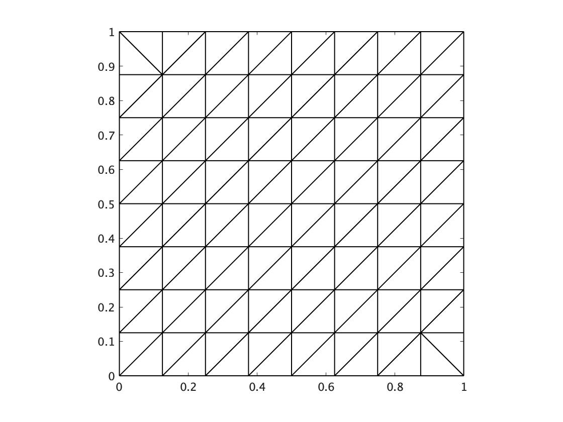
Figure 1: (I) Standard mesh

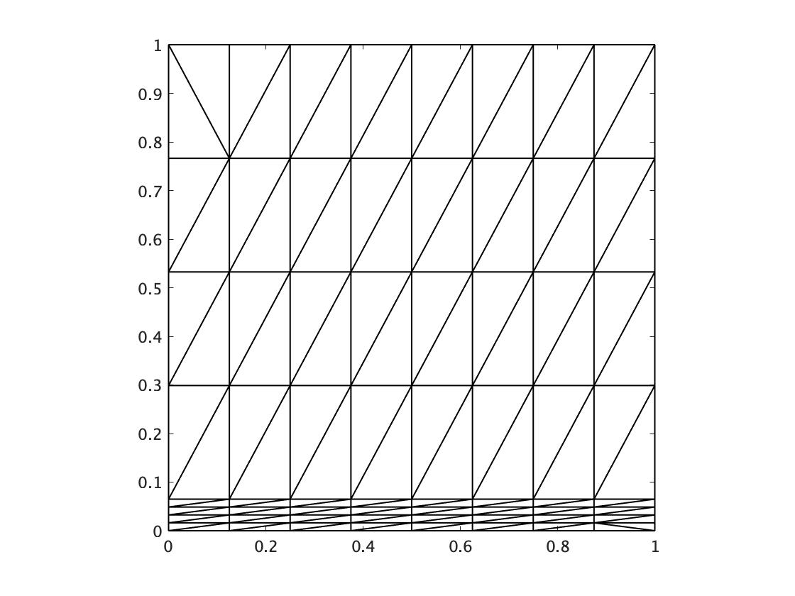
Figure 2: (II) Shishkin mesh, $\delta=\frac{1}{128}$

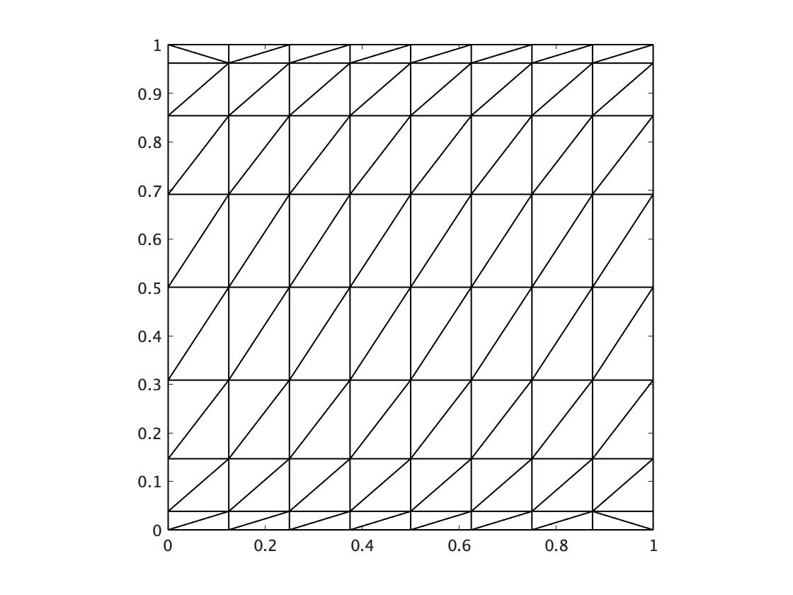
Figure 3: (III) Anisotropic mesh

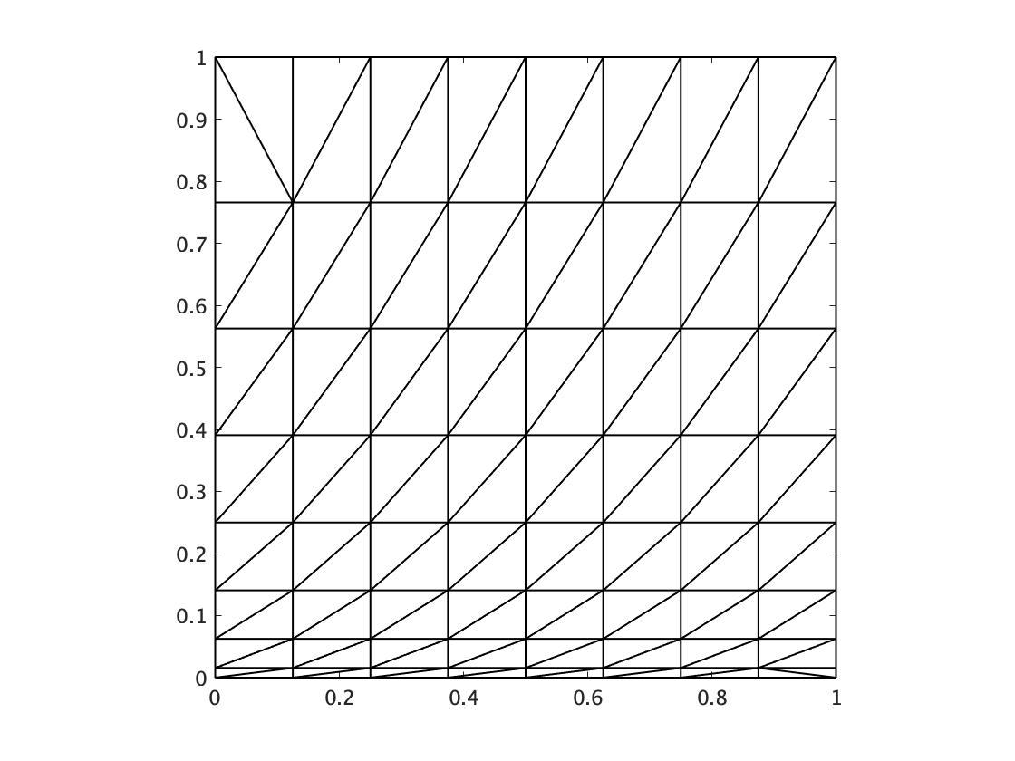
Figure 4: (IV) Anisotropic mesh

The shape-regularity condition is known: there exists a constant $\gamma_{1}\mathop{\textgreater}0$ such that

$$\displaystyle\rho_{T}\geq\gamma_{1}h_{T}\quad\forall\mathbb{T}_{h}\in\{\mathbb{T}_{h}\},\quad\forall T\in\mathbb{T}_{h},$$

and is equivalent to the following condition. There exists a constant $\gamma_{2}\mathop{\textgreater}0$ such that for any $\mathbb{T}_{h}\in\{\mathbb{T}_{h}\}$ and simplex $T\in\mathbb{T}_{h}$, we have

$$\displaystyle|T|_{2}\geq\gamma_{2}h_{T}^{2}.$$

A proof is provided in (BraKorKri08, , Theorem 1). The semiregularity mesh condition defined in (2.15) is equivalent to the maximum angle condition. The following parameters are computed.

$$\displaystyle\textit{MinAngle}:=\max_{T\in\mathbb{T}_{h}}\frac{|L_{3}|_{1}^{2}}{|T|_{2}},\quad\textit{MaxAngle}:=\max_{T\in\mathbb{T}_{h}}\frac{|L_{1}|_{1}|L_{2}|_{1}}{|T|_{2}},$$

where $L_{i}$, $i=1,2,3,$ denote the edges of the simplex $T\in\mathbb{T}_{h}$ with $|L_{1}|_{1}\leq|L_{2}|_{1}\leq|L_{3}|_{1}$.

Table 1: Mesh conditions

Mesh	$N$	MinAngle	MaxAngle
I	32	4.00000	2.00000
	64	4.00000	2.00000
II	32	9.66647	2.00000
	64	8.21423	2.00000
III	32	2.61132e+01	2.00000
	64	5.19640e+01	2.00000
IV	32	6.40625e+01	2.00000
	64	1.28031e+02	2.00000

Notably, a sequence with meshes (I) or (II) satisfies the shape-regularity condition, but a sequence with meshes (III), or (IV) does not satisfy the shape regularity condition.

We adopt the following schemes.

(1)

Scheme (3.1).

(2)

Hybrid dG (HdG) method with a penalty term. Let $k\in\mathbb{N}$. We define a discrete space as ${\Lambda}_{h}^{k}:=\{{\lambda}_{h}\in L^{2}(\mathcal{F}_{h})^{2}:\ {\lambda}_{h}|_{F}\in\mathbb{P}^{k}(F)^{2}\ \forall F\in\mathcal{F}_{h},\ {\lambda}_{h}|_{\partial\Omega}=0\}$. Find $(u_{h},\lambda_{h},p_{h})\in V_{dc,h}^{k}\times{\Lambda}_{h}^{k}\times P_{dc,h}^{k-1}$ such that

$$\displaystyle a_{h}^{HdG}(u_{h},\lambda_{h};v_{h},\mu_{h})+b_{h}^{HdG}(v_{h},\mu_{h};p_{h}) =\int_{\Omega}f\cdot v_{h}dx\quad\forall(v_{h},\mu_{h})\in V_{dc,h}^{k}\times{\Lambda}_{h}^{k},$$ (4.1a)

$$b_{h}^{HdG}(u_{h},\lambda_{h};q_{h})-10^{-10}\int_{\Omega}p_{h}q_{h}dx =0\quad\forall q_{h}\in P_{dc,h}^{k-1},$$ (4.1b)

where

$$\displaystyle a_{h}^{HdG}(u_{h},\lambda_{h};v_{h},\mu_{h}) :=\int_{\Omega}\nabla_{h}u_{h}:\nabla_{h}v_{h}dx$$

$$+\sum_{T\in\mathbb{T}_{h}}\sum_{F\in\mathcal{F}_{T}}\frac{{\eta}}{h_{F}}\int_{F}(\lambda_{h}-u_{h})\cdot(\mu_{h}-v_{h})ds$$

$$+\sum_{T\in\mathbb{T}_{h}}\int_{\partial T}\left(\nabla_{h}u_{h}n_{F}\cdot(\mu_{h}-v_{h})+(\lambda_{h}-u_{h})\cdot\nabla_{h}v_{h}n_{F}\right)ds,$$

$$b_{h}^{HdG}(v_{h},\mu_{h};q_{h}) :=-\int_{\Omega}\mathop{\mathrm{div}_{h}}v_{h}q_{h}dx-\sum_{T\in\mathbb{T}_{h}}\int_{\partial T}(\mu_{h}-v_{h})\cdot n_{F}q_{h}ds,$$

for any $(u_{h},\lambda_{h})\in V_{dc,h}^{k}\times{\Lambda}_{h}^{k}$, $(v_{h},\mu_{h})\in V_{dc,h}^{k}\times{\Lambda}_{h}^{k}$, and $q_{h}\in P_{dc,h}^{k-1}$. Here, ${\eta}$ is a positive real number.

(3)

Conforming finite element method with a penalty parameter. Let $k\in\mathbb{N}$. We define discrete spaces as $P_{c,h}^{k}:=\{p_{h}\in H^{1}(\Omega);\ p_{h}|_{T}\in\mathbb{P}^{k}(T)\ \forall T\in\mathbb{T}_{h}\}$, and $V_{c,h}^{2}:=(P_{c,h}^{2}\cap H_{0}^{1}(\Omega))^{2}$. Find $(u_{h},p_{h})\in V_{c,h}^{2}\times P_{c,h}^{1}$ such that

$$\displaystyle a_{h}^{c}(u_{h},v_{h})+b_{h}^{c}(v_{h},p_{h}) =\int_{\Omega}f\cdot v_{h}dx\quad\forall v_{h}\in V_{c,h}^{2},$$ (4.2a)

$$b_{h}^{c}(u_{h},q_{h})-10^{-10}\int_{\Omega}p_{h}q_{h}dx =0\quad\forall q_{h}\in P_{c,h}^{1},$$ (4.2b)

where

$$\displaystyle a_{h}^{c}(u_{h},v_{h}) :=\int_{\Omega}\nabla u_{h}:\nabla v_{h}dx,\quad b_{h}^{c}(v_{h},q_{h}):=-\int_{\Omega}\mathop{\mathrm{div}}v_{h}q_{h}dx,$$

for any $u_{h}\in V_{c,h}^{2}$, $v_{h}\in V_{c,h}^{2}$, and $q_{h}\in P_{c,h}^{1}$.

Remark 6

The original HdG method by EggWal13 is as follows. Find $(u_{h},\lambda_{h},p_{h})\in V_{h}^{k}\times{\Lambda}_{h}^{k}\times Q_{h}^{k-1}$ such that

$$\displaystyle a_{h}^{HdG}(u_{h},\lambda_{h};v_{h},\mu_{h})+b_{h}^{HdG}(v_{h},\mu_{h};p_{h}) =\int_{\Omega}f\cdot v_{h}dx\quad\forall(v_{h},\mu_{h})\in V_{h}^{k}\times{\Lambda}_{h}^{k},$$ (4.3a)

$$b_{h}^{HdG}(u_{h},\lambda_{h};q_{h}) =0\quad\forall q_{h}\in Q_{h}^{k-1},$$ (4.3b)

where the terms $a_{h}^{HdG}$ and $b_{h}^{HdG}$ are as defined above.

If an exact solution $u$ is known, the error $e_{h}:=u-u_{h}$ and $e_{h/2}:=u-u_{h/2}$ are computed numerically for two mesh sizes $h$ and $h/2$. The convergence indicator $r$ is defined by

$$\displaystyle r=\frac{1}{\log(2)}\log\left(\frac{\|e_{h}\|_{X}}{\|e_{h/2}\|_{X}}\right).$$

We compute the convergence order with respect to norms defined by

$$\displaystyle E_{u_{h}}^{(\text{Mesh No.})} :=\frac{|u-u_{h}|_{V_{dc,h}^{CR}}}{|u|_{H^{1}(\Omega)^{2}}}\quad\text{for scheme (1)},$$

$$E_{u_{h}}^{(\text{Mesh No.})} :=\frac{|u-u_{h}|_{H^{1}(\mathbb{T}_{h})^{2}}}{|u|_{H^{1}(\Omega)^{2}}}$$

$$\quad\quad\text{for schemes (2), (3), and the WBCR method},$$

$$\quad E_{u_{h},L^{2}}^{(\text{Mesh No.})} :=\frac{\|u-u_{h}\|_{L^{2}(\Omega)^{2}}}{\|u\|_{L^{2}(\Omega)^{2}}},\quad E_{p_{h}}^{(\text{Mesh No.})}:=\frac{\|p-p_{h}\|_{L^{2}(\Omega)}}{\|p\|_{L^{2}(\Omega)}}.$$

For the computation of scheme (1), we used the CG method without preconditioners, and the quadrature of the five order for computation of the right-hand side in (3.1a), see (ErnGue21b, , p. 85, Table 30.1). For the computation of the schemes (2), and (3), we used the FreeFEM software tool HecPioMorHyaOht12 ; Hec based on code provided in the prior work OikKik17 and used UMFPACK.

Table 2: Scheme (1)

Mesh	$N$	$E_{u_{h}}^{(\text{Mesh No.})}$	$r$	$E_{u_{h},L^{2}}^{(\text{Mesh No.})}$	$r$	$E_{p_{h}}^{(\text{Mesh No.})}$	$r$
I	32	8.10569e-01		2.12630e-01		3.61598e-02
	64	4.08981e-01	0.99	5.42357e-02	1.97	1.35562e-02	1.42
II	32	1.15924		4.33629e-01		6.52059e-02
	64	5.79411e-01	1.00	1.08800e-01	1.99	2.22654e-02	1.55
III	32	1.05163		3.60039e-01		5.24322e-02
	64	5.34097e-01	0.98	9.31283e-02	1.95	1.76734e-02	1.57
IV	32	1.23942		4.97459e-01		7.17788e-02
	64	6.36438e-01	0.96	1.31655e-01	1.92	2.44549e-02	1.55

Table 3: Scheme (2) with $k=1$

Mesh	$N$	${\eta}$	$E_{u_{h}}^{(\text{Mesh No.})}$	$r$	$E_{u_{h},L^{2}}^{(\text{Mesh No.})}$	$r$	$E_{p_{h}}^{(\text{Mesh No.})}$	$r$
I	32	20	7.65762e-02		6.54741e-03		2.35152e-02
	64	20	3.74884e-02	1.03	1.60004e-03	2.03	1.14994e-02	1.03
II	32	30	1.08934e-01		1.27498e-02		3.78265e-02
	64	30	4.50132e-02	1.28	3.03009e-03	2.07	1.84420e-02	1.04
III	32	40	8.22514e-02		1.01627e-02		2.92376e-02
	64	40	3.88132e-02	1.08	2.50863e-03	2.02	1.44096e-02	1.02
IV	32	40	9.87191e-02		1.34999e-02		3.86220e-02
	64	40	4.60525e-02	1.10	3.34145e-03	2.01	1.90213e-02	1.02

Table 4: Scheme (2) with $k=2$

Mesh	$N$	${\eta}$	$E_{u_{h}}^{(\text{Mesh No.})}$	$r$	$E_{u_{h},L^{2}}^{(\text{Mesh No.})}$	$r$	$E_{p_{h}}^{(\text{Mesh No.})}$	$r$
I	32	20	2.66367e-03		5.34649e-05		1.61446e-04
	64	20	6.65586e-04	2.00	6.72505e-06	2.99	4.03072e-05	2.00
II	32	20	7.45375e-03		1.79222e-04		3.96913e-04
	64	40	1.00195e-03	2.90	1.98821e-05	3.17	1.01078e-04	1.97
III	32	20	6.37078e-03		9.19734e-05		2.59598e-04
	64	40	7.54222e-04	3.08	1.06225e-05	3.11	7.90454e-05	1.72
IV	32	30	5.47512e-03		1.47191e-04		3.58253e-04
	64	60	1.11295e-03	2.30	1.95215e-05	2.91	1.44366e-04	1.31

Table 5: Scheme (3)

Mesh	$N$	$E_{u_{h}}^{(\text{Mesh No.})}$	$r$	$E_{u_{h},L^{2}}^{(\text{Mesh No.})}$	$r$	$E_{p_{h}}^{(\text{Mesh No.})}$	$r$
I	32	2.86851e-03		8.51503e-05		2.44204e-04
	64	7.18451e-04	2.00	1.06518e-05	3.00	6.09198e-05	2.00
II	32	5.11492e-03		2.31144e-04		5.25401e-04
	64	1.19256e-03	2.10	2.66944e-05	3.11	1.10624e-04	2.25
III	32	3.35828e-03		1.19972e-04		3.56077e-04
	64	8.41989e-04	2.00	1.50243e-05	3.00	8.89802e-05	2.00
IV	32	4.60495e-03		2.02053e-04		4.35519e-04
	64	1.16069e-03	1.99	2.52328e-05	3.00	1.08824e-04	2.00

The tables 2, 3, and 4 imply that the inf-sup condition is satisfied on anisotropic meshes. However, to the best of our knowledge, a theoretical analysis of the HdG method on anisotropic meshes has not been considered in the relevant literature. Furthermore, one needs to tune up the parameter $\eta$. The table 5 also implies that the inf-sup condition is satisfied on anisotropic meshes. The inf-sup condition in two-dimensional cases is proven in the previous work BarWac19 .

4.2 Penalty parameters

One disadvantage of the WOPSIP method is that it increases the number of conditions. In particular, the penalty parameter $\kappa_{F}$ increases as $h\to 0$. On the mesh (II), we compute the following qualities (Table 6).

$$\tau_{\max}^{(f)}:=\max_{F\in\mathcal{F}_{h}^{i}}\frac{1}{h_{F}},\quad\tau_{\max}^{(ave)}:=\max_{F\in\mathcal{F}_{h}^{i}}\frac{1}{4}\left(\frac{1}{{\ell_{T_{1},F}}}+\frac{1}{{\ell_{T_{2},F}}}\right),$$

$$\tau_{\max}^{(dg)}:=\max_{F\in\mathcal{F}_{h}^{i}}\frac{2}{\left(\sqrt{\ell_{T_{1},F}}+\sqrt{\ell_{T_{2},F}}\right)^{2}},\quad\tau_{\max}^{(wop)}:=\max_{F\in\mathcal{F}_{h}^{i}}\frac{2}{h^{2}\left(\sqrt{\ell_{T_{1},F}}+\sqrt{\ell_{T_{2},F}}\right)^{2}}$$

Table 6: Comparison of penalty parameters: Mesh (II): $\delta=\frac{1}{1024}$

$N$	$1/h$	$\tau_{\max}^{(f)}$	$\tau_{\max}^{(ave)}$	$\tau_{\max}^{(dg)}$	$\tau_{\max}^{(wop)}$
16	7.2179e+00	7.3866e+02	3.6942e+02	3.6942e+02	1.9246e+04
32	1.4467e+01	1.1819e+03	5.9114e+02	5.9114e+02	1.2373e+05
64	2.8998e+01	1.9698e+03	9.8540e+02	9.8540e+02	8.2860e+05
128	5.8123e+01	3.3767e+03	1.6896e+03	1.6896e+03	5.7079e+06
256	1.1650e+02	5.9093e+03	2.9574e+03	2.9574e+03	4.0139e+07

Table 6 shows that the penalty parameter of the WOPSIP method is considerably larger than the others. The problem of the ill-conditioning on anisotropic meshes is left for future research. The improvement of the ill-conditioning for the Poisson equation is stated in BreOweSun08 .

4.3 Comparison of the penalty parameters

Numerical calculations for the problem in Section 4.1 were performed using the parameter $\kappa_{F*}$ instead of the parameter $\kappa_{F}$ for scheme (3.1). The convergence order was computed with respect to the norms defined by

$$\displaystyle E_{h}^{(\text{Mesh No.})} :=\frac{|u-u_{h}|_{V_{dc,h}^{CR}}+\|p-p_{h}\|_{L^{2}(\Omega)}}{|u|_{H^{1}(\Omega)^{2}}+\|p\|_{L^{2}(\Omega)}}.$$

Table 7 presents the numerical results obtained using Mesh (I). The case that uses parameter $\kappa_{F*}$ is unlikely to converge.

Table 7: WOPSIP method with $\kappa_{F}$, $\kappa_{F*}$

$N$	$\#Np$	$h$	$E_{h}^{(I)}(\kappa_{F})$	$r$	$E_{h}^{(I)}(\kappa_{F*})$	$r$
16	3,584	8.84e-02	2.81448e-01		1.81628
32	14,336	4.42e-02	1.28586e-01	1.13	1.81324	-
64	57,344	2.21e-02	6.07505e-02	1.08	1.81236	-
128	229,376	1.10e-02	2.97281e-02	1.03	1.81213	-
256	917,504	5.52e-03	1.47711e-02	1.01	1.81207	-

4.4 Comparison with the well-balanced CR method

We set $\varphi(x_{1},x_{2}):=x_{1}^{2}(x_{1}-1)^{2}x_{2}^{2}(x_{2}-1)^{2}\exp\left(-\frac{x_{2}}{\eta}\right)$ with $\eta:=\sqrt{\delta}$ and $\delta\in\left\{\frac{1}{64},\frac{1}{128},\frac{1}{256}\right\}$. The function $f$ of the Stokes equation (2.1) with $\nu=1$ is given so that the exact solution is

$$\displaystyle\begin{pmatrix}u_{1}\\ u_{2}\end{pmatrix}=\begin{pmatrix}\frac{\partial\varphi}{\partial x_{2}}\\ -\frac{\partial\varphi}{\partial x_{1}}\end{pmatrix},\quad p=x_{1}^{2}(x_{1}-1)^{2}\exp\left(-\frac{x_{2}}{\delta}\right)-\frac{\delta}{30}+\frac{\delta}{30}\exp\left(-\frac{1}{\delta}\right).$$

Note that $\int_{\Omega}pdx\approx 0$. See Fig. 5.

Remark 7

Through a simple calculation,

$$\displaystyle\frac{\partial^{2}u_{1}}{\partial x_{2}^{2}} =\left(-\frac{1}{\eta^{3}}x_{1}^{2}(x_{1}-1)^{2}x_{2}^{2}(x_{2}-1)^{2}+C_{1}\left(x_{1},x_{2},\eta\right)\right)\exp\left(-\frac{x_{2}}{\eta}\right),$$

$$\frac{\partial^{2}u_{2}}{\partial x_{2}^{2}} =-\frac{2}{\eta^{2}}\left(x_{1}(x_{1}-1)^{2}+x_{1}^{2}(x_{1}-1)\right)x_{2}^{2}(x_{2}-1)^{2}\exp\left(-\frac{x_{2}}{\eta}\right)$$

$$\quad+C_{2}\left(x_{1},x_{2},\eta\right)\exp\left(-\frac{x_{2}}{\eta}\right),$$

$$\frac{\partial p}{\partial x_{2}} =-\frac{1}{\delta}x_{1}^{2}(x_{1}-1)^{2}\exp\left(-\frac{x_{2}}{\delta}\right),$$

where $C_{1}\left(x_{1},x_{2},\eta\right)$ and $C_{2}\left(x_{1},x_{2},\eta\right)$ are functions. In this numerical experiment, we set $\eta=\sqrt{\delta}$.

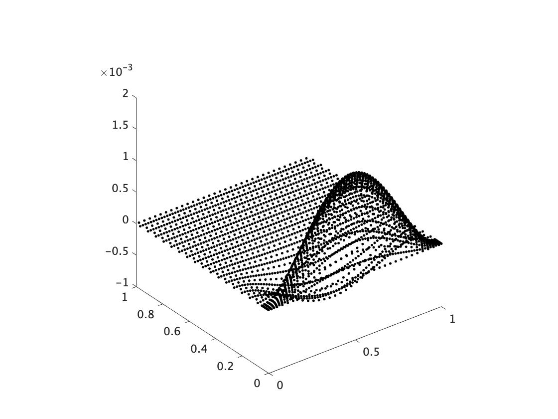
(a) Plot of $u_{1}$

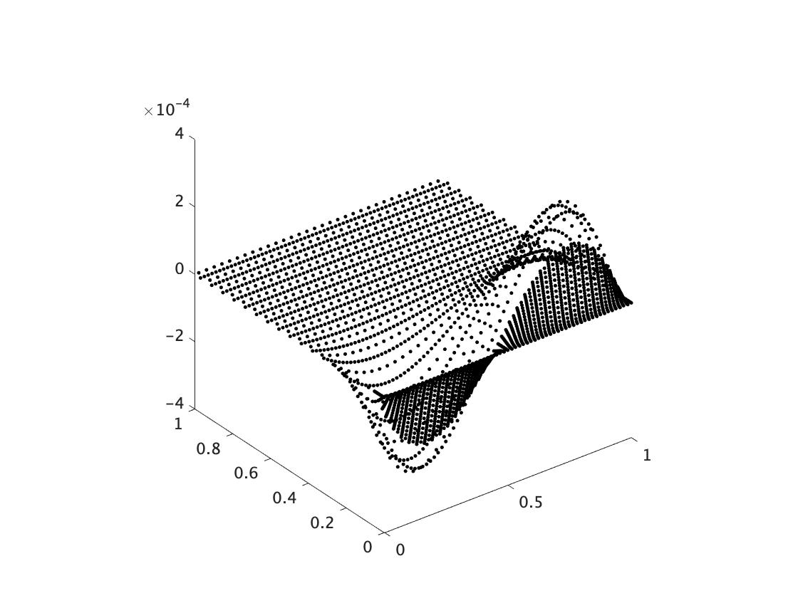
(b) Plot of $u_{2}$

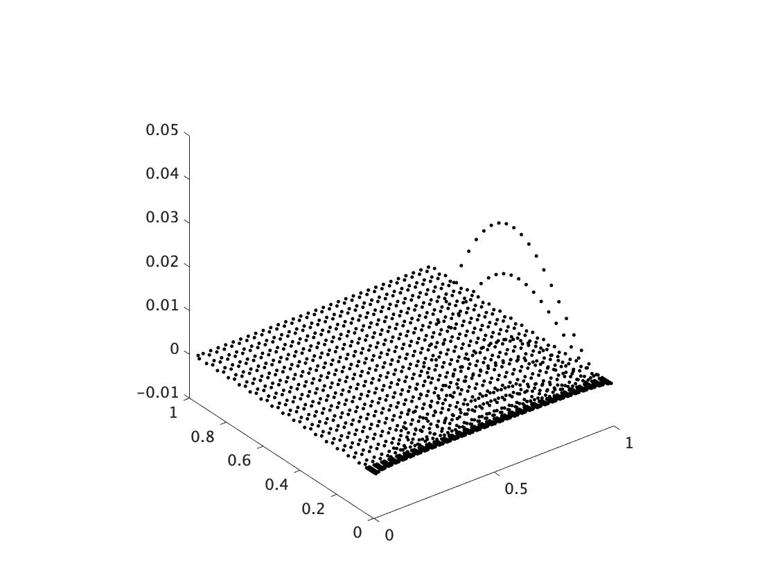
(c) Plot of $p$

Figure 5: Mesh (II) Plot of the exact solution, $\eta=\frac{1}{16}$, $\delta=\frac{1}{256}$

In the computation, the following schemes were used:

(1)

Scheme (3.1) (WOPSIP method).

(4)

Well-balanced CR (WBCR) method (Lin14 ). We define the classical RT finite element space as

$$\displaystyle V_{c,h}^{RT} :=\{v_{h}\in V_{dc,h}^{RT}:\ [\![v_{h}\cdot n]\!]_{F}=0,\ \forall F\in\mathcal{F}_{h}\}.$$

Let $\mathcal{I}_{h}^{RTc}:V_{h0}^{CR}\to V_{c,h}^{RT}$ be a classical RT interpolation operator. Find $(u_{h},p_{h})\in V_{h0}^{CR}\times Q_{h}^{0}$ such that

$$\displaystyle a_{h}^{CR}(u_{h},v_{h})+b_{h}^{CR}(v_{h},p_{h}) =\int_{\Omega}f\cdot\mathcal{I}_{h}^{RTc}v_{h}dx\quad\forall v_{h}\in V_{h0}^{CR},$$ (4.4a)

$$b_{h}^{CR}(u_{h},q_{h}) =0\quad\forall q_{h}\in Q_{h}^{0},$$ (4.4b)

where

$$\displaystyle a_{h}^{CR}(u_{h},v_{h}) :=\sum_{i=1}^{d}\int_{\Omega}\nabla_{h}u_{h,i}\cdot\nabla_{h}v_{h,i}dx,$$

$$b_{h}^{CR}(v_{h},q_{h}) :=-\int_{\Omega}\mathop{\mathrm{div}_{h}}v_{h}q_{h}dx,$$

for $u_{h},v_{h}\in V_{h0}^{CR}$ and $q_{h}\in Q_{h}^{0}$. Recall that space $V_{h0}^{CR}$ was defined in Remark 5.

Let $N\in\{16,32,64,128,256\}$ be the division number for each side of the bottom and height edges of $\Omega$. We consider meshes (I) and (II) with $\delta\in\left\{\frac{1}{64},\frac{1}{128},\frac{1}{256}\right\}$. The notation $\#Np$ denotes the number of nodal points on $V_{dc,h}^{CR}\times Q_{h}^{0}$ or $V_{h0}^{CR}\times Q_{h}^{0}$ including nodal points on the boundary. We further use the CG method without preconditioners and the quadrature of the five orders for the computation of the right-hand side in (3.1a) and (4.4a).

Table 8: Mesh (I) WOPSIP method, $\eta=\frac{1}{8}$, $\delta=\frac{1}{64}$

$N$	$\#Np$	$h$	$E_{u_{h}}^{(I)}$	$r$	$E_{p_{h}}^{(I)}$	$r$
16	3,584	8.84e-02	6.84774e-01		8.83176e-01
32	14,336	4.42e-02	3.81183e-01	0.85	5.23969e-01	0.75
64	57,344	2.21e-02	1.98511e-01	0.94	2.72238e-01	0.94
128	229,376	1.10e-02	1.00464e-01	0.98	1.37158e-01	0.99
256	917,504	5.52e-03	5.03923e-02	1.00	6.86957e-02	1.00

Table 9: Mesh (II) WOPSIP method, $\eta=\frac{1}{8}$, $\delta=\frac{1}{64}$

$N$	$\#Np$	$h$	$E_{u_{h}}^{(I)}$	$r$	$E_{p_{h}}^{(I)}$	$r$
16	3,584	8.84e-02	4.99659e-01		6.39849e-01
32	14,336	4.42e-02	2.66696e-01	0.91	3.41427e-01	0.91
64	57,344	2.21e-02	1.42234e-01	0.91	1.83575e-01	0.90
128	229,376	1.10e-02	7.58869e-02	0.91	9.90536e-02	0.89
256	917,504	5.52e-03	4.04865e-02	0.91	5.34495e-02	0.89

Table 10: Mesh (I) WOPSIP method, $\eta=\frac{1}{8\sqrt{2}}$, $\delta=\frac{1}{128}$

$N$	$\#Np$	$h$	$E_{u_{h}}^{(I)}$	$r$	$E_{p_{h}}^{(I)}$	$r$
16	3,584	8.84e-02	8.23155e-01		1.05497
32	14,336	4.42e-02	4.89480e-01	0.75	8.08138e-01	0.38
64	57,344	2.21e-02	2.70311e-01	0.86	4.90630e-01	0.72
128	229,376	1.10e-02	1.41134e-01	0.94	2.57758e-01	0.93
256	917,504	5.52e-03	7.15209e-02	0.98	1.30291e-01	0.98

Table 11: Mesh (II) WOPSIP method, $\eta=\frac{1}{8\sqrt{2}}$, $\delta=\frac{1}{128}$

$N$	$\#Np$	$h$	$E_{u_{h}}^{(II)}$	$r$	$E_{p_{h}}^{(II)}$	$r$
16	3,584	1.30e-01	5.97426e-01		9.36325e-01
32	14,336	6.39e-02	3.13359e-01	0.93	4.83980e-01	0.95
64	57,344	3.14e-02	1.62259e-01	0.95	2.51145e-01	0.95
128	229,376	1.54e-02	8.35607e-02	0.96	1.30872e-01	0.94
256	917,504	7.55e-03	4.30401e-02	0.96	6.83930e-02	0.94

Table 12: Mesh (I) WOPSIP method, $\eta=\frac{1}{16}$, $\delta=\frac{1}{256}$

$N$	$\#Np$	$h$	$E_{u_{h}}^{(I)}$	$r$	$E_{p_{h}}^{(I)}$	$r$
16	3,584	8.84e-02	9.50427e-01		1.12990
32	14,336	4.42e-02	6.04935e-01	0.65	9.94423e-01	0.18
64	57,344	2.21e-02	3.49110e-01	0.79	7.71574e-01	0.37
128	229,376	1.10e-02	1.94504e-01	0.84	4.72726e-01	0.71
256	917,504	5.52e-03	1.02293e-01	0.93	2.49118e-01	0.92

Table 13: Mesh (II) WOPSIP method, $\eta=\frac{1}{16}$, $\delta=\frac{1}{256}$

$N$	$\#Np$	$h$	$E_{u_{h}}^{(II)}$	$r$	$E_{p_{h}}^{(II)}$	$r$
16	3,584	1.35e-01	7.89295e-01		1.46492
32	14,336	6.69e-02	4.10272e-01	0.94	7.48414e-01	0.97
64	57,344	3.31e-02	2.11273e-01	0.96	3.81425e-01	0.97
128	229,376	1.64e-02	1.07657e-01	0.97	1.94667e-01	0.97
256	917,504	8.13e-03	5.45969e-02	0.98	9.95082e-02	0.97

Table 14: Mesh (I) WBCR method, $\eta=\frac{1}{8}$, $\delta=\frac{1}{64}$

$N$	$\#Np$	$h$	$E_{u_{h}}^{(I)}$	$r$	$E_{p_{h}}^{(I)}$	$r$
16	3,584	8.84e-02	9.81333e-01		1.38484
32	14,336	4.42e-02	5.23575e-01	0.91	6.14362e-01	1.17
64	57,344	2.21e-02	2.65825e-01	0.98	2.84631e-01	1.11
128	229,376	1.10e-02	1.33413e-01	0.99	1.38739e-01	1.04
256	917,504	5.52e-03	6.67689e-02	1.00	6.88943e-02	1.01

Table 15: Mesh (II) WBCR method, $\eta=\frac{1}{8}$, $\delta=\frac{1}{64}$

$N$	$\#Np$	$h$	$E_{u_{h}}^{(I)}$	$r$	$E_{p_{h}}^{(I)}$	$r$
16	3,584	8.84e-02	7.58108e-01		7.22029e-01
32	14,336	4.42e-02	3.93515e-01	0.95	3.58341e-01	1.01
64	57,344	2.21e-02	2.04706e-01	0.94	1.86657e-01	0.94
128	229,376	1.10e-02	1.06968e-01	0.94	9.95828e-02	0.91
256	917,504	5.52e-03	5.60719e-02	0.93	5.35364e-02	0.90

Table 16: Mesh (I) WBCR method, $\eta=\frac{1}{8\sqrt{2}}$, $\delta=\frac{1}{128}$

$N$	$\#Np$	$h$	$E_{u_{h}}^{(I)}$	$r$	$E_{p_{h}}^{(I)}$	$r$
16	3,584	8.84e-02	1.26704		1.75263
32	14,336	4.42e-02	7.05425e-01	0.84	9.54909e-01	0.88
64	57,344	2.21e-02	3.61245e-01	0.97	5.12135e-01	0.90
128	229,376	1.10e-02	1.81656e-01	0.99	2.60500e-01	0.98
256	917,504	5.52e-03	9.09561e-02	1.00	1.30634e-01	1.00

Table 17: Mesh (II) WBCR method, $\eta=\frac{1}{8\sqrt{2}}$, $\delta=\frac{1}{128}$

$N$	$\#Np$	$h$	$E_{u_{h}}^{(II)}$	$r$	$E_{p_{h}}^{(II)}$	$r$
16	3,584	1.30e-01	9.89743e-01		1.02200
32	14,336	6.39e-02	5.02759e-01	0.98	4.96331e-01	1.04
64	57,344	3.14e-02	2.53831e-01	0.99	2.53006e-01	0.97
128	229,376	1.54e-02	1.28052e-01	0.99	1.31165e-01	0.95
256	917,504	7.55e-03	6.47475e-02	0.98	6.84384e-02	0.94

Table 18: Mesh (I) WBCR method, $\eta=\frac{1}{16}$, $\delta=\frac{1}{256}$

$N$	$\#Np$	$h$	$E_{u_{h}}^{(I)}$	$r$	$E_{p_{h}}^{(I)}$	$r$
16	3,584	8.84e-02	1.56033		2.05430
32	14,336	4.42e-02	9.44351e-01	0.72	1.20348	0.77
64	57,344	2.21e-02	4.91889e-01	0.94	8.06744e-01	0.58
128	229,376	1.10e-02	2.48251e-01	0.99	4.77567e-01	0.76
256	917,504	5.52e-03	1.24408e-01	1.00	2.49727e-01	0.94

Table 19: Mesh (II) WBCR method, $\eta=\frac{1}{16}$, $\delta=\frac{1}{256}$

$N$	$\#Np$	$h$	$E_{u_{h}}^{(II)}$	$r$	$E_{p_{h}}^{(II)}$	$r$
16	3,584	1.35e-01	1.32981		1.78771
32	14,336	6.69e-02	6.72574e-01	0.98	7.85551e-01	1.19
64	57,344	3.31e-02	3.38546e-01	0.99	3.83474e-01	1.03
128	229,376	1.64e-02	1.69928e-01	0.99	1.93935e-01	0.98
256	917,504	8.13e-03	8.51702e-02	1.00	9.87999e-02	0.97

Tables 8 - 13 represent numerical results of the WOPSIP method for $\delta=\frac{1}{64},\frac{1}{128},\frac{1}{256}$, respectively. Tables 14 - 19 represent numerical results of the WBCR method for $\delta=\frac{1}{64},\frac{1}{128},\frac{1}{256}$, respectively. The WBCR method showed a trend similar to that of the WOPSIP method. We observe that the use of the Shishkin mesh (II) with the parameter $\tau=4\delta\ln(N)$ near the bottom is likely to achieve the optimal convergence order, whereas Tables 12 and 18 show that the mesh needs to be split sufficiently to obtain the optimum convergence order on the standard mesh (I). These demonstrate the effectiveness of the anisotropic meshes.
We illustrate approximate solutions for the boundary layer problem can be found below (Figure 6 - Figure 11) when Mesh (II), $N=32$ and $\delta=\frac{1}{64},\frac{1}{128},\frac{1}{256}$. Even from the perspective of approximate solutions, it can be observed that numerical oscillations are occurring in $u_{h,2}$ and $p_{h}$ in both methods. However, the oscillations of the WBCR method seem to be small. Furthermore, it can be observed that the oscillations do not spread throughout the domain. Numerical oscillations seem inevitable even if the Shishkin mesh is used. These results imply that other techniques may be needed to reduce unnatural plots near the boundary layer for approximate solutions in Navier–Stokes equations (e.g., (ErnGue04, , Section 3.5), RooStyTob08 ).

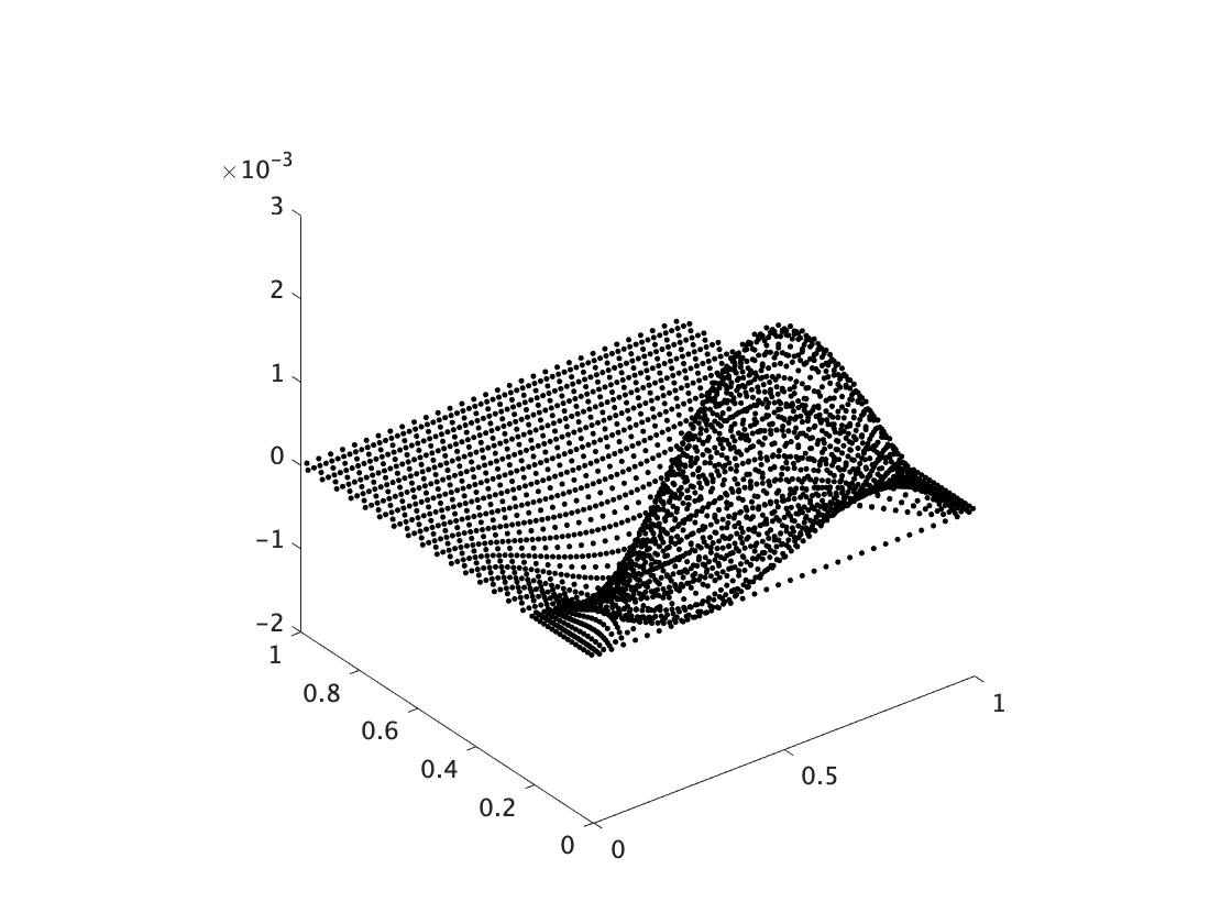
(a) Plot of $u_{h,1}$

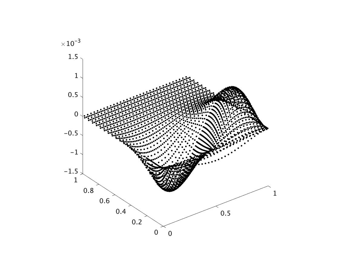
(b) Plot of $u_{h,2}$

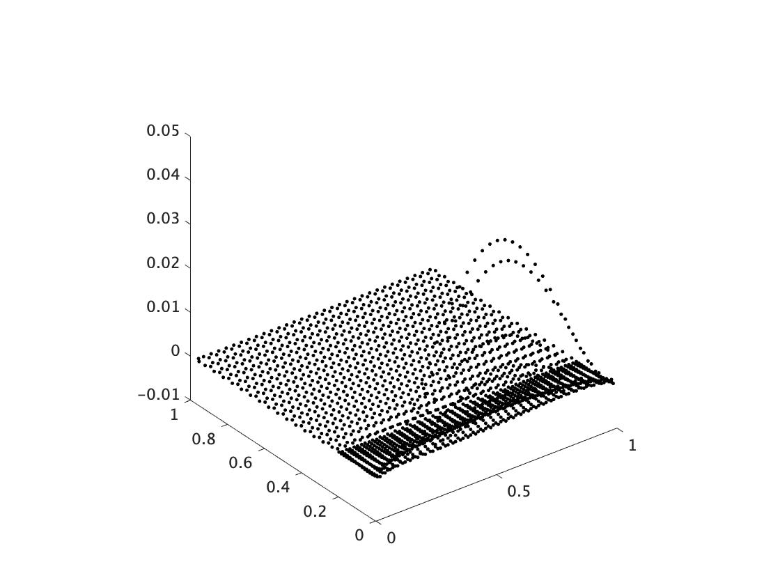
(c) Plot of $p_{h}$

Figure 6: Mesh (II) Plot of the WOPSIP solution, $\eta=\frac{1}{8}$, $\delta=\frac{1}{64}$

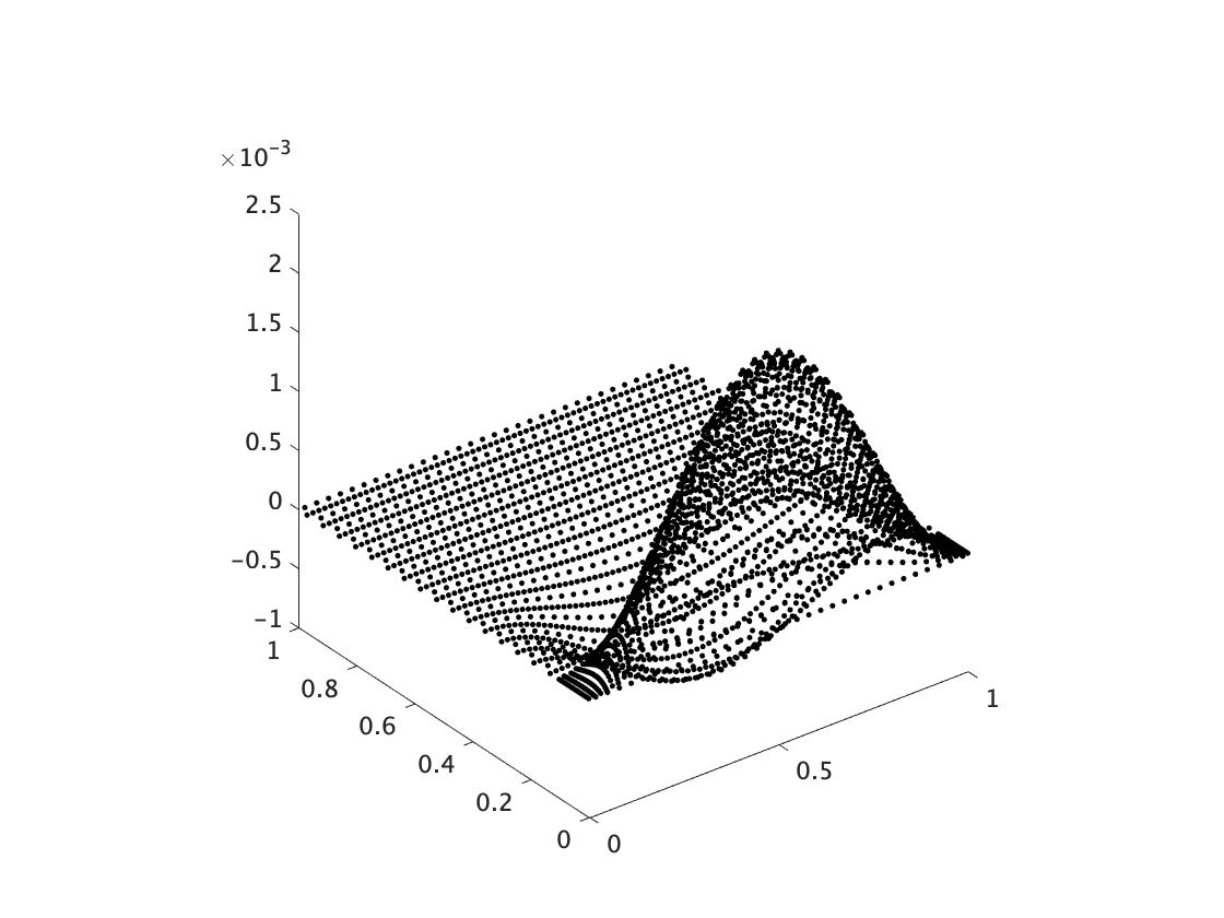
(a) Plot of $u_{h,1}$

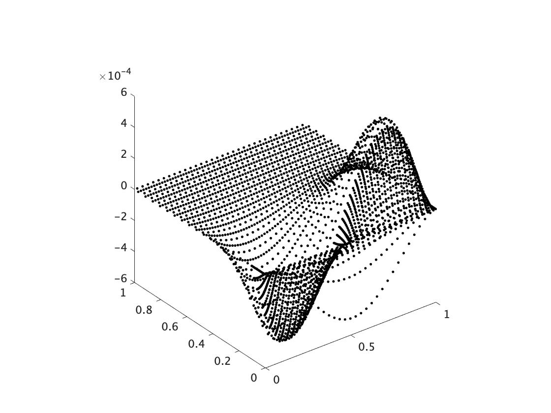
(b) Plot of $u_{h,2}$

(c) Plot of $p_{h}$

Figure 7: Mesh (II) Plot of the WOPSIP solution, $\eta=\frac{1}{8\sqrt{2}}$, $\delta=\frac{1}{128}$

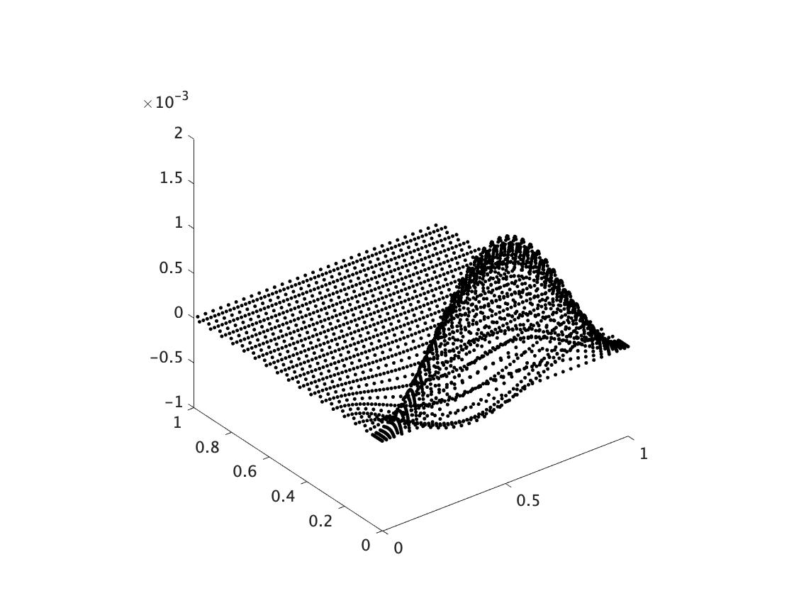
(a) Plot of $u_{h,1}$

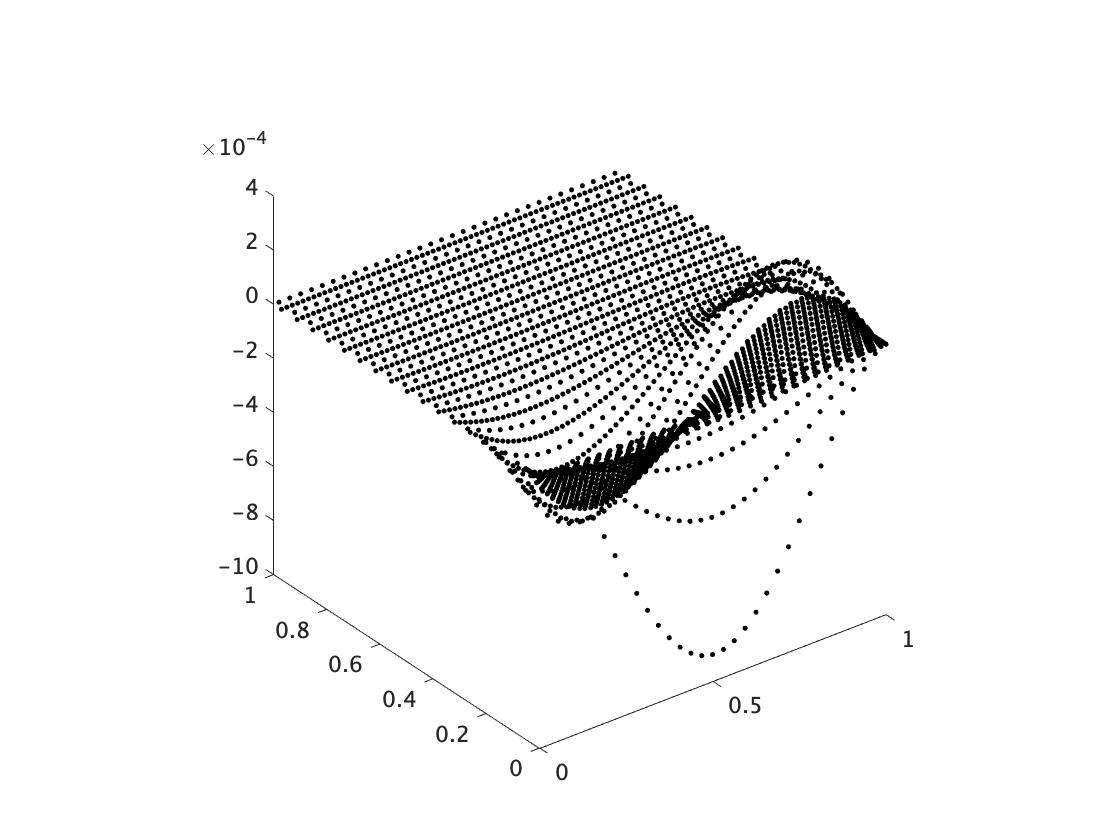
(b) Plot of $u_{h,2}$

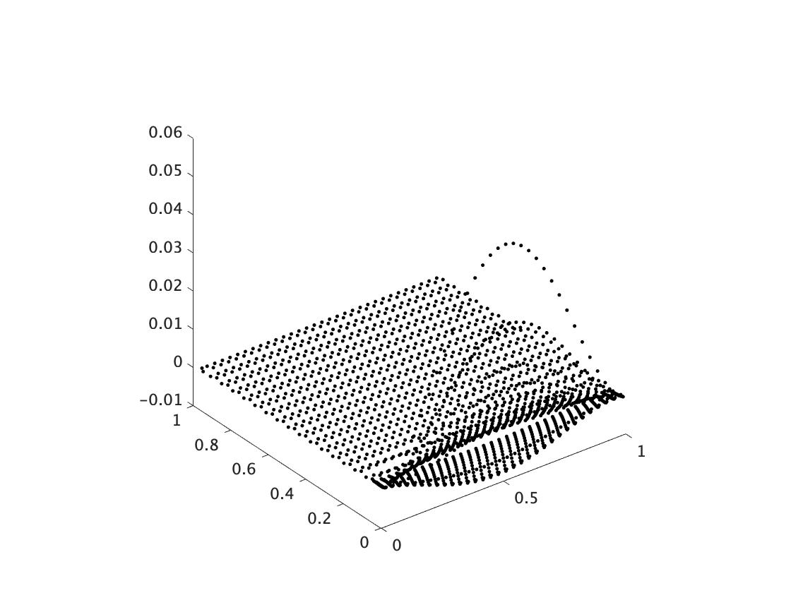
(c) Plot of $p_{h}$

Figure 8: Mesh (II) Plot of the WOPSIP solution, $\eta=\frac{1}{16}$, $\delta=\frac{1}{256}$

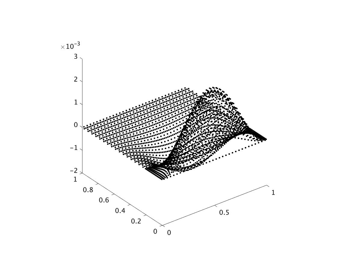
(a) Plot of $u_{h,1}$

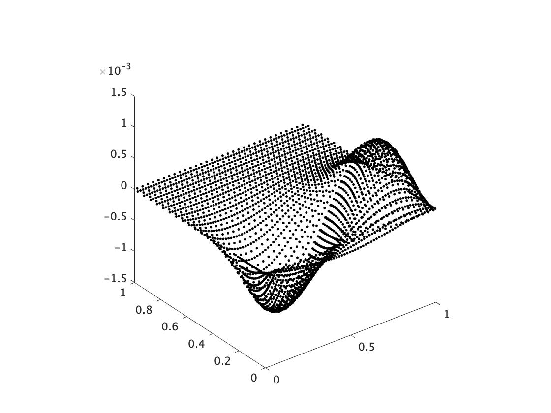
(b) Plot of $u_{h,2}$

(c) Plot of $p_{h}$

Figure 9: Mesh (II) Plot of the WBCR solution, $\eta=\frac{1}{8}$, $\delta=\frac{1}{64}$

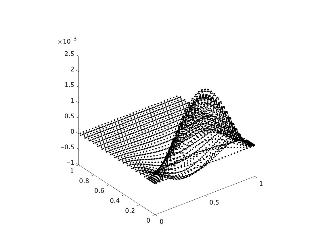
(a) Plot of $u_{h,1}$

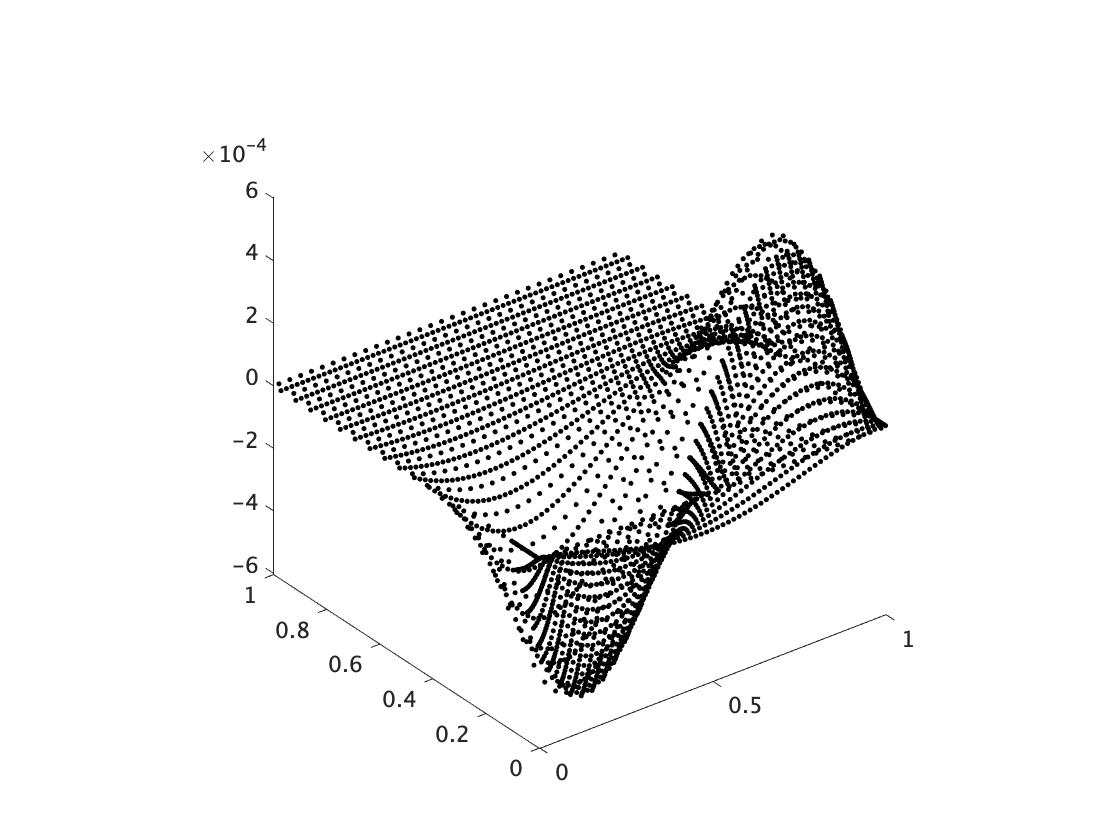
(b) Plot of $u_{h,2}$

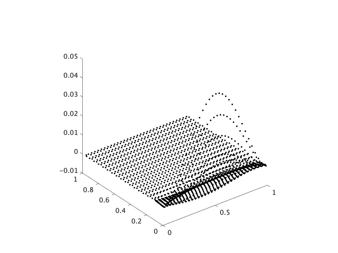
(c) Plot of $p_{h}$

Figure 10: Mesh (II) Plot of the WBCR solution, $\eta=\frac{1}{8\sqrt{2}}$, $\delta=\frac{1}{128}$

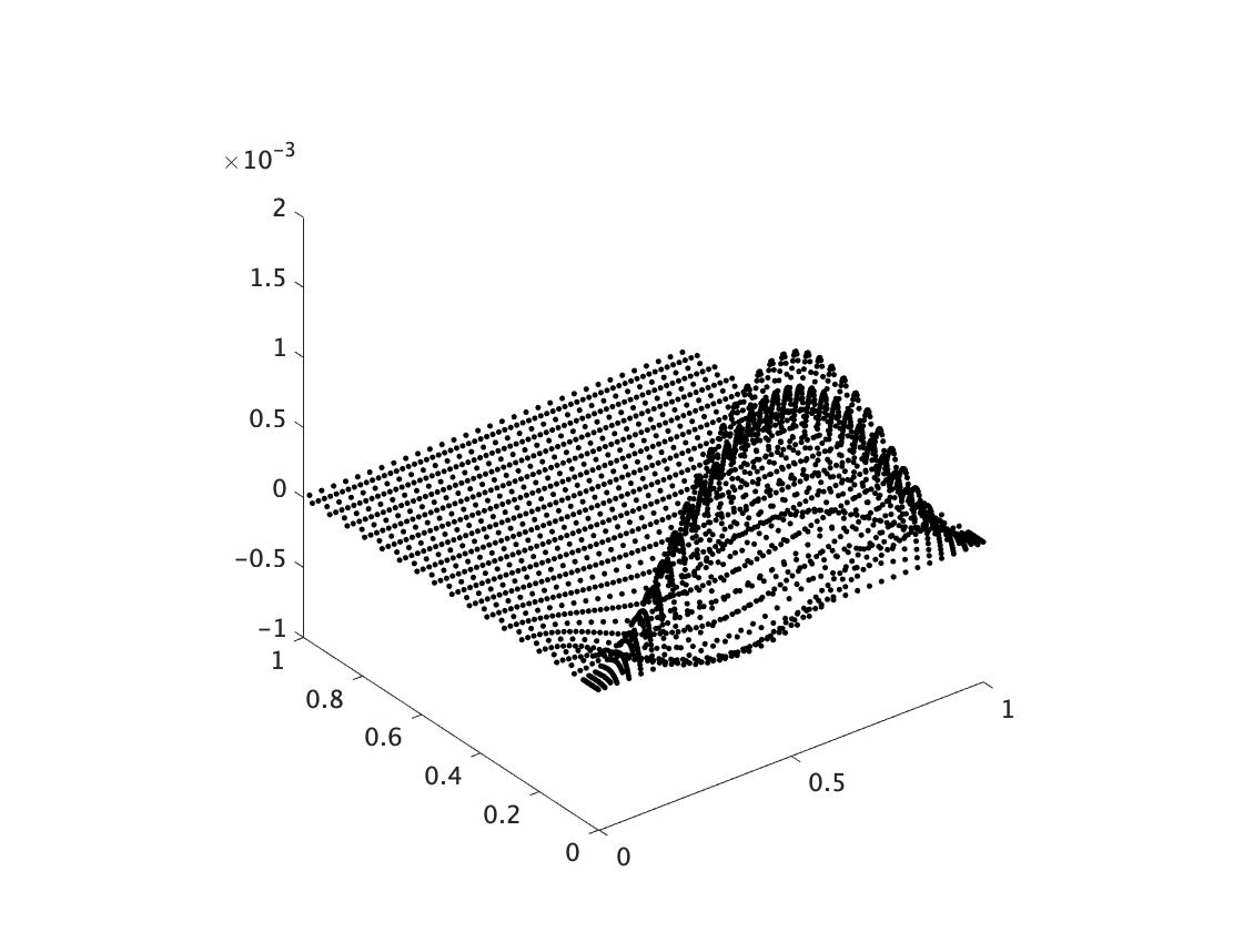
(a) Plot of $u_{h,1}$

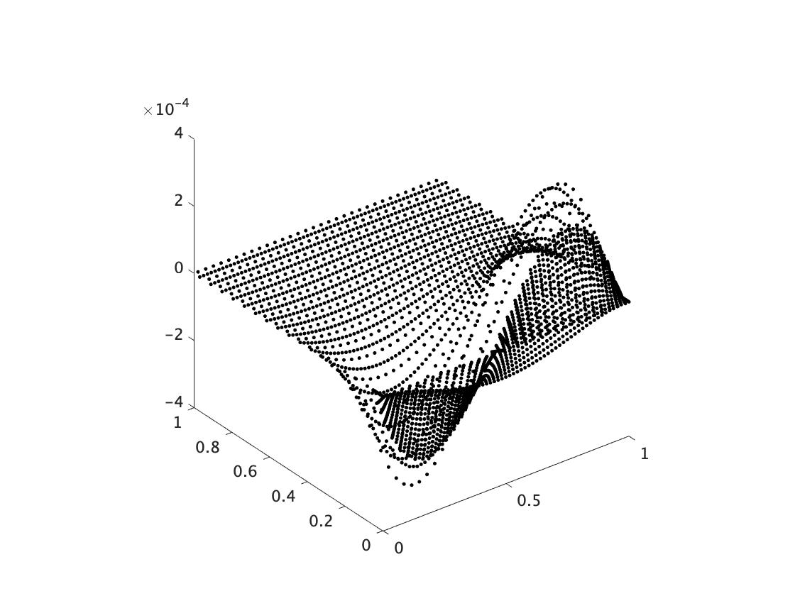
(b) Plot of $u_{h,2}$

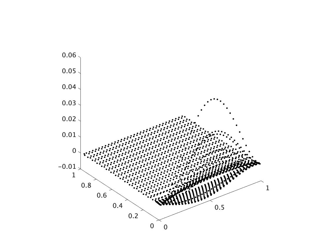
(c) Plot of $p_{h}$

Figure 11: Mesh (II) Plot of the WBCR solution, $\eta=\frac{1}{16}$, $\delta=\frac{1}{256}$

5 Concluding remarks

In conclusion, we identify several topics related to the results described in this work.

5.1 Discrete Poincaré and Sobolev inequalities

The discrete Poincaré and Sobolev inequalities play important roles in finite element analysis. However, to the best of our knowledge, the derivation of those inequalities remains an open question in nonconforming finite element methods on anisotropic meshes, although those inequalities are derived in PieErn12 on shape-regular meshes. In this article, we have derived the discrete Poincaré inequality by imposing that $\Omega$ is convex. Because we used the regularity of the solution of the dual problem, the convexity can be not violated in our method. In Bre03 , the discrete Poincaré inequalities for piecewise $H^{1}$ functions are proposed. However, the inverse, trace inequalities and the local quasi-uniformity for meshes under the shape-regular condition are used for the proof. Therefore, careful consideration of the results used in Bre03 may be necessary to remove the assumption that $\Omega$ is convex. For example, it may be necessary to assume the minimum angle condition for simplices within macro elements. We leave further investigation of this problem as a topic for future work.

5.2 Advantages of the WOPSIP method

The dG scheme based on the WOPSIP method has advantages on anisotropic mesh partitions. One key advantage of the WOPSIP method is that it does not require any penalty parameter tuning. The Stokes element proposed in (2.25) satisfies the inf-sup condition. Another advantage of the method is that the error analysis of the technique is studied on more general meshes (BreOweSun12 ; BreOweSun08 ; Bre15 ; BarBre14 ) than conformal meshes. This enables meshes with hanging nodes, whereas handling those meshes in the classical CR nonconforming finite element might be difficult. Here, we briefly treat the WOPSIP method on nonconforming meshes in our framework.

Let $d=2$. According to (Bre15, , Section 2.7), a nonconforming $\mathbb{T}_{h}$ on $\Omega$ is defined as satisfying the following condition:

• If an edge of $T\in\mathbb{T}_{h}$ contains hanging nodes, it is the union of the edges of other triangles in $\mathbb{T}_{h}$.

The definition of the set $\mathcal{F}_{h}^{i}$ in Section 2.3 is modified as follows: An (open) interior edge of a triangle in $\mathbb{T}_{h}$ belongs to $\mathcal{F}_{h}^{i}$ if and only if

(I)

it is the common edge of exactly two triangles, or

(II)

it contains a hanging node.

An excellent feature of the WOPSIP method for nonconforming is that the CR interpolation defined in (2.26) is unaffected by the hanging nodes; that is, the relations (3.16) and (3.24) remain valid. Therefore, if the relation (3.7) holds, then the error estimates in Theorem 3.7 may provide coverage as $h\to 0$ for nonconforming meshes. We leave further investigation of the hanging nodes for future work.

Data Availibility

Data supporting the findings of this study are available from the corresponding author upon request.

Conflict of interest

The authors declare no conflicts of interest associated with this manuscript.

References

• (1) Acosta, G., Apel, Th., Durán, R.G., Lombardi, A.L.: Error estimates for Raviart–Thomas interpolation of any order on anisotropic tetrahedra, Mathematics of Computation 80 No. 273, 141-163 (2010)
• (2) Acosta, G., Durán, R.G.: The maximum angle condition for mixed and nonconforming elements: Application to the Stokes equations, SIAM J. Numer. Anal 37, 18-36 (1999)
• (3) Apel Th, Nicaise S, Schöberl J: Crouzeix–Raviart type finite elements on anisotropic meshes. Numer Math 89, 193-223 (2001)
• (4) Andreas W. Stabilised mixed finite-element methods on anisotropic meshes. PhD thesis: University of Strathclyde (2015)
• (5) Apel, T. Anisotropic finite elements: local estimates and applications. Advances in Numerical Mathematics. Teubner & Stuttgart (1999)
• (6) Apel, T., Kempf V., Linke, A. and Merdon, C.. Non-conforming pressure-robust finite element method for Stokes equations on anisotropic meshes. IMA J. Numer. Anal., (2021)
• (7) Babu$\rm{\breve{s}}$ka, I. Aziz, A. K.: On the angle condition in finite element method. SIAM J. Numer. Anal. 13, 214-226 (1976)
• (8) Barker, A. T., Brenner, S. C.: A mixed finite element method for the Stokes equations based on a weakly overpenalized symmetric interior penalty approach. J. Sci. Comput. 58, 290-307 (2014)
• (9) Barrenechea, G. R., Wachtel, A.: The inflow stability of the lowest-order Taylor–Hood pair on affine anisotropic meshes. IMA J. Numer. Anal. 40, 2377-2398 (2019)
• (10) Boffi, D., Brezzi, F., Demkowicz, L.F., Durán, R.G., Falk, R.S., Fortin, M.: Mixed Finite Elements, Compatibility Conditions, and Applications: Lectures Given at the C.I.M.E. Summer School, Italy, 2006. Lunk Notes in Mathematics 1939 and Springer (2008)
• (11) Boffi, D., Brezzi, F., Fortin, M.: Mixed Finite Element Methods and Applications. Springer-Verlag, New York (2013).
• (12) Brandts, J., Korotov, S. & K$\rm{\check{r}}$í$\rm{\check{z}}$ek, M.: On the equivalence of regularity criteria for triangular and tetrahedral finite-element partitions. Comput. Math, Appl. 55, 2227–2233 (2008)
• (13) Brenner, S. C.: Poincaré–Friedrichs inequalities for piecewise $H^{1}$ functions. SIAM J. Numer. Anal. 41 (1), 306-324 (2003)
• (14) Brenner, S. C. Forty years of the Crouzeix–Raviart element. Numer. Methods Partial Differential Equations 31, 367-396 (2015)
• (15) Brenner, S. C., Owens, L., Sung, L. Y., A weakly over-penalised symmetric interior penalty method. Electron. Trans. Numer. Anal. 30, 107-127 (2008)
• (16) Brenner, S. C., Owens, L., Sung, L. Y.: Higher-order weakly overpenalized symmetric interior penalty methods. J. Comput. App. Math 236, 2883-2894 (2012)
• (17) Brenner, S. C., Scott, L. R.: The Mathematical Theory of Finite Element Methods. Springer-Verlag, New York (2008).
• (18) Chen, S., Liu, M., Qiao, Z. Anisotropic nonconforming element for fourth-order elliptic singular perturbation problem. International Journal of Numerical Analysis and Modeling 7 (4), 766-784 (2010)
• (19) Crouzeix, M., Raviart, P.-A.: Conforming and nonconforming finite element methods for solving stationary Stokes equations, I. RAIRO Anal. Numér. 7, 33-76 (1973)
• (20) Dong Z., Georgoulis E.. Robust interior penalty discontinuous Galerkin methods. J. Sci. Comput. 92, (2022)
• (21) Egger, H., Waluga, C.: hp Analysis of a hybrid DG method for Stokes flow, IMA J. Numer. Anal., 33, 687-721 (2013)
• (22) Ern, A., Guermond, J.L.: Theory and Practice of Finite Elements. Springer-Verlag, New York (2004).
• (23) Ern, A., Guermond, J.L.: Finite Elements I: Approximation and Interpolation. Springer-Verlag, New York (2021).
• (24) Ern, A. and Guermond, J. L.: Finite elements II: Galerkin Approximation, Elliptic and Mixed PDEs. Springer-Verlag, New York (2021).
• (25) Ern, A. and Guermond, J. L.: Finite elements III: First-Order and Time-Dependent PDEs. Springer-Verlag, New York (2021).
• (26) Fortin M. Analysis of the convergence of mixed finite element methods. RAIRO Anal. Numér. 11, 341-354 (1977)
• (27) Girault, V. and Raviart, P. A. Finite element methods for Navier-Stokes equations. Springer-Verlag–Verlag (1986).
• (28) Grisvard, P. Elliptical problems in Nonsmooth domains. SIAM, (2011)
• (29) Hecht, F.: FREEFEM Documentation, Finite element. https://doc.freefem.org/documentation/finite-element.html
• (30) Hecht, F.: http://www.um.es/freefem/ff++/uploads/Main/LapDG2.edp, (2003)
• (31) Hecht, F., Pironneau, O., Morice, J., Hyaric, A. L., Ohtsuka, K. & FreeFem++ version 4.90. https://freefem.org, (2012)
• (32) Ishizaka H. Anisotropic interpolation error analysis using a new geometric parameter and its applications. Ehime University, Ph. D. thesis (2022).
• (33) Ishizaka and H. Anisotropic Raviart–Thomas interpolation error estimates using a new geometric parameter. Calcolo 59, (4) and (2022).
• (34) Ishizaka, H., Kobayashi, K., Tsuchiya, T.: General theory of interpolation error estimates on anisotropic meshes. Jpn. J. Ind. Appl. Math., 38 (1), 163-191 (2021)
• (35) Ishizaka, H., Kobayashi, K., Tsuchiya, T.: Crouzeix–Raviart and Raviart–Thomas finite element error analysis on anisotropic meshes violating the maximum angle condition. Jpn. J. Ind. Appl. Math., 38 (2), 645-675 (2021)
• (36) Ishizaka, H., Kobayashi, K., Suzuki, R., Tsuchiya, T.: A new geometric condition equivalent to the maximum angle condition for tetrahedrons. Computers & Mathematics with Applications 99, 323-328 (2021)
• (37) Ishizaka H., Kobayashi K., Tsuchiya T. Anisotropic interpolation error estimates using a new geometric parameter. Jpn. J. Ind. Appl. Math., 40 (1), 475-512 (2023)
• (38) John V. Finite element methods for incompressible flow problems. Springer (2016)
• (39) Kashiwabara, T., Tsuchiya, T. Robust discontinuous Galerkin scheme for anisotropic meshes. Jpn. J. Ind. Appl. Math., 38, 1001-1022 (2021)
• (40) K$\rm{\check{r}}$í$\rm{\check{z}}$ek, M.: maximum angle condition for linear tetrahedral elements. SIAM J. Numer. Anal. 29, 513-520 (1992)
• (41) Kunert G. A. posteriori L2 error estimation on anisotropic tetrahedral finite element meshes. IMA Journal of Numerical Analysis 21 (2), 503-523 (2001)
• (42) Linke A: The role of Helmholtz decomposition in mixed methods for incompressible flows and a new variational crime. Comput. Methods Anall. Mech. Engrg. 268, 782-800 (2014)
• (43) Linß, T. Layer-adapted meshes for reaction vector diffusion problems. Springer (2010)
• (44) Oikawa, I., Kikuchi, F.: From FEM to Discontinuous Galerkin Methods (4) Applications of the HDG Method. Bulletin of the Japan Society for Industrial and Applied Mathematics 27 (4), 33-38 (2017) https://www.jstage.jst.go.jp/article/bjsiam/27/4/27_33/_article/-char/en
• (45) Di Pietro, D. A., Ern, A., Mathematical aspects of discontinuous Galerkin methods. Springer-Verlag (2012)
• (46) Di Pietro, D. A., Ern, A., Linke, A. & Schieweck, F.: A discontinuous skeletal method for the viscosity-dependent Stokes problem. Computer Methods in Applied Mechanics and Engineering, 175-195 (2016)
• (47) Riviére, B.: Discontinuous Galerkin Methods for Solving Elliptic and Parabolic Equations. SIAM, (2008)
• (48) Roos, H.G., Stynes, M., Tobiska, L.: Robust numerical methods for Singularly Perturbed differential equations. Springer-Verlag, Berlin, Heidelberg (2008)
• (49) Sohr, H.: The Navier-Stokes Equations: An Elementary Functional Analytic Approach. Birkh$\rm{\ddot{a}}$ User, Boston, Basel, Berlin (2001)