Abstract

We investigate the thermodynamics of a dark energy bulk viscosity model as a cosmic fluid. In this regard, the two theories of Eckart and Israel-Stewart (IS) are the basis of our work. Therefore, we first investigate the thermodynamics of cosmic fluids in the dark energy bulk viscosity model and the general relationships. Then, we express the thermodynamic relationships of Eckart’s theory. Due to the basic equations of Eckart’s theory and Friedmann’s equations, we consider two states, one is $p=-\rho$ (standard) and the other is $p\neq-\rho$ (non-standard). In the standard state, we define the pressure $(p)$, energy density $(\rho)$ and bulk viscosity coefficient $(\xi)$ of the cosmic fluid in terms of cosmic time and we obtain its relations. We also mention that in this standard state, because of $p=-\rho$, the value of $a(t)$ is zero, so $a(t)$ is not defined in this state. But in the non-standard case $(p\neq-\rho)$ the bulk viscosity coefficient $(\xi)$ is zero and only the scale factor and pressure and energy density of the cosmic fluid is defined. We also consider two states of constant and variable bulk viscosity coefficients and obtain three Hubble constant parameters and scale factor in terms of cosmic time, and energy density in terms of scale factor. In the state of variable bulk viscosity coefficient, we consider the viscosity coefficient as the power-law from energy density $(\xi=\alpha\rho^{s})$, which is $\alpha>0$ and a constant. Following, we discuss about the dissipative effects of cosmic fluids and examine the effects of energy density for dark energy in the Israel-Stewart(IS) theory. The results are comprehensively presented in two tables (1) and (2).

Keywords: Dark Energy, Viscosity, Effective Equation of State.

PACS: 04.50.kd, 95.36.+x

1 Introduction

Studies of the red shift of type Ia supernova in far galaxies [1,2] showed that the rate of expansion of the universe not only did not decrease but also increases, meaning that we are in an accelerating universe. In addition, the expansion of the universe can be studied through the field of cosmic microwave radiation [3]. One of the factors expressing the concept of the accelerating universe is dark energy that contains more than 70% of the total energy of the universe and has a negative pressure. In fact the universe is filled with a mysterious energy field whose effect on the structure of large scales [4]. Dark energy uses in various models to study the expansion of the universe including : quintessence [5,6], phantom [7], K-essence [8], chaplygin gas [9], modified gravity [10,11], quantum model [12], holographic model [13], dynamic models [14] and etc. Given recent advances in this area, however, the nature of dark energy is still incomprehensible to us. Another model that is considered for dark energy is the perfect fluids model, this means, they consider the dark energy of the universe as a perfect fluid in an isotropic world that has a certain density, pressure, and temperature. One of the characteristics of fluids is the viscosity of fluids. In this regard, there are important reviews on Dark Energy from viscous fluids [15,16]. Authors in [15] presented the review of a number of popular dark energy models, such as the $\Lambda$CDM model, Little Rip and Pseudo-Rip scenarios, the phantom and quintessence cosmologies with the four types (I, II, III and IV) of the finite-time future singularities and non-singular universes filled with dark energy. Also, Brevik et al considered the important implications and the capabilities of the incorporation of viscosity, which makes viscous cosmology a good candidate for the description of Nature [16]. We know that viscosity divided into two types of bulk and shear viscosity, shear viscosity is lost due to the isotropic principle of the universe [17,18]. However, the perfect fluid model for dissipative processes was first proposed by Eckart [19]. Due to this theory was faced with limitations such as non-causality and the propagation of unlimited dissipation perturbations, Israel and Stewart proposed a generalized theory that did not have these limitations [20] and this two theory investigate the effects of bulk viscosity fluid as dark energy on the expansion of the universe. These kind of dark energy models show that the accelerated expansion of the universe can be studied without considering the cosmological constant [21]. In the bulk viscosity model, it can be examined early and late in the cosmic time. The condition of accelerated expansion of the universe is a violation of strong energy conditions, ie the sum of energy density and three times the pressure of each component of the universe be negative $(\sum_{i}{{\rho_{i}}+{3p_{i}}}<0)$. Due to this point and also that dark matter does not emit radiation and is without pressure, then $\rho_{i}/{3}>0$ in which case there must be a source of negative pressure for the expansion of the universe which is called dark energy. In the standard cosmological model, dark energy is showed as a fluid with negative pressure and with the equation of state $p=\omega\rho$ with a constant parameter $\omega$ that is $\omega=-1$, so the corrections observed in the equation show that $\omega$ can also change dynamically [22] and be $\omega<-1$ (crossing the phantom dividing line) [23]. If the parameter $\omega$ is assumed to be dynamic, it shows some thermodynamic problems relate to the equation of state, such as positive entropy, chemical potential and temperature [24,25]. One way to prevent these thermodynamic problems is to assume dark energy as a perfect fluid with bulk viscosity(actually called imperfect fluid). Bulk viscosity means that dissipative processes occur that violation the predominant energy conditions, $p+\rho<0$ , and in this case dark energy does not become phantom necessary [26,27]. In this case there is a pressure called the effective pressure which is denoted by $P_{eff}=p+\Pi$, where $p$ barotropic pressure and $\Pi$ viscosity pressure which is proposed in [28] by considering the negative effective pressure in the bulk viscosity model of cosmic fluids. Equilibrium fluids have no entropy and frictional heating because they are reversible and without dissipative but real fluids are irreversible. As mentioned earlier, dissipation processes in perfect fluids were first described by Eckart, he modeled the effective pressure of fluid as $\Pi=-3H\xi$ ($\xi$ is a function in terms of cosmic time and energy density, and $H$ is Hubble’s parameter ). Crossing the phantom dividing line [29] , big rip singularities using different values of the state equation parameter ($\omega$) in bulk viscosity [30] , dark fluid cosmology [31] are among the applications of Eckart theory. It is noteworthy that most dark energy models are tuned to cosmic data and observations and therefore do not require other experiments, so most dark energy models can explain the expansion of the universe well. However, due to the unknown nature of dark energy, dark energy models that could be studied as cosmic fluid must be within the framework of known laws of physics and thermodynamic laws. Several works on dark energy thermodynamics have been described in [18,32,33,34,35,36,37,38].
Therefore, in the first part of this paper, we express the thermodynamics of cosmic fluids in general with a constant and variable state parameter under the two theories of Eckart and Israel-Stewart. In the next section, we examine the dissipative effects of perfect cosmic fluids and finally examine the effects of energy density for dark energy in the Israel - Stewart theory.

2 Some aspects of Cosmic fluids in Eckart and Israel-Stewart Theories

Let us first discuss a review of the cosmic fluids thermodynamics in general. When we consider dark energy as a cosmic fluid, a state equation is defined for it as

$$p=\omega\rho$$ (1)

where $p$ is the cosmic fluid pressure and $\rho$ is the cosmic fluid energy density considered for dark energy and $\omega$ is a state equation parameter that can be both constant and variable (relative to cosmic time or any other parameter). On the other hand, the Friedman equation for a homogeneous, isotropic and flat universe based on the Friedman-Lematre-Robertson-Walker (FLRW) parameter is defined as follows:

$$\dot{H}+H^{2}=-\frac{1}{6}[\rho+3p]$$ (2)

where $H$ is the Hubble parameter and $H=\frac{\dot{a}}{a}$ , $H^{2}=\frac{1}{3}\rho$ and $a$ is the scale factor for such a universe, also we consider the natural units $8\pi G=c=1$. According to Friedman’s equation, due to the effect of dark energy density on the expansion of the universe, in the cosmic fluid model, the equation of conservation of fluid energy density is defined as

$$\dot{\rho}+3H(\rho+p)=0$$ (3)

In the last two equations, the derivatives are in terms of cosmic time. If we want to consider the first law of thermodynamics in the dark energy cosmic fluid model, we must first know that the internal energy of this fluid is equal to $U=\rho V$, which $V$ is the physical volume of the fluid based on the time scale factor, $V=V_{0}a^{3}$ is defined ( $V_{0}$ is the volume of the fluid at the present time), so the first law of thermodynamics for cosmic fluid will be equal to [37]:

$$TdS=dU+\rho dV-\mu dN$$ (4)

where $S$ is fluid entropy, $T$ fluid temperature, $U$ fluid internal energy, $V$ physical volume of fluid, $\rho$ fluid energy density, $\mu$ chemical potential and $N$ number of particles in the fluid.

2.1 Thermodynamics of Eckart theory

Now we express the thermodynamics of cosmic fluids in Eckart theory. Due to the investigation of the bulk viscosity of the cosmic fluid in Eckart theory, the bulk viscosity pressure of the fluid under Eckart theory is defined as follows [42]

$$\Pi=-3H\xi$$ (5)

where $\xi$ is the viscosity coefficient and can be a function in terms of cosmic time or a constant. On the other hand, the equation of conservation of cosmic fluids in Eckart’s theory is equal to:

$$\dot{\rho}+3H(\rho+P_{eff})=0$$ (6)

where $P_{eff}$ is called effective pressure which is used in dissipative processes for bulk viscosity and is equal to:

$$P_{eff}=p+\Pi$$ (7)

Where $p$ is called the barotropic equilibrium pressure, so according to equations (5), (6) and (7) we have:

$$\dot{\rho}+3H(\rho+p)-9H^{2}\xi=0.$$ (8)

Equation (8) is the equation of conservation of cosmic fluids in Eckart’s theory that if we want to get another form of this according to the parameter of the equation of state $\omega$ we have:

$$\dot{\rho}+3H(1+\omega)\rho-9H^{2}\xi=0.$$ (9)

Now we have to get an equation in terms of the Hubble parameter and its derivatives (to determine the effects of dark energy and Bulk-Eckart viscosity on the expansion of the universe), according to Friedman’s equation in relation (2) and $H^{2}=\frac{1}{3}\rho$ we have:

$$2\dot{H}+3H^{2}(1+\frac{p}{\rho})=3H\xi$$ (10)

Now, if we assume the state parameter $\omega$ to be constant and solve the equation (10), the Hubble parameter obtain as a function in terms of the bulk viscosity coefficient

$$H(t)=\frac{e^{((\frac{3}{2})\int\xi(t)dt)}}{c+(\frac{3}{2})(p+\rho)\int e^{(\frac{3}{2})\int\xi(t)dt}dt}$$ (11)

where $c$ is an integral constant [42]. According to $H=\frac{{\dot{a}}}{a}$, If we integrate from equation (11), the scale factor obtain as follows:

$$a(t)=A[(\frac{3}{2})(1+\frac{p}{\rho})\int e^{(\frac{3}{2})\int\xi(t)dt}dt+c]^{\frac{2}{3(1+\frac{p}{\rho})}}$$ (12)

where $A$ is another integral constant. Note that this relation is conditional $p\neq-\rho$, if $p=-\rho$, the scale factor is not defined in the equations. If we consider $p=-\rho$ then we have according to equation (8):

$$\dot{\rho}=9H^{2}\xi$$ (13)

On the other hand, in this case $(p=-\rho)$, we will have according to relation (10) $\omega=-1$. As a result, the bulk viscosity coefficient of the fluid will be equal to:

$$\xi=\frac{2}{3}\frac{\dot{H}}{H}$$ (14)

According to relation (13) and (14) we have:

$$\dot{\rho}=6H\dot{H}$$ (15)

Now, by using equation (15), we will have:

$$\rho=3H^{2}+o$$ (16)

where $o$ is an integral constant, and if we assume its value to be negligible, in other words, $H^{2}=\frac{\rho}{3}$, we arrive at the Friedman equation, where the energy density of the fluid is called the density of the dark energy. According to equations (1) and (16) the equivalent fluid pressure will be equal to:

$$p=3H^{2}\omega$$ (17)

So, if $p=-\rho$ is assumed, we obtain three equations $\xi(t)$, $\rho(t)$, $p(t)$ for the cosmic fluid with bulk viscosity, and $a(t)$ is not defined in this case. If $p\neq-\rho$, we obtain the cosmic fluid as a cold dark matter in the standard model of cosmology $(\Lambda CDM)$. If the parameter of the equation of state is unequal $-1$ $(\omega\neq-1)$ and $\xi=0$, according to equation (12), the scale factor is rewritten:

$$a(t)=a_{0}(1+\frac{3}{2}H_{0}(p+\rho)t)^{\frac{2}{3(1+\frac{p}{\rho})}}$$ (18)

and the energy density is equal to:

$$\rho=\frac{3(H_{0})^{2}}{(1+\frac{3}{2}H_{0}(1+\frac{p}{\rho})t)^{2}}$$ (19)

where $H_{0}>0$. If $\xi(t)=\xi_{0}=const$ is assumed, the Hubble parameter is equal to:

$$H(t)=\frac{H_{0}\xi_{0}e^{(\frac{3}{2})\xi_{0}t}}{H_{0}(1+\frac{p}{\rho})(e^{(\frac{3}{2})\xi_{0}t}-1)+\xi_{0}}.$$ (20)

Now if we integrate from relation (20) (with condition $a_{0}=1$ ) then we have:

$$a(t)=a_{0}[1+\frac{H_{0}}{\xi_{0}}(1+\frac{p}{\rho})(e^{(\frac{3}{2})\xi_{0}t}-1)]^{\frac{2}{3(1+\frac{p}{\rho})}}$$ (21)

In this case, the energy density will change according to cosmic time as follows:

$$\rho(t)=\frac{3H_{0}^{2}e^{3\xi_{0}t}}{[(1+\frac{H_{0}}{\xi_{0}})(1+\frac{p}{\rho})(e^{(\frac{3}{2})\xi_{0}t}-1)]^{2}}$$ (22)

Of course, energy density can also be obtained in terms of scale factor, which in case we will have [42]:

$$\rho(a)=3H_{0}^{2}[\frac{\xi_{0}}{H_{0}(1+\frac{p}{\rho})}+(1-\frac{\xi_{0}}{H_{0}(1+\frac{p}{\rho})})a^{\frac{-2}{3(1+\frac{p}{\rho})}}]^{2}.$$ (23)

Now if $\xi(t)=\xi(\rho(t))$, assuming different values for the bulk viscosity coefficient, different results are obtained in the equations, one of the hypotheses for the value of $\xi$ is $\xi=\alpha\rho^{s}$ ($\alpha>0$ and $s$ is a constant), which is a dependent viscosity coefficient to the power-law of energy density [39]. In this form, the viscosity coefficient in a particular case, for example : if $\xi(\rho)=\rho^{\frac{1}{2}}$, creates a big rip singularity at the late of the universe that applies only in barotropic fluid with bulk viscosity [42]. Now if $s=\frac{1}{2}$ is assumed and placed in relation (10) we will have:

$$2\dot{H}+3H^{2}(1+\frac{p}{\rho}-\sqrt{3}a\rho)=0$$ (24)

if we integrate from Equation (24), the Hubble function will be equal to:

$$H(t)=H_{0}[\frac{3}{2}H_{0}(1+\frac{p}{\rho}-\sqrt{3}a\rho)(t-t_{0})]^{-1}$$ (25)

and if we integrate equation (25) again, the scale factor is obtained:

$$a(t)=[1+\frac{3}{2}H_{0}(1+\frac{p}{\rho}-\sqrt{3}a\rho)(t-t_{0})]^{\frac{2}{3(1+\frac{p}{\rho}-\sqrt{3}a\rho)}}.$$ (26)

With these relations (25) and (26) the energy density of the fluid in the case of the variable value of the viscosity coefficient will be equal to:

$$\rho(a)=3H_{0}^{2}(\frac{a}{a_{0}})^{-3(1+\frac{p}{\rho}-\sqrt{3}a\rho)}$$ (27)

with Assuming $a_{0}=1$, the last relation becomes $3H_{0}^{2}a^{-3(1+\frac{p}{\rho}-\sqrt{3}a\rho)}$. Because in this case we assumed the viscosity coefficient to be variable, so with the use of equation (14) we will have:

$$\xi(t)=\sqrt{3}aH_{0}[1+\frac{3(1+\frac{p}{\rho}-\sqrt{3}a\rho)H_{0}(t-t_{0})}{2}]^{-1}$$ (28)

In relation (27) in order for the energy density in terms of the scale factor to be able to determine the expansion of the universe, the value of the state parameter must be unequal $-1$ ($\omega\neq-1$)[42]. In other words, $p\neq-\rho$, that in case the power of relation (27) remains negative and the energy density and also the temperature decrease and with decrease energy density , the universe is expanded. Observations show that the value of $p+\rho$ is close to zero. so, to reduce the energy density, the condition $p+\rho>0$ and $\sqrt{3}a\ll 1$ is necessary. In a model of dark energy is called the phantom $\sqrt{3}a>p+\rho$, this means an increase in energy density, which is completely opposite to the dark energy model of cosmic expansion [7].

2.2 Thermodynamics of Israel-Stewart theory

The Israel-Stewart theory provides a better explanation than Eckart’s theory and solves the non-causal and instability problems of Eckart’s theory. In this theory, we have a causal evolution equation for the bulk viscosity pressure in the framework of Friedman equations, which is defined as follows:

$$\tau\dot{\Pi}+\Pi=-3H\xi-\frac{1}{2}\tau\Pi[3H+\frac{\dot{\tau}}{\tau}-\frac{\dot{\xi}}{\xi}-\frac{\dot{T}}{T}]$$ (29)

where $\tau$ is the relaxation time for the bulk viscosity effects and $T$ is the temperature change due to the bulk viscosity effects. We see that the Israel-Stewart theory is more complex than the Eckart theory. If the temperature depends only on the energy density and the density of the number of particles according to [27] and [37] we have:

$$dT=(\frac{\partial T}{\partial\rho})_{n}d\rho+(\frac{\partial T}{\partial n})_{\rho}dn$$ (30)

On the other hand, the equations of conservation of energy density and particle density in the Israel-Stewart theory are:

$$d\rho=-3H(\rho+p+\Pi)$$ (31)

$$dn=-3Hn$$ (32)

Now if we replace relations (31) and (32) in relation (30) we will have:

$$dT=-3H[(\frac{\partial T}{\partial\rho})_{n}(\rho+p+\Pi)+(\frac{\partial T}{\partial n})_{\rho}n]$$ (33)

The solution to this equation is $T=T_{0}\rho^{\frac{p}{p+\rho}}$. This solution actually shows a perfect fluid with a bulk viscosity in Eckart’s theory with condition that in equation (33) it is $p\neq-\rho$ ($T_{0}$ is an approximate average value of temperature). According to [39], we consider a power- law for the bulk viscosity coefficient which is

$$\xi=\xi_{0}\rho^{s}$$ (34)

where $s$ and $\xi_{0}$ are a constant and arbitrary parameter, also $\xi_{0}>0$ . Finally, according to [42] for relaxation time we have:

$$\tau=\frac{\xi}{\rho}=\xi_{0}\rho^{s-1}$$ (35)

Now if relations (34) and (35) are the two main hypotheses for solving equation (29), with consider Friedmann equations (1),(2),(7), we’ll have:

$$2\dot{H}+3(1+\frac{p}{\rho})H^{2}+\Pi=0$$ (36)

Therefore, equation (36) can be substituted for the three equations (33), (34), (35) and placed in the bulk viscosity pressure transfer equation (29). After placement, the differential equation can be equated with the energy density conservation equation (31), which in result the following relation is obtained as [39]:

$$\ddot{H}+3H\dot{H}+\frac{3^{1-s}}{\xi_{0}}\dot{H}H^{2(1-s)}-(\frac{2p+\rho}{p+\rho})\frac{\dot{H}^{2}}{H}+\frac{9}{4}H^{3}(\frac{p}{\rho}-1)+\frac{3^{2-s}(1+\frac{p}{\rho})H^{2(2-s)}}{2\xi_{0}}=0$$ (37)

Because the equation (37) is so complex, this equation can only be modeled numerically. With giving the value of the parameter $s$, the equation can be reduced to a simpler equation. Note that for $s\neq\frac{1}{2}$ and $s\leq-\frac{1}{2}$ there is no solution or phantom model[42]. Israel-Stewart theory is a non-linear and causal theory for dark energy cosmic fluid models, and a phantom solution is needed to solve equation(37)(phantom solution correspond to cosmic data) and also for $s\geq-\frac{1}{2}$ and $s=\frac{1}{2}$, there is a phantom solution for the equation(37) [42,43]. Unlike the previous works done in various papers which was mostly considered $s=\frac{1}{2}$, we decided this time to use $s=1$ for consideration some aspects of model(means, the relaxation time is constant). With placing $s=1$ in equation $(37)$ we will have:

$$\ddot{H}+3H\dot{H}+\frac{1}{\xi_{0}}\dot{H}-(\frac{2p+\rho}{p+\rho})\frac{\dot{H}^{2}}{H}+\frac{9}{4}H^{3}(\frac{p}{\rho}-1)+$$

$$\frac{3}{2}\frac{(1+\frac{p}{\rho})H^{2}}{2\xi_{0}}=0$$ (38)

with rewriting this equation we have:

$$\xi_{0}\ddot{H}(1+\frac{p}{\rho})+3\xi_{0}H\dot{H}(1+\frac{p}{\rho})+\dot{H}(1+\frac{p}{\rho})-\xi_{0}(2p+\rho)\frac{\dot{H}^{2}}{H}+$$

$$\frac{9}{4}\xi_{0}H^{3}(\frac{p}{\rho}-1)^{2}+\frac{3}{4}H^{2}(1+\frac{p}{\rho})^{2}=0$$ (39)

If $\xi_{0}=0$ then the bulk viscosity pressure will be $\Pi=0$. In this case, relation (39) will change as follows:

$$\dot{H}+\frac{3}{4}H^{2}(1+\frac{p}{\rho})=0$$ (40)

In equation (39), if $p=-\rho$ or $\omega=-1$ establishes the standard cosmological state. Therefore, if the bulk viscosity model is presented as a solution to equation (39), it should be $p\neq-\rho$ or $\omega\neq-1$, in other words, we should consider the standard case as an exception. One of the solutions of equation (38) is Ansats, which is mentioned in [27] and [40] as follows:

$$H(t)=\frac{A}{t_{\alpha}-t}$$ (41)

And in the general case in the form $\frac{A}{(t_{\alpha}-t)^{p}}$ which is $p<0$ and $t_{\alpha}$ is time limited to the future which ends in a big rip singularity and $A$ is a positive constant to describe the expansion of the universe[41]. If we assume the recent relation (41) as a solution to the differential equation of relation (38) and also assume $\xi_{0}=\xi(t)=t_{\alpha}-t$, the viscosity coefficient changes with time until the universe reaches a future singularity time $(t_{\alpha})$. An equation in terms of description constant of the expansion of the universe ($A$) is obtained as follows:

$$\frac{9}{4}A^{2}(\frac{p}{\rho}-1)+\frac{3}{4}A(\frac{p}{\rho}+5)+\frac{p+2\rho}{p+\rho}=0$$ (42)

that the solution of this equation is:

$$A=\frac{-\frac{3}{4}(\frac{p+5\rho}{\rho})\pm\sqrt{{\frac{9}{16}}(\frac{p+5\rho}{\rho^{2}})-9(\frac{p-\rho}{\rho})(\frac{p+2\rho}{p+\rho})}}{\frac{9}{2}(\frac{p-\rho}{\rho})}.$$ (43)

Now to calculate the scale factor of this model, it is enough to integrate the Hubble function relation (41), which in case we will have:

$$a(t)=(\frac{t_{\alpha}-t_{0}}{t_{\alpha}-t})^{A}$$ (44)

where $t_{0}$ is the present time. According to equations (32), (41) and (44), we can calculate the density of the number of cosmic fluid particles with bulk viscosity, which we have:

$$n(t)=n_{0}(\frac{t_{\alpha}-t}{t_{\alpha}-t_{0}})^{3A}$$ (45)

From equation (44), it is obvious that if $t_{\alpha}=t$, the expansion of the universe becomes infinite and the density of the number of particles tends to zero, and thus through equation (41) the bulk viscosity pressure can be obtained[41,42,43]:

$$\Pi(t)=A(2+3A(1+\frac{p}{\rho}))(t_{\alpha}-t)^{2}$$ (46)

Note that the last relation establishes with condition $H(t)=\frac{A}{t_{\alpha}-t}$ and can have different values. In the next section, using the thermodynamic relationships of this section, we investigate the production of positive entropy of cosmic fluids in dissipative processes and find that with increasing the entropy of cosmic fluids with bulk viscosity as a model of dark energy, the universe expands.

3 Dissipative Effects of Perfect Cosmic Fluids

In the study of the effects of bulk viscosity on cosmic fluids, as mentioned earlier, the non-causal theory of Eckart and the causal theory of Israel-Stewart (IS) have been defined. Bulk viscosity models with dissipative processes can improve the expansion of the universe calculation. In fact, entropy is produced in dissipative processes lead to the expansion of the universe. Also entropy is produced by isentropic particles according to IS theory [44]. In isentropic particles, the entropy of the particles is constant, but due to the expansion of the universe, the entropy production of these particles increases. It is noteworthy that if we consider cosmic fluids openly so that the number of fluid particles is not maintained, then the cosmic fluid becomes a non-equilibrium thermodynamic system, and to create fluid particles in this state, a bulk viscosity pressure,$\Pi$ , is defined. In addition, dissipative processes play a basic role in the evolution of the early universe and also the big rip singularity. In fact, they violate the dominant energy conditions (DEC), which means that $p+p+\Pi<0$, and on the other hand, because the bulk viscosity pressure,$\Pi<0$, so these conditions increase the energy density of fluid and according to equation (5), the previous bulk viscosity coefficient is considered $\xi>0$. Therefore, with the two conditions of violation of the dominant energy condition (DEC) and $\xi>0$, the entropy of the cosmic fluid increases and as a result, it does not violate the second law of thermodynamics [44]. Another noteworthy point is that in the perfect causal theory of IS, in order to obtain solutions that lead to big rip singularity, the dark component must be considered as a phantom [44]. This is because the dark energy of the phantom is inconsistent with the hypothesis of a perfect cosmic fluid which the fluid is reversible and without dissipative processes. Therefore, if the dark component is considered as a phantom then the cosmic fluids, like real fluids, is irreversible and have dissipative processes in resulting the production of entropy.
From the first law of thermodynamics $(4)$ also internal energy relations, $U=V\rho$, volume $V=V_{0}a^{3}$ and the density of cosmic fluid particles $n=\frac{N}{V}$, the following equation can be written for cosmic fluid entropy with bulk viscosity pressure $\Pi$:

$$nTdS=-3H\Pi$$ (47)

If in the above relation $\Pi<0$, the right side equation becomes positive and as a result we conclude entropy production for the expanding universe.

3.1 Thermodynamics of dissipative fluids

First, before the entropy results, we check the thermodynamics of dissipated cosmic fluids. Using the relation of the first law of thermodynamics, ie $dE=dQ-PdV$ and relation $(4)$, we can write:

$$TdS=dQ=dE+PdV$$ (48)

where $Q$ is the exchanged heat and $E$ is the internal energy of the dissipated fluid. According to equation $(48)$, if no heat is exchanged in the cosmic fluid, ie the universe is adiabatic $(dQ=0)$, then we will not have entropy production $(dS=0)$. Therefore, one of the conditions for the expansion of the universe and the production of entropy is that the universe not be adiabatic. If we consider the two variables $V$ and $T$ as the two basic variables of dissipative fluid thermodynamics, we get the criteria for $dS$ [45]:

$$dLn(T)=dLn|1+\frac{p}{\rho}|-\frac{p}{\rho}dLn(V)$$ (49)

Now if we consider equation (49) with energy conservation equation $(3)$ we can write:

$$dLn(T)=dLn|1+\frac{p}{\rho}|+dLn(\rho)+dLn(V)$$ (50)

that If we integrate, we have:

$$\frac{V(2\rho+p)}{T}=\frac{V_{0}(2\rho_{0}+p_{0})}{T_{0}}$$ (51)

On the other hand, the internal energy of cosmic fluids is defined as $E=\rho c^{2}V$. According to this equation and equation $(51)$, the following equation can be obtained, which is called the modified ideal gas law:

$$\frac{E}{E_{0}}=\frac{T\rho}{T_{0}\rho_{0}}(\frac{p_{0}+\rho_{0}}{p+\rho})$$ (52)

The dissipated cosmic fluid can be investigated under constant pressure and constant volume conditions and the effects of their heat capacity ($C_{p}$ and $C_{v}$). The heat capacity of a cosmic fluid at constant pressure is defined as follows [44]:

$$C_{p}=(\frac{\partial h}{\partial T})_{p}$$ (53)

that $h=E+PV$ is a fluid enthalpy. Using equation $(52)$, $C_{p}$ can be written as follows:

$$C_{p}=(1+\frac{p}{\rho})\frac{E}{T}=(1+\frac{p_{0}}{\rho_{0}})\frac{E_{0}}{T_{0}}=constant$$ (54)

and also for heat capacity at constant volume $C_{v}=(\frac{\partial E}{\partial T})_{v}$ and using relations $(49)$,$(52)$ $C_{p}$ and $C_{v}$ are related to each other as follows:

$$C_{p}=\frac{(1+\frac{p}{\rho})dLn(V)-dLn(\frac{p}{\rho})}{dLn(V)}C_{v}$$ (55)

Now, if we consider $P$ and $T$ as two independent thermodynamic variables of dissipated fluid, the change in volume (expansion and compression) of the fluid can be written as follows:

$$\frac{dV}{V}=(\lambda dT-Ad\rho)$$ (56)

where $\lambda$ is the coefficient of thermal expansion at constant pressure and $A$ is the coefficient of compression at constant temperature and are defined as follows:

$$\lambda=\frac{1}{V}(\frac{\partial V}{\partial T})_{p}$$ (57)

,

$$A=-\frac{1}{V}(\frac{\partial V}{\partial p})_{T}$$ (58)

In addition, another coefficient is defined for the adiabatic state (constant entropy and temperature change) which is called the compression coefficient in the adiabatic state and we have:

$$B=-\frac{1}{V}(\frac{\partial V}{\partial p})_{S}$$ (59)

The noteworthy point of relations $(53)$ to $(59)$ is that the ratio of heat capacities at constant pressure and constant volume is equal to the ratio of compression coefficients at constant temperature and constant entropy [47]:

$$\frac{C_{p}}{C_{v}}=\frac{A}{B}$$ (60)

Also, in order for the thermodynamic system of the dissipated fluid to be stable (depending on the phantom and non-phantom conditions and the value range $\omega$), all coefficients $C_{p}$,$C_{v}$,$A$,$B$ must be positive [44]. Therefore, according to relation $(60)$ and $(55)$, the relation between $A$ and $B$ can be written as follows:

$$A=\frac{(1+\frac{p}{\rho})dLn(V)-dLn(\frac{p}{\rho})}{dLn(V)}B$$ (61)

and also we have:

$$\frac{\lambda}{A}=(\frac{\partial p}{\partial T})_{v}$$ (62)

$$\frac{\lambda}{B}=(\frac{\partial p}{\partial T})_{v}$$ (63)

Now, using the modified ideal gas equation $(54)$ and equation $(49)$, the coefficient of thermal expansion $\lambda$ can be written as follows:

$$\lambda=\frac{C_{p}}{(1+\frac{p}{\rho})V}[1+\frac{\rho dp}{\frac{p}{\rho}[\rho dp-\frac{p}{\rho}(1+\frac{p}{\rho})dLnV]}]$$ (64)

that from this relation we obtain the following equations[44]:

$$\lambda=\frac{C_{p}}{V}A$$ (65)

$$\lambda=\frac{C_{p}^{2}}{VC_{v}}B$$ (66)

Here, we consider two different scenarios for cosmic fluids:
1. The cosmic fluid system is non-adiabatic.
2. The cosmic fluid system be considered adiabatic.
If the fluid is non-adiabatic, ie entropy production is done, then we consider the temperature to be almost constant. In this case, because entropy production is done, so $B=0$. Also, the fluid has a bulk viscosity with negative pressure,$\Pi<0$, and its value is greater than the equilibrium pressure, so the effective pressure becomes negative $(p_{eff}<0)$ and as the pressure of the fluid system decreases, the volume of the fluid system increases $(V>0)$( this is easily understood from equation $(58)$). On the other hand, according to the relations $(62)$ and $(65)$ in the constant volume process, with decreasing pressure, the temperature of the fluid increases. Therefore, with the expansion of the cosmic fluid, the entropy and temperature both increase, and also according to equation $(65)$, the changes between the coefficients of expansion and compression of the cosmic fluid change linearly, as shown in Fig.1. This scenario is a acceptable conclusion from the standard theory of cosmology that with pass the time, the universe expands and its entropy and temperature increase.

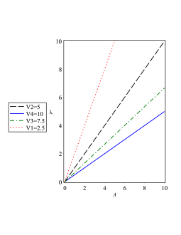
Figure 1: Ratio of expansion coefficient to compression coefficient in non-adiabatic fluid. It is observed that as time passes and the volume increases, the rate of expansion of the universe decreases relative to its compression. The slope of the diagrams is equal to $\frac{C_{p}}{V}$ with $C_{p}$ constant($C_{p}=5$) and $V$ increasing ($V=2.5,5,7.5,10$).

If the fluid is adiabatic, ie we do not have entropy production and the entropy is assumed to be constant and unchanged, then we consider $A=0$. In such a cosmic fluid, the viscosity pressure of the bulk is negative and the pressure decrease continuously in the state of adiabatic expansion, and according to the equation $(59)$ the volume of the fluid increases, in this type of fluid(of course in the adiabatic expansion), the temperature decrease with decreasing pressure and increasing the volume of fluid. The difference between this scenario and the previous scenario is that first, we do not have any entropy production in this type of fluid, but in the previous scenario, which is our acceptable scenario, the entropy increases. The second difference is that the expansion rate in this type of fluid (adiabatic) is more than Non-adiabatic fluid, meaning that the universe expands more rapidly in this scenario and also in previous scenario the temperature was increasing but in this scenario the temperature decrease. However, this scenario can have two specific situations:
Case 1: If the $C_{v}$ is constant and the $C_{p}$ increases then the rate of expansion will be faster with pass the time(Fig. 2. a).
Case 2: If $C_{v}$ decreases and $C_{p}$ is constant: then the rate of expansion increases for a limited time and then begins to compress (Fig. 2. b). This case expresses the dark energy of the phantom well, but is not acceptable in terms of standard cosmological theory. As we can see, the best model for the expansion of the universe is Scenario 1, which is consistent with both cosmological observations and standard cosmological theory. This means that the universe continues to expand, but its rate of expansion increases.

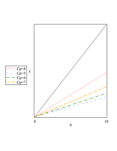
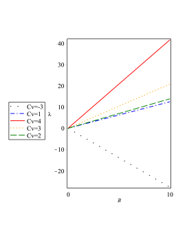
Figure 2: Fig.2.a(Up): The universe expand to infinity. The slope of the diagrams is equal to $\frac{C_{p}^{2}}{VC_{v}}$ that $C_{v}$ is constant($C_{v}=3$) and with increasing volume($V=1,3,6,10$) $C_{p}$ increase.($C_{p}=5,6,7,8)$. Fig.2.b.(Down): The universe expands until a certain time and then stops accelerated expansion and starts to compression.

3.2 Investigation of entropy of dissipative fluids

First, we study the entropy of perfect fluids and then we will investigate the entropy relations in the framework of the two theories of Eckart and IS. For a perfect fluid, in general terms, two expressions of the equation of state, $p=\rho\omega$, with $\omega$ constant and the particle flow number conservation $n^{\alpha}=nu^{\alpha}$, where $u^{\alpha}$ is 4-velocity are considered and we have:

$$\dot{n}+3Hn=\frac{\dot{N}}{N}=0$$ (67)

If we place equations $(67)$ and $(1)$ in the equations of conservation of energy density $(3)$ and the first law of thermodynamics $(4)$, respectively, the following relations are obtained:

$$\dot{\rho}=-3H(p+\rho)$$ (68)

$$TdS=Vd\rho+(p+\rho)dV$$ (69)

that equation $(69)$ is also called the Gibbs relation. Now to calculate the entropy with constant $\omega$ we have

$$TdS=(1+\omega)\rho dV+Vd\rho=U(dLn(\rho)+3(1+\frac{p}{\rho})dLn(a))=0$$ (70)

This equation is obtained from equations $(68)$ and $(69)$. Considering this relation, in this case, if $\omega$ is assumed to be constant, then the entropy is constant, which means that the fluid system is adiabatic, as we saw in scenario 2 in the previous subsection. Now to calculate the constant entropy value, we use the following Eulerian relation:

$$TS=U+\rho V-\mu N$$ (71)

Considering that the temperature and internal energy of a fluid are thermodynamically proportional to each other $(U\propto T)$, hence we can write the following relation:

$$S=(1+\frac{p}{\rho})\frac{U}{T}-\frac{\mu N}{T}=(1+\frac{p}{\rho})\frac{\rho V}{T}-\frac{\mu N}{T}$$ (72)

In perfect cosmic fluids with constant $\omega$, entropy $S$ and the number of fluid particles $N$ are constant, so according to equation (72) the $\frac{\mu}{T}$ ratio must be constant, which $\mu$ is called the chemical potential of the fluid. And based of the chemical potential, three states occur for the cosmic fluid:
1. If $\mu=0$ in this case $p\geq-\rho$ which in this case the cosmic fluid is far from the behavior of the phantom.
2. If $\mu>0$ in this case $p>-\rho$. The entropy has the least constant value and the cosmic fluid in this case does not show the behavior of the phantom.
3. If $\mu<0$ in this case $p<-\rho$. We will have a phantom dark energy or phantom cosmic fluid[25].
In case $\omega$ is the variable $(\omega(a))$, if the chemical potential is $\mu=0$, then the parameter of the variable state, $\omega(a)$, is a constant parameter and is always greater than or equal to $-1$, $\omega(a)\geq-1$, and if $\mu>0$ then $\omega(a)>-1$ and away from the standard state and if $\mu<0$ two states occur, $|\mu|<\frac{S_{0}T}{V_{0}n_{0}}$ which in this case again $\omega(a)>-1$ and if $|\mu|>\frac{S_{0}T}{V_{0}n_{0}}$, we will have the phantom state which in this case will be $\omega(a)<-1$ [25].
Now in the framework of Eckart theory , we investigate the entropy of dissipated cosmic fluids. In this theory, we use equation $(47)$ to calculate the fluid entropy, which in instead of the bulk viscosity pressure $-3H\xi$, therefore we will have:

$$dS=\frac{9H^{2}\xi(t)}{nT}$$ (73)

Now we calculate the thermodynamic variables of density of particles $n$ and temperature $T$ and place them in equation $(73)$, and after we integrate from the obtained equation, finally we obtain the entropy $S$ . In here, we consider two cases:
1. $\xi(t)=\xi_{0}=constant$ and $\xi_{0}>0$ : according to the relations $(3)$ and $(4)$ in the appendix and also the particle density $n=\frac{n_{0}}{a^{3}}$, for $T=T_{0}\rho^{\frac{p_{eff}}{1+p_{eff}}}$ we have:

$$T(t)=T_{0}\rho_{0}^{\frac{p_{eff}}{\rho+p_{eff}}}\times$$

$$[\frac{\xi_{0}e^{\frac{3}{2}\xi_{0}(t-t_{0})}}{H_{0}(1+\frac{p_{eff}}{\rho})(e^{\frac{3}{2}\xi_{0}(t-t_{0})}-1)+\xi_{0}}]^{\frac{2p_{eff}}{\rho+p_{eff}}}$$ (74)

$$n(t)=n_{0}[1+\frac{H_{0}}{\xi_{0}}(1+\frac{p_{eff}}{\rho})(e^{\frac{3}{2}\xi_{0}(t-t_{0})}-1)]^{\frac{-2\rho}{\rho+p_{eff}}}$$ (75)

Now if we place two relations $(74)$ and $(75)$ in relation $(73)$ we have the following relation:

$$\frac{dS}{dt}=\frac{3\xi_{0}\rho_{0}^{\frac{\rho}{\rho+p_{eff}}}}{n_{0}T_{0}}e^{\frac{3\xi_{0}\rho}{\rho+p_{eff}}(t-t_{0})}$$ (76)

If we integrate from equation $(76)$ with assuming $p=-\rho$, the entropy is obtained:

$$S(t)=S_{0}+\frac{(1+\frac{p_{eff}}{\rho})\rho_{0}^{\frac{\rho}{\rho+p_{eff}}}}{n_{0}T_{0}}(e^{\frac{3\xi_{0}\rho}{\rho+p_{eff}}(t-t_{0})}-1)$$ (77)

where $S_{0}$ is a integral constant or the entropy at the present time, now we can see, the increase in entropy is exponential. If in the Eckart theory $\xi$ be variable and according to the hypotheses of the previous section we consider $\xi=\alpha\rho^{s}$ $(\alpha>0)$, similar to the previous case, we get the density of the number of particles $(n)$ and temperature $(T)$ and then we place in $(73)$ and so integrate from the obtained relation to obtain the entropy for the variable $\xi$. Because in this case the coefficient the viscosity of the bulk changes as power-law, choosing a solution to obtain entropy will not be easy, but by giving a specific value for $s$ and $\alpha$, a simpler solution can be expressed. In a particular case, suppose $\alpha=\frac{\sqrt{3}}{3}\gamma$ and $s=\frac{1}{2}$, $\xi=(\frac{\sqrt{3}}{3}\gamma\rho^{\frac{1}{2}})$. Now according to equations $(6)$ and $(7)$ in the appendix to calculate the density of the number of particles $n$, and temperature $T$, and $n=n_{0}a^{-3},T=T_{0}\rho_{0}^{\frac{p_{eff}}{1+p_{eff}}}$ we have:

$$n(t)=n_{0}[1+\frac{3H_{0}}{2}(1+\frac{p_{eff}}{\rho}-\gamma)(t-t_{0})]^{\frac{-2\rho}{\rho+p_{eff}-\gamma}}$$ (78)

,

$$T(t)=T_{0}\rho_{0}^{\frac{p_{eff}}{1+p_{eff}}}[1+\frac{3H_{0}}{2}(1+\frac{p_{eff}}{\rho}-\gamma)(t-t_{0})]^{\frac{-2p_{eff}}{1+p_{eff}}}$$ (79)

If we place the relations $(78,79)$ in $(73)$, we obtain the following differential equation:

$$\frac{dS}{dt}=\frac{\gamma\rho_{0}^{\frac{2\rho+p_{eff}}{\rho+p_{eff}}}}{H_{0}n_{0}T_{0}}\times[1+\frac{3H_{0}}{2}(1+\frac{p_{eff}}{\rho}-\gamma)(t-t_{0})]^{\frac{-(\frac{p_{eff}}{\rho})^{2}+(2-\gamma)(\frac{p_{eff}}{\rho})+1}{(\frac{p_{eff}}{\rho})^{2}+(2-\gamma)(\frac{p_{eff}}{\rho})+(1-\gamma)}}$$ (80)

We integrate from the above relation, therefore we have:

$$S(t)=S_{0}+\frac{(1+\frac{p_{eff}}{\rho})\rho_{0}^{\frac{\rho}{\rho+p_{eff}}}}{n_{0}T_{0}}[(1+\frac{3H_{0}}{2}(1+\frac{p_{eff}}{\rho}-\gamma)(t-t_{0}))^{\frac{\gamma-1}{(\frac{p_{eff}}{\rho})^{2}+(2-\gamma)(\frac{p_{eff}}{\rho})+(1-\gamma)}}-1]$$ (81)

In order for the entropy to increase in this case, the power of equation $(81)$ must be positive.
To calculate the entropy in the Israel-Stuart (IS) theory, we have the following differential equation that it obtain from the placement Ansatz $(41)$ in equation $(46)$, density of the number of fluid particles $(45)$ and the relation $(9)$ in the appendix (temperature relation) in relation $(47)$, then we have:

$$\frac{dS}{dt}=M(t_{\alpha}-t)^{N}$$ (82)

$$M=\frac{(3A^{2})^{\frac{\rho}{\rho+p}}[2+3A(1+\frac{p}{\rho})](t_{\alpha}-t_{0})^{3A}}{n_{0}T_{0}}$$ (83)

$$N=\frac{2p}{\rho+p}-3(1+A)$$ (84)

Now we integrate from equation $(82)$ that we have(with condition $p\neq\rho$):

$$S(t)=S_{0}+(\frac{-M}{N+1})(t_{\alpha}-t)^{1+N}$$ (85)

where $S_{0}$ is an integral constant or entropy at the present time. Here we present two scenarios:
1. If $M>0$ and $N<-1$ then we conclude that $0<\frac{p}{\rho}<\frac{1}{2}$ that we shown in Fig. 3.a. With $\omega>0$ we conclude that the cosmic fluid is expanding.
2. If $M<0$ and $N>-1$. in such a universe, entropy has a constant value and then begins to decrease rapidly which totally violates standard theory and Hubble’s law(Fig.3.b).

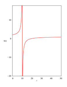
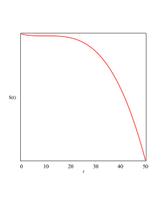
Figure 3: Fig.3.a(Up): Cosmic fluid entropy behavior over time. We see that, the entropy increases infinitely up to a asymptote(here assuming $t=10$ in term of Gpc). Then in the same asymptote, the rate of expansion of the universe equals with its rate of compression and after these asymptote, the average rate of expansion of the universe be lower than the average rate of compression until the average value of entropy production of universe arrives a horizontal asymptote which means that the average rate of expansion of the universe is closer to zero, that we mentioned in the first scenario(for non-adiabatic fluid). with hypothetical conditions[$M=10,N=-2,t_{\alpha}=10,S_{0}=1$]. Fig.3.b.(Down): In this state that it does not correspond to the standard theory at all, the entropy is constant in a limited time and then begins to decrease very rapidly which in fact shows an unreal universe that contradicts Hubble’s law. With hypothetical conditions[$M=-10,N=2,t_{\alpha}=10,S_{0}=1$].

4 The Effects of Energy density for Dark Energy in the IS theory

In this section, we want to investigate the effects of the energy density $\rho$ in the framework of the Israel-Stewart theory. The main parameters that its effects are investigated : temperature $(T)$, bulk viscosity coefficient $(\xi)$ and relaxation time $(\tau)$ (according to equations (29) to (35)). But each of these parameters is obtained in terms of energy density $(\rho)$, so its effects and relationships can be obtained. In this regard, if we rewrite equation $(30)$ as energy density, we have:

$$d\rho=(\frac{\partial\rho}{\partial T})_{n}dT+(\frac{\partial\rho}{\partial n})_{T}dn$$ (86)

We place the density relation of the number of fluid particles $(32)$ and the temperature differential equation $(33)$ in equation $(86)$, we have:

$$d\rho=-3H[(p+\rho+\Pi)+n(\frac{\partial\rho}{\partial T})_{n}(\frac{\partial T}{\partial n})_{\rho}-n(\frac{\partial\rho}{\partial n})_{T}]$$ (87)

that we simplify this equation, we get the equation of conservation of energy density in equation $(31)$:

$$d\rho=-3H(p+\rho+\Pi)$$

Due to the bulk viscosity pressure in the Israel-Stewart (IS) theory, we have two states:
Mode 1: $\Pi=-2\dot{H}-3(1+\frac{p}{\rho})H^{2}$ (according to the equation $(36)$), we place this value $\Pi$ in the energy density conservation equation $d\rho$ we have:

$$d\rho=-3H(p+\rho-2\dot{H}-3H^{2}(1+\frac{p}{\rho}))$$ (88)

Now we integrate from the above relation twice, then we have:

$$\rho(a)=\frac{9}{20}(1+\frac{p}{\rho})H^{5}+(-\frac{1}{2}(p+\rho)+1)H^{3}$$ (89)

In following, we summarize the results according to table $(1)$. Also we plotted the obtained results in figure $(4)$. According to figure $(4A)$ that shows the energy density in term of scale factor in standard approach. The condition of the universe expansion and increase of the scale factor is the ascending increase of the value of energy density. In this approach, the pressure value is symmetrical with energy density value and with the energy density value increase, the value of pressure becomes more negative. In figure $(4B)$ that shows the energy density in term of scale factor in dynamical and non-phantom approach. In this figure pressure value is greater than the energy density value, with the universe expansion and the scale factor increase, the energy density value increases similar in the standard approach. But in this case as much as the energy density value be lower, the universe expands faster. Finally, figure $(4C)$ shows the energy density in the phantom approach, with the universe expansion and the scale factor increase, the energy density value increases but in this case as much as the energy density value be more, the universe expand faster and also if the energy density value exceeds a certain value, the universe stops accelerated expansion and begins to slow expansion and when energy density value becomes infinite, the universe will reach a big rip singularity in the future.

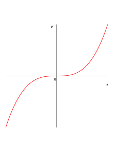
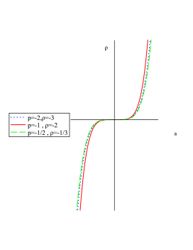
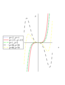
Figure 4: The effects of energy density in term of scale factor on the universe expansion in Israel-Stewart theory(IS) Fig.4.A(up): standard approach with condition $p=-\rho$, Fig.4.B(middle): dynamical and non-phantom approach with condition $p>-\rho$, Fig.4.C(down): phantom approach with condition $p<-\rho$.

Mode $2$: $\Pi(t)=A(2+3A(1+\frac{p}{\rho}))(t_{\alpha}-t)^{2}$ (according to the equation $(46)$), we place this relation in the energy density conservation equation $d\rho$ so we have:

$$d\rho=-3H[p+\rho+A(2+3A(1+\frac{p}{\rho}))(t_{\alpha}-t)^{2}]$$ (90)

And, as we know, $t_{\alpha}$ is a time that leads to a singularity in the future, and $A$ is a constant that describes the expansion of the universe(its value was obtained in equation $(43)$). Now if we integrate from the above relation we have:

$$\rho(t)=-3H[pt+\rho t-\frac{1}{3}A(2+3A(1+\frac{p}{\rho}))(t_{\alpha}-t)^{3}]$$ (91)

Table 1: The results of the energy density effects in terms of scale factor on the universe expansion in the framework of IS theory (Mode 1).

Condition	Approach	Description
$P=-\rho$	Standard	In this case, the parameter of the cosmic fluid state equation ($\omega$) is considered constant as dark energy with bulk viscosity and its value is $\omega=-1$ and according to equation (1) it becomes $p=-\rho$ and also has no dynamics. In this type of approach the pressure value of cosmic fluid is negative and energy density increases and finally, the universe continues the expansion rapidly.
$P>-\rho$	Dynamical and non-phantom	In this approach, first the parameter $\omega$ is not constant and increase with the expansion of the universe, that is, as the universe expands, the pressure of the cosmic fluid with bulk viscosity tends from negative to positive value. This means that the energy density value decreases. Second, this approach conforms to the thermodynamics laws and the standard cosmological model and also shows that as the universe expands, the entropy and temperature increase and the chemical potential becomes negative [24],[25].
$P<-\rho$	Phantom	The energy density of a cosmic fluid increases as power-law($\rho=\rho_{0}a^{r}$), that r is a constant and positive, and $\rho_{0}$ is the initial value of the energy density of the fluid. In this approach, with the growth of the scale factor and the expansion of the universe, the energy density increases and leads to decrease in temperature and no entropy is produced. The rate of expansion in this approach is much higher and leads to a big rip singularity. This approach also violates the dominant energy conditions (DEC) and faces with many challenges and are classically and quantum unstable.[14]

We obtain the following results according to table $(2)$, we also plotted the obtained results and relations in figure $(5)$.
In this mode, and figure $(5A)$ the results are similar to the standard approach in table$(1)$, but with the difference that in previous mode the energy density was in terms of scale factor but here in terms of cosmic time and an expansion coefficient $A$ that obtained in the second section. In figure $(5B)$ with over time and the universe expansion, the energy density value decreases so the pressure value increases and tends to be positive. Finally, in figure $(5C)$ with over time, the energy density value increases and as a result the universe is expanded faster but when it crosses the phantom divide line (here the phantom divide line has been showed by a black dotted line on the $\rho$ axis) and the energy density becomes infinity, the universe begins to slow expansion until it finally reaches a big rip singularity at the time $t_{\alpha}$. In this section we could to study the effects of energy density in terms of scale factor and in terms of cosmic time on the expansion of the universe under the Israel-Stewart (IS) theory.
Here, Let us compared results of our research with earlier studies of Dark Energy from viscous or inhomogeneous fluids according references [48,49,50]. In this regard, Brevik et al considered the role of a viscous (or inhomogeneous (imperfect) equation of state) fluid in a Little Rip cosmology. Despite the earlier observations that viscosity basically supports the Big Rip singularity, they have demonstrated that it is also able to give rise to a non-singular, Little Rip cosmology, which is considered to be a viable alternative to $\Lambda$CDM cosmology. In particular, constant bulk viscosity and a viscosity inversely proportional to the Hubble rate have been considered. They have shown that in those cases a Little Rip cosmology may naturally emerge. It is remarkable that for a standard fluid, $p=\omega\rho$, the only influence of viscous effects can naturally drive the universe to a Little Rip type evolution[48]. Also, Brevik and Timoshkin studied a general equation of state for the dark fluid in the presence of a bulk viscosity. They have explored the holographic principle for cosmological models with various values for the thermodynamic parameter $\omega(\rho,t)$ and for different forms of the bulk viscosity $\zeta(H,t)$. For each model the infrared radius, in the form of a particle horizon, has been calculated in order to obtain the energy conservation law. Thus, they have shown the equivalence between viscous models and the holographic model[49]. Finally, Nojiri et al in [50] considered the effect of modification of general equation of state of dark energy ideal fluid by the insertion of inhomogeneous, Hubble parameter dependent term in the late-time universe. Several explicit examples of such term which motivated by time-dependent bulk viscosity or deviations from general relativity studied. The corresponding late-time FRW cosmology (mainly, in its phantom epoch) described. Also, they found that the inhomogeneous term in equation of state helps to realize such a transition in a more natural way. It is interesting that in the case when universe is filled with two interacting fluids (for instance, dark energy and dark matter) the Hubble parameter dependent term may effectively absorb the coupling between the fluids [50].
In comparing of above results with our findings in section 4, we can point out in summary : 1- In standard approach, with over time, the universe has an accelerated expansion (of course, before time $t_{\alpha}$). After time $t_{\alpha}$, we assume that over time pressure tends to $p\rightarrow-2\rho$ and the universe expand slowly. In this approach the energy density value increases rapidly but its value is symmetrical with the value of negative pressure. 2- In dynamical and non-phantom approach, with over time, the pressure value is negative and will change with the energy density value, and expansion will increase, and as a result, the energy density will decrease. Therefore, the condition for the expansion of the universe with over time is the decrease in the dark energy density variable value. As much as the energy density value is lower, the universe expand faster. 3- In phantom approach, with over time, the energy density becomes bigger and tends to be infinity. As a result, the universe expands more rapidly, but after crossing the phantom divide line, the value of energy density becomes infinity(the maximum value of energy density), the universe’s expansion rate gradually decreases and finally reaches a big rip singularity after time $t_{\alpha}$ [51].

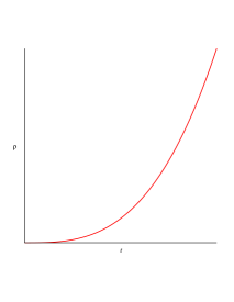
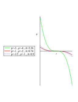
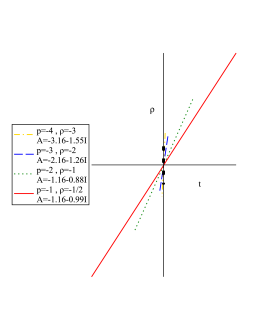
Figure 5: The effects of energy density in term of cosmic time on the universe expansion in Israel-Stewart theory(IS). Fig.5.A(up): standard approach with condition $p=-\rho$ and $A=\frac{1}{3}\mp\frac{1}{6\sqrt{\rho}}$, Fig.5.B(middle): dynamical and non-phantom approach with condition $p>-\rho$ and $A>\frac{1}{3}\mp\frac{1}{6\sqrt{\rho}}$, Fig.5.C(down): phantom approach with condition $p<-\rho$ and $A<\frac{1}{3}\mp\frac{1}{6\sqrt{\rho}}$. In this mode we considered the value of $t_{\alpha}=10$ and value of the Hubble constant $H\simeq 71\times 10^{9}$.

Table 2: The results of the energy density effects in terms of cosmic time on the universe expansion in the framework of IS theory (Mode 2).

Condition	Approach	Description
$P=-\rho\newline A=\frac{1}{3}\mp\frac{1}{6\sqrt{\rho}}$	Standard	In this case, it is the same as in Table (1), except that the energy density is measured in terms of scale factor, but here it is defined by cosmic time and also a constant A. With Over time, the universe has an accelerated expansion (of course, before time $t_{\alpha}$). After time $t_{\alpha}$, we assume that over time pressure tends to $p\longrightarrow-2\rho$ and the universe expand slowly. In this approach the energy density value increases rapidly but its value is symmetrical with the value of negative pressure.
$P>-\rho\newline A>\frac{1}{3}\mp\frac{1}{6\sqrt{\rho}}$	Dynamical and non-phantom	In this case, with over time, the pressure value is negative and will change with the energy density value[20], and expansion will increase, and as a result, the energy density will decrease (according to condition A). Therefore, the condition for the expansion of the universe with over time is the decrease in the dark energy density variable value. As much as the energy density value is lower, the universe expand faster.
$P<-\rho\newline A<\frac{1}{3}\mp\frac{1}{6\sqrt{\rho}}$	Phantom	In this case, with over time, the energy density becomes bigger and tends to be infinity. As a result, the universe expands more rapidly, but after crossing the phantom divide line [21], the value of energy density becomes infinity(the maximum value of energy density), the universe’s expansion rate gradually decreases and finally reaches a big rip singularity after time $t_{\alpha}$.

5 Summary

In accordance with the unknown nature of dark energy, some dark energy models has been studied as a cosmic fluid in the framework of thermodynamic laws. In this regard, viscosity is a feature of the universe fluid content as discussed in the present research. Therefore, in the first part of this article, we expressed the thermodynamics of cosmic fluids in general with a constant and variable equation of state under the two theories of Eckart and Israel-Stewart. Then, we examined the dissipative effects of cosmic fluids and finally examine the effects of energy density for dark energy in the Israel-Stewart(IS) theory. The results are organized as follows:
We first investigated the thermodynamics of cosmic fluids in the dark energy bulk viscosity model and the general relationships. Then, we expressed the thermodynamic relationships of Eckart’s theory. In IS theory, a differential equation is defined in terms of temperature $(T)$, bulk viscosity coefficient $(\xi)$ and relaxation time $(\tau)$, and each of these parameters is obtained in terms of energy density. First time, we obtained an equation for the bulk viscosity pressure by placing the value of $s=1$ in equation $(37)$ and the Ansats solution.
In the third section, we investigated the dissipative effects of cosmic fluids and we concluded the best theory for studying the effects of dissipation is IS theory, because it develops dissipation processes with slower rate. In this section, We presented two scenarios. In the first scenario, we considered the cosmic fluid to be non-adiabatic. We concluded that this type of fluid conforms to the standard model of cosmology and cosmic observations, which during it, entropy and temperature increase and causes the universe to expand. But in the second scenario, we considered the cosmic fluid to be adiabatic and concluded that no entropy is produced in this scenario and temperature decreases. Also, we defined two states in this scenario, one is the accelerated expansion state and the other is a phantom state that leads to a singularity at the late of the universe. In the continuation of the third section, we investigated the effects of cosmic fluid entropy in general and then in the framework of Eckart and IS theories. We concluded that IS theory better represents the production of entropy in dissipated cosmic fluids. Also, in this part we defined two different scenarios for entropy. The first scenario represents more correct behavior from cosmic fluid entropy with over time but the second scenario is completely opposite to the first scenario.
In the fourth section, first time we expressed the effects of energy density on the expansion of the universe in the framework of IS theory. According to the definition of bulk viscosity pressure in IS theory, we suggested two modes, one is energy density in terms of scale factor and the other is energy density in terms of cosmic time and an expansion descriptor coefficient $(A)$. The obtained results in this section are comprehensively presented in two tables $(1)$ and $(2)$. We also plotted the energy density behavior in three standard, dynamical and phantom approaches and obtained its results.

Acknowledgements We would like to thank all those who helped us gather the information needed for this research.
Funding The authors did not receive support from any organization for the submitted work.
Data availability The data that support the findings of this study are available on request from the corre- sponding author.
Conflict of interest The authors declare that they have no known competing financial interests or personal relationships that could have appeared to influence the work reported in this paper. This research did not receive any specific grant from funding agencies in the public, commercial, or not-for-profit sectors.
Ethics approval We have followed all the rules stated in the Ethical Responsibilities of Authors section of the journal.
Consent for publication We consent to the publication of this manuscript with the rules of the journal.

6 Appendix

In this section, we consider some equations that were involved in obtaining the equations in the previous sections. To calculate entropy we need to calculate the particles number density of the fluid and the temperature of the fluid. According to equation $(33)$ and its solution $(T=T_{0}\rho^{\frac{p}{p+\rho}})$ we can write:

$$\dot{T}=(\frac{p}{p+\rho})T\frac{\dot{\rho}}{\rho}+\rho^{\frac{p}{p+\rho}}\frac{df}{dx}\dot{x}$$ (1)

where $df$ is a function in term of $x=T_{0}\rho^{\frac{p}{p+\rho}}$ and also according to equations $(3)$ and $(32)$ we can write for $\dot{x}$:

$$\dot{x}=\frac{\rho^{\frac{p}{p+\rho}}}{n}[(\frac{\rho}{p+\rho})\frac{\dot{\rho}}{\rho}-\frac{\dot{n}}{n}]=0$$ (2)

then appendix equation (1) becomes equation $\frac{dT}{T}=-3\frac{p+\rho}{\rho}\frac{da}{a}=\frac{p}{p+\rho}\frac{d\rho}{\rho}$ in the bulk viscosity model of a fluid with coefficient $\xi$ that $\xi$ is constant to calculate Hubble parameter and scale factor, we have(which equations $(74)$ and $(75)$ are concluded from them) [18]:

$$H(t)=\frac{H_{0}\xi_{0}e^{\frac{3\xi_{0}(t-t_{0})}{2}}}{H_{0}(\frac{p+\rho}{\rho})(e^{\frac{3\xi_{0}(t-t_{0})}{2}}-1)+\xi_{0}}$$ (3)

$$a(t)=(1+\frac{H_{0}(p+\rho)}{\xi_{0}\rho}(e^{\frac{3\xi_{0}(t-t_{0})}{2}}-1))^{\frac{2\rho}{3(p+\rho)}}$$ (4)

which by integrating the Hubble parameter relation, the scale factor is obtained with condition $a(t_{0})=1$.
Finally, the energy density of the fluid can be obtained in term of scale factor:

$$\rho(a)=\rho_{0}(\frac{\xi_{0}\rho}{H_{0}(p+\rho)}+(\frac{H_{0}(p+\rho)-\xi_{0}\rho}{H_{0}(p+\rho)})a^{\frac{-2\rho}{3(p+\rho)}})^{2}$$ (5)

Now, if $\xi$ is assumed to be variable as power-law,$\xi=\alpha\rho^{s}$,we will have [18]:

$$H(t)=H_{0}(1+\frac{3H_{0}}{2}(\frac{p+\rho}{\rho}-\alpha)(t-t_{0}))^{-1}$$ (6)

$$a(t)=(1+\frac{3H_{0}}{2}(\frac{p+\rho}{\rho}-\alpha(t-t_{0})))^{\frac{2}{3(\frac{p+\rho}{\rho}-\alpha)}}$$ (7)

$$\rho(a)=\rho_{0}a^{-3(\frac{p+\rho}{\rho}-\alpha)}$$ (8)

To calculate the fluid temperature in the bulk viscosity model in Israel-Stewart(IS) theory in term of scale factor according to the relations $(41)$, $(44)$ and $T=T_{0}\rho^{\frac{p}{p+\rho}}$ we will have:[16]

$$T(t)=\tilde{T}(3A^{2})^{\frac{p}{p+\rho}}(t_{\alpha}-t)^{\frac{-2p}{p+\rho}}=\tilde{T}(3A^{2}(t_{\alpha}-t)^{-2})^{\frac{p}{p+\rho}}a^{\frac{2p}{A(p+\rho)}}$$ (9)

References

- [1] A. G. Riess et al. , Observational evidence from supernovae for an accelerating universe and a cosmological constant, Astron. J. 116 (1998) 1009.
- [2] S. Perlmutter et al. , Measurements of Omega and Lambda from 42 high redshift supernovae,Astrophys. J. 517 (1999) 565.
- [3] D. N. Spergel et al. , Three-Year Wilkinson Microwave Anisotropy Probe (WMAP) Observations:Implications for cosmology, Astrophys. J. Suppl. 170 (2007) 377.
- [4] M. Tegmark et al. , Cosmological parameters from SDSS and WMAP, Phys. Rev. D 69 (2004) 103501.
- [5] S. Capozziello, V. F. Cardone, E. Piedipalumbo and C. Rubano, Dark energy exponential potential models as curvature quintessence, Class. Quantum Grav. 23 (2006) 1205.
- [6] Yu. Zhang and Y. X. Gui, Quasinormal modes of gravitational perturbation around a Schwarzschild black hole surrounded by quintessence, Class. Quantum Grav. 23 (2006) 6141.
- [7] R. R. Caldwell, M. Kamionkowski and N. N. Weinberg, Phantom energy: dark energy with causes a cosmic doomsday, Phys. Rev. Lett. 91 (2003) 071301.
- [8] R. J. Scherrer, Purely kinetic k Essence as unified dark matter, Phy. Rev. Lett. 93 (2004) 011301.
- [9] M. R. Setare, Interacting holographic generalized Chaplygin gas model, Phys. Lett. B, 654 (2007) 1.
- [10] S. Nojiri and S. D. Odintsov, Introduction to modified gravity and gravitational alternative fordark energy, Int. J. Geom. Methods Mod. Phys. 4 (2007) 115.
- [11] T. P. Sotiriou and S. Liberati, Metric-affine f(R) theories of gravity, Ann. Phys. 322 (2007) 935.
- [12] H. Wei, R. -G. Cai and D. -F. Zeng, Hessence: a new view of quintom dark energy, Class. Quantum Grav. 22 (2005) 3189.
- [13] M. Li, A model of holographic dark energy, Phys. Lett. B 603 (2004) 1.
- [14] R. Crittenden, Lecture Notes in Physics, 720 187 (2007).
- [15] K. Bamba, S. Capozziello, S. Nojiri and S. D. Odintsov, Dark energy cosmology: the equivalent description via different theoretical models and cosmography tests, Astrophys. Space Sci. 342 (2012) 155-228.
- [16] I. Brevik, et al, Viscous cosmology for early- and late-time universe, Int. J. Mod. Phys. D 26 (2017) no.14 1730024.
- [17] Y. B. Zeldovich and I. D. Novikov, Relativistic Astrophysics. Vol. 2. The Structure And Evolution Of The Universe,Chicago, USA: Chicago Univ. (1983) 718p.
- [18] D. Tamayo, Thermodynamics of viscous dark energy for the late future time universe, Rev. Mex. Fis. 68 (2022) 2.
- [19] C. Eckart, The Thermodynamics of Irreversible Processes, Phys. Rev. 58 (1940) 267.
- [20] W. Israel and J. M. Stewart, Thermodynamics of nonstationary and transient effects in a relativistic gas, Phys. Lett. A 58 (1976) 213.
- [21] J. S. Gagnon and J. Lesgourgues, Dark goo: bulk viscosity as an alternative to dark energy, JCosmol. Astropart. Phys. 09 (2011) 026.
- [22] G. Zhao, et al, Nat. Astron. 1 (2017) no. 9, 627-632.
- [23] Y. Wang, L. Pogosian, G. Zhao and A. Zucca, Astrophys. J. 869 (2018) L8
- [24] R. C. Duarte, E. M. Barboza, E. M. C. Abreu andJ. A. Neto, Eur. Phys. J. C 79 (2019) no. 4, 356.
- [25] H. H. B. Silva, R. Silva, R. S. Gonalves, Z. H. Zhu andJ. S. Alcaniz, Phys. Rev. D 88 (2013) 127302.
- [26] J. D. Barrow, Nucl. Phys. B 310 (1988) 743-763.
- [27] N. Cruz, S. Lepe, Phys. Lett. B 767 (2017) 103.
- [28] A. B. Balakin, D. Pavon, D. J. Schwarz and W. Zimdahl,New J. Phys. 5 (2003) 85.
- [29] I. H. Brevik and O. Gorbunova, Gen. Rel. Grav. 37 (2005) 2039.[gr-qc/0504001]
- [30] I. Brevik, Front. in Phys. 1 (2013) 27.
- [31] A. Avelino and U. Nucamendi, JCAP 1008 (2010) 009.
- [32] N. Bilic, Fortsch. Phys. 56 (2008) 363-372.
- [33] E. N. Saridakis, P. F. Gonzalez-Diaz and C. L. Siguenza,Class. Quant. Grav. 26 (2009) 165003.
- [34] V. F. Cardone, N. Radicella and A. Troisi, Entropy 19(8) (2017) 392.
- [35] S. Lepe, G. Otalora and J. Saavedra, Phys. Rev. D 96 (2017) no. 2, 023536.
- [36] W. Yang, S. Pan, E. Di Valentino, A. Paliathanasis and J. Lu, Phys. Rev. D 100 (2019) no. 10, 103518.
- [37] R. Maartens, Class. Quantum Grav. 12 (1995) 1455-1465.
- [38] M. Cataldo, N. Cruz and S. Lepe, Phys. Lett. B 619 (2005) 5-10.
- [39] J. D. Barrow, Phys. Lett. B 180 (1986) 335-339.
- [40] M. Cruz, N. Cruz and S. Lepe, Phys. Rev. D 96 (2017) no. 12, 124020.
- [41] S. Nojiri,S. D. Odintsov,S. Tsujikawa, Phys. Rev. D 71 (2005) 063004.
- [42] M. Cruze,N. Cruze and S. Lepe, Phys. Lett. B 769 (2017) 159-165.
- [43] P. Bhandari, S. Haldar, S. Chakraborty, Eur. Phys. J. A 54 (2018) 78
- [44] W. Zimdahl and D. Pav´on, Phys. Rev. 61, 108301 (2000).
- [45] S. Weinberg, ”Entropy generation and the survival of protogalaxies in an expanding universe,” Astrophys. J., 168 (1971) 175.
- [46] H. B. Callen, Thermodynamics and an Introduction to Thermostatistics, 2nd ed. (Wiley, N. Y. 1985).
- [47] R. Kubo, Thermodynamics: An Advanced course with Problems and Solutions (North-Holland Publishing Company, Amsterdam, 1968).
- [48] I. Brevik, E. Elizalde, S. Nojiri, and S. D. Odintsov, Viscous little rip cosmology, Phys. Rev. D 84 (2011) 103508.
- [49] S. Nojiri and S. D. Odintsov, Inhomogeneous equation of state of the universe: Phantom era, future singularity, and crossing the phantom barrier, Phys. Rev. D 72 (2005) 023003.
- [50] I. Brevik and A. V. Timoshkin, Holographic representation of the unified early and late universe via a viscous dark fluid, Int. J. Geom. Meth. Mod. Phys. 19 (2022) 2250113.
- [51] S. Capozziello, et al, Observational constraints on dark energy with generalized equations of state, Phys. Rev. D 73 (2006) 043512.