Perturbative Analysis of Quasi-periodic Patterning of Transmon Quantum Computers: Enhancement of Many-Body Localization

Abstract

Recently it has been shown that transmon qubit architectures experience a transition between a many-body localized and a quantum chaotic phase. While it is crucial for quantum computation that the system remains in the localized regime, the most common way to achieve this has relied on disorder in Josephson junction parameters. Here we propose a quasi-periodic patterning of parameters as a substitute for random disorder. We demonstrate, using the Walsh-Hadamard diagnostic, that quasiperiodicity is more effective at achieving localization. In order to study the localizing properties of our new Hamiltonian for large, experimentally relevant system sizes, we develop a many-body perturbation theory whose computational cost scales only like that of the corresponding non-interacting system.

Despite immense advances in quantum computing using the superconducting qubit platform [1, 2, 3], two-qubit gate fidelity remains a thorn in the side of further progress with these devices. One prominent source of these errors is quantum cross talk in the form of qubit $ZZ$ couplings [4], with $Z$ denoting the Pauli $z$ operator. This cross talk is the result of always-on coupling of qubits, even in idle mode. There are two primary strategies for dealing with these residual couplings, tunable coupling [5] and static coupling between opposite anharmonicity qubits [6, 7]. Each of these coming with disadvantages: additional hardware overlay of couplers for the former and lower coherence time of capacitively shunted flux qubits for the latter. In real devices the existence of natural random disorder is unavoidable and most prominently present in the critical current of Josephson junctions. Even thought in modern devices tuning of Josephson junctions is possible, even post fabrication, with laser annealing techniques [8], some degree of residual disorder remains.

The many body system formed by a network of $N$ Josephson qubits, with random disorder and fixed coupling, is a prime candidate for quantum chaos. Recently it has been established that there is in fact a phase transition between quantum chaotic and many body localization (MBL) for transmon arrays [9] of this type. The phenomenology of this transition can be summarised by considering the diagonalized Hamiltonian of such a multiqubit system

$$H=\sum_{a\in\mathbb{B}^{N}}E_{a}|a\rangle\langle a|=\sum_{b\in\mathbb{B}^{N}}w_{b}Z_{1}^{b_{1}}\dots Z_{N}^{b_{N}},$$ (1)

where $\mathbb{B}^{N}$ is the set of all bit-strings of length $N$, $w_{b}$ is a real coefficient corresponding to bit-string $b$, $b_{i}$ is the $i$-th digit of bit-string $b$, and $Z_{i}$ is the Pauli $z$ operator acting on the subspace of qubit $i$. The coefficients $w_{b}$ with a bit-string $b$ consisting of only two 1s in adjacent sites correspond, by definition, to the $ZZ$-couplings. Longer range $ZZ$ couplings or higher weight terms have generally been neglected, a treatment which is consistent in the MBL phase where we have an exponential hierarchy of these terms with respect to correlation range [10, 11]. This is in stark contrast with the chaotic regime however, where all of these terms are of the same order of magnitude.

These systems can only be deep in the MBL phase due to the happenstance of disorder in the energies $E_{J}$ of the Josephson qubits. In this paper we explore the stabilization of the MBL phase with a quasi-periodic potential replacing the randomly chosen disorder potential and determine that there is in fact a robust localized regime. We develop a new bosonic variant of Møller-Plesset perturbation theory [12] to treat this localized regime, obtaining the energy levels of the qubit sector of the system. This perturbation theory directly determines the coefficients $w_{b}$ of Eq. (1) via the Walsh-Hadamard transform

$$w_{b}=\frac{1}{2^{N}}\sum_{a\in\mathbb{B}^{N}}(-1)^{b\cdot\bar{a}}E_{a}$$ (2)

with $\bar{a}$ denoting a bit-string resulting from flipping each digit of bit-string $a$ . Finally, we demonstrate the accuracy of this perturbative calculation of the Walsh-Hadamard coefficients and apply it for larger system sizes, beyond what can be explored with exact diagonalization techniques.

Methodology: Here we focus on capacitively coupled transmon arrays. The minimal model Hamiltonian for such an array [14, 15] is

$$H=4E_{\text{C}}\sum_{i=1}^{N}n_{i}^{2}-\sum_{i=1}^{N}E_{\text{J}_{i}}\cos(\phi_{i})+\lambda\sum_{\langle i,j\rangle}n_{i}n_{j},$$ (3)

where $n_{i}$ is the Cooper-pair number of site $i$ and $\phi_{i}$ is the conjugate variable, corresponding to the superconducting phase. $E_{\text{C}}$ is the capacitive energy of each transmon, which is considered to be equal for all sites of the array. $E_{\text{J}_{i}}$ is the Josephson energy of site $i$ and finally $\lambda$ is the constant coupling strength between sites. We also assumed only nearest neighbor coupling.

Recasting this Hamiltonian in second quantization form, expanding the cosine term only up to second order and employing a rotating wave approximation we obtain

$$H_{0}=\sum_{i=1}^{N}\omega_{i}a_{i}^{\dagger}a_{i}+J\sum_{\langle i,j\rangle}a_{i}^{\dagger}a_{j}.$$ (4)

This Hamiltonian is the usual tight binding model that is used in Anderson-localization studies [16, 17]. Note that the ladder operators are bosonic — we are not restricted to the single-excitation manifold of the Fock space. Strictly speaking, the new coupling strength $J$ would be bond-dependent and proportional to $\lambda\sqrt{\omega_{i}\omega_{j}}/E_{\text{C}}$ with $\omega_{i}=\sqrt{8E_{\text{J}_{i}}E_{\text{C}}}$. Here we have omitted this bond dependence in order to simplify the calculations. We find that this does not substantially alter our results.

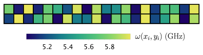
Figure 1: Metallic-Aubry-André disorder potential: Transmon frequency disorder potential $\omega(x_{i},y_{i})$ (Eq. (5)) for a quasi-1D lattice of dimensions $2\times 20$. We use mean frequency $\langle\omega\rangle=5.5\text{ GHz}$ and disorder strength $\Delta=1\text{ GHz}$. The on-site frequencies are color-coded according to the given color bar and the values are given in GHz. The bottom row of the lattice corresponds to $y=1$ and the top to $y=2$. The leftmost sites of the lattice have $x=1$ and the rightmost $x=20$.

In order to design a frequency pattern for our transmon arrays, which should serve as a localizing disorder potential, the essential feature is to make it non repeating in order to avoid resonances. A secondary objective is to avoid having near-resonant sites in physical proximity for some specific lattice geometry. Our reasons for this will become clear later. Here we focus on a quasi-1D square lattice with dimensions $2\times L$ as the one depicted in Fig. 1. Such a lattice geometry is already in use for actual quantum computing devices [18] and may also become even more relevant for future designs. Using integer-valued real space coordinates $(x_{i},y_{i})$ for site $i$, where $y$ is the short axis and $x$ the long axis of length $L>2$, we introduce the “disorder” potential

$$\omega(x_{i},y_{i})=\langle\omega\rangle+\frac{\Delta}{2}\sin\left[\pi\left(y_{i}+\sqrt{y_{i}^{2}+4}\right)x_{i}\right].$$ (5)

Here $\langle\omega\rangle$ is the central value around which the transmon frequencies fluctuate with a disorder strength that is determined by the sine function amplitude $\Delta$.

The inspiration behind using this potential is the Aubry-André model commonly used in the study of 1D quasi-crystals where it exhibits a well studied transition between Anderson localized and delocalized phases [19, 20, 21, 22, 23]. As a matter of fact, treating the $y$ coordinate as a fixed parameter we recover the exact form of the Aubry-André model. In other words, along the $x$ direction, the disorder potential is Aubry-André while changing the $y$ coordinate simply changes the period of the sine function. In order for the potential to be non-periodic, the periodicity of the sine function must be chosen so that it is incommensurate with the integer periodicity of the lattice. This is done here by making the periodicity irrational, and since we need the periodicity to be varying with $y$ we need a family of irrational numbers, hence our choice of the metallic ratios [24].

We need to include many-body contributions in our model, which means anharmonicity effects. Thus, we must further expand the cosine of Eq. (3) at least to fourth order, at which point we end up (after further rotating-wave approximations) with the Bose-Hubbard Hamiltonian

$$H_{\text{BH}}=H_{0}-\frac{E_{\text{C}}}{2}\sum_{i=1}^{N}a_{i}^{\dagger}a_{i}(a_{i}^{\dagger}a_{i}+1).$$ (6)

Using this Hamiltonian as an effective description of our system, we will obtain the Walsh-Hadamard coefficients perturbatively in the anharmonicity. Even though the capacitive energy $E_{\text{C}}$ is not the smallest energy scale in our system the use of perturbation theory is justified as long as we are in the transmon regime since $E_{\text{C}}/\omega_{i}\sim\sqrt{E_{\text{C}}/E_{\text{J}_{i}}}\ll 1$.

For the Walsh-Hadamard coefficients of Eq. (2) we only need to obtain the perturbed energy levels that correspond to qubit states $|b\rangle$. For example, the first order perturbation theory correction is

$$E_{b}^{(1)}=-\frac{E_{\text{C}}}{2}\sum_{i=1}^{N}\langle b|a_{i}^{\dagger}a_{i}|b\rangle-\frac{E_{\text{C}}}{2}\sum_{i=1}^{N}\langle b|a_{i}^{\dagger}a_{i}a_{i}^{\dagger}a_{i}|b\rangle,$$ (7)

with $b$ standing for a bit-string of length equal to the number of lattice sites $N$. Therefore, before we proceed with any calculation it is crucial to address the issue of how to identify the qubit states $|b\rangle$ and distinguish them from non-computational states.

Labeling a state with a bit-string might misleadingly imply that it is an eigenstate of the local particle number operator $a_{i}^{\dagger}a_{i}$ of the bare basis in Eq. (4). But as seen in Eq. (7), $|b\rangle$ is rather an eigenstate of the non-interacting Hamiltonian $H_{0}$ (Eq. (4)). Therefore $|b\rangle$ is an eigenstate of the local particle number operator in the dressed basis

$$|b\rangle=\prod_{\mu=1}^{N}(c_{\mu}^{\dagger})^{b_{\mu}}|0\rangle,$$ (8)

where $b_{\mu}$ is the $\mu$-th digit of bit-string $b$ and $c_{\mu}^{\dagger}$ is the creation operator of single-excitation eigenstate $\mu$ of $H_{0}$

$$H_{0}=\sum_{\mu=1}^{N}E_{\mu}c_{\mu}^{\dagger}c_{\mu}.$$ (9)

For sufficiently weak transmon coupling $J$ our system should be localised and the dressed basis should be nearly identical to the bare basis $c_{\mu}^{\dagger}=a_{\mu}^{\dagger}+O(J/\Delta)$. By definition

$$c_{\mu}^{\dagger}|0\rangle\stackrel{{\scriptstyle!}}{{=}}\left(\sum_{i=1}^{N}\psi_{\mu}(x_{i},y_{i})a_{i}^{\dagger}\right)|0\rangle,$$ (10)

meaning that $c_{\mu}^{\dagger}$ generates a single-excitation eigenstate $|\psi_{\mu}\rangle$ of $H_{0}$, which is exponentially localised around lattice site $\mu$ with coordinates $(x_{\mu},y_{\mu})$. To avoid any possible confusion we will reserve Latin indices for the bare basis and Greek indices for the dressed basis.

Starting from Eq. (10) it is straightforward to find the inverse transformation, as demonstrated in the supplemental material Eqs. (S3) and (S4), and express every term of the perturbative expansion in the dressed basis. Such a substitution yields vacuum expectation values of ladder operator products which can be calculated by means of Wick contractions. These ladder operator products consist of external operators and internal operators. We define the external operators as the $N$ annihilation operators coming from $\langle b|$ and the $N$ creation operators from $|b\rangle$, while the internal operators are the ones that originate from the perturbation term. However, since the external operators appear with an undetermined exponent that can be either 0 or 1, it is beneficial to use a generalised type of Wick contraction rules rather than exhausting all possible combinations which grow exponentially with system size. These rules are

$$\wick{\c{1}{c}_{\mu}^{b_{\mu}}(\c{1}{c}_{\nu}^{\dagger})^{b_{\nu}}}=b_{\mu}b_{\nu}\delta_{\mu\nu}$$ (11)

and all other possible contractions are vanishing. With these rules at hand the relevant amplitudes can be calculated using the method described in [25] inductively.

In order to carry out this calculation we therefore only need to obtain the single-particle sector eigenenergies $E_{\mu}$ and eigenstates $|\psi_{\mu}\rangle$. Since we are only interested in the localised regime of the system, we could obtain those perturbatively as well in the coupling $J$. However this adds one additional layer of complexity for our final expressions without leading into any particular new insights. Therefore we choose to obtain the single-particle sector spectrum numerically and use these results as input to our derived analytic expressions from second order perturbation theory in the anharmonicity $E_{\text{C}}$.

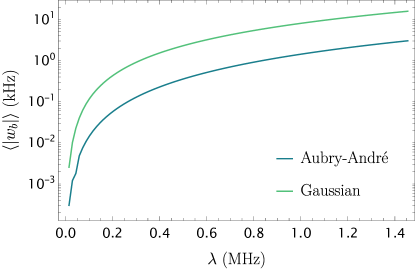
Figure 2: Random Gaussian disorder vs Metallic-Aubry-André: Exact diagonalization results for averaged Walsh-Hadamard coefficients as a function of the effective bare coupling $\lambda=16JE_{\text{C}}/\langle\omega\rangle$ for Metallic-Aubry-André and random Gaussian disorder with matching standard deviation. The averaging is done over Walsh-Hadamard coefficients of weight 2 and correlation range $\ell=1$ (nearest neighbor $ZZ$). For the case of the Gaussian random disorder there is additional averaging over 100 different realisations. The parameter values used here are $E_{\text{C}}=0.33\text{ GHz}$, $\langle\omega\rangle=5.5\text{ GHz}$, $\Delta=1\text{ GHz}$ and the coupling $J$ is varied over the range $0$ to $1.5\text{ MHz}$. The system size for both cases is $2\times 3$.

Results: The second order perturbation theory calculation for the qubit sector energy levels gives the following expressions for the first and second order corrections

$$E_{b} \simeq E_{\mu}b_{\mu}+E_{b}^{(1)}+E_{b}^{(2)},$$ (12a)

$$E_{b}^{(1)} =-E_{\text{C}}b_{\mu}b_{\mu}+\mathcal{E}^{\mu\nu}b_{\mu}b_{\nu},$$ (12b)

$$E_{b}^{(2)} =\mathcal{D}_{\alpha\beta}^{\mu\nu}b_{\mu}b_{\nu}1_{\alpha}1_{\beta}+(2\mathcal{D}_{\beta}^{\mu\nu\alpha}+\mathcal{S}_{\beta}^{\mu\nu\alpha})b_{\mu}b_{\nu}b_{\alpha}1_{\beta}.$$ (12c)

The explicit form and derivation of the tensors $\mathcal{E}$, $\mathcal{S}$ and $\mathcal{D}$ can be found in the supplemental material Eqs. (S16), (S33) and (S34) respectively, as well as an explanation of the index convention in Eq. (S17). Finally we used Einstein summation convention and $1_{\mu}$ denotes the $\mu$-th digit of the bit-string with all entries 1.

The energy denominators of perturbation theory are notoriously known to cause issues with accuracy, particularly when the involved basis states are resonant (i.e. when denominators are vanishing). Even though these denominators involve energy levels of the dressed basis, in the localised regime these are essentially indistinguishable from the bare basis energy levels $E_{\mu}=\omega(x_{\mu},y_{\mu})+O(J^{2}/\Delta)$. Therefore we can straightforwardly associate spatial coordinates $(x_{i},y_{i})$ on our lattice to them. From the form $\propto c_{\alpha}^{\dagger}c_{\beta}c_{\mu}^{\dagger}c_{\nu}$ of the perturbing potential in the dressed basis, it is clear that only states which are two hops apart can have a non vanishing amplitude. Thus the energy denominator can involve between 2, 3, or 4 different sites. The terms involving only 2 sites can be thought of as effectively single hops and are all included in $\mathcal{S}$. These resonances we will refer to as site resonances or simply resonances. The terms involving 3 or 4 sites can only be described as double hoping terms and are all included in $\mathcal{D}$. These resonances we will refer to as mode resonances.

With the introduction of the metallic ratio Aubry-André scheme, our motivation has been to set up a quasi-random disorder potential without resonances and with well separated near-resonant sites. However a direct implication of Eq. (12c), and specifically of the form of $\mathcal{D}_{\mu\nu\alpha\beta}\propto(E_{\mu}+E_{\nu}-E_{\alpha}-E_{\beta})^{-1}$, is that this consideration is not sufficient to successfully localize the system. Granted that having such a denominator vanishing or being much smaller than $E_{\text{C}}$ does not necessarily mean that our system is chaotic but it does suggest strong hybridization between certain modes which is certainly not desirable for quantum computation. While the denominator of $\mathcal{D}_{\mu\nu\alpha\beta}$ creates these dangers for perturbation theory, its numerators have a counteracting effect. They are proportional to the 4 point function $\langle\psi_{\mu}\psi_{\nu}\psi_{\alpha}\psi_{\beta}\rangle$ (cf. Eq. (S5)) of the single particle eigenvectors involving the same states as the ones in the denominator. Anderson localization theory shows that these correlations decay exponentially with range.

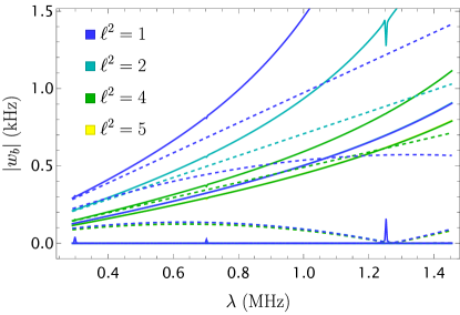
Figure 3: Exact diagonalization vs perturbation theory: Plots of all the Walsh-Hadamard coefficients of weight 2 as a function of the effective bare coupling $\lambda=16JE_{\text{C}}/\langle\omega\rangle$ using exact diagonalization (solid) and perturbation theory (dashed). Parameter values and system size are the same as the ones used in Fig. 2. Coefficients are color-coded with respect to the corresponding correlation range $\ell$ as indicated by the legend. The sharp spikes for the case of exact diagonalization are due to discontinuities in the qubit energy levels because of level anti-crossings.

From the analytical expressions for the energy levels we can immediately derive the Walsh-Hadamard coefficients with the use of the properties

$$\sum_{a=0}^{1}(-1)^{b\cdot\bar{a}}=2\bar{b}\quad\text{and}\quad\sum_{a=0}^{1}(-1)^{b\cdot\bar{a}}a=1$$ (13)

Due to the linearity of the Walsh-Hadamard transformation, we can apply it separately for each component Eqs. (12a)-(12c). Furthermore, the summation over all possible bit-strings can be recast into the form of multiple summations over each bit-digit like the ones in Eq. (13). Each term in the perturbative expressions for the energy levels has been purposefully written so that it clearly contains a specific number of different bit-digits. Therefore, a term containing $m$ bit digits will eliminate $m$ of the $N$ Walsh-Hadamard summations and the remaining summations will yield a product of the other $N-m$ flipped digits. Therefore if the Walsh-Hadamard coefficient corresponds to a bit-string of weight more than $m$ it will be vanishing. As a direct consequence of that, in conjunction with the form of Eqs. (12a)-(12c), first order perturbation theory can only yield corrections for Walsh-Hadamard coefficients up to weight 2 and second order perturbation theory up to weight 3. The exact form of these coefficients can be found in the suplemental material Eqs. (S47)-(S49). A further simplified version of these expressions can be derived by using Table S1, with the results reported in Table  S2.

Once we have selected the metallic Aubry-André model as our disorder potential our first goal is to establish how well it performs in terms of localizing our system compared to random disorder. We have performed this comparison for a smaller system of size $2\times 3$, which was manageable with exact diagonalization. The results are reported in Fig. 2 and confirm that our model outperforms random disorder of the same strength.

Our next goal is to obtain Walsh-Hadamard coefficients for a much larger system of dimensions $2\times 20$. Before doing that however we need to know the accuracy of our perturbation theory by comparing it with exact diagonalization results. For this comparison, still restricted to the $2\times 3$ system size, see Fig. 3. It is evident that the agreement of the two results is restricted to a rather small parameter range. Even though the second order perturbation theory is very accurate for the energy levels, with an error of $\sim 10^{-1}\text{ kHz}$ for eigenenergies spanning a few tens of GHz, the error is of the same order of magnitude as the Walsh-Hadamard coefficients of weight 2, and is about 2 orders of magnitude larger that coefficients of weight 3. This is why we only report the weight 2 coefficients here. Unfortunately the accuracy of the energy levels is not found to be improved by introducing higher order terms [26]; our perturbation theory is equivalent to that of the $\varphi^{4}$ theory, which is known to have a vanishing radius of convergence. Already at third order of perturbation theory the disagreement with the exact diagonalization results starts to increase.

Figure 4: Walsh-Hadamard exponential hierarchy: Plot of averaged Walsh-Hadamard coefficients of weight 2 as a function of the correlation range $\ell$ for a $2\times 20$ quasi-1D lattice. Averaging is done among Walsh-Hadamard coefficients of the same correlation range. The parameter values used here are $J=1\text{ MHz}$, $\langle\omega\rangle=5.5\text{ GHz}$, $\Delta=1\text{ GHz}$ and $E_{\text{C}}=0.15\text{ GHz}$. The inset is a visual representation of the relevant Walsh-Hadamard coefficient bit-strings for correlation range $\ell=1$ on the lattice. Blue corresponds to 0 and yellow to 1.

Despite these difficulties, we obtain meaningful results about the Walsh-Hadamard coefficients and the correct order of magnitude within the specified parameter range in Fig. 3. Therefore we deem it informative to obtain the weight 2 coefficients using perturbation theory for the much larger $2\times 20$ system, far beyond the size that is accessible by exact diagonarization. The results for this calculation are reported in Fig. 4. They confirm the expectation that these Walsh-Hadamard coefficients exhibit a hierarchy of values, decreasing exponentially with range; this is as expected within many body localization theory (see [9]).

Summary: We have demonstrated that it is possible to localize a many body quantum computing system without the use of random disorder but rather with a deterministically designed, nonperiodic potential. We believe that the disorder potential we studied here is not yet optimal and that meticulous frequency pattern engineering should play a crucial role in the design of future quantum computing architectures. Our new perturbation-theory scheme can be used as a guide for the properties a frequency pattern should possess or avoid. Despite the limited accuracy of our perturbation scheme, we have demonstrated that it is possible to obtain useful analytical results for the Walsh-Hadamard coefficients of large many-body systems. We believe that accuracy can ultimately be improved with a renormalized perturbation theory. Finally, we need to stress out that the results for the $2\times 20$ lattice are well beyond the realm of what is attainable with exact diagonalization techniques. The main impediment for increasing the size further is the exponential scaling of the number of Walsh-Hadamard coefficients themselves, which is $2^{N}$. However, if we instead restrict the calculation to only low-weight coefficients with small correlation range, then the main hurdle is the calculation of the tensors $\mathcal{S}$ and $\mathcal{D}$ which scale only polynomially with lattice size, but with a high power $\sim N^{4}$.

We acknowledge support from the Deutsche Forschungsgemeinschaft (DFG) under Germany’s Excellence Strategy Cluster of Excellence Matter and Light for Quantum Computing (ML4Q) EXC 2004/1 390534769.

I Supplement

Having obtained the eigenstates $|\psi_{\mu}\rangle$ of the single-particle sector of the Hamiltonian in Eq. (4) we can define the dressed basis ladder operators as

$$|\psi_{\mu}\rangle=\sum_{i=1}^{N}\psi_{\mu}(x_{i},y_{i})|x_{i},y_{i}\rangle=\left(\sum_{i=1}^{N}\psi_{\mu}(x_{i},y_{i})a_{i}^{\dagger}\right)|0\rangle\stackrel{{\scriptstyle!}}{{=}}c_{\mu}^{\dagger}|0\rangle,$$ (S1)

In the localised regime, the operators $c_{\mu}^{\dagger}$ can be thought of as the creation operators that create states localised around position $\mu$ of the lattice, in other words

$$c_{\mu}^{\dagger}=a_{\mu}^{\dagger}+O(J/\Delta).$$ (S2)

Using these conventions we can diagonalise our Hamiltonian as in Eq. (9).

In order to calculate the amplitudes appearing in the perturbative expansion of Eq. (7) we need to express the bare basis ladder operators in the dressed basis by inverting the transformation of Eq. (10). Using the completeness relation

$$\sum_{\mu=1}^{N}\psi_{\mu}(x_{i},y_{i})\psi_{\mu}^{*}(x_{j},y_{j})=\delta_{ij}$$ (S3)

we can obtain

$$\sum_{i=1}^{N}\psi_{\mu}(x_{i},y_{i})a_{i}^{\dagger}=c_{\mu}^{\dagger}\Rightarrow\sum_{\mu=1}^{N}\sum_{i=1}^{N}\psi_{\mu}(x_{i},y_{i})\psi_{\mu}^{*}(x_{j},y_{j})a_{i}^{\dagger}=\sum_{\mu=1}^{N}\psi_{\mu}^{*}(x_{j},y_{j})c_{\mu}^{\dagger}\Rightarrow a_{j}^{\dagger}=\sum_{\mu=1}^{L}\psi_{\mu}^{*}(x_{j},y_{j})c_{\mu}^{\dagger}$$ (S4)

and since our Hamiltonian is symmetric $\psi_{\mu}^{*}(x_{j},y_{j})=\psi_{\mu}(x_{j},y_{j})$. To lighten the notation we will denote the n-point correlation functions as

$$\sum_{i=1}^{N}\psi_{\mu_{1}}(x_{i},y_{i})\psi_{\mu_{2}}(x_{i},y_{i})\dots\psi_{\mu_{n}}(x_{i},y_{i})=\langle\psi_{\mu_{1}}\psi_{\mu_{2}}\dots\psi_{\mu_{n}}\rangle$$ (S5)

keeping in mind that Greek letters are dressed basis indices while Latin letters are bare basis indices. With these conventions we can express Eq. (7) as

$$E_{b}^{(1)}=-\frac{E_{\text{C}}}{2}\sum_{\alpha,\beta=1}^{N}\langle\psi_{\alpha}\psi_{\beta}\rangle\langle b|c_{\alpha}^{\dagger}c_{\beta}|b\rangle-\frac{E_{\text{C}}}{2}\sum_{\alpha,\beta,\mu,\nu=1}^{N}\langle\psi_{\alpha}\psi_{\beta}\psi_{\mu}\psi_{\nu}\rangle\langle b|c_{\alpha}^{\dagger}c_{\beta}c_{\mu}^{\dagger}c_{\nu}|b\rangle$$ (S6)

and we can now proceed to calculating the two relevant amplitudes. The first term is trivial since $\langle\psi_{\alpha}\psi_{\beta}\rangle=\delta_{\alpha\beta}$ is the orthonormality of the eigenstates and thus the amplitude is simply

$$\sum_{\alpha,\beta=1}^{N}\langle\psi_{\alpha}\psi_{\beta}\rangle\langle b|c_{\alpha}^{\dagger}c_{\beta}|b\rangle=\sum_{\alpha=1}^{N}\langle b|c_{\alpha}^{\dagger}c_{\alpha}|b\rangle=\sum_{\alpha=1}^{N}b_{\alpha}$$ (S7)

For the second term we can calculate the amplitude by use of Wick’s Theorem by expressing it as

$$\langle b|c_{\alpha}^{\dagger}c_{\beta}c_{\mu}^{\dagger}c_{\nu}|b\rangle=\langle 0|c_{N}^{b_{N}}\dots c_{2}^{b_{2}}c_{1}^{b_{1}}c_{\alpha}^{\dagger}c_{\beta}c_{\mu}^{\dagger}c_{\nu}(c_{1}^{\dagger})^{b_{1}}(c_{2}^{\dagger})^{b_{2}}\dots(c_{N}^{\dagger})^{b_{N}}|0\rangle$$ (S8)

and since any non fully contracted terms are normal ordered, only the fully contracted terms will contribute. With the contraction rules of Eq. (11) in mind, we can see that there is only one possible internal-internal (II) contraction between $c_{\beta}$ and $c_{\mu}^{\dagger}$ for which we obtain

$$\langle b|c_{\alpha}^{\dagger}c_{\beta}c_{\mu}^{\dagger}c_{\nu}|b\rangle_{\text{II}}=\sum_{\sigma=1}^{N}\delta_{\beta\mu}b_{\sigma}\delta_{\sigma\alpha}b_{\sigma}\delta_{\sigma\nu}=\delta_{\beta\mu}b_{\alpha}b_{\nu}\delta_{\alpha\nu}.$$ (S9)

and for the case with only internal-external (IE) contractions we have

$$\langle b|c_{\alpha}^{\dagger}c_{\beta}c_{\mu}^{\dagger}c_{\nu}|b\rangle_{\text{IE}} =\sum_{\sigma\neq\rho=1}^{N}b_{\sigma}\delta_{\sigma\alpha}b_{\rho}\delta_{\rho\mu}b_{\sigma}\delta_{\sigma\beta}b_{\rho}\delta_{\rho\nu}+\sum_{\sigma\neq\rho=1}^{N}b_{\sigma}\delta_{\sigma\alpha}b_{\rho}\delta_{\rho\mu}b_{\sigma}\delta_{\sigma\nu}b_{\rho}\delta_{\rho\beta}$$ (S10)

$$=b_{\alpha}b_{\beta}\delta_{\alpha\beta}b_{\mu}b_{\nu}\delta_{\mu\nu}+b_{\alpha}b_{\nu}\delta_{\alpha\nu}b_{\beta}b_{\mu}\delta_{\beta\mu}$$ (S11)

In total

$$\langle b|c_{\alpha}^{\dagger}c_{\beta}c_{\mu}^{\dagger}c_{\nu}|b\rangle=\langle b|c_{\alpha}^{\dagger}c_{\beta}c_{\mu}^{\dagger}c_{\nu}|b\rangle_{\text{IE}}+\langle b|c_{\alpha}^{\dagger}c_{\beta}c_{\mu}^{\dagger}c_{\nu}|b\rangle_{\text{II}}$$ (S12)

and the corresponding contribution in Eq. (S6) is

$$\sum_{\alpha,\beta,\mu,\nu=1}^{N}\langle\psi_{\alpha}\psi_{\beta}\psi_{\mu}\psi_{\nu}\rangle\langle b|c_{\alpha}^{\dagger}c_{\beta}c_{\mu}^{\dagger}c_{\nu}|b\rangle=2\sum_{\stackrel{{\scriptstyle\mu,\nu=1}}{{\mu\neq\nu}}}^{N}b_{\mu}^{2}b_{\nu}^{2}\langle\psi_{\mu}^{2}\psi_{\nu}^{2}\rangle+\sum_{\mu=1}^{N}b_{\mu}^{2}.$$ (S13)

Of course, $b_{\mu}\in\mathbb{B}$ thus the square is redundant and we can drop it. Substituting back into Eq. (S6) we obtain

$$E_{b}^{(1)}=-E_{\text{C}}\sum_{\mu=1}b_{\mu}-E_{\text{C}}\sum_{\stackrel{{\scriptstyle\mu,\nu=1}}{{\mu\neq\nu}}}^{N}b_{\mu}b_{\nu}\langle\psi_{\mu}^{2}\psi_{\nu}^{2}\rangle$$ (S14)

and therefore to first order approximation our energly levels will be

$$E_{b}\simeq E_{b}^{(0)}+E_{b}^{(1)}=\sum_{\mu=1}^{N}E_{\mu}b_{\mu}-E_{\text{C}}\sum_{\mu=1}^{N}b_{\mu}+E_{\text{C}}\sum_{\mu,\nu=1}^{N}\mathcal{E}^{\mu\nu}b_{\mu}b_{\nu}.$$ (S15)

where we introduced the matrix definition

$$\mathcal{E}_{\mu\nu}=-E_{\text{C}}\langle\psi_{\mu}^{2}\psi_{\nu}^{2}\rangle,$$ (S16)

and the index convention that no two upper indices can take the same value which can be expressed formally using the absolute value of the $n$-dimensional fully antisymmetric tensor $|\varepsilon_{i_{1}}\dots i_{n}|$ for an $m$ dimensional array $\mathcal{M}$

$$\mathcal{M}_{i_{n+1}\dots i_{m}}^{i_{1}\dots i_{n}}=\mathcal{M}_{i_{1}\dots i_{m}}|\varepsilon_{i_{1}\dots i_{n}}|.$$ (S17)

Finally, the zeroth order term $E_{b}^{(0)}$ is the expectation value of the Hamiltonian in Eq. (9) for the eigenstate Eq. (8).

We proceed with the second order perturbation theory term

$$E_{b}^{(2)}=\frac{E_{\text{C}}^{2}}{4}\sum_{m\neq b}\frac{|\sum_{x=1}^{N}\langle m|a_{x}^{\dagger}a_{x}|b\rangle+\sum_{x=1}^{N}\langle m|a_{x}^{\dagger}a_{x}a_{x}^{\dagger}a_{x}|b\rangle|^{2}}{E_{b}^{(0)}-E_{m}}.$$ (S18)

We now need to compute the two new amplitudes $\langle m|a_{x}^{\dagger}a_{x}|b\rangle$ and $\langle m|a_{x}^{\dagger}a_{x}a_{x}^{\dagger}a_{x}|b\rangle$ where the bra can be any Fock state, while the ket can only be a state of qubits (Fock indices 0 or 1). We transform the ladder operators in the dressed basis and write the first amplitude

$$\sum_{i=1}^{N}\langle m|a_{i}^{\dagger}a_{i}|b\rangle=\sum_{\alpha,\beta=1}^{N}\langle\psi_{\alpha}\psi_{\beta}\rangle\langle m|c_{\alpha}^{\dagger}c_{\beta}|b\rangle=\sum_{\alpha=1}^{N}\langle m|c_{\alpha}^{\dagger}c_{\alpha}|b\rangle=\langle m|b\rangle\sum_{\alpha=1}^{N}b_{\alpha}.$$ (S19)

In other words this amplitude only has diagonal elements and therefore does not contribute at all in second order of perturbation theory; thus

$$E_{b}^{(2)}=\frac{E_{\text{C}}^{2}}{4}\sum_{m\neq b}\frac{|\sum_{x=1}^{N}\langle m|a_{x}^{\dagger}a_{x}a_{x}^{\dagger}a_{x}|b\rangle|^{2}}{E_{b}^{(0)}-E_{m}}.$$ (S20)

For the remaining amplitude we will have

$$\sum_{x=1}^{N}\langle m|a_{x}^{\dagger}a_{x}a_{x}^{\dagger}a_{x}|b\rangle =\sum_{\mu_{i}=1}^{N}\langle\psi_{\mu_{1}}\psi_{\mu_{2}}\psi_{\mu_{3}}\psi_{\mu_{4}}\rangle\langle m|c_{\mu_{1}}^{\dagger}c_{\mu_{2}}c_{\mu_{3}}^{\dagger}c_{\mu_{4}}|b\rangle.$$ (S21)

We can define the vector

$$|\tilde{b}_{\mu_{1},\mu_{2},\mu_{3},\mu_{4}}\rangle=c_{\mu_{1}}^{\dagger}c_{\mu_{2}}c_{\mu_{3}}^{\dagger}c_{\mu_{4}}|b\rangle=|\tilde{b}_{\mu_{1},\mu_{2},\mu_{3},\mu_{4}}|\cdot|\hat{b}_{\mu_{1},\mu_{2},\mu_{3},\mu_{4}}\rangle$$ (S22)

(introducing the normalized vector $(|\hat{b}_{\mu_{1},\mu_{2},\mu_{3},\mu_{4}}\rangle$) so that

$$\sum_{x=1}^{N}\langle m|a_{x}^{\dagger}a_{x}a_{x}^{\dagger}a_{x}|b\rangle=\sum_{\mu_{i}=1}^{N}\langle\psi_{\mu_{1}}\psi_{\mu_{2}}\psi_{\mu_{3}}\psi_{\mu_{4}}\rangle\cdot|\tilde{b}_{\mu_{1},\mu_{2},\mu_{3},\mu_{4}}|\cdot\langle m|\hat{b}_{\mu_{1},\mu_{2},\mu_{3},\mu_{4}}\rangle.$$ (S23)

In order to lighten the notation we introduce the vector indices

$$\bm{\mu}=(\mu_{1},\mu_{2},\mu_{3},\mu_{4})$$ (S24)

and the multi-dimensional array

$$\Psi_{\bm{\mu}}=\langle\psi_{\mu_{1}}\psi_{\mu_{2}}\psi_{\mu_{3}}\psi_{\mu_{4}}\rangle$$ (S25)

to write

$$\sum_{x=1}^{N}\langle m|a_{x}^{\dagger}a_{x}a_{x}^{\dagger}a_{x}|b\rangle=\sum_{\bm{\mu}}\Psi_{\bm{\mu}}|\tilde{b}_{\bm{\mu}}|\delta_{m,\hat{b}_{\bm{\mu}}}$$ (S26)

and therefore for the second order energy correction we have

$$E_{b}^{(2)} =\frac{E_{\text{C}}^{2}}{4}\sum_{m\neq b}\frac{\sum_{\bm{\mu},\bm{\nu}}\Psi_{\bm{\mu}}\Psi_{\bm{\nu}}|\tilde{b}_{\bm{\mu}}||\tilde{b}_{\bm{\nu}}|\delta_{m,\hat{b}_{\bm{\mu}}}\delta_{m,\hat{b}_{\bm{\nu}}}}{E_{b}^{(0)}-E_{m}^{(0)}}$$ (S27)

$$=\frac{E_{\text{C}}^{2}}{4}\sum_{\stackrel{{\scriptstyle\bm{\mu},\bm{\nu}}}{{\hat{b}_{\bm{\mu}}\neq b}}}\frac{\Psi_{\bm{\mu}}\Psi_{\bm{\nu}}|\tilde{b}_{\bm{\mu}}||\tilde{b}_{\bm{\nu}}|\delta_{\hat{b}_{\bm{\mu}},\hat{b}_{\bm{\nu}}}}{E_{b}^{(0)}-E_{\hat{b}_{\bm{\mu}}}^{(0)}}$$ (S28)

$$=\frac{E_{\text{C}}^{2}}{4}\sum_{\stackrel{{\scriptstyle\bm{\mu},\bm{\nu}}}{{\hat{b}_{\bm{\mu}}\neq b}}}\frac{\Psi_{\bm{\mu}}\Psi_{\bm{\nu}}\langle\tilde{b}_{\bm{\mu}}|\tilde{b}_{\bm{\nu}}\rangle}{\Delta E_{\bm{\mu}}}$$ (S29)

with

$$\Delta E_{\bm{\mu}}=E_{b}^{(0)}-E_{\hat{b}_{\bm{\mu}}}^{(0)}=E_{b}^{(0)}-(E_{b}^{(0)}-E_{\mu_{1}}+E_{\mu_{2}}-E_{\mu_{3}}+E_{\mu_{4}})=E_{\mu_{1}}+E_{\mu_{3}}-E_{\mu_{2}}-E_{\mu_{4}}.$$ (S30)

Note here that $|\hat{b}_{\bm{\mu}}\rangle=|\hat{b}_{\bm{\nu}}\rangle$ does not guarantee $\bm{\mu}=\bm{\nu}$, in fact there may be several permutations of $\bm{\mu}$ ($\bm{\nu}$) that yield the same state but with different norm $|\tilde{b}_{\bm{\mu}}|$($|\tilde{b}_{\bm{\nu}}|$). We now have to calculate the amplitude

$$\langle\tilde{b}_{\bm{\mu}}|\tilde{b}_{\bm{\nu}}\rangle=\langle b|c_{\mu_{1}}^{\dagger}c_{\mu_{2}}c_{\mu_{3}}^{\dagger}c_{\mu_{4}}c_{\nu_{1}}^{\dagger}c_{\nu_{2}}c_{\nu_{3}}^{\dagger}c_{\nu_{4}}|b\rangle=\langle 0|c_{1}^{b_{1}}\dots c_{N}^{b_{N}}c_{\mu_{1}}^{\dagger}c_{\mu_{2}}c_{\mu_{3}}^{\dagger}c_{\mu_{4}}c_{\nu_{1}}^{\dagger}c_{\nu_{2}}c_{\nu_{3}}^{\dagger}c_{\nu_{4}}(c_{1}^{\dagger})^{b_{1}}\dots(c_{N}^{\dagger})^{b_{N}}|0\rangle.$$ (S31)

After calculating this vacuum expectation value by means of the Wick contractions and substituting into the energy correction we obtain

$$E_{b}^{(2)}=\sum_{\alpha,\beta,\mu,\nu=1}^{N}\left[\mathcal{D}_{\mu\nu}^{\alpha\beta}b_{\alpha}b_{\beta}+(2\mathcal{D}_{\nu}^{\alpha\beta\mu}+\mathcal{S}_{\nu}^{\alpha\beta\mu})b_{\alpha}b_{\beta}b_{\mu}+(\mathcal{D}^{\alpha\beta\mu\nu}+\mathcal{S}^{\alpha\beta\mu\nu})b_{\alpha}b_{\beta}b_{\mu}b_{\nu}\right]$$ (S32)

where we used the notation of Eq. (S17) and introduced the new multi-dimensional arrays

$$\mathcal{S}_{\alpha\beta\mu\nu} =\begin{cases}\displaystyle{4E_{\text{C}}^{2}\frac{\langle\psi_{\alpha}^{2}\psi_{\mu}\psi_{\nu}\rangle\langle\psi_{\beta}^{2}\psi_{\mu}\psi_{\nu}\rangle}{E_{\mu}-E_{\nu}},}&\mu\neq\nu\\ \displaystyle{0,}&\mu=\nu\end{cases}$$ (S33)

$$\mathcal{D}_{\alpha\beta\mu\nu} =\begin{cases}\displaystyle{E_{\text{C}}^{2}\frac{\langle\psi_{\alpha}\psi_{\beta}\psi_{\mu}\psi_{\nu}\rangle^{2}}{E_{\alpha}+E_{\beta}-E_{\mu}-E_{\nu}},}&\{\alpha,\beta\}\neq\{\mu,\nu\}\\ \displaystyle{0,}&\{\alpha,\beta\}=\{\mu,\nu\}.\end{cases}$$ (S34)

In the second case, the notation $\{\dots\}\neq\{\dots\}$ refers to set inequality, meaning that the vector $(\alpha,\beta)^{T}$ is not equal to the vector $(\mu,\nu)^{T}$ or to the vector $(\nu,\mu)^{T}$. At this point it will prove beneficial to consider the symmetry properties of these tensors, derived immediately from Eqs. (S34) and (S33)

$$\mathcal{S}_{\alpha\beta\mu\nu}=\mathcal{S}_{\beta\alpha\mu\nu}=-\mathcal{S}_{\alpha\beta\nu\mu},$$ (S35)

$$\mathcal{D}_{\alpha\beta\mu\nu}=\mathcal{D}_{\beta\alpha\mu\nu}=\mathcal{D}_{\alpha\beta\nu\mu}=-\mathcal{D}_{\mu\nu\alpha\beta},$$ (S36)

$$\mathcal{S}_{\alpha\alpha\beta\nu}=4\mathcal{D}_{\alpha\beta\alpha\nu}.$$ (S37)

From these we can already see that the last term in Eq. (S32) is vanishing, so that

$$E_{b}^{(2)}=\sum_{\alpha,\beta,\mu,\nu=1}^{N}\left[\mathcal{D}_{\mu\nu}^{\alpha\beta}b_{\alpha}b_{\beta}+(2\mathcal{D}_{\nu}^{\alpha\beta\mu}+\mathcal{S}_{\nu}^{\alpha\beta\mu})b_{\alpha}b_{\beta}b_{\mu}\right]$$ (S38)

Using the linearity of the Walsh-Hadamard transformation (see Eq. (2) of the main text) we can calculate

$$w_{b} =\frac{1}{2^{N}}\sum_{a\in\mathbb{B}^{N}}(-1)^{b\cdot\bar{a}}E_{a}$$ (S39)

$$\simeq\frac{1}{2^{N}}\sum_{a\in\mathbb{B}^{N}}(-1)^{b\cdot\bar{a}}E_{a}^{(0)}+\frac{1}{2^{N}}\sum_{a\in\mathbb{B}^{N}}(-1)^{b\cdot\bar{a}}E_{a}^{(1)}+\frac{1}{2^{N}}\sum_{a\in\mathbb{B}^{N}}(-1)^{b\cdot\bar{a}}E_{a}^{(2)}$$ (S40)

$$=w_{b}^{(0)}+w_{b}^{(1)}+w_{b}^{(2)}.$$ (S41)

As it turns out, with second order perturbation theory, one obtains contributions to the Walsh-Hadamard coefficients up to weight 3, while higher weight coefficients are analytically vanishing. We will prove this now, starting from

$$w_{b}^{(0)} =\frac{1}{2^{N}}\sum_{\mu=1}^{N}E_{\mu}\sum_{a\in\mathbb{B}^{N}}(-1)^{b\cdot\bar{a}}a_{\mu}$$ (S42)

$$w_{b}^{(1)} =\frac{1}{2^{N}}\sum_{\mu,\nu=1}^{N}\mathcal{E}_{\mu\nu}\sum_{a\in\mathbb{B}^{N}}(-1)^{b\cdot\bar{a}}a_{\mu}a_{\nu}-\frac{E_{\text{C}}}{2^{N}}\sum_{\mu=1}^{N}\sum_{a\in\mathbb{B}^{N}}(-1)^{b\cdot\bar{a}}a_{\mu}$$ (S43)

$$w_{b}^{(2)} =\frac{1}{2^{N}}\sum_{\mu,\nu,\alpha,\beta=1}^{N}\mathcal{D}_{\alpha\beta}^{\mu\nu}\sum_{a\in\mathbb{B}^{N}}(-1)^{b\cdot\bar{a}}a_{\mu}a_{\nu}+\frac{1}{2^{N}}\sum_{\mu,\nu,\alpha,\beta=1}^{N}(2\mathcal{D}_{\beta}^{\mu\nu\alpha}+\mathcal{S}_{\beta}^{\mu\nu\alpha})\sum_{a\in\mathbb{B}^{N}}(-1)^{b\cdot\bar{a}}a_{\mu}a_{\nu}a_{\alpha}.$$ (S44)

Using the relations Eq. (13) we can perform the Boolean summations

$$\frac{1}{2^{N}}\sum_{a\in\mathbb{B}^{N}}(-1)^{b\cdot\bar{a}}a_{\mu_{1}}\dots a_{\mu_{m}} =\frac{1}{2^{N}}\left(\sum_{a_{1}=0}^{1}(-1)^{b_{1}\bar{a}_{1}}\right)\dots\left(\sum_{a_{\mu_{1}}=0}^{1}(-1)^{b_{\mu_{1}}\bar{a}_{\mu_{1}}}a_{\mu_{1}}\right)\dots\left(\sum_{a_{N}=0}^{1}(-1)^{b_{N}\bar{a}_{N}}\right)$$ (S45)

$$=\frac{1}{2^{m}}\prod_{\stackrel{{\scriptstyle i=1}}{{i\neq\mu_{1},\dots,\mu_{m}}}}^{N}\bar{b}_{i}$$ (S46)

and therefore

$$w_{b}^{(0)} =\frac{1}{2}\sum_{\mu=1}^{N}E_{\mu}\prod_{\stackrel{{\scriptstyle i=1}}{{i\neq\mu}}}^{N}\bar{b}_{i}$$ (S47)

$$w_{b}^{(1)} =\frac{1}{4}\sum_{\mu,\nu=1}^{N}\mathcal{E}_{\mu\nu}\prod_{\stackrel{{\scriptstyle i=1}}{{i\neq\mu,\nu}}}^{N}\bar{b}_{i}-\frac{E_{\text{C}}}{2}\sum_{\mu=1}^{N}\prod_{\stackrel{{\scriptstyle i=1}}{{i\neq\mu}}}^{N}\bar{b}_{i}$$ (S48)

$$w_{b}^{(2)} =\frac{1}{4}\sum_{\mu,\nu,\alpha,\beta=1}^{N}\mathcal{D}_{\mu\nu\alpha\beta}|\varepsilon_{\mu\nu}|\prod_{\stackrel{{\scriptstyle i=1}}{{i\neq\mu,\nu}}}^{N}\bar{b}_{i}+\frac{1}{8}\sum_{\mu,\nu,\alpha,\beta=1}^{N}(2\mathcal{D}_{\mu\nu\alpha\beta}+\mathcal{S}_{\mu\nu\alpha\beta})|\varepsilon_{\mu\nu\alpha}|\prod_{\stackrel{{\scriptstyle i=1}}{{i\neq\mu,\nu,\alpha}}}^{N}\bar{b}_{i}$$ (S49)

In order to complete the calculation of the Walsh-Hadamard coefficients we now need to consider the values of the flipped bit digit products and eliminate the absolute values of the fully antisymmetric tensor that appear in these expressions. We start with the products. These are, generally, products of the $N$ flipped digits of bit-string $b$ excluding $m$ of them. The only way for such a product to not be vanishing is if all the digits of bit-string $b$ except $m$ of them are all 0. The excluded ones can however be either 0 or 1. In other words, $b$ can only be weight $m$ or smaller. Since the highest value of $m$ up to second order is 3, we have vanishing Walsh-Hadamard coefficients of weight higher than 4. We summarised the values of these products for the various cases of Walsh-Hadamard weights 0 to 3 in Table S1.

Finally the absolute value of the fully anti-symmetric tensor can be eliminated using a combination of the symmetries of $\mathcal{S}$ and $\mathcal{D}$ as well as the properties:

$$f_{\alpha\beta\mu\nu}|\varepsilon_{\alpha\beta}|=f_{\alpha\beta\mu\nu}-f_{\alpha\alpha\mu\nu}\delta_{\alpha\beta},$$ (S50)

$$f_{\alpha\beta\mu\nu}|\varepsilon_{\alpha\beta\mu}|=f_{\alpha\beta\mu\nu}+2f_{\alpha\alpha\alpha\nu}\delta_{\alpha\beta}\delta_{\beta\mu}-f_{\alpha\alpha\mu\nu}\delta_{\alpha\beta}-f_{\alpha\beta\alpha\nu}\delta_{\alpha\mu}-f_{\alpha\beta\beta\nu}\delta_{\beta\mu}.$$ (S51)

with $f$ some arbitrary multi-dimensional array. The final results are reported in Table S2.

$m$	$\displaystyle{\prod_{\stackrel{{\scriptstyle i=1}}{{i\neq\mu}}}^{N}\bar{b}_{i}}$	$\displaystyle{\prod_{\stackrel{{\scriptstyle i=1}}{{i\neq\mu,\nu}}}^{N}\bar{b}_{i}}$	$\displaystyle{\prod_{\stackrel{{\scriptstyle i=1}}{{i\neq\mu,\nu,\alpha}}}^{N}\bar{b}_{i}}$
$0$	$1$	$1$	$1$
1	$\delta_{\mu\ell_{1}}$	$\delta_{\mu\ell_{1}}+\delta_{\nu\ell_{1}}$	$\delta_{\mu\ell_{1}}+\delta_{\nu\ell_{1}}+\delta_{\alpha\ell_{1}}$
2	$0$	$\delta_{\mu\ell_{1}}\delta_{\nu\ell_{2}}+\delta_{\nu\ell_{1}}\delta_{\mu\ell_{2}}$	$\delta_{\mu\ell_{1}}\delta_{\nu\ell_{2}}+\delta_{\mu\ell_{2}}\delta_{\nu\ell_{1}}+\delta_{\nu\ell_{2}}\delta_{\alpha\ell_{1}}+\delta_{\mu\ell_{1}}\delta_{\alpha\ell_{2}}+\delta_{\mu\ell_{2}}\delta_{\alpha\ell_{1}}+\delta_{\nu\ell_{1}}\delta_{\alpha\ell_{2}}$
3	$0$	$0$	$\delta_{\mu\ell_{1}}\delta_{\nu\ell_{2}}\delta_{\alpha\ell_{3}}+\delta_{\mu\ell_{2}}\delta_{\nu\ell_{1}}\delta_{\alpha\ell_{3}}+\delta_{\mu\ell_{3}}\delta_{\nu\ell_{2}}\delta_{\alpha\ell_{1}}+\delta_{\mu\ell_{1}}\delta_{\nu\ell_{3}}\delta_{\alpha\ell_{2}}+\delta_{\mu\ell_{2}}\delta_{\nu\ell_{3}}\delta_{\alpha\ell_{1}}+\delta_{\mu\ell_{3}}\delta_{\nu\ell_{1}}\delta_{\alpha\ell_{2}}$

Table S1: Flipped bit-digit products: Summary of all possible combinations for bit digit products. $m$, the Walsh-Hadamard weight, changes vertically from 0 to 3 and number of excluded bit digits changes horizontally from 1 to 3. In the notation employed here, a bit-string of weight $m$ has 1’s at positions $\ell_{1},\dots,\ell_{m}$.

$m$	$n=0$	$n=1$	$n=2$
0	$\frac{1}{2}\sum_{\mu}E_{\mu}$	$\frac{1}{4}\sum_{\mu,\nu}\mathcal{E}_{\mu\nu}-N\frac{E_{\text{C}}}{2}$	$\frac{1}{2}\sum_{\mu,\nu,\alpha}\mathcal{D}_{\mu\nu\alpha\alpha}+\frac{3}{2}\sum_{\nu,\alpha}\mathcal{D}_{\alpha\alpha\alpha\nu}$
1	$\frac{1}{2}E_{\ell_{1}}$	$\frac{1}{2}\sum_{\mu}\mathcal{E}_{\mu\ell_{1}}-\frac{E_{\text{C}}}{2}$	$\sum_{\mu,\nu,\beta}\left[\frac{3}{4}\mathcal{D}_{\ell_{1}\beta\mu\nu}+\frac{1}{8}\mathcal{S}_{\beta\mu\ell_{1}\nu}\right]+\sum_{\mu,\nu}\left[\mathcal{D}_{\mu\nu\ell_{1}\ell_{1}}+\frac{1}{4}\mathcal{D}_{\ell_{1}\nu\mu\mu}+\frac{1}{4}\mathcal{S}_{\ell_{1}\mu\nu\mu}\right]+\frac{9}{2}\sum_{\nu}\mathcal{D}_{\ell_{1}\ell_{1}\ell_{1}\nu}$
2	$0$	$\frac{1}{2}\mathcal{E}_{\ell_{1}\ell_{2}}$	$\sum_{\mu,\nu}\mathcal{D}_{\ell_{1}\ell_{2}\mu\nu}-\sum_{\nu}\left[2\mathcal{D}_{\ell_{1}\ell_{2}\ell_{1}\nu}+2\mathcal{D}_{\ell_{1}\ell_{2}\ell_{2}\nu}+\frac{1}{2}\mathcal{D}_{\ell_{1}\ell_{1}\ell_{2}\nu}+\frac{1}{2}\mathcal{D}_{\ell_{2}\ell_{2}\ell_{1}\nu}+\frac{1}{2}\mathcal{S}_{\ell_{1}\ell_{2}\ell_{1}\nu}+\frac{1}{2}\mathcal{S}_{\ell_{1}\ell_{2}\ell_{2}\nu}\right]$
3	$0$	$0$	$\sum_{\nu}\left[\frac{1}{2}\mathcal{D}_{\ell_{1}\ell_{2}\ell_{3}\nu}+\frac{1}{2}\mathcal{D}_{\ell_{1}\ell_{3}\ell_{2}\nu}+\frac{1}{2}\mathcal{D}_{\ell_{2}\ell_{3}\ell_{1}\nu}+\frac{1}{4}\mathcal{S}_{\ell_{1}\ell_{2}\ell_{3}\nu}+\frac{1}{4}\mathcal{S}_{\ell_{1}\ell_{3}\ell_{2}\nu}+\frac{1}{4}\mathcal{S}_{\ell_{2}\ell_{3}\ell_{1}\nu}\right]$

Table S2: Walsh-Hadamard formulae: Analytic expressions for the $n$-th order correction of Walsh-Hadamard coefficients of weight $m$ $w_{\ell_{1}\dots\ell_{m}}^{(n)}$. The convention for the position of 1’s in bit-string $b$ is the same as the one used in Table  S1. Each summation index runs over the entire range $\left[1,N\right]$.

References

Arute et al. [2019]F. Arute, K. Arya,
R. Babbush, D. Bacon, J. C. Bardin, R. Barends, R. Biswas, S. Boixo, F. G. Brandao, D. A. Buell, et al., Nature 574, 505 (2019).
Wu et al. [2021]Y. Wu, W.-S. Bao,
S. Cao, F. Chen, M.-C. Chen, X. Chen, T.-H. Chung, H. Deng, Y. Du, D. Fan, M. Gong, C. Guo, C. Guo, S. Guo, L. Han, L. Hong, H.-L. Huang, Y.-H. Huo, L. Li, N. Li, S. Li, Y. Li, F. Liang, C. Lin, J. Lin, H. Qian, D. Qiao, H. Rong, H. Su, L. Sun, L. Wang, S. Wang, D. Wu, Y. Xu, K. Yan, W. Yang, Y. Yang, Y. Ye, J. Yin, C. Ying, J. Yu, C. Zha, C. Zhang, H. Zhang, K. Zhang, Y. Zhang, H. Zhao, Y. Zhao, L. Zhou, Q. Zhu, C.-Y. Lu, C.-Z. Peng, X. Zhu, and J.-W. Pan, Phys. Rev. Lett. 127, 180501 (2021).
DiCarlo et al. [2009]L. DiCarlo, J. M. Chow,
J. M. Gambetta, L. S. Bishop, B. R. Johnson, D. Schuster, J. Majer, A. Blais, L. Frunzio, S. Girvin, et al., Nature 460, 240 (2009).
Yan et al. [2018]F. Yan, P. Krantz,
Y. Sung, M. Kjaergaard, D. L. Campbell, T. P. Orlando, S. Gustavsson, and W. D. Oliver, Phys. Rev. Applied 10, 054062 (2018).
Ku et al. [2020]J. Ku, X. Xu, M. Brink, D. C. McKay, J. B. Hertzberg, M. H. Ansari, and B. L. T. Plourde, Phys. Rev. Lett. 125, 200504 (2020).
Hertzberg et al. [2021]J. B. Hertzberg, E. J. Zhang, S. Rosenblatt,
E. Magesan, J. A. Smolin, J.-B. Yau, V. P. Adiga, M. Sandberg, M. Brink, J. M. Chow, et al., npj Quantum Information 7, 1 (2021).
Note [1]The reason for this bit flipping is the unfortunate
convention in quantum information of having the ground state denoted by 1 and
the first excited by 0, which we do not adopt here.
Koch et al. [2007]J. Koch, T. M. Yu,
J. Gambetta, A. A. Houck, D. I. Schuster, J. Majer, A. Blais, M. H. Devoret, S. M. Girvin, and R. J. Schoelkopf, Phys. Rev. A 76, 042319 (2007).
Roati et al. [2008]G. Roati, C. D’Errico,
L. Fallani, M. Fattori, C. Fort, M. Zaccanti, G. Modugno, M. Modugno, and M. Inguscio, Nature 453, 895 (2008).