Optimal Control Design for Operating a Hybrid PV Plant with Robust Power Reserves for Fast Frequency Regulation Services

Abstract

This paper presents an optimal control strategy for operating a solar hybrid system consisting of solar photovoltaic (PV) and a high-power, low-storage battery energy storage system (BESS). A state-space model of the hybrid PV plant is first derived, based on which an adaptive model predictive controller is designed. The controller’s objective is to control the PV and BESS to follow power setpoints sent to the the hybrid system while maintaining desired power reserves and meeting system operational contraints. Furthermore, an extended Kalman filter (EKF) is implemented for estimating the battery SOC, and an error sensitivity is executed to assess its limitations. To validate the proposed strategy, detailed EMT models of the hybrid system are developed so that losses and control limits can be quantified accurately. Day-long simulations are performed in an OPAL-RT real-time simulator using second-by-second actual PV farm data as inputs. Results verify that the proposed method can follow power setpoints while maintaining power reserves in days of high irradiance intermittency even with a small BESS storage.

I Introduction

The penetration of inverter-based resources (IBRs) is expected to increase sharply in many regional grids, and as conventional synchronous machines are substituted by IBRs, the grid’s inertia will drastically reduce in the upcoming years. For instance, in [1], Yuan et al. estimated a 1% system inertia reduction for every 1% increase in the photovoltaic (PV) penetration for the WECC system. This inertia decline leads to higher rate-of-change-of-frequency (ROCOF) and more severe frequency nadirs during contingencies, which may trigger under-frequency-load shedding and even the cascading tripping of generating units. To counter the aforementioned issues, new grid standards [2][3] have raised requirements for IBRs to provide grid support functions (GSFs), such as power curtailment, stronger disturbance ride-through characteristics, and response to high ROCOF events.

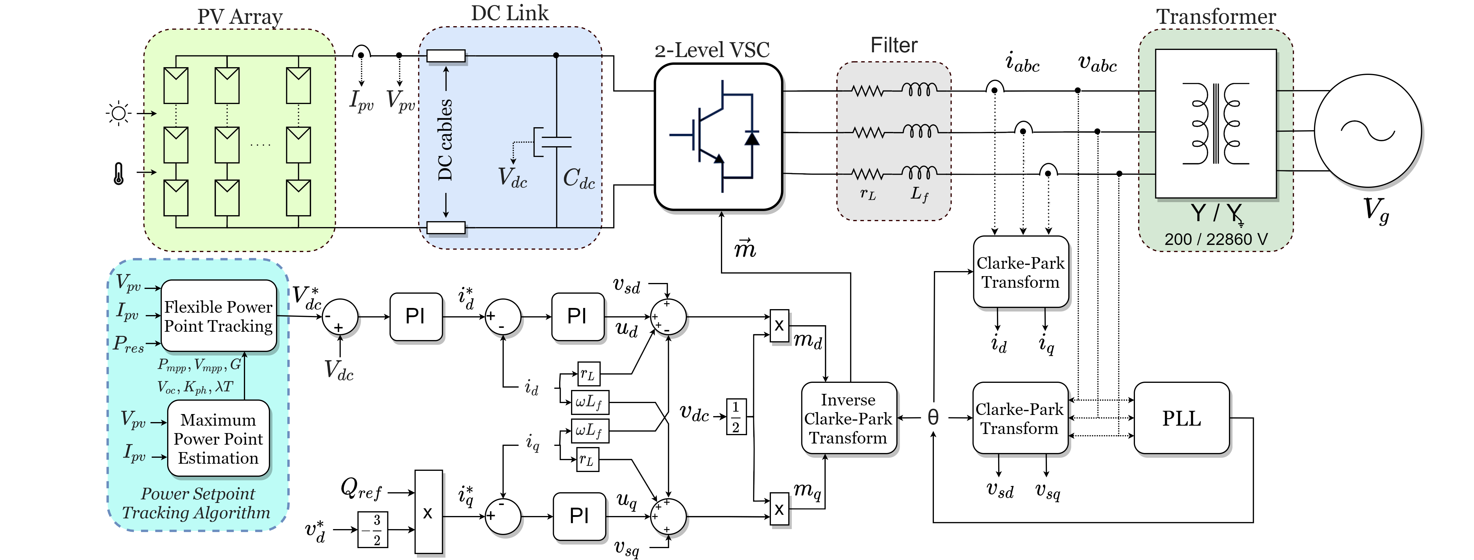
Figure 1: Circuit and control system block diagrams of a utility-scale PV system.

In [4], we introduced a PV power curtailment algorithm for maintaining accurate power reserves and providing fast frequency response (FFR) services to achieve higher frequency nadirs during contingencies. However, PV farms, operating by themselves, are still susceptible to fast clouding events. When irradiance drops sharply, even though a headroom is left for providing frequency support, the power reserves will quickly diminish, and consequently either the reserves or the power output will have to reduce. Therefore, using advanced power curtailment strategies alone cannot guarantee a PV plant to provide robust power reserves and follow power setpoints simultaneously under all weather conditions.

To provide robust power reserves, it is necessary for a PV plant to be coordinated with other resources. In [5], Chang et al. propose a coordination among multiple PV plants located in different geographic locations, so that if a shading event is imminent, power reserves are preemptively built up in other plants to help minimize the transient. Nevertheless, the approach is complicated, requiring coordination and communication among many PV plants, and by changing the PV injection in different regions, the system may experience voltage control issues due to PV injection variation.

A promising approach is to form hybrid PV plants so that grid-following battery energy storage systems (BESS) can be dispatched for enhancing the capability of PV plants to follow power setpoints and/or maintain headrooms at all times. One advantage of this approach is that the BESS can also be used to blackstart the PV plant [6] during blackouts. In [7], Teleke et al. proposed the usage of state-of-charge (SOC) feedback strategy when integrating the BESS into a wind farm, whereas in [8], Daud et al. apply the same strategy to a PV plant without the power curtailment functionality. In [9], Teleke et al. improved their performance by substituting the SOC feedback strategy with optimal control techniques. Advantages of the optimal control approach (e.g., model predictive control (MPC)) include considering future changes in the control objective, accounting for inputs and outputs constraints, and robustness to modeling errors due to its inherent feedback control characteristic [10].

Until now, an uncharted area is the control of intra-minute PV and BESS power outputs for meeting the reserve requirement and providing FFR. In [11], Nair et al. propose an MPC based algorithm for regulating PV and BESS in an energy scheduling problem with a step size of 5 minutes, which cannot deal with the intra-minute PV power fluctuations. In [12], Lei et al. present the coordination of PV and BESS via optimal control in a smaller time scale, but the work is not focused on day-long operation and does not consider PV power reserves. BESS and PV intra-minute power coordination with detailed models is presented by Chen et al. in [13], which is a rule-based algorithm (not optimal) and does not account for PV curtailment or power reserves. Another drawback of the existing approaches is that most works use simplified BESS and/or PV models, which are insufficient for assessing the dynamic performance when providing fast grid services.

Therefore, in this paper, we propose an optimal control strategy for operating a hybrid PV plant to provide reserves for regulation and FFR. The PV plant is equipped with the power curtailment algorithm recently introduced in [4] for tracking power setpoints and maximum power point estimation (MPPE) under fast irradiance intermittency. A detailed lithium-ion battery model that has been experimentally validated in the literature is implemented for a more realistic approach, and an extended Kalman filter (EKF) is designed for estimating the battery SOC. Detailed EMT models for both the PV and the grid-following BESS units are developed in a real-time simulator from OPAL-RT. Day-long simulations with high resolution irradiance and temperature data collected by our industry partner, Strata Solar, are executed to analyze the capability of the hybrid PV plant to maintain power reserves while following a regulation D signal from PJM.

The main contributions of the work to the literature are two-fold. First, we develop an optimal control strategy for operating a hybrid PV plant that can maintain robust power reserves for regulation and/or FFR services. Second, we derive a state-space (SS) model for the hybrid PV plant composed by an utility-scale PV system, a grid-following BESS unit, and an accurate second-order lithium-ion battery model. The proposed model is validated by day-long simulations using realistic data sets and detailed EMT models of the PV Plant and BESS.

II Methodology

II-A PV Plant Model

As shown in Fig. 1, the control system of the utility-scale PV plant uses a hierarchical control structure composed of a dc-link voltage controller cascaded with a current controller used to generate the inverter modulation signal, $\vec{m}$. More details on the converter controller can be found in [14]. The PV array model shown in Fig. 2 is described by

$$I_{\mathrm{pv}}=I_{\mathrm{ph}}-I_{\mathrm{s}}\Big{(}e^{\frac{V_{\mathrm{pv}}+I_{\mathrm{pv}}R_{\mathrm{s}}}{a}}-1\Big{)}-\Big{(}\frac{V_{\mathrm{pv}}+I_{\mathrm{pv}}R_{\mathrm{s}}}{R_{\mathrm{sh}}}\Big{)}$$ (1)

$$V_{\mathrm{mp}}=\bigg{(}1+\frac{R_{\mathrm{s}}}{R_{\mathrm{sh}}}\bigg{)}a(w-1)-R_{\mathrm{s}}I_{\mathrm{ph}}\bigg{(}1-\frac{1}{w}\bigg{)}$$ (2)

$$I_{\mathrm{mp}}=I_{\mathrm{ph}}\bigg{(}1-\frac{1}{w}\bigg{)}-\frac{a(w-1)}{R_{\mathrm{sh}}}$$ (3)

$$P_{\mathrm{mp}}=V_{\mathrm{mp}}I_{\mathrm{mp}}$$ (4)

$$w=W\bigg{\{}I_{\mathrm{ph}}\frac{e}{I_{\mathrm{s}}}\bigg{\}}$$ (5)

where $a$ is an ideality factor; $R_{\mathrm{s}}$ and $R_{\mathrm{sh}}$ are the series and shunt resistances, respectively; $I_{\mathrm{ph}}$ and $I_{\mathrm{s}}$ are the photo and diode saturation currents, respectively; and $w$, given by (5), is calculated with the Lambert $W$ function. The EMT models and the non-linear least squares Levenberg-Marquardt technique utilized for the MPPE are discussed in detail in [4] and [15].

Figure 2: Single-diode PV model circuit.

II-B Grid-Following BESS Model

The BESS unit, displayed in Fig. 3, consists of (i) a lithium-ion battery, (ii) a three-phase inverter operating in grid-following mode, (iii) an LC output filter, and (iv) an output Y-Yg transformer. Figure 3 displays the BESS circuit and control system diagram.

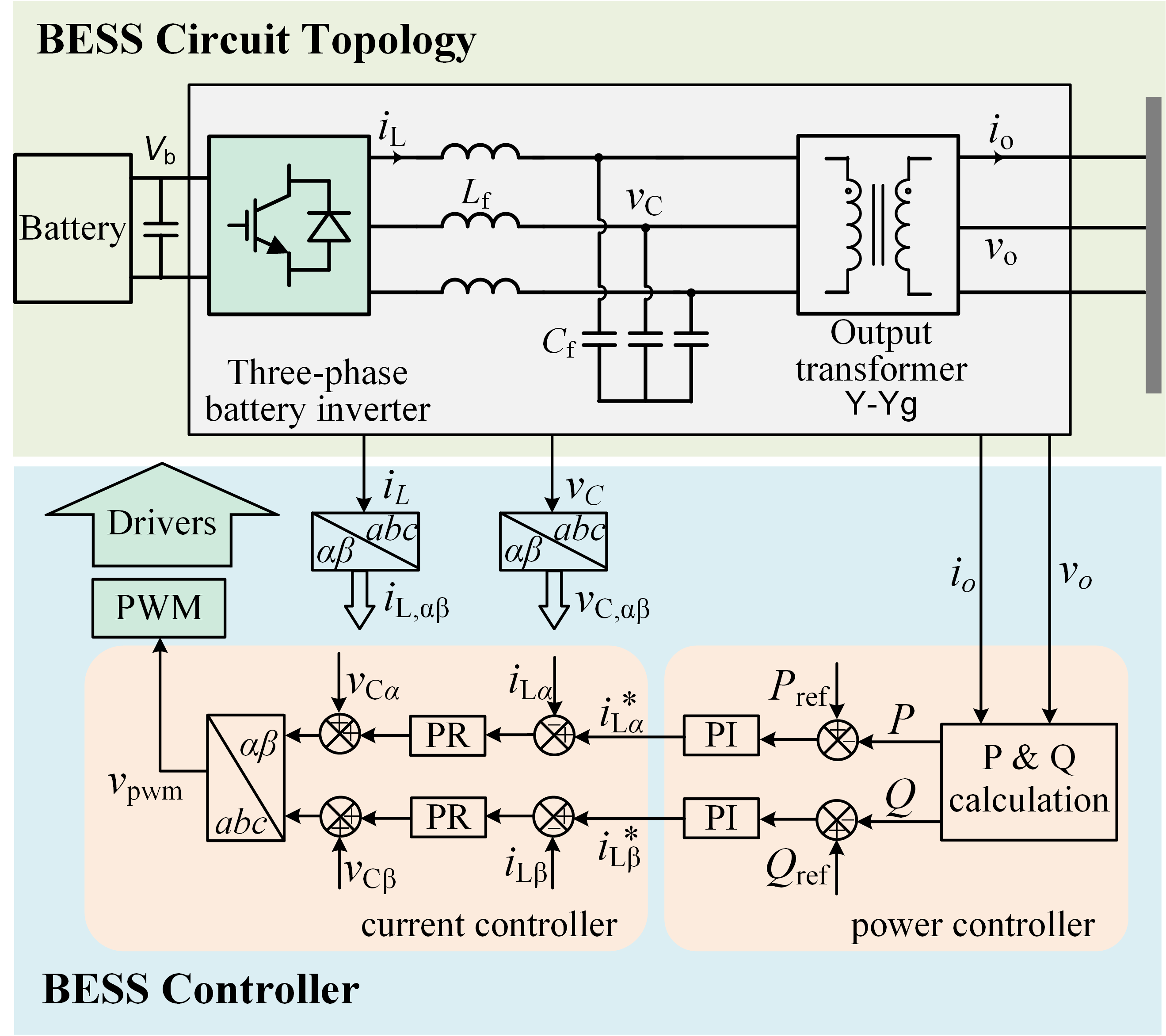
Figure 3: BESS circuit and control system diagram.

The control system is developed in the $\alpha\beta$ stationary reference frame (SRF), which requires one pair of PI controllers for power setpoint regulation, and one pair of proportional-resonant (PR) controllers for current regulation in the AC domain. The PR controllers transfer function is given by:

$$G_{c}=K_{p}+\frac{2K_{r}\omega_{c}s}{s^{2}+2\omega_{c}s+4\omega_{0}^{2}}$$ (6)

where $K_{r}$ is the resonant gain at 2$\omega$, $\omega_{c}$ is the cut-off frequency, and $\omega_{0}$ is the grid’s nominal frequency [16].

The modulation signal ($v_{\mathrm{pwm}}$) is generated by adding the output of the PR controllers with a feedforward signal of the output capacitor voltage. The authors present more details on the SRF control with an Y-Yg output transformer in [17]. The inverter is built with an averaged model of a two-level VSC developed in [18]. Efficiency factors ($\eta_{\mathrm{charge}}$, $\eta_{\mathrm{discharge}}$) are used to represent the battery charging and discharging modes, respectively.

II-C Lithium-Ion Battery Model

Figure 4 displays a second-order dynamic model of a lithium-ion battery that has been introduced in [19]. The model is built by a combination of current and voltage sources that are used to recreate the realistic behavior of a lithium-ion battery under output current steps. The battery SOC is given by

$$SOC(t)=SOC_{0}-\int_{0}^{t}\frac{I_{\mathrm{b}}}{K_{\mathrm{age}}Q_{\mathrm{c}}}\,dt$$ (7)

where $Q_{\mathrm{c}}$ is the battery rated capacity and $K_{\mathrm{age}}$ is an aging factor. In this paper, we consider real-time operation and set $K_{\mathrm{age}}=1$.

The model contains two RC parallel branches ($R_{\mathrm{ts}}$, $C_{\mathrm{ts}}$) and ($R_{\mathrm{tl}}$, $C_{\mathrm{tl}}$) to represent the short-term and long-term voltage drops due to current step responses, respectively. Furthermore, a series resistor $R_{\mathrm{s}}$ is modeled to represent an internal instantaneous voltage drop due to the battery current. The dynamic response of the battery’s internal voltages ($V_{\mathrm{Cts}}$, $V_{\mathrm{Ctl}}$) are given as follows.

$$\frac{dV_{\mathrm{Cts}}}{dt}=\frac{I_{\mathrm{b}}}{C_{\mathrm{ts}}}-\frac{V_{\mathrm{Cts}}}{R_{\mathrm{ts}}C_{\mathrm{ts}}}$$ (8)

$$\frac{dV_{\mathrm{Ctl}}}{dt}=\frac{I_{\mathrm{b}}}{C_{\mathrm{tl}}}-\frac{V_{\mathrm{Ctl}}}{R_{\mathrm{tl}}C_{\mathrm{tl}}}$$ (9)

The battery cell open-circuit voltage ($V_{\mathrm{oc}}$($V_{\mathrm{SOC}}$)) is a function of the instantaneous SOC value ($V_{\mathrm{SOC}}$). Experiments can be carried to obtain the relation between the battery internal voltage and its SOC. In [20], the relation is obtained via curve-fitting, and a seventh-order polynomial is built as follows:

$$V_{oc}(V_{SOC})=a_{1}{V_{SOC}}^{7}+a_{2}{V_{SOC}}^{6}+a_{3}{V_{SOC}}^{5}+a_{4}{V_{SOC}}^{4}+$$

$$a_{5}{V_{SOC}}^{3}+a_{6}{V_{SOC}}^{2}+a_{7}V_{SOC}+a_{8}$$ (10)

Hence, the battery output voltage ($V_{\mathrm{b}}$) is defined by

$$V_{\mathrm{b}}=V_{\mathrm{oc}}(V_{\mathrm{SOC}})-V_{\mathrm{Cts}}-V_{\mathrm{Ctl}}-R_{\mathrm{s}}I_{\mathrm{b}}$$ (11)

Figure 4: Second-order equivalent lithium-ion battery model.

It is important to mention that the RC parameters of the second-order lithium-ion battery model from [19] are approximately constant between 20% to 100% SOC operation, but they change exponentially between 0% to 20% SOC. Consequently, the modeling approach presented here is only valid if the SOC is maintained above 20% at all times. Moreover, a self-discharging resistor could be added in parallel to $Q_{\mathrm{c}}$ in Fig. 4 to represent the battery self-discharge of 2-10% per month, but this can be neglected for systems that are cycled often and/or do not leave the battery stored for a long time. Furthermore, as pointed in [19], in reality, all parameters from the second-order model are multivariable functions of SOC, current, temperature, and number of cycles. Nevertheless, the model can still present satisfactory performance for most application if a certain error tolerance is acceptable. Because the main focus of this work is not on developing an extremely accurate battery model, it is assumed the parameters are constant within the 20 to 100% SOC range.

II-D Hybrid PV Plant State-Space Model

The hybrid PV plant SS proposed in this work is designed with five state variables, which are assigned as: the battery SOC ($x_{1}$), the battery short-term internal voltage drop $V_{\mathrm{Cts}}$ ($x_{2}$), the battery long-term internal voltage drop $V_{\mathrm{Ctl}}$ ($x_{3}$), the battery current $I_{\mathrm{b}}$ ($x_{4}$), and the PV dc output power $P_{\mathrm{pv}}$ ($x_{5}$). Note the battery current and the PV output power are set as state variables so that constraints can be established for them in the MPC solver utilized in this work.

The hybrid PV plant has two main control inputs: change in battery output current ($u_{1}$) and change in PV dc output power ($u_{2}$). The control inputs are set as derivatives instead of the actual battery current and PV output power so that state variables can be assigned to the actual battery current and PV output power. Furthermore, the system also contains one input disturbance, corresponding to the maximum available PV dc power, $P_{\mathrm{mp}}$ ($u_{3}$). The disturbance is a measurable signal that comes from the MPPE algorithm presented in [4]. It is used to provide the MPC with constraints for the maximum PV power available. Inputs $u_{1}$ and $u_{2}$ are constrained within the ramp-up and ramp-down rate limits of the BESS and PV system by (12) and (13).

$$u_{1}=\frac{dI_{\mathrm{b}}}{dt},\quad-I_{\mathrm{b},\mathrm{rate}}\leq u_{1}\leq I_{\mathrm{b},\mathrm{rate}}$$ (12)

$$u_{2}=\frac{dP_{\mathrm{pv}}}{dt},\quad-P_{\mathrm{pv},\mathrm{rate}}\leq u_{2}\leq P_{\mathrm{pv},\mathrm{rate}}$$ (13)

$$u_{3}=P_{\mathrm{\mathrm{mp}}},\quad\text{from (\ref{eq:Pmp2})}$$ (14)

The model is designed with five output variables, which are assigned as: the hybrid plant output power ($y_{1}$), the battery current ($y_{2}$), the battery SOC ($y_{3}$), the power reserves ($y_{4}$), and the PV dc output power ($y_{5}$). The battery current, SOC, and the PV output power are defined as output variables to allow the implementation of soft constraints to the respective state variables when designing the MPC. Thus, the hybrid PV plant output power is given by (15), whereas the power reserves are given by (16).

$$y_{1}=P_{\mathrm{out}}=\eta_{\mathrm{bess}}\Big{[}V_{oc}(x_{1})-V_{\mathrm{ts}}-V_{\mathrm{tl}}-R_{\mathrm{s}}I_{\mathrm{b}}\Big{]}I_{\mathrm{b}}+\eta_{\mathrm{pv}}P_{\mathrm{pv}}$$ (15)

$$y_{4}=P_{\mathrm{res}}=\eta_{\mathrm{bess}}\Big{[}P_{\mathrm{bess}}^{N}-\big{(}V_{oc}(x_{1})-V_{\mathrm{ts}}-V_{\mathrm{tl}}-R_{\mathrm{s}}I_{\mathrm{b}}\big{)}I_{\mathrm{b}}\Big{]}+$$

$$\eta_{\mathrm{pv}}(P_{\mathrm{mp}}-P_{\mathrm{pv}})$$ (16)

In (16), $P_{\mathrm{bess}}^{N}$ is the battery nominal power. The PV and BESS unit efficiency factors ($\eta_{\mathrm{pv}}$, $\eta_{\mathrm{bess}}$) both include the inverter and output transformer losses. In addition, the BESS efficiency factor is based on the charging or discharging operation of the battery by (17).

$$\eta_{\mathrm{bess}}=\begin{cases}\eta_{\mathrm{discharge}}&\text{if $I_{\mathrm{b}}\geq 0$}\\ \eta_{\mathrm{charge}}&\text{if $I_{\mathrm{b}}<0$}\end{cases}$$ (17)

Thus, the SS of the system is defined as follows.

$$\dot{\mathbf{x}}=A\mathbf{x}+B\mathbf{u}$$

$$\mathbf{y}=C\mathbf{x}+D\mathbf{u}$$ (18)

$$\begin{bmatrix}\dot{x_{1}}\\[2.84544pt] \dot{x_{2}}\\[2.84544pt] \dot{x_{3}}\\[2.84544pt] \dot{x_{4}}\\[2.84544pt] \dot{x_{5}}\end{bmatrix}=\begin{bmatrix}0&0&0&\tfrac{\text{-}1}{Q_{\mathrm{c}}}&0\\[2.84544pt] 0&\tfrac{\text{-}1}{R_{\mathrm{ts}}C_{\mathrm{ts}}}&0&\tfrac{1}{C_{\mathrm{ts}}}&0\\[2.84544pt] 0&0&\tfrac{\text{-}1}{R_{\mathrm{tl}}C_{\mathrm{tl}}}&\tfrac{1}{C_{\mathrm{tl}}}&0\\[2.84544pt] 0&0&0&0&0\\[2.84544pt] 0&0&0&0&0\end{bmatrix}\begin{bmatrix}x_{1}\\[2.84544pt] x_{2}\\[2.84544pt] x_{3}\\[2.84544pt] x_{4}\\[2.84544pt] x_{5}\end{bmatrix}+\begin{bmatrix}0&0&0\\[2.84544pt] 0&0&0\\[2.84544pt] 0&0&0\\[2.84544pt] 1&0&0\\[2.84544pt] 0&1&0\\ \end{bmatrix}\begin{bmatrix}u_{1}\\ u_{2}\\ u_{3}\end{bmatrix}$$ (19)

$$\begin{bmatrix}y_{1}\\[2.84544pt] y_{2}\\[2.84544pt] y_{3}\\[2.84544pt] y_{4}\\[2.84544pt] y_{5}\end{bmatrix}=\begin{bmatrix}0&0&0&\eta_{\mathrm{bess}}\Big{[}V_{\mathrm{oc}}(x_{1})\textrm{-}x_{2}\textrm{-}x_{3}\textrm{-}R_{s}x_{4}\Big{]}&\eta_{\mathrm{pv}}\\[0.0pt] 0&0&0&1&0\\[0.0pt] 1&0&0&0&0\\[0.0pt] 0&0&0&\textrm{-}\eta_{\mathrm{bess}}\Big{[}V_{\mathrm{oc}}(x_{1})\textrm{-}x_{2}\textrm{-}x_{3}\textrm{-}R_{s}x_{4}\Big{]}&\textrm{-}\eta_{\mathrm{pv}}\\[0.0pt] 0&0&0&0&1\end{bmatrix}\begin{bmatrix}x_{1}\\[2.84544pt] x_{2}\\[2.84544pt] x_{3}\\[2.84544pt] x_{4}\\[2.84544pt] x_{5}\end{bmatrix}+$$

$$\begin{bmatrix}0&0&0&0&0\\[0.0pt] 0&0&0&0&0\\[0.0pt] 0&0&0&\eta_{\mathrm{pv}}&0\end{bmatrix}^{T}\begin{bmatrix}u_{1}\\ u_{2}\\ u_{3}\end{bmatrix}{\color[rgb]{1,1,1}+}\hskip 42.67912pt$$ (20)

The battery open-circuit voltage, $V_{\mathrm{oc}}(x_{1})$, is defined by (10). It is worth mentioning the initial condition of the power reserves is set as $\eta_{\mathrm{bess}}P_{\mathrm{bess}}^{N}$. Furthermore, note the controllability matrix of the proposed SS model, given by R = [B   AB   A²B   …   A^n-1B], presents full rank, confirming that all states of the system are controllable.

II-E Model Predictive Control Design

In this work, the optimal operation of the hybrid PV plant is achieved by the implementation of a MPC, which utilizes feedback control to solve for the optimal operation of the system while maintaining inputs and outputs within constraints that respect the physical limitations of the components. Figure 5 depicts the operation of a MPC. The prediction horizon, $p$, at time $k$, represents how many steps ahead the controller considers for the optimization, whereas the control horizon, $m$, at time $k$, corresponds to how many control steps are optimized within a given prediction horizon. Note that when the MPC is designed with $m<p$, the optimal inputs, $u_{k}$, are fixed at the last optimized value of the control horizon until the end of the prediction horizon, $p$.

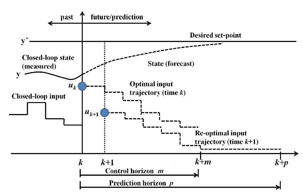
Figure 5: MPC prediction and control horizons. Modified from [21].

The objective of the optimal control problem is to find a sequence of optimal control signals, $z_{k}$, given in (21), to follow the targeted output signals, $y_{j}(i)$, $i\in p$.

$$z_{k}^{T}=\Big{[}u(k)^{T}\hskip 5.0ptu(k+1|k)^{T}\hskip 5.0pt...\hskip 5.0ptu(k+p-1|k)^{T}\Big{]},$$

$$\text{if }m<p\quad u(k+m+1:k+p-1|k)^{T}=u(k+m|k)^{T}$$ (21)

The MPC problem can be formulated as

$$\min J_{\epsilon}(z_{k})+J_{y}(z_{k})+J_{\Delta u}(z_{k})$$ (22)

$$J_{y}(z_{k})=\sum_{j=1}^{n_{y}}\sum_{i=1}^{p}\Bigg{\{}\frac{w_{j}^{y}}{s_{j}^{y}}\bigg{[}(y_{j}^{*}(k+i|k)-y_{j}(k+i|k)\bigg{]}\Bigg{\}}^{2}$$ (23)

$$J_{\Delta u}(z_{k})=\sum_{j=1}^{n_{u}}\sum_{i=0}^{p-1}\Bigg{\{}\frac{w_{j}^{\Delta u}}{s_{j}^{u}}\bigg{[}(u_{j}(k+i|k)-u_{j}(k+i-1|k)\bigg{]}\Bigg{\}}^{2}$$ (24)

where $J_{y}(z_{k})$ is the tracking error cost, $J_{\Delta u}(z_{k})$ is the cost associated with penalizing aggressive control moves, $J_{\epsilon}$ is a penalty factor associated with constraint violations, $w_{j}^{y}$ and $s_{j}^{y}$ are the cost weights and scale factors for the jth plant output ($y_{j}$), respectively, $k$ is the current control interval, $p$ is the size of the prediction horizon, $n_{y}$ is the number of plant output variables, $w_{j}^{\Delta u}$ and $s_{j}^{u}$ are the cost weights and scale factors for the jth control input ($u_{j}$), respectively, and $n_{u}$ is the number of plant control signals.

The constraint violation cost, $J_{\epsilon}(z_{k})$, ensures the solver can maintain numerical stability during real-time operation if the solution becomes unfeasible. Furthermore, to avoid numerical instabilities caused by hard constraints, the battery current, battery SOC, and the power reserves are set with soft constraints. More details on the penalty factor for handling constraint violations are presented in [22].

In (23), the tracking cost weights ($w_{j}^{y}$) must be tuned so the desired operation performance is achieved. For the hybrid PV plant, the main goal is to track an output power reference defined in (15), hence its weight is set with the highest value. Moreover, some of the weights will always be zero, such as the weights of the battery current ($w_{2}^{y}$) and the PV output power ($w_{5}^{y}$), because there is no specific goal for each of them individually.

In (24), the penalization of aggressive control moves incentives the controller to maintain a smooth operation when trying to optimize the tracking error cost, and helps maintaining good numerical conditioning.

The weight of the battery SOC ($w_{3}^{y}$) is set to a small value with a high setpoint (e.g., 90%). With those settings, the MPC will boost the battery SOC to higher levels when possible, but it will significantly prioritize the power setpoint tracking during operation. It is worth mentioning that leaving a lithium-ion battery to linger at a fully charged state will accelerate their aging process [23]; therefore, it may be preferred to not set the BESS SOC setpoint to 100%.

Due to the nonlinear characteristics of the hybrid PV plant SS model, traditional linear MPC design is not appropriate. The MPC Toolbox from [22] is compatible with the eMEGASIM environment from OPAL-RT utilized for real-time simulations and provides multiple options for the implementation of MPCs that can handle nonlinear models, such as: (a) Adaptive MPC, (b) Gain-Scheduled MPC, and (c) Nonlinear MPC. In this work, best performance was found with the adaptive MPC. Figure 6 displays the proposed control strategy. The adaptive MPC sends the power setpoints to the plant comprised of the PV and BESS unit. Sensors measure the PV output power as well as the battery voltage and current, which are inserted in an EKF that estimates the system states. PV forecasts and information about the instantaneous maximum available PV power are also inputs of the adaptive MPC. In the figure, the hybrid PV plant setpoints are generated by an external energy management system (EMS) running in an external controller.

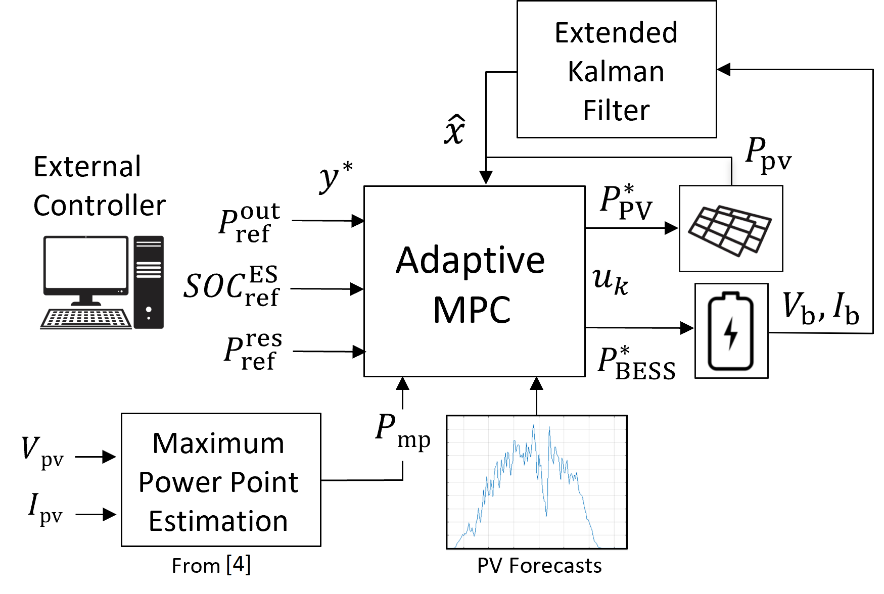
Figure 6: Configuration of the model predictive controller.

Three main parameters must be defined when designing the MPC: timestep ($T_{\mathrm{mpc}}$), prediction horizon, and the control horizon. In this work, the timestep is set as 3 seconds, whereas the prediction horizon is selected as 400 steps (20 minutes), which is long enough to account for the battery slow charging/discharging dynamics. Note the timestep could be reduced to 2 or even 1 second(s) if real-time operation can be maintained by the real-time simulator, but it should not be increased further, as this will deteriorate the MPC’s response to irradiance transients. The control horizon is set to 20 steps, based on the length of the ultra short-term PV forecasting. The estimated PV power ($P_{\mathrm{mp}}$) is used both as a disturbance applied to the power reserves and as an upper constraint to the PV output power.

By actuating as a time-varying upper constraint being updated in real time, $P_{\mathrm{mp}}$ forces the MPC to consider what is the actual available PV power when solving for the optimal control commands. It is worth mentioning that time-varying upper bounds capable of being updated in real time is a feature from the MPC Toolbox [24] that only became compatible with RT-LAB version 2021.2, which is the platform used to run eMEGASIM models in real-time simulations.

II-F PV Forecast

We consider the employment of two forecast techniques to the hybrid PV plant: (i) an ultra-short-term forecast of the available PV power with skycams [25], and a 20 minutes ahead forecast of the average available PV power.

It is assumed the 20-minutes ahead forecast performs with $\pm$10% errors. For the ultra-short-term forecast, it is assumed that the PV plant runs the algorithm proposed in [26], which has been experimentally validated with 70 inverters of a 48 MWdc plant. The method reported a relative root mean square error (rRMSE) of 3.2% for its 20-seconds ahead forecast, and an approximately linear error increase up to 8.2% at its 60-seconds ahead forecast. Therefore, we utilize the ultra-short-term forecasting only for the first 60 seconds, which is also defined as the length of the control horizon of the adaptive MPC.

Figure 7: Illustration of how the nowcasting performance is replicated.

Figure 7 demonstrates how the performance of the ultra-short-term forecasting method is simulated for a system with an MPC step of 3 seconds and a control horizon of 60 seconds. First, a normal distribution is sampled every few minutes to generate an artificial performance error. Next, the new error value is filtered by a low-pass filter with a time constant of one minute. The filter ensures the estimations will not be instantaneously stepped up or down as new error values are sampled, providing a more realistic transition between different estimation errors. Then, the filtered error factor ($e$) is applied to the actual $P_{\mathrm{mp}}$ values, which are constantly being stored and updated in an auxiliary vector. By reducing the error factor ($e$) from its full value at the 60-seconds ahead forecast down to $0.05e$ at the 3-seconds ahead forecast, the estimation accuracy is linearly improved as the prediction length is reduced.

II-G Battery State Estimation

In practice, the battery states cannot be directly measured. Thus, in this paper, we use an EKF (see Fig. 6) to estimate the battery states ($\hat{x}$) using battery voltage and current measurements as inputs. Gaussian noises are added to the measurements to match the signal-to-noise (SNR) ratios expected from standard dc sensors. Because the EKF theory is well established in the literature, it will not be discussed here.

III Real-Time Simulation Results

To validate the proposed algorithm, a testbed is set up on an OPAL-RT real-time simulator. As shown in Fig. 8, the hybrid PV plant consists of four equal 612 kWdc PV arrays, a plant controller, and a 1.2 MVA grid-following BESS. The BESS has a 1 MW/0.25 MWhdc lithium-ion battery unit and assists with the intra-minute power management. Table I lists the simulation parameters. For more details on the MPC implementation, PV forecasting representation, and simulation settings, please refer to [27].

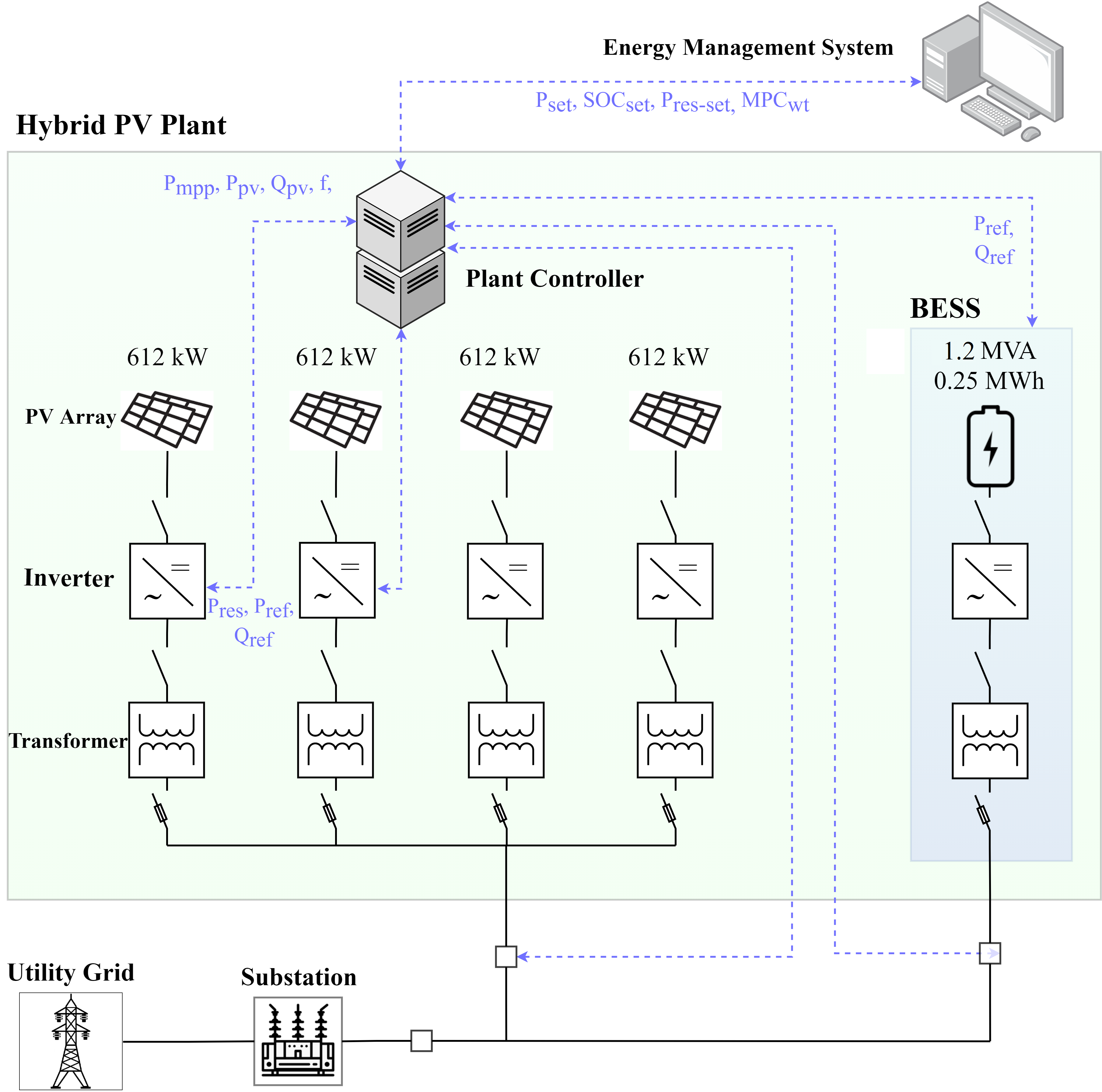
Figure 8: Configuration of the hybrid PV plant.

The high-resolution (one-second) irradiance and temperature data used to set up the simulation are collected by Strata Solar at a 5.04 MW solar farm located in North Carolina, USA, on April 8^th (Fig. 9) and 9^th (Fig. 10), 2022.

TABLE I: Hybrid PV Plant Model Parameters

	Power	4$\times$$612\text{\,}\mathrm{kW}$
	Module	CS6P-250P
	Size (parallel$\times$series)	153 $\times$ 16
PV Arrays	Vmp, Imp	$481.6\text{\,}\mathrm{V}$, $1270\text{\,}\mathrm{A}$
	Power, Frequency	$500\text{\,}\mathrm{k}\mathrm{V}\mathrm{A}$, $60\text{\,}\mathrm{Hz}$
	Voltage (line-line)	200 V (RMS)
	$\eta_{\mathrm{pv}}$	96.5%
	Ramp Rate	0.2 p.u./s
	Lf, rL	$100\text{\,}\mathrm{\SIUnitSymbolMicro H}$, $3\text{\,}\mathrm{m\SIUnitSymbolOhm}$
	Cdc	$5000\text{\,}\mathrm{\SIUnitSymbolMicro F}$
	PI (vdc)	Kp = 1, Ki = 250
PV Inverter	PI (id, iq)	Kp = 0.7, Ki = 50
	Power, Frequency	1.2 MVA, $60\text{\,}\mathrm{Hz}$
	Voltage (line-line)	480 V (RMS)
	Ramp Rate	0.2 p.u./s
	$C_{f}$, $L_{f}$	2 mF, $100\text{\,}\mathrm{\SIUnitSymbolMicro H}$
	PR controller	K${}_{\mathrm{p}}=2$, K${}_{\mathrm{r}}=100$
	$\eta_{\mathrm{charge}}$ (dc/ac)	96.5%
BESS	$\eta_{\mathrm{discharge}}$ (ac/dc)	96.5%
	Power, Capacity	1 MW / 0.25 MWh
	Voltage	1600 V
	Cells (series$\times$parallel)	441$\times$9
	$C_{\mathrm{ts}}$, $R_{\mathrm{ts}}$ (per cell)	440.57 F, 2 m$\Omega$
	$C_{\mathrm{tl}}$, $R_{\mathrm{tl}}$ (per cell)	17111 F, 4.2 m$\Omega$
	$R_{\mathrm{s}}$ (per cell)	1.3 m$\Omega$
Battery	$Q_{\mathrm{c}}$ (represents Ah)	160 F

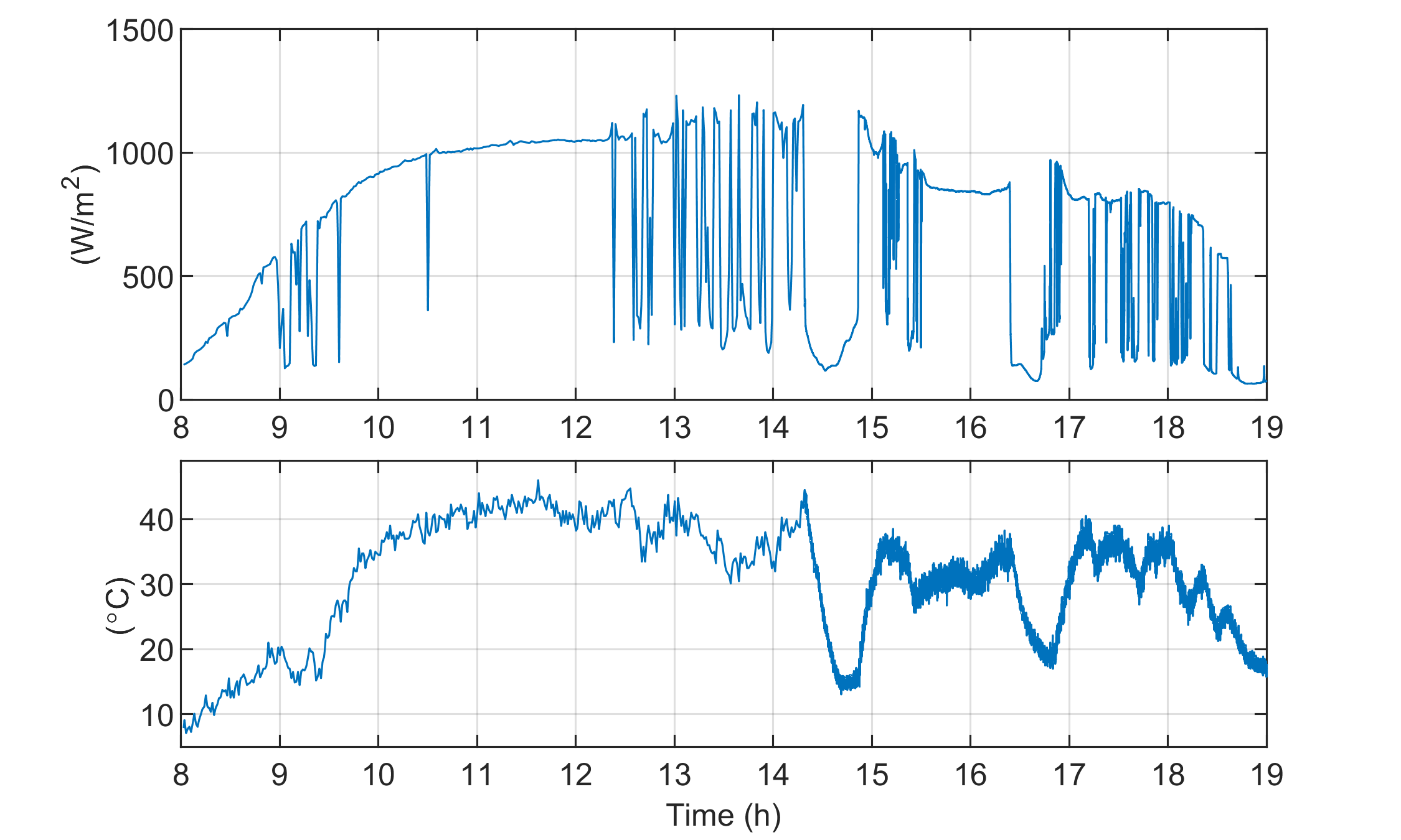
Figure 9: Irradiance and temperature data from day 1.

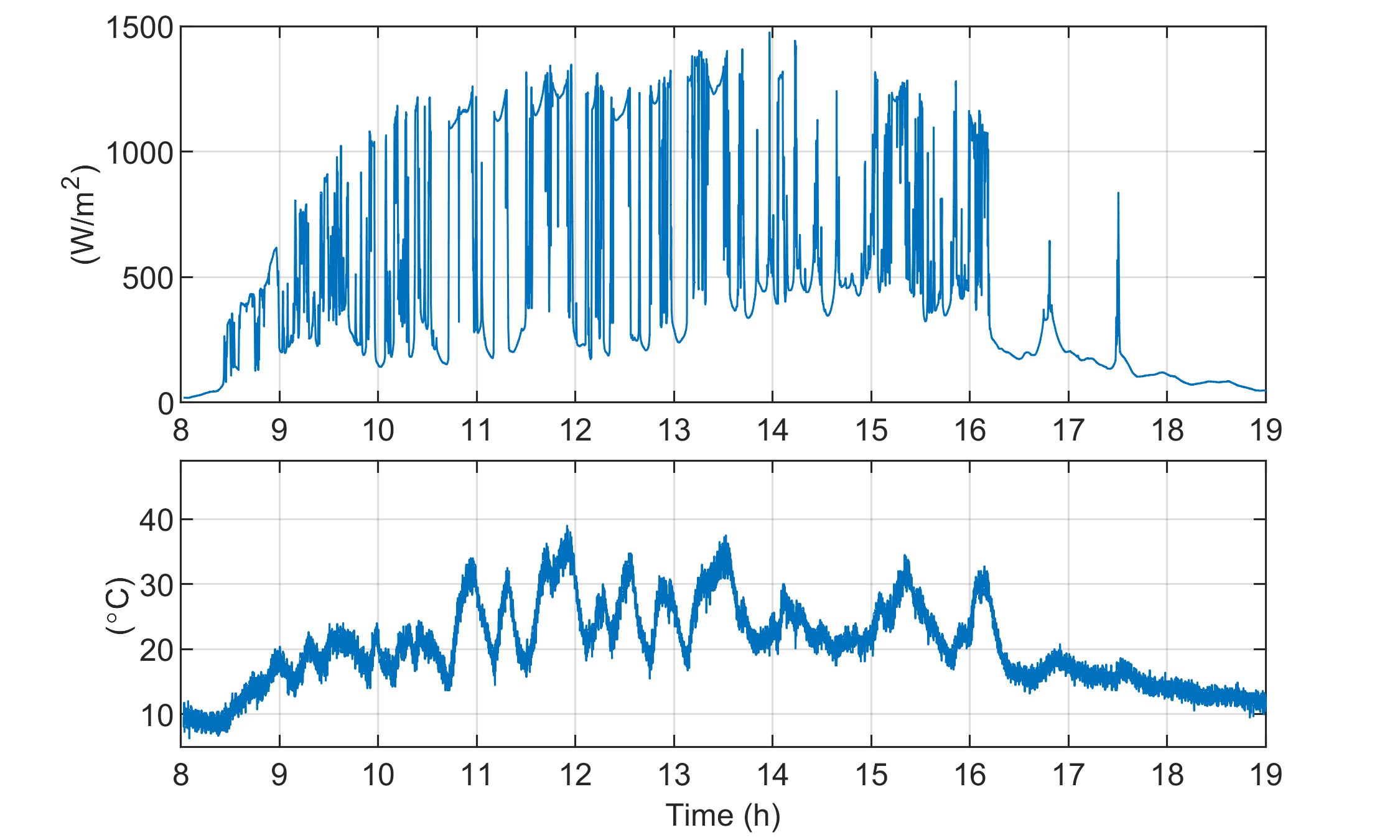
Figure 10: Irradiance and temperature data from day 2.

III-A Extended Kalman Filter Performance

In this section, we conduct an error sensitivity analysis for the EKF-based SOC estimation to demonstrate its limitations. This is done by adding errors to the parameters of the battery mathematical model given by (19) to represent cases where the battery parameters cannot be accurately estimated. Three scenarios are studied: (i) all battery parameters, i.e. ($R_{\mathrm{s}}$, $R_{\mathrm{ts}}$, $R_{\mathrm{tl}}$, $Q_{\mathrm{c}}$, $C_{\mathrm{ts}}$, and $C_{\mathrm{tl}}$) are modeled with +5% errors, (ii) all battery parameters are modeled with -5% errors, and (iii) the base case where battery parameters are known. Results are displayed in Fig. 11.

The RMSE errors in case (iii) are bounded by cases (i) and (ii). In (i), the SOC estimation was mostly above the actual SOC during discharging modes, and below the actual SOC during charging modes. The opposite was found for case (ii). In reality, a perfect extraction of the battery parameters is never possible because the battery parameters vary with respect to temperature, aging, etc. Therefore, the EKF estimation will be within an error margin. Consequently, in this paper, we set up a BESS SOC operation range to avoid overcharging.

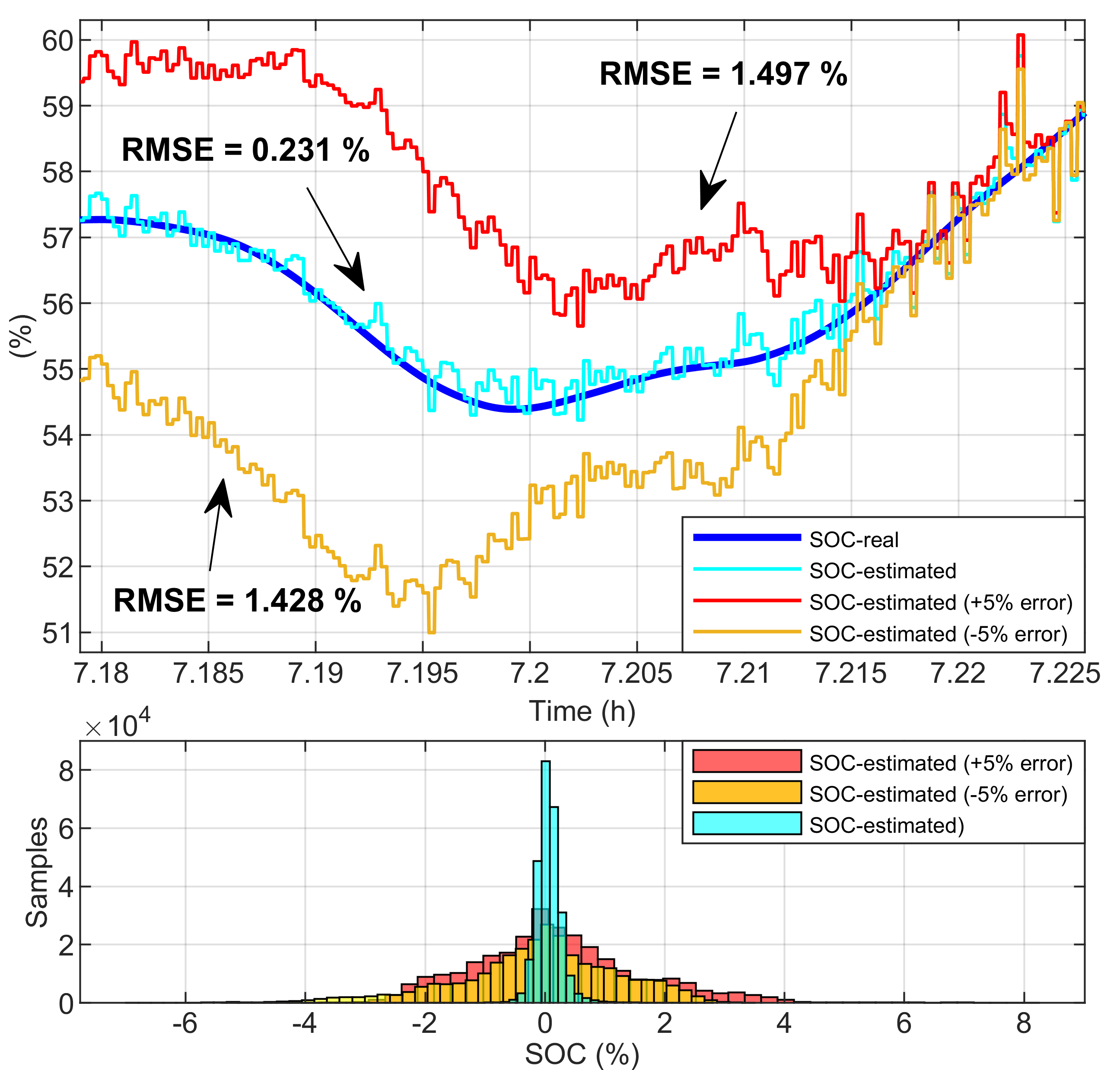
Figure 11: Performance of the EKF SOC estimation considering parameter errors.

Figure 12: Hybrid PV Plant performance in day 1 (case 1): (a) hybrid PV plant output power, (b) PV output power, (c) BESS output power, (d) battery SOC, and (e) power output errors, (f) power reserves.

III-B Power Regulation Performance

This section analyzes the capability of the hybrid PV plant to follow power setpoints while operating under high irradiance intermittency conditions. To provide regulation services, the power setpoint of the hybrid PV plant is determined in two steps. First, the forecasted 30-minute average output power of the PV plant (assuming the forecasting error is within $\pm$10%) is used to define the baseline power output of the plant for every 30-minute operation interval. Then, during each 30-minute interval, a 2-seconds 1 MW PJM regulation D signal (0.5 MW up/down with zero mean) is superimposed onto the 30-minute baseline to obtain the 2-second power setpoint.

In this case, the plant’s power reserves setpoint ($P_{\mathrm{ref}}^{\mathrm{reserves}}$) starts as 500 kW, and is reduced down to 0 as the regulation signal ranges from 0 to positive 500 kW. This means that when providing upward regulation (power injection increase), the power reserves constraint is alleviated based on the power request increase. Alternatively, the plant could have been set to provide only downward regulation while continuously maintaining power reserves for FFR.

Results of day 1 (case 1) are presented in Fig. 12. In this case, there are three main reasons for power output errors: (A) BESS SOC depletion, (B) power balance limitations due to extreme cloud coverage, and (C) power reserves constraints, which can be observed in Fig. 12(f) when the actual power reserves (in black) becomes smaller than the minimum power reserves requested (in red). Each cause of error is respectively labeled in Fig. 12(e).

Reason (C) can happen if high clouding events coincide with moments of high power setpoint request. When this happens, if the hybrid PV plant is asked to maintain power reserves, the problem becomes infeasible because either the power setpoint or the power reserves have to be violated. The trade-off between these two can be adjusted by increasing the softness of the power reserves constraint, where the operator can prioritize tracking power output setpoints or maintaining minimum power reserves for FFR services.

Errors originated from battery SOC depletion can be observed in Fig. 12(e) around hours 9.75, 14.75, and 16.6, whereas errors due to the hybrid PV plant reaching its output power limits can be seen at hours 9.6, 12.6, and 17.25. At hour 17.25, for example, the PV availability drops below 500 kW. This is because although the battery operates at the nominal output power (1 MW), the power setpoint of 2 MW cannot be maintained, causing a large output error. Errors due to power reserves reaching their limits can be seen around hours 9.3, 14.4 and 16.4 (see Fig. 12(f)).

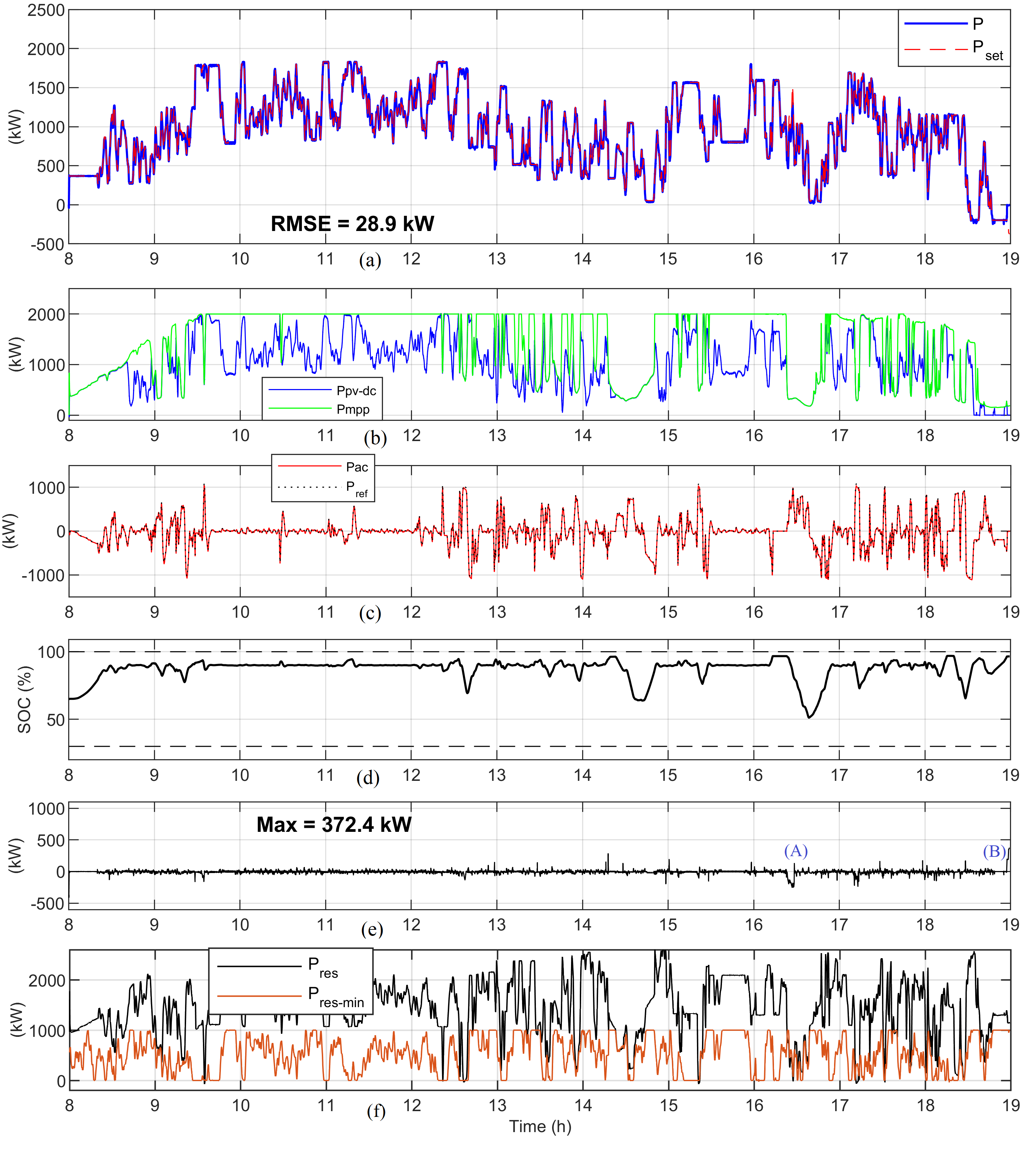
Figure 13: Hybrid PV Plant performance in day 1 (case 2): (a) hybrid PV plant output power, (b) PV output power, (c) BESS output power, (d) battery SOC, and (e) power output errors, (f) power reserves.

One solution to reduce the power setpoint error is to reduce the average output power requested such that the expected power from the plant assumes a more conservative approach. Thus, in Case 2, we reduce the average requested power by 25%. As shown in Fig. 13, the plant can provide a much closer power setpoint tracking if a less aggressive request is demanded from it. In this case, the plant power output RMSE reduced from 103.3 to 28.9 kW, close to four times smaller. Furthermore, by comparing Fig. 12(f) with 13(f), it can be noticed how in the second case the system is able to maintain higher power reserves. In this case, there are two main sources of errors: (A) power reserves limitations, and (B) BESS reaching upper SOC limits. Note the BESS upper SOC is limited to a value below 100% for two reasons: (i) providing a safety margin to accommodate for SOC estimation errors, and (ii) maintaining enough headroom for providing FFR services at anytime.

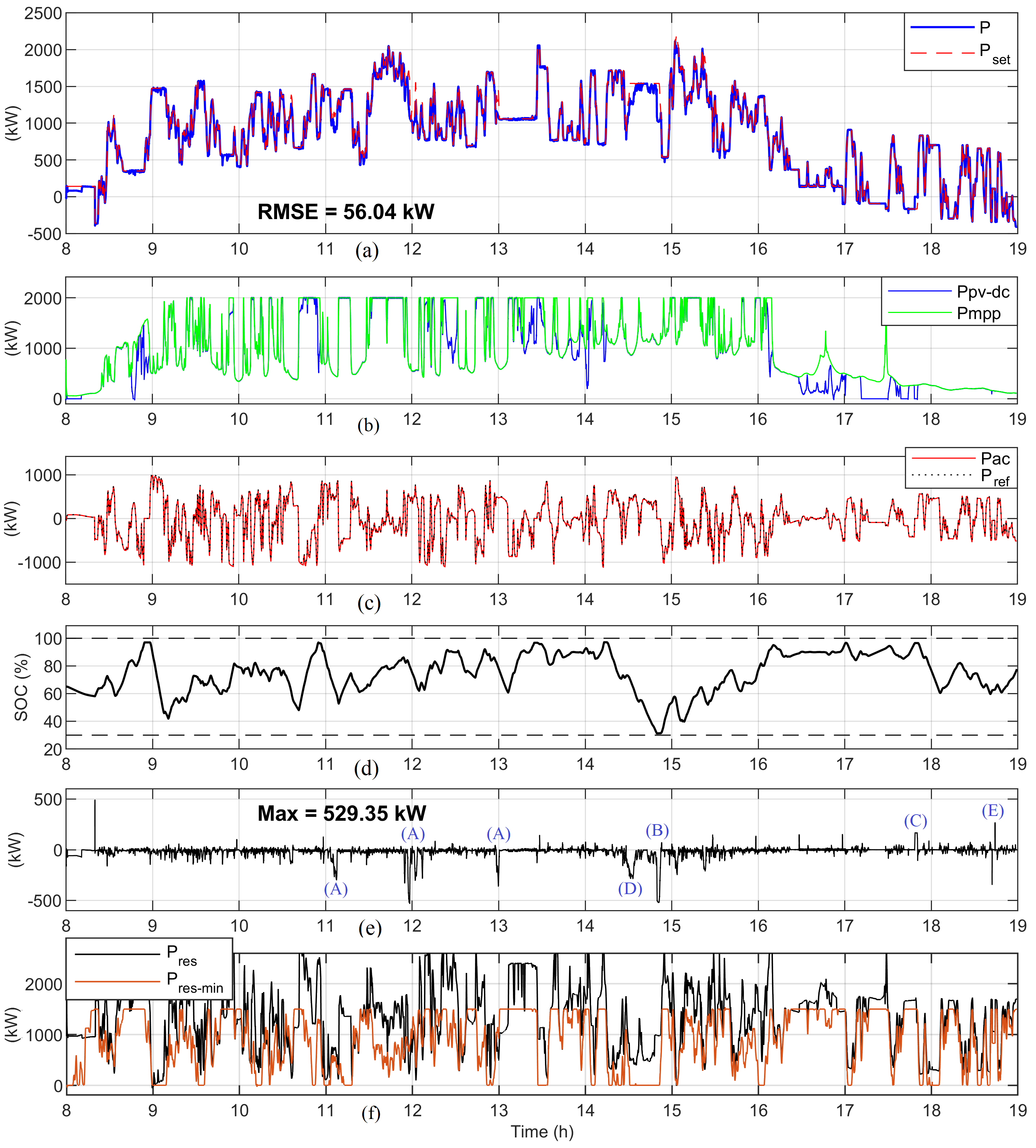
Figure 14: Hybrid PV Plant performance in day 2: (a) hybrid PV plant output power, (b) PV output power, (c) BESS output power, (d) battery SOC, and (e) power output errors, (f) power reserves, (f) power reserves.

Figure 14 displays the performance for the second day, corresponding to an extreme scenario of very high irradiance intermittency. Note there is a spike in the power output error around hour 8.3. This is because the regulation signal is activated at hour 8.3 (after 20 minutes). Thus, if a very high regulation value is received right upon activation (see Fig. 14(f), a large instantaneous error will occur because the plant must ramp up to its new setpoint.

In this case, the causes of errors are: (A) power reserves limits, (B) BESS SOC depletion, (C) BESS reaching upper SOC limits, (D) SOC usage optimization, (E) ramping limits. Note the error at hour 14.5 occurs even though the battery could have increased its power output. This is because after considering (i) the available PV (and its forecast), (ii) the requested power output, and (iii) the BESS increased losses at higher power outputs, the MPC optimization starts to degrade its power tracking performance to optimize the usage of available BESS SOC. On the other hand, during hours 11.1, 12, and 13, there are errors even though there is sufficient battery SOC, and the battery is not reaching its nominal ratings. Those errors occur because the system reaches its minimum power reserves constraint, and thus constraints’ violation weights are considered to decide how much of the power output should be sacrificed in exchange for reserve violations. This relation can be tuned as needed by adjusting the minimum and maximum output variables ECR gains ($y_{i,\mathrm{ECR}}^{\mathrm{min}}$, $y_{i,\mathrm{ECR}}^{\mathrm{max}}$), given in the Appendix section.

In addition, a positive error is observed around hour 17.8. It occurred because the battery reached its upper SOC limit, so the hybrid PV plant was incapable of absorbing power for a downward regulation.

III-C Comparison to a Thermal Machine

Next, the power regulation of the hybrid PV plant is compared to that of a typical PJM thermal unit with a ramping of 0.8 MW per minute [28] during day 2. The machine model is built with governor, turbine, and reheater time constants given in [29]. The hybrid plant SOC setpoint is dropped from 90% to 80% to leave more room for downward regulation, and the average power requested is reduced by 20%. The same power setpoint is requested from both systems, with a power regulation signal of 1.5 MW. Because the thermal unit cannot absorb power, its power setpoint is offset by 750 kW for the entire operation.

As shown in Figs. 15 and 16, compared to the hybrid PV plant, the thermal machine has a slower response rate and consequently, a significant higher power output error. In Fig. 15(c), we highlight five factors causing power output error in the hybrid PV plant operation: (A) hitting battery upper SOC limit, (B) hitting battery lower SOC limit, (C) reaching power reserves limits, (D) limited by the SOC usage optimization requirement, and (E) hitting ramping constraints.

Figure 17 presents an analysis of the errors in power output and power reserves requested through the presented cases. As can be seen in Figs. 17(a) and 17(b), when reducing the average power output request by 25% from case 1, the performance tracking performance can be significantly improved, with power reserves being successfully maintained throughout 96.65% of the operation time. This demonstrates that an oversized hybrid PV plant can become a reliable source of power reserves even if the plant follows variable power setpoints in days of high irradiance intermittency.

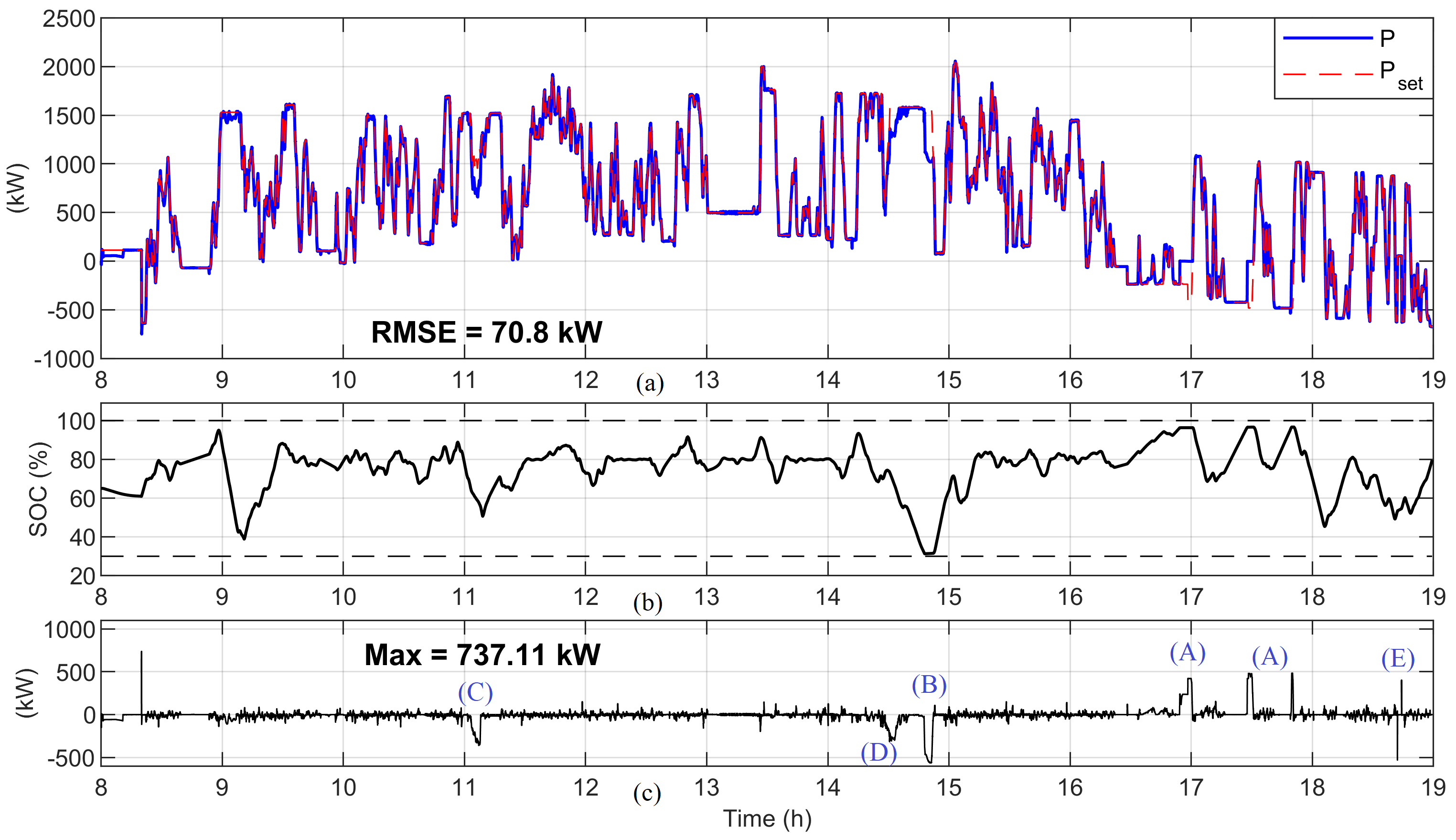
Figure 15: Hybrid PV Plant performance in day 2 (providing 1.5 MW regulation service): (a) power output, (b) battery SOC, (c) power output error.

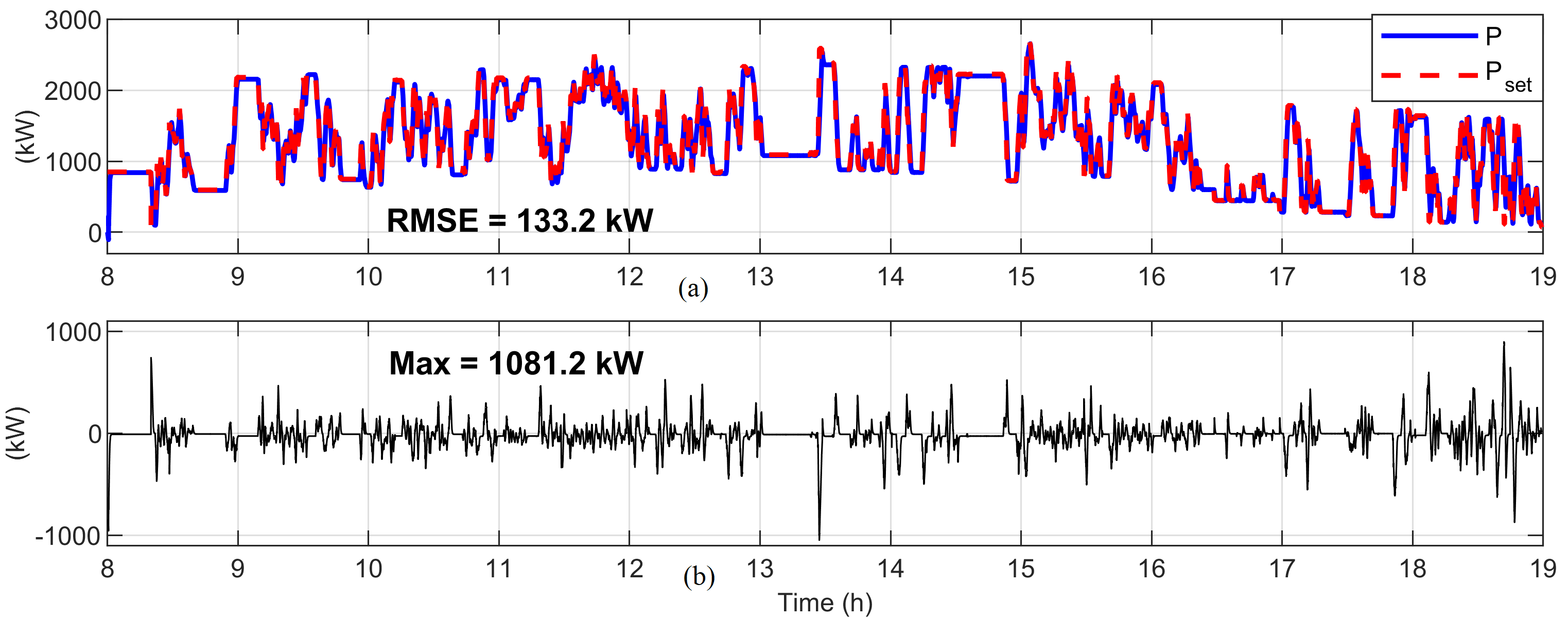
Figure 16: Thermal generator performance following same power setpoint in day 2 (providing 1.5 MW regulation service): (a) power output, (b) power output error.

Figure 17(c) compares the power output error between the Hybrid PV plant and the thermal unit. The results show the hybrid PV plant can provide superior regulation performance due to its faster IBR controls. Note that the thermal unit has a typical ramping of 0.8 MW per minute. In this test, we set the hybrid PVplant ramping at 0.6 MW per second, although in practice, the PV plant ramping could be even faster based on the agreement with the system operator. Moreover, it is important to highlight that day 2 is a day of very high intermittency (Fig. 10), selected to demonstrate performance limitations for the worst case scenario.

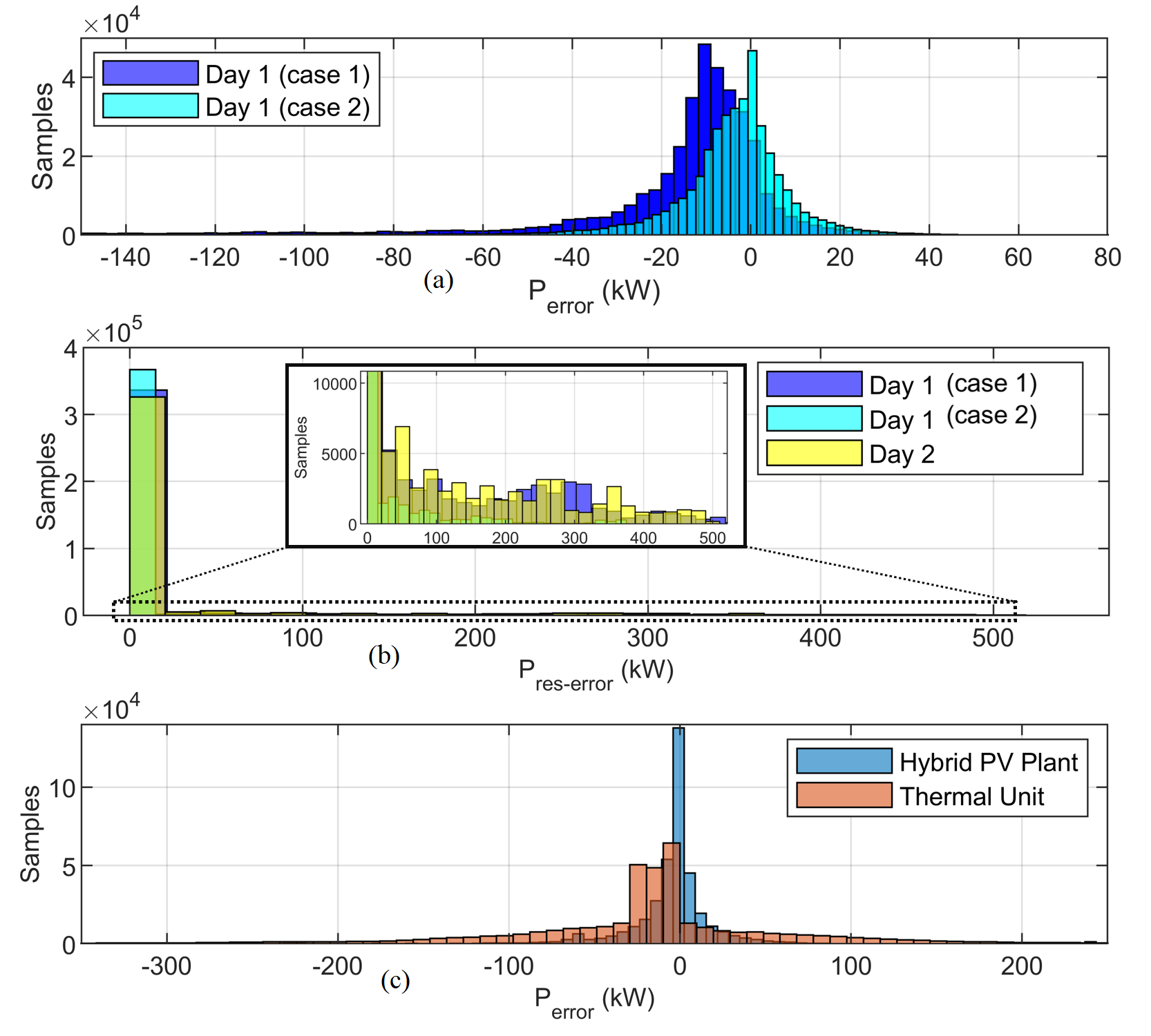
Figure 17: Comparison of setpoint tracking errors: (a) power output of day 1 (cases 1 and 2), (b) power reserves of day 1 (cases 1 and 2) and day 2, (c) power output between hybrid PV plant and thermal unit in day 2.

IV Conclusion

This work proposes a control strategy to optimally operate a hybrid PV plant while considering power reserves for providing FFR services. The system combines optimal control with the power curtailment algorithm introduced in [4] to form a PV plant capable of maintaing reserves for providing both regulation and/or FFR services for grid support. An adaptive MPC is utilized to handle the nonlinearities of the plant model, and detailed EMT models are developed to provide an accurate representation of components losses and limitations. Results demonstrate the system can provide high quality power regulation services as well as maintain robust power reserves without the need for large BESS storage. Furthermore, the proposed framework is highly customizable, such that constraint softness and adjustable control objective weights can be used to shift priorities between power regulation, power reserves, or battery SOC management in real-time.

References

- [1] H. Yuan, J. Tan, Y. Zhang, S. Murthy, S. You, H. Li, Y. Su, and Y. Liu, “Machine learning-based PV reserve determination strategy for frequency control on the WECC system,” in 2020 IEEE Power & Energy Society Innovative Smart Grid Technologies Conference (ISGT). IEEE, 2020, pp. 1–5.
- [2] I. S. Association et al., “IEEE Std. 1547-2018,” Standard for Interconnection and Interoperability of Distributed Energy Resources with Associated Electric Power Systems Interfaces, 2018.
- [3] California Public Utilities Commission et al., “Electric rule no. 21 generating facility interconnections,” 2016.
- [4] V. D. Paduani, H. Yu, B. Xu, and N. Lu, “A unified power-setpoint tracking algorithm for utility-scale PV systems with power reserves and fast frequency response capabilities,” IEEE Transactions on Sustainable Energy, vol. 13, no. 1, pp. 479–490, 2021.
- [5] J. Chang, Y. Du, E. G. Lim, H. Wen, X. Li, and L. Jiang, “Coordinated frequency regulation using solar forecasting based virtual inertia control for islanded microgrids,” IEEE Transactions on Sustainable Energy, vol. 12, no. 4, pp. 2393–2403, 2021.
- [6] V. Gevorgian, R. Wallen, P. Koralewicz, E. Mendiola, S. Shah, and M. Morjaria, “Provision of grid services by PV plants with integrated battery energy storage system,” National Renewable Energy Lab.(NREL), Golden, CO (United States), Tech. Rep., 2020.
- [7] S. Teleke, M. E. Baran, A. Q. Huang, S. Bhattacharya, and L. Anderson, “Control strategies for battery energy storage for wind farm dispatching,” IEEE Transactions on Energy Conversion, vol. 24, no. 3, pp. 725–732, 2009.
- [8] M. Z. Daud, A. Mohamed, and M. Hannan, “An improved control method of battery energy storage system for hourly dispatch of photovoltaic power sources,” Energy Conversion and Management, vol. 73, pp. 256–270, 2013.
- [9] S. Teleke, M. E. Baran, S. Bhattacharya, and A. Q. Huang, “Optimal control of battery energy storage for wind farm dispatching,” IEEE Transactions on Energy Conversion, vol. 25, no. 3, pp. 787–794, 2010.
- [10] A. Alaniz, “Model predictive control with application to real-time hardware and guided parafoil,” Ph.D. dissertation, Massachusetts Institute of Technology, 2004.
- [11] U. R. Nair, M. Sandelic, A. Sangwongwanich, T. Dragičević, R. Costa-Castelló, and F. Blaabjerg, “An analysis of multi objective energy scheduling in pv-bess system under prediction uncertainty,” IEEE Transactions on Energy Conversion, vol. 36, no. 3, pp. 2276–2286, 2021.
- [12] M. Lei, Z. Yang, Y. Wang, H. Xu, L. Meng, J. C. Vasquez, and J. M. Guerrero, “An mpc-based ess control method for PV power smoothing applications,” IEEE Transactions on Power Electronics, vol. 33, no. 3, pp. 2136–2144, 2017.
- [13] X. Li, D. Hui, and X. Lai, “Battery energy storage station (bess)-based smoothing control of photovoltaic (PV) and wind power generation fluctuations,” IEEE Transactions on Sustainable Energy, vol. 4, no. 2, pp. 464–473, 2013.
- [14] V. Paduani, L. Song, B. Xu, and N. Lu, “Maximum power reference tracking algorithm for power curtailment of photovoltaic systems,” in 2021 IEEE Power & Energy Society General Meeting (PESGM). IEEE, 2021, pp. 01–05.
- [15] V. Paduani and N. Lu, “Implementation of a two-stage PV system testbed with power reserves for grid-support applications,” in 2021 North American Power Symposium (NAPS). IEEE, 2021, pp. 1–6.
- [16] H. Cha, T.-K. Vu, and J.-E. Kim, “Design and control of proportional-resonant controller based photovoltaic power conditioning system,” in 2009 IEEE Energy Conversion Congress and Exposition. IEEE, 2009, pp. 2198–2205.
- [17] B. Xu, V. Paduani, D. Lubkeman, and N. Lu, “A novel grid-forming voltage control strategy for supplying unbalanced microgrid loads using inverter-based resources,” arXiv preprint arXiv:2111.09464, 2021.
- [18] A. Yazdani and R. Iravani, Voltage-Sourced Converters in Power Systems: modeling, control, and applications. John Wiley & Sons, 2010.
- [19] M. Chen and G. A. Rincon-Mora, “Accurate electrical battery model capable of predicting runtime and iv performance,” IEEE Transactions on Energy Conversion, vol. 21, no. 2, pp. 504–511, 2006.
- [20] Z. Chen, Y. Fu, and C. C. Mi, “State of charge estimation of lithium-ion batteries in electric drive vehicles using extended kalman filtering,” IEEE Transactions on Vehicular Technology, vol. 62, no. 3, pp. 1020–1030, 2012.
- [21] L. Dai, Y. Xia, M. Fu, and M. Mahmoud, “Discrete-time model predictive control,” Advances in Discrete Time Systems, pp. 77–116, 2012.
- [22] A. Bemporad, M. Morari, and N. L. Ricker, “Model predictive control toolbox user’s guide,” The Mathworks, 2010.
- [23] J. Vetter, P. Novák, M. R. Wagner, C. Veit, K.-C. Möller, J. Besenhard, M. Winter, M. Wohlfahrt-Mehrens, C. Vogler, and A. Hammouche, “Ageing mechanisms in lithium-ion batteries,” Journal of Power Sources, vol. 147, no. 1-2, pp. 269–281, 2005.
- [24] MATLAB, “Model predictive control toolbox release notes,” https://www.mathworks.com/help/mpc/release-notes.html, MATLAB. Retrieved: March 10, 2022.
- [25] T. Schmidt, M. Calais, E. Roy, A. Burton, D. Heinemann, T. Kilper, and C. Carter, “Short-term solar forecasting based on sky images to enable higher PV generation in remote electricity networks,” Renewable Energy and Environmental Sustainability, vol. 2, p. 23, 2017.
- [26] M. Lipperheide, J. Bosch, and J. Kleissl, “Embedded nowcasting method using cloud speed persistence for a photovoltaic power plant,” Solar Energy, vol. 112, pp. 232–238, 2015.
- [27] V. Daldegan Paduani, “Real-time modeling and control of ders with advanced grid-support functionalities.” Ph.D. dissertation, North Carolina State University, 2022.
- [28] B. Kirby and M. Milligan, “Method and case study for estimating the ramping capability of a control area or balancing authority and implications for moderate or high wind penetration,” National Renewable Energy Lab., Golden, CO (US), Tech. Rep., 2005.
- [29] S. Abd-Elazim and E. Ali, “Firefly algorithm-based load frequency controller design of a two area system composing of PV grid and thermal generator,” Electrical Engineering, vol. 100, no. 2, pp. 1253–1262, 2018.