Models of Rotating Infall for the B335 Protostar

Abstract

Models of the protostellar source, B335, are developed using axisymmetric three-dimensional models to resolve conflicts found in one-dimensional models. The models are constrained by a large number of observations, including ALMA, Herschel, and Spitzer data. Observations of the protostellar source B335 with ALMA show red-shifted absorption against a central continuum source indicative of infall in the HCO⁺ and HCN $J=4\rightarrow 3$ transitions. The data are combined with a new estimate of the distance to provide strong constraints to three-dimensional models including a rotating, infalling envelope, outflow cavities, and a very small disk. The models favor ages since the initiation of collapse between 3${}\times 10^{4}$ and 4${}\times 10^{4}$ yr for both the continuum and the lines, resolving a conflict found in one-dimensional models. The models under-predict the continuum emission seen by ALMA, suggesting an additional component such as a pseudo-disk. The best-fitting model is used to convert variations in the 4.5 µm flux in recent years into a model for a variation of a factor of 5-7 in luminosity over the last 8 years.

1 Introduction

Star formation occurs in a wide range of environments, from isolated small clouds forming single stars to large dense clumps forming massive stellar clusters in even larger molecular clouds. The simplest of these systems are isolated Bok globules (Bok & Reilly 1947), where “cloud,” “clump,” and “core” are synonymous. Among these, B335 stands out for its isolation and simplicity.

Keene et al. (1983) detected an infrared source in B335, the first evidence for low-mass star formation in a Bok globule. The first detection of infall from line profiles and detailed comparisons to simple, inside-out collapse models were made for B335 (Zhou et al. 1993) and subsequent works have continued to find general consistency with such models (Choi et al. 1995; Evans et al. 2005). These facts make B335 a natural target for fine-scale observations with ALMA. Evans et al. (2015) detected red-shifted absorption against the continuum in several lines with Cycle 1 ALMA observations, providing a smoking-gun detection of infall. Yen et al. (2015b) showed that any disk in B335 has to be very small, suggesting magnetic braking and/or a very young age, enhancing the interest in observations with better spatial resolution. In addition, B335 has a very compact region with emission from complex organic molecules (Imai et al. 2016, 2019; Okoda et al. 2022).

The distance to B335 has been uncertain. For many years, the distance was taken to be 250 pc (Tomita et al. 1979). Stutz et al. (2008) made the case that B335 was nearer, adopting a distance of 150 pc. Olofsson & Olofsson (2009) estimated a distance to B335 using extinction to nearby stars resulting in a distance between 90 pc and 120 pc. Most recent work has assumed a distance of 100 pc. However, Olofsson & Olofsson (2009) noted that the southwestern rim of the globule is brightened in a deep U-band image. They considered whether this rim brightening could be caused by HD184982, an A2 star, which then had a distance of 140 to 200 pc, based on Hipparcos. They instead concluded that the U-band excess was just the point-spread function from the star, which was not in their field of view. Very recently, Watson (2020) has clearly established that B335 is indeed scattering light from HD184982, which lies 242″ west and 66″ south of the B335 submillimeter continuum source. The GAIA DR3 (Gaia Collaboration et al. 2016, 2021) parallax to this star, HD184982, translates to a distance of $164.5\pm 1.2$ pc. More recently, optical absorption spectra (S. Federman, personal communication) obtained toward HD184982 indicate that the star lies somewhat in front of the cloud, while another star, HD185176, at 247 pc distance, clearly lies behind it. Conservatively, the distance to B335 must be between 164.5 and 247 pc, but the nebulosity connection to HD184982 argues that it must be very close to that star. We adopt a distance of 164.5 pc for this paper. Consequently, the limit on the size of a Keplerian disk from Yen et al. (2015b) becomes $r<16$ au.

Very recently, it has been realized that the source had varied substantially at 3.6 µm and 4.5 µm, as measured in the WISE (Wright et al. 2010) W1 and W2 filters (C-H Kim et al. in prep.). The NEOWISE mission (Mainzer et al. 2014) has provided photometry of the source since MJD 56948 (2014, October 18) to add to the original WISE observation on MJD 55304 (2010, April 04). The brightening began at least as early as MJD 56948 and was substantial (up to 2.5 mag), fading by MJD 59000. The consequences for the luminosity history are explored in a later section. Most of the background information in the rest of this section is based on data that predate this variation, but those facts that may be affected will be noted.

Further evidence for variation can be found in studies of the outflow. The source has a bipolar molecular outflow (Hirano et al. 1988) oriented nearly E-W and in the plane of the sky, inclination angle with respect to the observer’s line of sight of 87^∘(Stutz et al. 2008) with the blue lobe to the east of the source. The highest resolution map of the inner part of the outflow shows sharply defined cavity walls and a feature interpreted as a molecular bullet, evidence for episodic ejection (Bjerkeli et al. 2019). They estimated that the bullet was ejected about 1.7 yr before their 2017 observations (MJD about 58051). The time delay calculation assumed an inclination angle of 80^∘ and a distance to B335 of 100 pc. At the current best distance of 164.5 pc, the outburst would have occurred 2.8 years earlier, around MJD 57027. The delay would be shorter if the inclination angle is 87^∘ and the bullet was emitted along the outflow axis. Analysis by C-H Kim (in prep.) suggests more recent ejections (between MJD 57570 and MJD 57844). Anglada et al. (1992) discovered a compact source at 3.6 cm, and suggested that it is a thermal jet. Subsequent observations suggested variability on a timescale of years (Reipurth et al. 2002) or perhaps even a month (Galván-Madrid et al. 2004).

Variation on longer timescales is suggested by the presence of Herbig-Haro objects. Herbig-Haro object HH119 has three main components, which lie east and west of the infrared source (Reipurth et al. 1992). Two of these are about 9400 au away from the source, scaled to the 164.5 pc distance. Further HH objects were found by Gâlfalk & Olofsson (2007).

The magnetic field in B335 has been studied in the near-infrared (Kandori et al. 2020), and with ALMA (Maury et al. 2018), JCMT (Yen et al. 2019), and SOFIA (Zielinski et al. 2021) polarization observations. Yen et al. (2019) found that the large scale magnetic field is aligned with the rotation axis (E-W) to within about $10\mbox{${}^{\circ}$}$ on the plane of the sky, but that the polarization vectors rotate by about 90^∘ on small scales, suggesting a magnetic pinch. The ALMA observations (Maury et al. 2018) probe the polarization on scales of 50 au to 500 au at 1.3 mm. Assuming that the polarization results from aligned grains, they found an equatorial field along the midplane (N-S) near the center but fields along the outflow cavity walls, especially in the east (blue-shifted) lobe. In addition, there was a peculiar patch of polarization in the north. Maury et al. (2018) found a good match to MHD models with relatively high mass-to-flux ratios, producing a strong pinch in the mid-plane, but cautioned that the strong polarization along the outflow in an edge-on source like B335 could cause an overestimate of the pinch. Yen et al. (2020) argued for a more complex magnetic field arrangement inside 160 au, perhaps as a result of a magnetic field misaligned with the rotation axis. No evidence of ion-neutral drift was found on scales of 160 au (Yen et al. 2018).

Cabedo et al. (2021) have used rare CO isotopes to study the velocity field in the inner envelope. The complex pattern of line profiles suggests the presence of accretion streamers along the cavity walls as well as in the equatorial plane. The kinematics very close to the forming star indicate a very small, if any, Keplerian disk (Yen et al. 2015b; Bjerkeli et al. 2019; Imai et al. 2019; Okoda et al. 2022). Imai et al. (2019) found a velocity gradient along a NW-SE direction in a CH₃OH line, but they modeled it as part of an infalling rotating envelope, rather than a Keplerian disk. Bjerkeli et al. (2019) found a N-S gradient in a different CH₃OH transition of 0.9-1.4 km s^-1 au^-1, but they also do not find a good fit to a Keplerian model.

Chu & Hodapp (2021) have used background stars to make a map of extinction that shows a mostly spherical structure at low levels, but less extinction at higher levels along the outflow lobes, leading to a north-south “bow-tie” appearance as extinction approaches the maximum measurable, $\mbox{$A_{V}$}=36$ mag.

Jensen et al. (2021) have detected compact D₂O emission toward B335; the abundance ratios of that species to those of HDO and H₂O indicate that D₂O is inherited from the cold prestellar core, rather than formed in situ. Chu et al. (2020) have measured absorption features by ices toward a star behind B335, showing that water and CO ice are present. The background star is 34$\farcs$60, or 5690 au in projected distance from the central source. The Spitzer spectrum of B335 itself suggests deep ice features but the spectrum is highly uncertain, as discussed below.

Although observations of spectral lines on scales larger than a few 1000 au have been consistently well modeled by inside-out collapse models of originally isothermal spheres (Zhou et al. 1993; Choi et al. 1995; Evans et al. 2005, 2015), with ages (defined as the time since collapse began in the inside-out collapse model) of about $\mbox{$t_{\rm col}$}=3-5\mbox{${}\times 10^{4}$}$ yr, spherical models of continuum observations consistently prefer a younger age or even a power law all the way to the center (Shirley et al. 2002, 2011). This tension between models suggests that re-analysis with new data and more flexible models is needed. The youngest plausible age is the age of the CO outflow ($\mbox{$t_{\rm col}$}=2\mbox{${}\times 10^{4}$}$ yr), based on Hirano et al. (1988) scaled to a distance of 164.5 pc. The newer, high-resolution maps typically do not cover the entire outflow, so underestimate the age.

2 Observations and Results

Observations used to constrain the pre-outburst model include spectrophotometry with the PACS and SPIRE instruments on Herschel. We also use reprocessed archival Spitzer-IRS data, SCUBA data (Shirley et al. 2000), and ALMA observations from Cycle 1. Photometry at wavelengths shorter and longer than the Herschel data were obtained from, respectively, Stutz et al. (2008) and Shirley et al. (2000). Photometric points at 35 µm and 70 µm were obtained from calibrated Spitzer and Herschel spectrophotometry. The infrared and submillimeter photometry is listed in Table 1.

ALMA data from a Cycle 3 project that was continued into later cycles were obtained in 2016 and 2018, fortuitously providing data at different points in the luminosity evolution. To constrain the variation in source luminosity, we also use data from WISE, NEOWISE, and SOFIA.

2.1 Herschel Data

The PACS observations were obtained by the DIGIT (Dust, Ice, and Gas in Time) key program (Green et al. 2013, 2016). The SPIRE observations were obtained by the COPS (CO in Protostars) open-time program (Yang et al. 2018). The instruments, observational methods, and data reduction have been described in detail in those papers. For B335, the spectra produced by the improved processing (Yang et al. 2018) agreed with photometry on images obtained from the Herschel archive to within 35% at 500 µm, and less than 24% at shorter wavelengths (Yang et al. 2018). The PACS spectrum was used to define a photometric point at 70 µm, while PACS photometry was used for longer wavelengths.

2.2 Spitzer IRS data

We used Spitzer IRS data from the archive but did a new reduction. The field is dominated by scattered light in the outflow lobes at short wavelengths (Stutz et al. 2008) making source extraction and sky subtraction difficult. Previous reductions (Yang et al. 2018) showed artifacts and were not representative of the source. The Spitzer IRS spectrum was produced using a mixed method that we describe here. We began with the basic calibrated data products from the Spitzer Heritage Archive. The Short-Low (SL2; 5-7.5 µm, SL1; 7.5-14 µm), Short-High (SH; 10-20 µm) and Long-High (LH; 20-36 µm) spectra were observed under AOR 3567360 using a raster mapping technique (Watson et al. 2004), in which six positions were observed surrounding the source position - a pair of observations at the two nominal nod positions separated by $\sim 1/3$ of a slit length, a second pair $+1/2$ the slit width in the perpendicular direction, and a third pair $-1/2$ the slit width in the perpendicular direction. This strategy was intended to guarantee that the source position would be observed even if the observation grid was not centered on the source. In this case, the source was clearly detected in four of the six raster positions for SL2 (at $+6$ and $-4$ pixels from center for nod 1 and 2, respectively), SL1 (at $+6$ and $-4$ pixels from center), and LH (at $+1$ and $-1$ pixels from center). The source was not detected in any of the raster positions for SH, so we do not use those data. The SL observations were taken with a slit oriented about 14^∘ west of north, so perpendicular to the outflow.

We attempted to use local and more distant sky to subtract excess emission in SL1 and SL2, for which the slit is sufficiently long to identify sky, but found even the off-positions dominated by substantial diffuse emission that reduced the spectral signal-to-noise ratio. Furthermore, as we could not remove sky background from LH, we decided instead not to remove background. The result will show the local shape of the SED well, but may need to be scaled in absolute flux density.

We describe the individual extraction methods for each module, using the SMART package (Lebouteiller et al. 2010). For SL2 and SL1, we extracted 6 pixel wide (10$\farcs$8) “fixed-column” apertures centered on the source peak in each nod in each of the four positions in which the source was detected. We did not perform any sky subtraction. We averaged the four spectra by module, removed the order edges, and produced a single combined SL2$+$SL1 spectrum. The SL1 aperture was 3$\farcs$7 by 10$\farcs$8 (6 pixels at 1$\farcs$8 per pixel) and SL2 was 3$\farcs$6 by 10$\farcs$8, while LH was 11$\farcs$1 by 22$\farcs$3. For LH, we extracted the full aperture (22$\farcs$5 wide), and clearly detected the source peak centered at a position consistent with SL1/SL2 in four of the six raster positions. We averaged those four position spectra, removed the order edges, and produced a single combined LH spectrum. This spectrum was scaled down by a factor of 2 to match the photometric point at 24 µm. We used the scaled LH data to create a pseudo-photometric point at 35 µm, where no photometry was available, and we used the SL1 data to create such a point at 9.7 µm. These are definitely uncertain, but provide useful constraints.

The J2000 positions of the peak were 19:37:00.7, +7:34:11 for SL2 ($\lambda\sim 7\micron$) and 19:37:01.0, +7:34:08 for LH ($\lambda\sim 29\micron$). Both are consistent with the ALMA peak (§2.4) within the 3″ uncertainties in the Spitzer peak position.

2.3 The Spectral Energy Distribution and Radial Profiles

Figure 1: The observed SED using only data from MJDs before 57000 (Table 1). The solid points are photometric data, while the continuous lines are spectrophotometry from Herschel-PACS (green), and Herschel-SPIRE (red).The Spitzer IRS data are shown in green (SL2), orange (SL1), and blue (LH). The black boxes with error bars are photometric or pseudo-photometric points based on the IRS and PACS spectra to fill in the gap between 24 µm and 100 µm. Different photometric points at the same wavelength reflect different apertures. The lowest point around 850 µm is the Cycle 1 ALMA flux in a 2″ aperture.

Table 1: Photometry for B335

$\lambda$	$S_{\nu}$	$\sigma(S_{\nu})$	Aperture	MJD	Notes
(µm)	(Jy)	(Jy)	(arcsec)
(1)	(2)	(3)	(4)	(5)	(6)
3.6	6.00${}\times 10^{-5}$	1.0${}\times 10^{-5}$	2.4	53116	1
3.6	1.34${}\times 10^{-4}$	1.3${}\times 10^{-5}$	5.84	55304	2
3.6	3.16${}\times 10^{-3}$	3.0${}\times 10^{-4}$	24	53116	1
4.5	4.90${}\times 10^{-4}$	5.0${}\times 10^{-5}$	2.4	53116	1
4.5	3.46${}\times 10^{-3}$	3.5${}\times 10^{-4}$	6.47	55304	2
4.5	1.27${}\times 10^{-2}$	1.0${}\times 10^{-3}$	24	53116	1
5.8	7.00${}\times 10^{-4}$	7.0${}\times 10^{-5}$	2.4	53116	1
5.8	2.61${}\times 10^{-2}$	2.5${}\times 10^{-3}$	24	53116	1
8.0	7.20${}\times 10^{-4}$	7.0${}\times 10^{-5}$	2.4	53116	1
8.0	2.18${}\times 10^{-2}$	2.0${}\times 10^{-3}$	24	53116	1
24.0	1.73${}\times 10^{-1}$	1.6${}\times 10^{-2}$	26	53293	1
35.0	1.00${}\times 10^{0}$	1.0${}\times 10^{-1}$	22.5	53292	3
70.0	1.79${}\times 10^{1}$	6.0${}\times 10^{0}$	24.8	55513	4
100.0	4.07${}\times 10^{1}$	8.1${}\times 10^{0}$	24.8	55513	5
160.0	5.61${}\times 10^{1}$	8.7${}\times 10^{0}$	24.8	53116	5
214.0	3.69${}\times 10^{1}$	2.0${}\times 10^{-1}$	18.2	58044	6
250.0	2.43${}\times 10^{1}$	5.7${}\times 10^{0}$	22.8	55513	5
350.0	1.46${}\times 10^{1}$	4.3${}\times 10^{0}$	28.6	55513	5
450.0	1.46${}\times 10^{1}$	2.2${}\times 10^{0}$	40	50880	7
450.0	2.11${}\times 10^{1}$	3.3${}\times 10^{0}$	120	50880	7
500.0	8.24${}\times 10^{0}$	3.4${}\times 10^{0}$	39.1	55513	5
850.0	2.28${}\times 10^{0}$	1.2${}\times 10^{-1}$	40	50880	7
850.0	3.91${}\times 10^{0}$	2.2${}\times 10^{-1}$	120	50880	7
857.0	1.1${}\times 10^{-1}$	1.2${}\times 10^{-2}$	2.0	56774	8
1300.0	5.70${}\times 10^{-1}$	9.0${}\times 10^{-2}$	40	50880	7

Note. — 1. Spitzer photometry (Stutz et al. 2008); 2. WISE data; 3. Based on calibrated Spitzer spectrum; 4. Based on calibrated Herschel-PACS spectrum; 5. Herschel-PACS or Herschel-SPIRE (Green et al. 2016); 6. SOFIA-HAWC$+$ (Zielinaky et al. 2021); 7. JCMT-SCUBA (Shirley et al. 2000);

The resulting SED is shown in Figure 1, where we plot only data from before MJD 57000. Almost all these data were taken before the luminosity increase, so we refer to this set as the quiescent SED. The continuous lines are spectrophotometric data from Spitzer IRS, with the current reduction (§2.2), along with the data from Herschel-PACS, and Herschel-SPIRE (Yang et al. 2018). The black points with error bars are photometric data, listed in Table 1. The integration over the SED yields an observed luminosity of 1.36 L_⊙, higher than estimated by Evans et al. (2015), due to the new distance and details of data chosen to constrain the integration. We favored the calibrated spectrophotometry over the photometric data where the wavelengths overlapped because of the better sampling of wavelengths. In general, the two agree well. If we use the higher values of photometry where they disagree, the observed luminosity increases to 1.76 L_⊙, but we consider that as a strong upper limit. Because of the edge-on geometry, the actual luminosity needed to match the observations is higher (§3.3), and the final determination of the actual luminosity depends only on matching the modeled and observed photometric points.

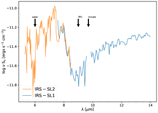
Figure 2: The spectrum from 5 µm to 14 µm from Spitzer IRS after re-reduction. The wavelengths of key spectral features are indicated by arrows.

Figure 2 zooms in on the spectral region from 5 µm to 14 µm. The spectrum is noisy but quite remarkable. The silicate feature is quite shallow for such an embedded source, while the ice features at 6.0 µm and 6.8 µm are very deep. The deepest absorption is around 9.0 µm, a significantly shorter wavelength than the usual maximum absorption by silicate grains. Finally, there seems to be broad absorption over the 13-14 µm region of the water libration mode. This spectrum, while uncertain, is different from all the spectra in Boogert et al. (2008). The fact that we could not do sky subtraction may affect the spectrum. In particular, the shallow silicate feature could arise in part from scattered silicate emission. Improved spectra should be available from approved observations with JWST.

In addition to the SED, we use the radial profiles of emission at 450 µm and 850 µm (Shirley et al. 2000), which are sensitive to the radial variation in the density and hence the evolutionary stage. These profiles provide the strongest constraint on the age of the system.

2.4 ALMA data

ALMA data were obtained as part of Cycle 1 project 2012.1.00346.S (PI N. Evans) on 27 April 2014 (UT) in the C32-3 configuration of ALMA Early Science. The details of the observations and data reduction have been described by Evans et al. (2015). In that paper, the primary spectral line targets (HCN, H¹³CN, and HCO⁺ $J=4\rightarrow 3$ lines and CS $J=7\rightarrow 6$ line) were presented and the HCN and HCO⁺ lines were used to detect infalling motions. The clean beam for Cycle 1 was $490\times 440$ mas at $PA=-76\fdg 9$.

Table 2: ALMA Observations

ID	Date	Antennas	B(min)	B(max)	PWV	Notes
			(m)	(m)	(mm)
uid_A002_Xb57bb5_X451	2016-07-17	41	15	1090	0.57
uid_A002_Xb5aa7c_X4c04	2016-07-22	38	15	1090	0.52
uid_A002_Xb5bd46_X1b74	2016-07-23	37	16	1110	0.67	1
uid_A002_Xb5bd46_X2404	2016-07-23	37	16	1110	0.66	2
uid_A002_Xd1daeb_X2e93	2018-09-11	44	15	1213	0.73
uid_A002_Xd21a3a_X1d4a	2018-09-18	47	15	1397	0.67	3

Note. — 1. $>50$% of antennas had phase fluctuations over limit.

2. 18 antennas exceeded limit on phase fluctuations.

3. 18 antennas had high phase rms, but were usable.

ALMA data with higher spatial resolution were obtained with the same frequency set-ups in Cycle 3 (Table 3) as part of project 2015.1.00169.S and Cycle 4 2016.1.00069.S (PI. N. Evans). Six execution blocks were obtained, four in 2016, which did not meet the noise specifications, and two in 2018; when combined, the data met the noise specifications. The properties of the observations are listed in Table 2, including number of antennas, minimum and maximum baselines, and precipitable water vapor (PWV), along with notes on issues. The properties of the lines observed are given in Table 3. The spectral resolution was 122.07 kHz, except for H¹³CN, for which it was 488.28 kHz. The equivalent values of velocity resolution are listed in Table 3.

The data were calibrated and imaged using CASA (McMullin et al. 2007) version 5.4.0. Observations of strong lines were subject to a calibration error when all these data were obtained that could artificially weaken the lines. The effect is roughly equal to the single-dish line temperature divided by the system temperature. The single dish lines (Evans et al. 2005) have temperatures less than 3 K, versus typical system temperatures during the ALMA observations of about 180 K, so the effect of calibration error should be less than 1.7%, negligible given other uncertainties.

Table 3: ALMA Spectral Windows

Transition	Frequency	$\delta v$	$E_{u}$	$A_{ul}$	Sensitivity
	(GHz)	(km s-1)	(K)	(s-1)	(K/(Jy/bm)-1)
(1)	(2)	(3)	(4)	(5)	(6)
CS $J=7\rightarrow 6$	342.88285030	0.107	65.8	8.4${}\times 10^{-4}$	191
H13CN $J=4\rightarrow 3$	345.33976930	0.424	41.4	1.90${}\times 10^{-3}$	214
HCN $J=4\rightarrow 3$	354.50547590	0.103	42.5	2.05${}\times 10^{-3}$	202
HCO+ $J=4\rightarrow 3$	356.73422300	0.103	42.8	3.57${}\times 10^{-3}$	200

Note. — K was determined from the clean beam and frequency for each line.

After learning of the outburst, we separated the 2016 data from the 2018 data and reduced each separately and refer to them as Cycle3-16 and Cycle3-18. The delay between observations was extremely fortuitous as the lines in 2018 were much stronger, consistent with the brightening seen in the WISE data. The description of the data reduction below applies to both sets of data, except when noted.

Images were made with 0$\farcs$025 cells. Briggs weighting with a robust parameter of 0.5 was used and the task tclean used auto-multithresh for the clean mask, typically with 2 to 3 major cycles. As explained in Evans et al. (2015), removal of the continuum in the uv-plane can cause distortions in spectra with both emission and absorption. The lines and continuum were separated after cleaning with the task imcontsub and spectra were extracted with the task specflux with the region defined to be the size and orientation of the continuum source before deconvolution. The continuum was subtracted in the image plane after careful specification of the line-free channels. A separate reduction with the continuum removed in the uv-plane produced nearly identical results, but with a poorer baseline removal. Self-calibration was used on the continuum and applied to the lines. The clean beam for the 2016 data after self-calibration was $200\times 150$ mas at $PA=-74\fdg 1$. The clean beam for the 2018 data after self-calibration was $240\times 190$ mas at $PA=-63\fdg 1$. The sensitivity, denoted $K$ in kelvin-(Jy/bm)^-1 and computed from the beam and frequency for each line, is given in Table 3 for the 2018 data.

The continuum image from the Cycle 1 observations was presented in Evans et al. (2015), showing a compact central source and faint arcs from the outflow cavity. The Cycle 3 data with better spatial resolution showed many lines of complex organic species, which are presented in a separate paper. They and the main target lines were avoided in constructing the continuum image in Figure 3.

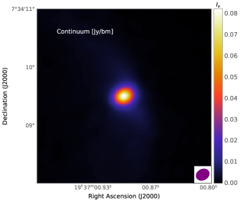
Figure 3: The continuum image from the ALMA Cycle 3 2018 data. The beam is indicated in the lower right corner.

Table 4: ALMA Source Properties

Dataset	MJD	$\theta_{max}$	$\theta_{min}$	PA	$I_{\nu}$	$S_{\nu}$ (fit)	$S_{\nu}$ (2″)	Species
		(mas)	(mas)	(degree)	(mJy/bm)	(mJy)	(mJy)
Cycle1	56774	$491\pm 49$	$258\pm 59$	$9.6\pm 10.1$	$55.1\pm 2.7$	$93.5\pm 6.7$	$110\pm 12$	Cont.
Cycle3-16	57586	$100.1\pm 7.2$	$97.3\pm 8.3$	$43\pm 79$	$89.6\pm 1.0$	$118.5\pm 2.0$	$160\pm 8$	Cont.
Cycle3-18	58379	$186.0\pm 19$	$179\pm 22$	$175\pm 79$	$75.3\pm 2.0$	$129.8\pm 5.1$	$217.5\pm 8.6$	Cont.
Cycle3-18	58379	$789\pm 54$	$467\pm 34$	$72.1\pm 5.3$	$2.75\pm 0.16$	$24.8\pm 1.6$	$28.82\pm 0.63$	HCO+
Cycle3-18	58379	$259.3\pm 9.6$	$228.3\pm 34$	$103\pm 16$	$6.45\pm 0.11$	$14.51\pm 0.33$	$16.83\pm 0.86$	HCN
Cycle3-18	58379	$188.6\pm 10.7$	$156.0\pm 8.8$	$122\pm 17$	$6.04\pm 0.11$	$9.64\pm 0.27$	$8.04\pm 0.72$	H13CN
Cycle3-18	58379	$305\pm 26$	$238\pm 19$	$119\pm 19$	$1.658\pm 0.072$	$3.89\pm 0.23$	$5.31\pm 0.24$	CS

Note. — For the lines, the units are mJy-km s^-1or mJy/bm-km s^-1.

The J2000 peak position for continuum emission, averaged between 2016 and 2018, is 19:37:00.8967, $+$07:34:09.517 with a difference of only 50 mas, consistent within uncertainties with the Cycle 1 peak position. The deconvolved FWHM major and minor axes, peak intensity, and total flux based on an elliptical Gaussian fit are given in Table 4. In addition, we tabulate the total flux density within a 2″ circular area, representing the flux density arising from a region of diameter 329 au.

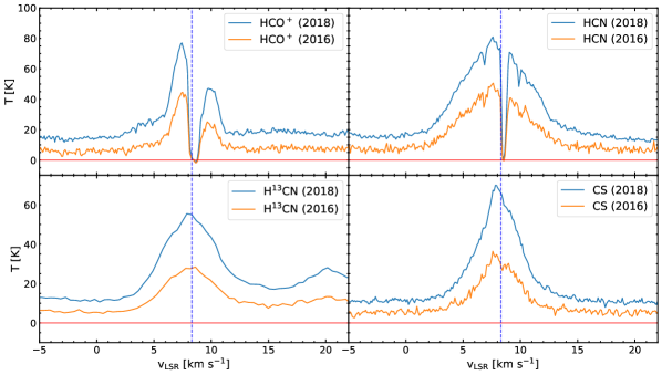
Figure 4: Spectra of the HCO⁺, HCN, CS, and H¹³CN lines in an 0$\farcs$2 diameter circle centered on the continuum source for both the 2016 and 2018 data before the continuum was removed in the image plane. The source velocity is shown as a vertical dashed line.

The spectra of the four lines (Figure 4) from the 2016 and 2018 ALMA data, in an 0$\farcs$2 diameter aperture before removal of the continuum in the image plane, show that the absorption of the continuum by the HCO⁺ and HCN lines is essentially complete and clearly shifted to the red of the source velocity of 8.3 km s^-1 (Evans et al. 2005). The HCN transition has hyperfine structure (Ahrens et al. 2002; Mullins et al. 2016), but 96% of the line strength lies in three hyperfine components within 0.14 km s^-1 of the center frequency that we use to assign velocities. There are two very weak components (2% each) at $+1.34$ km s^-1 and $-1.67$ km s^-1. H¹³CN also has hyperfine structure (Fuchs et al. 2004); again, 96% of the line strength lies within $0.11$ km s^-1of our center frequency, with very weak (2%) features at $+1.39$ km s^-1 and $-1.72$ km s^-1. The peak at velocities below the blue dip in the HCN spectrum is at 6.6 km s^-1, close to the offset expected for the very weak hyperfine component, but the corresponding velocity for the other weak hyperfine component (9.6 km s^-1) corresponds only to the shoulder to the blue of the red dip, not to the secondary peak. No dips or secondary peaks are visible in the H¹³CN spectrum, but some shoulders could plausibly be related to the weak hyperfine components.

The CS line shows a local dip near 8.3 km s^-1, but not absorption below the continuum at the source velocity, while the H¹³CN peaks at the source velocity. The rise at high velocities in the H¹³CN spectrum is caused by lines of COMs, which also partly contribute to the H¹³CN line profile, along with a possible contribution from a line of SO₂ at 356755.19 MHz. The smoother line profile of the H¹³CN observations results from the lower spectral resolution chosen for that band. There are additional dips in the HCN spectrum at $6.9$ km s^-1 and $9.9$ km s^-1.

For comparison to models, the continuum was removed, choosing line free channels to fit the continuum. First order baselines were used, except for H¹³CN and HCN, for which there were too few line-free regions, so a zeroth order baseline was used. We also removed the continuum in the uv-plane for images of the extended emission, and these images are used for some purposes.

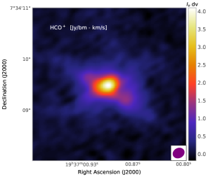
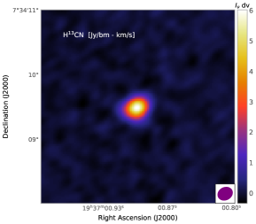
Figure 5: The HCO⁺, HCN, H¹³CN, and CS integrated intensity images from the ALMA Cycle 3 2018 data. The velocity intervals for integration were 1-14 km s^-1 for HCO⁺, $-3$ km s^-1 to 21 km s^-1 for HCN, and 1-12 km s^-1 for H¹³CN, and 1 to 17 km s^-1 for CS. The beam is indicated in the lower right corner.

The intensity, integrated over the line, is shown in Figure 5. The presence of other lines required tuning of the velocity interval, as indicated in the caption. The integrated intensity maps were fitted to Gaussians, and the fitted peak positions were the same for all lines to within 0$\farcs$04, or 20% of the beam size. The average peak position of the lines agreed with that of the continuum to 0$\farcs$025, about 10% of the beam size. The fits were all compact, but they had different sizes, as indicated in Table 4. Except for HCO⁺, they are compact ellipses. The integrated intensity map of HCO⁺ shows extensions likely to be the edges of the outflow cavities in addition to the compact ellipse.

2.5 Outflow Structures

In addition to the spectra toward the continuum source, the ALMA Cycle 3 data reveal some interesting features about the outflow cavity. Partial arcs can be seen in several lines/velocities, but the outflow is prominent in neither the integrated intensity images nor in channels centered on outflow velocities. The most complete image of the cavity walls is that of the CS $J=7\rightarrow 6$ transition at $v=8.24$ km s^-1, as shown in Figure 6. We interpret these arcs as the limb-brightened top and bottom of the cavity walls because the velocity is close to the rest velocity and both blue and red lobes are clearly visible. The structure in Figure 6 is similar to the polarized continuum intensity at 0.87 mm in figure 1 of Yen et al. (2020) but shows the west lobe more clearly. This structure is visible in all three epochs, but it is most prominent in the 2018 data.

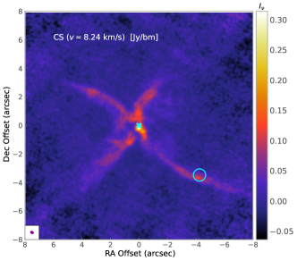
Figure 6: The CS image at $v=8.24$ km s^-1 from 2018. The cavity walls are most apparent at this velocity and this molecular transition. The image is taken from the data with the continuum removed in the image plane. The beam is indicated in the lower left corner.

In the south-western cavity wall, there is a bright knot visible in Figure 6. The HCN spectrum taken at this position (Figure 7) shows a long tail of emission extending about 17 km s^-1 to the red, so we refer to it as the “red blob.” This feature is again seen in all three epochs. None of the other lines show any unusual line profiles at this position. The position of the red blob is $5\farcs 5=910$ au SW of the protostar. An ejection traveling at 100 km s^-1 would take about 46 yr to travel this distance.

Figure 7: The HCN line spectrum of the red blob from Cycle 3, 2018 data. The spectrum was extracted from an ellipse of dimension 0$\farcs$6 by 0$\farcs$3 centered at 19:37:00.611, 07:34:06.05 (J2000).

3 Models of the Dust Continuum Emission

3.1 Luminosity Variation

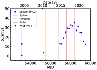
Figure 8: WISE W2 photometry as a function of MJD (C-H Kim et al. in prep.). The vertical lines show the dates of various observations. The red lines indicate Band 7 observations from Cycle 1 and two dates for the Cycle 3 data presented here. The dates of the Spitzer and Herschel observations are indicated by magenta and orange lines, respectively. The likely earliest date for the ejection of the molecular bullet is indicated by the green line.

The light curve of the W2 (4.5 µm) flux densities in Figure 8, along with vertical lines indicating the dates of the Spitzer, Herschel, and selected ALMA observations, implies that the luminosity of B335 increased substantially after about MJD 56000 and has since declined. The Spitzer data were obtained before the original WISE data were available, but the Herschel data were obtained close in time to the original WISE data point, clearly preceding the luminosity rise. We will assume that the Herschel data were also in what we will call the quiescent phase and produce a source model for that phase. Then, we will vary the luminosity in that model to predict the W2 data. After fitting the result, we will have a model for the luminosity as a function of time for the period covered by the W2 data.

3.2 1D Models

The continuum emission from B335 has been extensively modeled (Shirley et al. 2002, 2011; Stutz et al. 2008) but those predating 2008 assumed a distance of 250 pc. Spherical models of inside-out collapse (Shu 1977) are characterized by a sound speed ($c_{{\rm s,eff}}$) and an age ($t_{\rm col}$) since the collapse began. For practical purposes inner and outer radii of the envelope are also assumed. Preliminary versions of these models for the ALMA data were discussed by Evans et al. (2015).

Models of the continuum were compared to photometry (Table 1) and radial profiles at 450 µm and 850 µm emission (Shirley et al. 2002). These 1D models all had two serious problems. Very young ages ($\mbox{$t_{\rm col}$}<1\mbox{${}\times 10^{4}$}$ yr) were required to approximate the radial profiles, but these ages were incompatible with both outflow ages and ages based on modeling line emission. Also, 1D models severely underestimate the observed SED at shorter wavelengths, a well-known problem because such models have too much extinction at short wavelengths (Shirley et al. 2002). A 1D model of a spherical envelope for $\mbox{$t_{\rm col}$}=5\mbox{${}\times 10^{4}$}$ yr is compared to the observations in Figure 9. While the model can reproduce most of the far-infrared and submillimeter data, it severely underproduces the near-infrared data, and the radial profiles are far too flat to match the observations (Figure 10).

Figure 9: Data and 1D model of the SED for spherical collapse at an age of $5\mbox{${}\times 10^{4}$}$ yr. The data are the same as in Figure 1, and the blue open circles are the predictions for the large beam photometry in Table 1.

Figure 10: Observed and modeled radial profiles for spherical collapse at an age of $5\mbox{${}\times 10^{4}$}$ yr. The data are plotted with orange errorbars, and the blue circles are the model predictions.

3.3 3D Models

More realistic models must consider the three-dimensional structure of the source, especially the role of the outflow (Dunham et al. 2010; Yang et al. 2017). We adopted a model that includes an infalling, rotating envelope, an embedded disk, and bipolar outflow lobes. We use the radiative transport code, HYPERION, an open-source, parallelized three-dimensional code (Robitaille 2011). The convergence criteria for HYPERION are applied to the absorption rate ($\dot{A}$) of the dust in each cell. The convergence criteria for most simulations were set so that 95% of the differences between iterations were less than a factor of 2, and the 95% value of the differences changed by less than 1.02 (about 2%).

Table 5: Model parameters

Envelope parameters
$t_{\rm col}$	Age of the protostellar system after the start of collapse.
$c_{{\rm s,eff}}$	Effective sound speed of initial model.
$\mbox{$\Omega_{0}$}^{\rm a}$	The initial angular speed of the cloud.
$\mbox{$r_{\rm out}$}^{\rm a}$	Outer radius of the envelope
Disk parameters
$M_{\rm disk}$	Total mass of the disk.
$\beta$	The flaring power of the disk.
$h_{\rm 100}$	The disk scale height at 100 au.
Outflow cavity parameters
$\mbox{$\theta_{\rm cav}$}^{\rm a}$	The cavity opening angle
$\rho_{\rm cav,0}$	The dust density of the inner cavity.
$R_{\rm cav,0}$	The radius where the cavity density starts to decrease.
$\mbox{$\theta_{\rm incl}$}^{\rm a}$	The inclination angle of the protostar, 0∘ for face-on and 90∘ for edge-on view.
Stellar parameters
$\mbox{$T_{\star}$}^{\rm a}$	The temperature of the central protostellar source assuming blackbody radiation.
$R_{\star}$	The radius of the central protostellar source.
aThese parameters are fixed in the search of the best fit model.

Our modeling approach follows that of Yang et al. (2017), who explained the basic method and explored the effect of the different parameters on the observed SED. We summarize the input model construction here. All the parameters are summarized in Table 5. The envelope is a rotating, infalling envelope that was originally spherical and isothermal (Terebey et al. 1984), the TSC model. This model is defined primarily by the effective sound speed ($c_{{\rm s,eff}}$), the age since collapse began ($t_{\rm col}$), and the initial angular velocity ($\Omega_{0}$). In addition, we specify the outer radius for the envelope ($r_{\rm out}$). The inner radius ($r_{\rm in}$) is set by the dust evaporation temperature in an iterative way. The physical model is axisymmetric, so 2D, but the inclination angle adds a dimension, so the radiative transfer is done in 3D.

Because of the observational constraints on disk size (Yen et al. 2011, 2015a), the disk is not very significant in producing the observed SED, but we model it as a flared disk with parameters described by Yang et al. (2017). The disk is specified by its mass ($M_{\rm disk}$), flaring power-law ($\beta$), and scale height at 100 au ($h_{\rm 100}$). These parameters do affect the near-infrared ($3.6-8$ µm) part of the SED.

We do not model the outflow itself, but only the effect of the cavity on the SED and radial profiles. The outflow lobes are characterized by their shape and the density structure inside them. The shape is defined in cylindrical coordinates, ($z$ and $\varpi$), where $z$ expresses the distance along the outflow axis and $\varpi$ measures the perpendicular distance from that axis to the edge of the lobe. The equation of the surface is $z=c_{0}\varpi^{1.5}$, where

$$c_{0}=\frac{\cos\mbox{$\theta_{\rm cav}$}}{r^{0.5}_{\rm fid}\sin^{1.5}\mbox{$\theta_{\rm cav}$}},$$ (1)

and $\theta_{\rm cav}$ is the half-angle of the outflow lobe measured at $r_{\rm fid}=\mbox{$10^{4}$}$ au, where $r^{2}=\varpi^{2}+z^{2}$. This model produces a curved shape that is qualitatively similar to the shape seen faintly in the Cycle 1 ALMA continuum data (Evans et al. 2015) and in Figure 6. The mass inside the outflow cavity is characterized by a small region of constant density ($\rho_{\rm cav,0}$) that extends out to a radius ($R_{\rm cav,0}$) beyond which the density declines as a power-law ($\rho\propto r^{-2}$). The axis of the outflow is assumed to be aligned with the rotation axis. Finally, the inclination angle of the rotation and outflow axes relative to the line of sight ($\theta_{\rm incl}$) has to be specified. A face-on rotation axis has $\mbox{$\theta_{\rm incl}$}=0$.

In HYPERION  the luminosity source is characterized by a stellar radius ($R_{\star}$) and temperature ($T_{\star}$). For deeply embedded sources, these are nearly degenerate, and only the stellar luminosity ($L_{\star}$) is relevant. We kept $T_{\star}$ fixed and varied $R_{\star}$ to change the luminosity. The actual luminosity arises from accretion, so these parameters are not meant to be realistic. The value of $T_{\star}$ affects the near-infrared portion of the SED somewhat.

The standard dust model is that of column 5 of table 1 of Ossenkopf & Henning (1994) as extended to shorter wavelengths with anisotropic scattering by Young & Evans (2005). The standard Henyey-Greenstein model (Henyey & Greenstein 1941) for the angular distribution of scattering is used, unless otherwise noted.

Table 6: Best-Fit Model parameters

Envelope parameters
$t_{\rm col}$	40000 years
$c_{{\rm s,eff}}$	$0.30~{}{\rm km~{}s}^{-1}$
$\Omega_{0}$	$2.0\times 10^{-14}~{}{\rm s}^{-1}$	(fixed)
$r_{\rm out}$	$2\mbox{${}\times 10^{4}$}$ au	(fixed)
Disk parameters
$M_{\rm disk}$	$0.063$	(fixed)
$\beta$	1.3
$h_{\rm 100}$	4.0 AU
Outflow cavity parameters
$\theta_{\rm cav}$	$27.5^{\circ}$	(fixed)
$\rho_{\rm cav,0}$	$4\times 10^{-20}~{}\rm{g~{}cm}^{-3}$
$R_{\rm cav,0}$	20 AU
$\theta_{\rm incl}$	$87^{\circ}$	(fixed)
Stellar parameters
$T_{\star}$	7000 K	(fixed)
$R_{\star}$	1.17 $\rm R_{\rm\odot}$

Given the very large number of parameters in a 3D model, it is necessary to constrain as many as possible from existing information. The values of parameters that were fixed in the models are listed in Table 6 with a note that they were fixed. The distance was fixed at 164.5 pc (Watson 2020). The initial angular velocity, $\Omega_{0}$, is set at 2${}\times 10^{-14}$ s^-1, based on the arguments in Yen et al. (2019), as noted in §1. The outer radius, $r_{out}$, is set at 2${}\times 10^{4}$ au, about half the estimate from Herschel, but larger radii did not change the results. The mass enclosed in that value of $r_{out}$ is 3.3 M_⊙. The opening angle ($\theta_{\rm cav}$) was set to 27$\fdg$5, based on analysis of the CO outflow in the context of detailed source models (Shirley et al. 2011) and CO maps by Stutz et al. (2008). Most models assumed $\mbox{$\theta_{\rm incl}$}=87\mbox{${}^{\circ}$}$, based on best fits to the SED by Stutz et al. (2008) using model grids and a fitter (Robitaille et al. 2006, 2007).

The values of other parameters are the result of the optimization of the predicted SED and the radial profiles. As discussed at length in the appendix of Yang et al. (2017), the radial profiles and different regions of the SED best constrain different parameters. To compare the model predictions to the observations, a simulated SED was produced by calculating an emission image at a particular wavelength, using the ray-tracing part of HYPERION, and convolving that image with a top hat aperture of the specified size. Azimuthally averaged radial profiles were also computed from the model after simulating the beam used for the observations. Images of the model at specific wavelengths can also provide constraints. We will describe the steps used to optimize the model parameters in the order that they were taken, but the final optimization involves iteration between correlated parameters.

First the luminosity has to be constrained. In the context of these models, a blackbody star is assumed. The stellar parameters of temperature ($T_{\star}$) and radius ($R_{\star}$) enter in combination ($L\propto\mbox{$T_{\star}$}^{4}\mbox{$R_{\star}$}^{2}$). To match the observed luminosity of 1.36 L_⊙ with $\mbox{$\theta_{\rm incl}$}=87\mbox{${}^{\circ}$}$, the central luminosity must be 2.95 L_⊙, 2.2 times the observed luminosity. This result is a feature of models with outflow cavities, which cause the radiation to be channeled through the outflow lobes, and the effect is large in B335 because the outflow is nearly edge-on.

Second, the total mass of the envelope is best constrained by the longest wavelength photometry, given a model of dust opacities. In Shu-type models, this is set by the sound speed ($c_{{\rm s,eff}}$) because the density depends on the sound speed: $\rho=\mbox{$c_{{\rm s,eff}}$}^{2}/(2\pi Gr^{2})$. The new, larger distance necessitated some changes in parameters used in recent modeling (Evans et al. 2015). The effective sound speed, including turbulence, $c_{{\rm s,eff}}$ had been taken to be $0.233$ km s^-1 (Evans et al. 2015) in models of the source at 100 pc distance. At the larger distance, a larger sound speed is needed to match the flux into large beams at the longest wavelengths, with a value of $\mbox{$c_{{\rm s,eff}}$}=0.30$ km s^-1 working well. The previous value was obtained by adding in quadrature the thermal sound speed for an initial $\mbox{$T_{K}$}=13$K (Evans et al. 2005) and the microturbulent contribution inferred from line widths in single-dish beams (Evans et al. 2015). The obvious justification for increasing $c_{{\rm s,eff}}$ is that the Alfven speed has not yet been included. If added in quadrature (Shu et al. 1987), the required Alfven speed would be $0.19$ km s^-1. The Alfven speed is $B(4\pi\rho)^{-0.5}$. The large scale magnetic field is estimated at $30.2\pm 17.7$ $\mu$G (Kandori et al. 2020) but the relevant, pre-collapse density is unclear in the presence of a density gradient. The required Alfven speed can be obtained if the relevant density is about $5\mbox{${}\times 10^{4}$}$ cm^-3, a very reasonable value. Zielinski et al. (2021) derived a field value of $142\pm 46$ $\mu$G from observations at 214 µm and an assumed density of $\rho=5.41\mbox{${}\times 10^{-18}$}$ g cm^-3. This combination leads to nearly the same Alfven speed of $0.17$ km s^-1. The change in $c_{{\rm s,eff}}$ leads to changes in many other derived properties compared to previous models (Evans et al. 2015). These will be summarized in §5.2 after the other modeling parameters are discussed.

Third, the age of the source must be constrained. In TSC models, the age is the time elapsed since the initiation of infall ($t_{\rm col}$). The age and sound speed determine the infall radius ($\mbox{$r_{\rm{inf}}$}=\mbox{$c_{{\rm s,eff}}$}\mbox{$t_{\rm col}$}$), which determines the shape of the density profile. In turn, the density profile is the main determinant of the normalized, azimuthally averaged, radial profile of emission at submillimeter wavelengths (i.e., the radial profile). As the source evolves, the initial $\rho\propto r^{-2}$ density profile shifts to a flatter profile, leading to a flatter predicted radial intensity profile (Fig. 25 of Yang et al. 2017). Since we have adjusted $c_{{\rm s,eff}}$ in the second step, we vary $t_{\rm col}$ to best approximate the observed radial intensity profiles. The observed radial profiles are annular averages, so we produce the model radial profiles in the same way, thus accounting for the effect of the outflow cavity. Models with different $t_{\rm col}$ are compared to the observations in Figure 11. The radial profile at 450 µm is best matched at $\mbox{$t_{\rm col}$}=5\mbox{${}\times 10^{4}$}$ yr, but the profile at 850 µm, which is less sensitive to the temperature distribution, favors $\mbox{$t_{\rm col}$}=3\mbox{${}\times 10^{4}$}$ yr. An age of $4\mbox{${}\times 10^{4}$}$ yr predicts a radial profile at 850 µm that is slightly too flat and one at 450 µm that is slightly too steep, thus presenting about the best compromise. The larger distance and larger $c_{{\rm s,eff}}$ partially cancel out in their effects on the radial intensity profiles of the model, so that the best-fit $\mbox{$t_{\rm col}$}=4\mbox{${}\times 10^{4}$}$ yr is not very different from the age of 5${}\times 10^{4}$ yr favored by Evans et al. (2015). We adjusted $M_{\rm disk}$ to be 0.25 of the collapsed mass ($\mbox{$M_{\star}$}+\mbox{$M_{\rm disk}$}$) because larger ratios tend to be unstable. For the age and infall rate fixed by the above considerations, $\mbox{$M_{\star}$}=0.25\ \mbox{M${}_{\odot}$}$, so $\mbox{$M_{\rm disk}$}=0.063\ \mbox{M${}_{\odot}$}$. For comparison, Evans et al. (2015) set a limit on the optically thin mass based on the Cycle 1 data; after updating to the new distance, the limit would be about 2${}\times 10^{-3}$ M_⊙. However, our modeling shows that much larger disk masses can be hidden by optically thick dust in the small disk of our models.

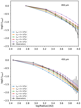
Figure 11: Observations and 3D model of the radial profile of the submillimeter wavelength emission. Models with $\mbox{$t_{\rm col}$}=3\mbox{${}\times 10^{4}$}$ yr, $\mbox{$t_{\rm col}$}=4\mbox{${}\times 10^{4}$}$ yr, $\mbox{$t_{\rm col}$}=5\mbox{${}\times 10^{4}$}$ yr, and $\mbox{$t_{\rm col}$}=8\mbox{${}\times 10^{4}$}$ yr are shown.

Fourth, the mid-infrared part of the SED is most affected by the cavity properties, especially the density at the base of the cavity, with some effects from the disk properties. The best match was found for a radius for the region of constant density in the cavity ($R_{\rm cav,0}$) of 20 au, and the density of the constant region ($\rho_{\rm cav,0}$) of 4${}\times 10^{-20}$ g cm^-3. However, these parameters also affect the SED at shorter wavelengths because the flux densities at those wavelengths are dominated by light scattered from the outflow cavity. The density that produces enough emission at 24 µm somewhat overproduces the emission in the small apertures in the IRAC bands, unless the disk and star parameters can compensate.

The near-infrared part of the SED (the IRAC bands) depends on many parameters, including the rotation rate, inclination angle, cavity properties, disk properties, and stellar properties. Deviations from the assumed simple, azimuthally symmetric structure can also have a big effect, so a good fit to the IRAC flux densities cannot necessarily be interpreted as actually representing the structure. With that caveat in mind, we describe the adjustments used to provide a decent match to the near-infrared observations. A lower $T_{\star}$, with the larger $R_{\star}$ needed to maintain the luminosity, produced more emission in the near-infrared. A better match was found for the (rather unrealistic) value of $\mbox{$T_{\star}$}=7000$ K. We produced small grids of $\Omega_{0}$, $\theta_{\rm incl}$, $\beta$ and $h_{\rm 100}$ to optimize the near-infrared SED. The resulting best-fitting parameters are listed in Table 6. The common feature of these best parameters is that they minimize the emission in the IRAC bands. Some of the parameters are not very realistic. $T_{\star}$ is quite large for a star of 0.25 M_⊙, and the disk parameters ($\beta$, $h_{\rm 100}$) produce a very flat disk. Even with these rather extreme parameters, the IRAC fluxes into small apertures are over-produced, especially at 3.6 µm. More typical stellar and disk parameters could be used if there is an extra source of extinction near the source, as will be discussed below.

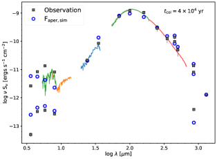
Figure 12: Observations and best 3D model of the continuum SED, with the parameters in Table 6.

The SED of the best model for the continuum is shown in Figure 12. The SED is well matched except in the near-infrared, where the model over-predicts the emission into small beams and under-predicts the emission into large beams, and the ALMA observations, which we discuss below. At 3.6 µm, the model strongly over-predicts the emission into both large and small beams. Variations in the disk, cavity, and stellar properties were used to optimize the near-infrared, but the over-prediction into small beams was a robust result. The 3D models produce a much better (though still imperfect) match to the short wavelength emission than did the 1D model with the same age. The outflow cavity has clearly allowed more radiation at mid-infrared and near-infrared wavelengths to reach the observer. The emission is essentially all scattered by the outflow cavities into the line of sight.

Figure 13: Image at 4.5 µm based on the continuum model with parameters in Table 6. .

Figure 13 shows a simulated image at 4.5 µm; two fan-shaped nebulosities, strongly peaked near the source and brighter along the cavity wall, are clearly seen. The shape agrees well with the image of the cavity walls indicated by the CS emission (Figure 6) and roughly with the image in Figure 9 of Stutz et al. (2008), but the model is more symmetric between the two lobes than are the infrared observations.

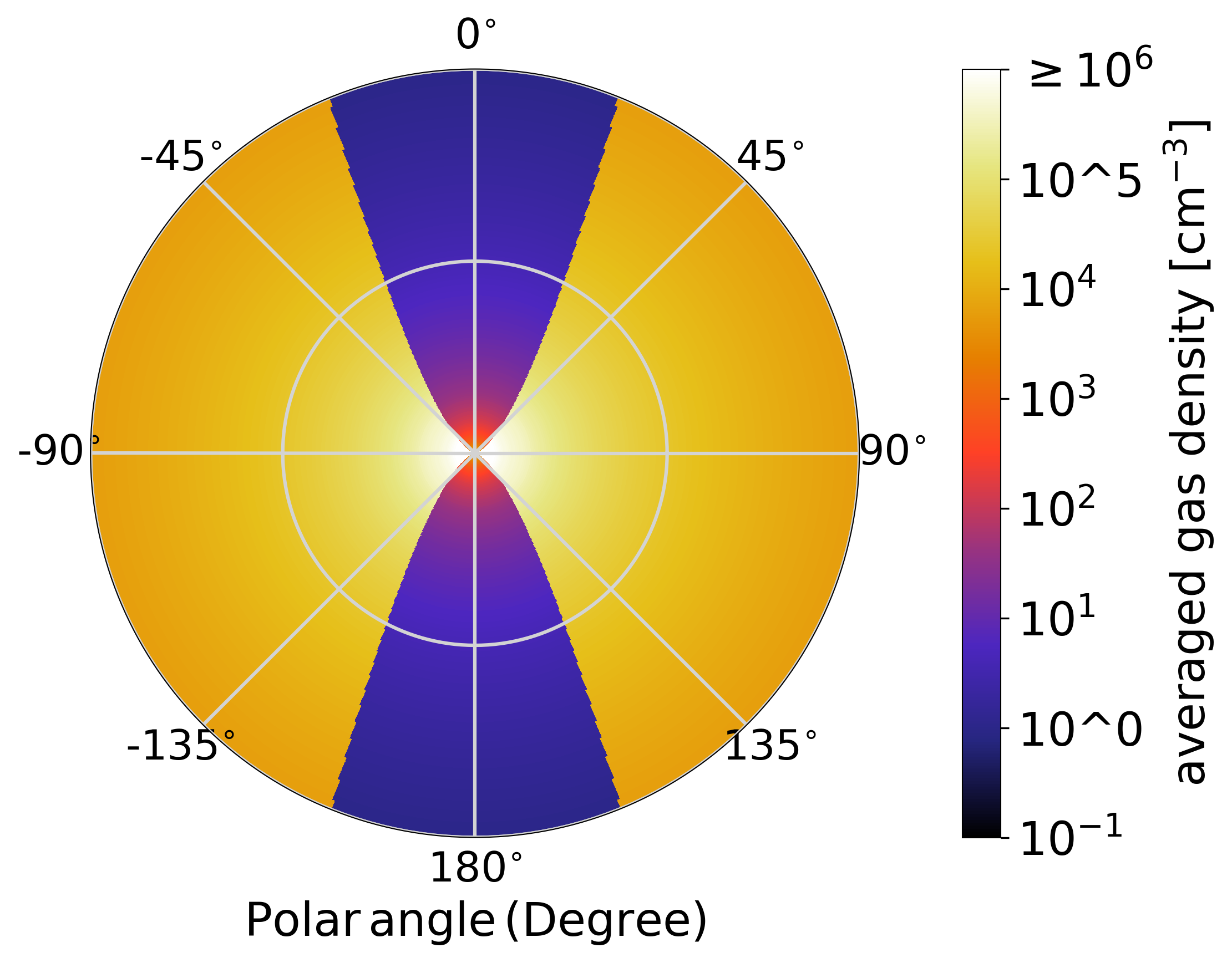
Figure 14: The distribution of average gas density as a function of radius and polar angle. Note that the model polar angle is taken relative to the z axis. For comparison to data, we rotate the model predictions to the E-W outflow direction.

The density structure of the best-fitting model is shown in Figure 14, which also defines the polar angle of the model, $\theta$. The model has the outflow cavities along the z axis by convention, so this image is rotated by 90 degrees from the one in Figure 13. The radial distributions of dust density along five distinct polar angles are shown in Figure 15. The sharp increases show when the line of sight passes from the cavity into the envelope.

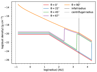
Figure 15: The radial distribution of dust density at five different polar angles, as defined in Figure 14. Except for $\theta=90\mbox{${}^{\circ}$}$, the profiles start in the cavity and increase sharply at the radius where the line-of-sight passes out of the cavity into the envelope.

One glaring failure of the continuum model is the weakness of the emission predicted for the ALMA emission into a 2″ aperture. The best model predicts a flux that is a factor of 3 less than the Cycle 1 observations. Even the Cycle 1 observations may have occurred after the beginning of the rise in luminosity, and the continuum flux increases by a factor of 2 by the time of the 2018 observations. However, models with higher luminosity also fail to reproduce the ALMA data at any of the three epochs. A wide range of parameters for the disk, $\Omega_{0}$, etc. were tried, but the predicted emission into a 2″ aperture was rather insensitive to these variations and was never close to the observed emission.

To compare to the ALMA data in more detail, a model image was made at the mean wavelength of the ALMA data and converted into uv-plane data using the CASA task simobserve for the Cycle 1 data. Then simanalyze was used to create an ALMA image which was fitted with an elliptical Gaussian within a 2″ circle. The emission in the model has a lower peak intensity and is much more elongated than the observed emission, being defined by the outflow cavity walls. So, neither the shape nor the flux are reproduced well. A similar issue was seen in BHR71 by Yang et al. (2020), who suggested the presence of an additional structure between the envelope and the Keplerian disk. The ALMA continuum data strongly suggest that there is a structure on the scales of $\sim 30$ au in addition to the envelope and disk in our models. Such a structure could also provide additional extinction at short wavelengths, as suggested above in the discussion of the discrepancies in the near-infrared. The most likely candidate is something like a pseudo-disk, but a thermal radio jet could also contribute. Purser et al. (2016) found spectral indices as high as 1.6 in their study of radio jets from 5 to 23 GHz. If such a large index persisted to 345 GHz, the largest flux found by Galván-Madrid et al. (2004) could account for all the continuum that we observe. For a more typical index of 0.3, the contribution would be negligible.

In summary, 3D models with outflow cavities can reproduce observations of both the radial profile and most of the SED with TSC models of reasonable ages ($\mbox{$t_{\rm col}$}=3-5\mbox{${}\times 10^{4}$}$ yr). The outflow cavities are the critical element in resolving issues found in 1D models.

3.4 Luminosity Variation

With a model for the quiescent source, we can relate the W2 photometric variation to variations in the luminosity. We ran a series of models, changing only the stellar radius (a stand-in for central luminosity), each predicting the W2 photometry. Then the relation between the model luminosity and the W2 flux density from the model was fitted with a quadratic function between about 3 L_⊙ and 25 L_⊙. The best-fitting model was

$$L/\mbox{L${}_{\odot}$}=1.837+0.845S_{\nu}(W2)+0.001S_{\nu}(W2)^{2}$$ (2)

with $S_{\nu}(W2)$ the WISE photometry in mJy. The actual photometry as a function of time, multiplied by a factor of 0.67 to account for a slight under-prediction by the models, then allows a model for the central luminosity as a function of time (Figure 16). This model predicts a luminosity increase of a factor of 5-7 over the quiescent state.

Figure 16: The central luminosity as a function of time based on modeling the WISE W2 photometry. The vertical lines are the same as in Figure 8.

In principle, the W1 photometry might be preferred because the W2 bandpass includes likely strong line emission from H₂ and CO (Yoon et al. 2022), . However, our model for the W2 emission matches the observations better than it does for the W1 bandpass. Time sequence far-infrared photometry is what is really needed. There is one useful data point at 214 µm for MJD 58044, near the peak luminosity (Zielinski et al. 2021). Our luminosity model predicts $L\approx 20$ L_⊙ at that date, but the 214 µm flux density is better matched in a model with $L\approx 6$ L_⊙. There will be a time delay before the luminosity burst covers the full region that contributes to the far-infrared emission into relatively large beams (Francis et al. 2022), which would imply a luminosity larger than 6 L_⊙ at the time of the 214 µm observations. Consequently, the actual increase is rather uncertain, but likely a factor between 5 and 7.

4 Models of Line Emission

4.1 3D Models

To see how 3D models with outflow cavities and the small amount of rotation seen in B335 would fare, we used LIME (Brinch & Hogerheijde 2010) to model the line emission from the models computed for the dust emission with HYPERION. Because our dust model underestimates the ALMA observations, we also used a custom code (LIME-AID) to add a continuum source at the center of the model equal to the observed flux density (Yang et al. 2020). We used $5\mbox{${}\times 10^{4}$}$ intensity grid points (pIntensity) for running models, but doubled that to $1\mbox{${}\times 10^{5}$}$ for the final models. Using twice the number produced slightly smoother spectra, but the differences were very minor.

The spectral line models used the density and velocity fields from the TSC models, supplemented by the cavities added to model the continuum emission. In the inner regions, the gas temperature was assumed equal to the dust temperature from the HYPERION models, including the cavities, so the temperature is higher around the cavities. For radii larger than 2600 au, the gas temperature was increased, based on the models including gas heating by photoelectric heating by the interstellar radiation field (Fig. 8 of Evans et al. 2005). Because the adaptive gridding used by LIME was unduly distorted by the sharp discontinuity of the outflow cavity, we did not use the particle volume density inside the cavity of the continuum models, but instead set the abundance of the species being modeled to zero inside the cavity. The higher temperatures near the cavity were captured from the continuum models, but there were no changes in the gas velocity, so the outflows were not modeled.

The new variables introduced for the lines are those that characterize the microturbulence and the abundance profile. The microturbulence was taken as $b=0.12$ km s^-1, as in previous models, and assumed to be independent of radius. The rotation was already in the TSC models, but for the line simulation, the sense of rotation matters as well. Based on a map of H¹³CO⁺ $J=1\rightarrow 0$ emission, Kurono et al. (2013) found a velocity gradient from south to north, indicating that the north side is rotating away from us on large scales ($r\sim 2\mbox{${}\times 10^{4}$}$ au). Because the rotation in the models is clockwise as viewed from the “north” pole of the model, the left side of the model is coming towards us and identified with south for comparison to the data,

Chemical models were used to calculate the abundances of species in the envelope at various ages. The chemical model is described in detail in Zhao et al. (2018), so we provide here only a brief description. The network includes 21 neutral species, 31 ionic species, and 500 reactions. Freeze-out and desorption processes are included, but molecular reactions on the grain surface are not. Sulfur, thus CS, is not included in the model. The abundances were calculated for the tenperature and density structure of the envelope at a given time. Rather than following the chemistry through the evolution, the abundances were pre-computed for a range of temperatures and densities at a given chemical time to form a look-up table. The abundances are produced for a range of radii and polar angles. Because the abundances were nearly identical as a function of polar angle, we used the value for 45° for all angles and set the abundance to zero in the outflow cavity. Calculations were available for ages of 1, 3, 4, and 5 times $10^{4}$ yr. The abundances used in the models are shown in Figure 17. These were interpolated onto the grid used by LIME. These models were computed before the luminosity variation was discovered, so they assumed the pre-outburst luminosity.

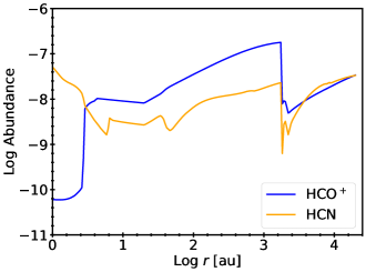
Figure 17: The abundance profile as a function of radius at $\mbox{$t_{\rm col}$}=3\mbox{${}\times 10^{4}$}$ yr from the chemical model for both HCO⁺ and HCN.

We focus first on the HCO⁺ emission, using the ALMA Cycle 1 data (Evans et al. 2015), and the ALMA Cycle 3 2018 data. To simulate the continuum source, we use the LIME-AID code (Yang et al. 2020) and insert a continuum source at the center matching the continuum before deconvolution, as noted above. The position angle was rotated by 90^∘ because the model has the outflow in the north-south direction. Then we convolve the result from LIME-AID to the clean beam used for the data and extract a spectrum in the same way that we used for the data. We focus on ages of 1${}\times 10^{4}$ to 5${}\times 10^{4}$ yr, consistent with the results from the continuum modeling and past experience with the lines.

While many things affect the model line profiles, the clearest effect comes from the age of the system. Figure 18 shows line profiles for HCO⁺ and HCN $J=4\rightarrow 3$ for ages from $\mbox{$t_{\rm col}$}=1\mbox{${}\times 10^{4}$}$ yr to $5\mbox{${}\times 10^{4}$}$ yr. As the collapse proceeds, the infall velocities increase, moving the blue and red peaks apart, the lines broaden, and the self-absorption in the front part of the cloud broadens, eroding the lower velocity emission in the red peak.

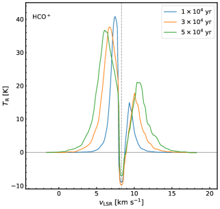
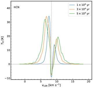
Figure 18: The model $J=4\rightarrow 3$ line profiles for ages from $\mbox{$t_{\rm col}$}=1\mbox{${}\times 10^{4}$}$ yr to $\mbox{$t_{\rm col}$}=5\mbox{${}\times 10^{4}$}$ yr, using the abundances from the chemical models at those ages.

Because of the luminosity variation, we produced models of the line emission for a range of luminosities at fixed age ($\mbox{$t_{\rm col}$}=3\mbox{${}\times 10^{4}$}$ yr). These show that the shape of the HCO⁺ line is little affected by the source luminosity, but the strength increases smoothly with luminosity (Figure 19). Because the chemical models do not include the luminosity variation, these line emission models are not self-consistent.

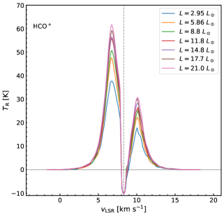
Figure 19: The model HCO⁺  $J=4\rightarrow 3$ line profiles for luminosities from 3 L_⊙ to 21 L_⊙, all for $\mbox{$t_{\rm col}$}=3\mbox{${}\times 10^{4}$}$ yr using the abundances from the chemical models at that age.

To compare models to observations quantitatively, the figure of merit is the absolute value of the difference between observations and models, averaged over $\pm 3$ km s^-1 about the $v_{LSR}$.

$$\mbox{$\langle\mid\rm{Res}\mid\rangle$}=\mbox{$\langle\mid\rm{Obs(v)-Model(v)}\mid\rangle$}$$ (3)

The chemical models have only the single variable of age. Ages of $1-5\mbox{${}\times 10^{4}$}$ yr were tried for both HCO⁺ and HCN. The age of $\mbox{$t_{\rm col}$}=3\mbox{${}\times 10^{4}$}$ yr was clearly best for HCO⁺, but models with $\mbox{$t_{\rm col}$}=4\mbox{${}\times 10^{4}$}$ yr were not much worse. HCN was about equally (poorly) fitted by 3${}\times 10^{4}$ yr and 4${}\times 10^{4}$ yr. The resulting line profiles are shown in Figure 20. The model can reproduce the HCO⁺ Cycle 1 data reasonably. The absorption dip is shifted to the red, matching the observations, but has more absorption near the systemic velocity than the observations. These failings apply to HCN as well, but in addition, the modeled HCN lines lack the broad wings seen in the observations. We are not modeling the outflow, a likely source of the broad wings in the observed HCN line.

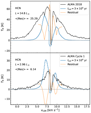
Figure 20: The HCO⁺ $J=4\rightarrow 3$ (left) and HCN (right) line profiles in black from Cycle 3 2018 (top) and Cycle 1 (bottom) with the model for $\mbox{$t_{\rm col}$}=3\mbox{${}\times 10^{4}$}$ yr and the chemical model in blue. The model for the 2018 data assumes $L=14.8$ L_⊙, while that for Cycle 1 assumes $L=2.95$ L_⊙. The difference between observations and model is plotted in orange and the average absolute value of the difference over velocities from $\mbox{$v_{LSR}$}\pm 3$ km s^-1 is indicated in the legend.

For the 2018 data, we clearly need to use a larger source luminosity. Our model based on the W2 photometry indicates $L\approx 20$ L_⊙ when the 2018 data were taken, but this is uncertain as discussed above. We ran a series of models of increasing luminosity (controlled by increasing the stellar radius), while keeping the other variables fixed. The resulting HCO⁺ spectra in Figure 19 show that the line increases in strength as the luminosity increases. The model with $L=15$ L_⊙ matches the 2018 HCO⁺ spectrum best. This luminosity worked best if $\mbox{$t_{\rm col}$}=4\mbox{${}\times 10^{4}$}$ yr as well.

5 Discussion

5.1 Physical Model

The 3D model that fits the dust continuum emission best has the properties in Table 6. Both the SED and the radial profiles are reasonably well reproduced by this physical model with $\mbox{$t_{\rm col}$}=4\mbox{${}\times 10^{4}$}$ yr, though ages of $3-5\times\mbox{$10^{4}$}$ yr are nearly as good. This result is a major improvement over 1D models, which could not match the whole SED and required unrealistically young ages to match the radial profiles. The same basic model, with $\mbox{$t_{\rm col}$}=3\mbox{${}\times 10^{4}$}$ yr, supplied with abundances of HCO⁺ from chemical models, gets the basics of the HCO⁺ observations correct, in particular the separation of the blue and red peaks, which is the main indicator of age. Moving to a 3D model mostly resolved the discrepancy between models of the continuum and models of the lines. The models are, however, not as effective in matching the Cycle 3 data nor the HCN line profile. Overall, models with ages $\mbox{$t_{\rm col}$}=3-4\times\mbox{$10^{4}$}$ yr provide the best fits to both continuum and line data.

5.2 Properties of B335

With the revised distance and best fitting age for the source, we need to update the basic source properties from those given in Evans et al. (2015). The best fitting ages ($\mbox{$t_{\rm col}$}=4\mbox{${}\times 10^{4}$}$ yr from continuum modeling or $\mbox{$t_{\rm col}$}=3\mbox{${}\times 10^{4}$}$ yr from line modeling) are generally consistent with the outflow age of 2${}\times 10^{4}$ yr. We address first the properties of the source before the luminosity increase. The new distance results in an observed luminosity of 1.36 L_⊙; for the adopted inclination angle of 87^∘, the actual central luminosity must be 2.95 L_⊙. The greater distance also required a higher effective sound speed, $\mbox{$c_{{\rm s,eff}}$}=0.30$ km s^-1, leading to a higher mass inside $\mbox{$r_{out}$}=2\mbox{${}\times 10^{4}$}$ au of 3.37 M_⊙. Because the mass infall rate is proportional to $\mbox{$c_{{\rm s,eff}}$}^{3}$, it increases substantially to 6.26${}\times 10^{-6}$ M_⊙ yr^-1. With an age of $\mbox{$t_{\rm col}$}=4\mbox{${}\times 10^{4}$}$ yr (from the continuum model), the total mass that has fallen in would be 0.26 M_⊙. For $\mbox{$t_{\rm col}$}=3\mbox{${}\times 10^{4}$}$ yr (from the line models), it would be 0.19 M_⊙. The latter is more consistent with 0.17 M_⊙ derived by Estalella et al. (2019) (scaled to the new distance) from analysis of the first moment of various observations (the central blue spot analysis), though either is probably consistent, given uncertainties.

For the larger mass of 0.26 M_⊙, the luminosity predicted for the infall rate is $L=43.6f_{acc}$ L_⊙. If the radiative efficiency of accretion $f_{acc}=0.5$, the predicted luminosity is 21.8 L_⊙, close to the peak inferred from modeling the W2 variation. In an episodic accretion picture, the pre-outburst luminosity resulted from an accumulation of mass in an intermediate reservoir, such as a pseudodisk or a Keplerian disk. The luminosity outburst would then represent a “catch-up” to match the rate at which envelope material is infalling.

5.3 Caveats and Future Prospects

While modeling in three dimensions has resolved some puzzles, newer ones are now apparent. The failure of models to reproduce the continuum emission from ALMA suggests the existence of additional components, such as a pseudo-disk or a radio jet with a large positive spectral index. Observations in the 1-10 mm wavelength region would resolve the latter possibility. The constraints based on photometry from 3 to 24 µm should be viewed skeptically in light of deep ice absorptions and strong line emission that are emerging from early observations with JWST (Yang et al. 2022). Contamination of the NEOWISE filters by likely CO ro-vibrational emission, H₂ emission lines, atomic lines and ice absorptions render suspect the modeling of the luminosity variation in the one data set with time-domain observations. Chemical models with varying luminosities combined with the full array of ALMA observations may be able to reconstruct the luminosity history, and JWST spectra will dramatically improve our knowledge of the near-source physical and chemical environment. Future models will need to consider departures from axisymmetry given evidence for infalling streamers.

6 Summary

The combination of data from Spitzer, Herschel, and ALMA, supplemented by data from the literature, provides an extremely detailed set of constraints for models of B335. Models of the continuum emission with rotating, infalling (TSC) envelopes, outflow cavities, and disks can provide a reasonable match to the SED and radial profiles at submillimeter wavelengths for ages ($t_{\rm col}$) of $3-4\mbox{${}\times 10^{4}$}$ yr. Similar ages with chemical models provide the best fit to the HCO⁺ spectra from ALMA. The HCN spectrum is, however, less well-fitted.

B335 has undergone an increase in luminosity over the last few years of a factor of 5-7, but is now decreasing back toward its previous luminosity of about 3 L_⊙. The ALMA observations at various times during this luminosity excursion show strong responses in the line strength with increasing luminosity. There were also pronounced increases in emission from COMs, which will be analyzed in a separate paper.

The revised infall rate predicts a luminosity near the peak of the recent outburst, suggesting that the pre-outburst source was storing matter in a structure between the envelope and the star.

References

- Ahrens et al. (2002) Ahrens, V., Lewen, F., Takano, S., et al. 2002, Zeitschrift Naturforschung Teil A, 57, 669, doi: 10.1515/zna-2002-0806
- Anglada et al. (1992) Anglada, G., Rodriguez, L. F., Canto, J., Estalella, R., & Torrelles, J. M. 1992, ApJ, 395, 494, doi: 10.1086/171670
- Astropy Collaboration et al. (2013) Astropy Collaboration, Robitaille, T. P., Tollerud, E. J., et al. 2013, A&A, 558, A33, doi: 10.1051/0004-6361/201322068
- Astropy Collaboration et al. (2018) Astropy Collaboration, Price-Whelan, A. M., Sipőcz, B. M., et al. 2018, AJ, 156, 123, doi: 10.3847/1538-3881/aabc4f
- Bjerkeli et al. (2019) Bjerkeli, P., Ramsey, J. P., Harsono, D., et al. 2019, A&A, 631, A64, doi: 10.1051/0004-6361/201935948
- Bok & Reilly (1947) Bok, B. J., & Reilly, E. F. 1947, ApJ, 105, 255, doi: 10.1086/144901
- Boogert et al. (2008) Boogert, A. C. A., Pontoppidan, K. M., Knez, C., et al. 2008, ApJ, 678, 985, doi: 10.1086/533425
- Brinch & Hogerheijde (2010) Brinch, C., & Hogerheijde, M. R. 2010, A&A, 523, A25, doi: 10.1051/0004-6361/201015333
- Cabedo et al. (2021) Cabedo, V., Maury, A., Girart, J. M., & Padovani, M. 2021, A&A, 653, A166, doi: 10.1051/0004-6361/202140754
- Choi et al. (1995) Choi, M., Evans, II, N. J., Gregersen, E. M., & Wang, Y. 1995, ApJ, 448, 742, doi: 10.1086/176002
- Chu et al. (2020) Chu, L. E. U., Hodapp, K., & Boogert, A. 2020, ApJ, 904, 86, doi: 10.3847/1538-4357/abbfa5
- Chu & Hodapp (2021) Chu, L. E. U., & Hodapp, K. W. 2021, ApJ, 918, 2, doi: 10.3847/1538-4357/ac0ae8
- Dunham et al. (2010) Dunham, M. M., Evans, Neal J., I., Terebey, S., Dullemond, C. P., & Young, C. H. 2010, ApJ, 710, 470, doi: 10.1088/0004-637X/710/1/470
- Estalella et al. (2019) Estalella, R., Anglada, G., Díaz-Rodríguez, A. K., & Mayen-Gijon, J. M. 2019, A&A, 626, A84, doi: 10.1051/0004-6361/201834998
- Evans et al. (2015) Evans, II, N. J., Di Francesco, J., Lee, J.-E., et al. 2015, ApJ, 814, 22, doi: 10.1088/0004-637X/814/1/22
- Evans et al. (2005) Evans, II, N. J., Lee, J.-E., Rawlings, J. M. C., & Choi, M. 2005, ApJ, 626, 919, doi: 10.1086/430295
- Francis et al. (2022) Francis, L., Johnstone, D., Lee, J.-E., et al. 2022, ApJ, 937, 29, doi: 10.3847/1538-4357/ac8a9e
- Fuchs et al. (2004) Fuchs, U., Bruenken, S., Fuchs, G. W., et al. 2004, Zeitschrift Naturforschung Teil A, 59, 861, doi: 10.1515/zna-2004-1123
- Gaia Collaboration et al. (2016) Gaia Collaboration, Prusti, T., de Bruijne, J. H. J., et al. 2016, A&A, 595, A1, doi: 10.1051/0004-6361/201629272
- Gaia Collaboration et al. (2021) Gaia Collaboration, Brown, A. G. A., Vallenari, A., et al. 2021, A&A, 649, A1, doi: 10.1051/0004-6361/202039657
- Gâlfalk & Olofsson (2007) Gâlfalk, M., & Olofsson, G. 2007, A&A, 475, 281, doi: 10.1051/0004-6361:20077889
- Galván-Madrid et al. (2004) Galván-Madrid, R., Avila, R., & Rodríguez, L. F. 2004, Rev. Mexicana Astron. Astrofis., 40, 31
- Gildas Team (2013) Gildas Team. 2013, GILDAS: Grenoble Image and Line Data Analysis Software. http://ascl.net/1305.010
- Green et al. (2013) Green, J. D., Evans, II, N. J., Jørgensen, J. K., et al. 2013, ApJ, 770, 123, doi: 10.1088/0004-637X/770/2/123
- Green et al. (2016) Green, J. D., Yang, Y.-L., Evans, II, N. J., et al. 2016, AJ, 151, 75, doi: 10.3847/0004-6256/151/3/75
- Henyey & Greenstein (1941) Henyey, L. G., & Greenstein, J. L. 1941, ApJ, 93, 70, doi: 10.1086/144246
- Hirano et al. (1988) Hirano, N., Kameya, O., Nakayama, M., & Takakubo, K. 1988, ApJ, 327, L69, doi: 10.1086/185142
- Imai et al. (2019) Imai, M., Oya, Y., Sakai, N., et al. 2019, ApJ, 873, L21, doi: 10.3847/2041-8213/ab0c20
- Imai et al. (2016) Imai, M., Sakai, N., Oya, Y., et al. 2016, ApJ, 830, L37, doi: 10.3847/2041-8205/830/2/L37
- Jensen et al. (2021) Jensen, S. S., Jørgensen, J. K., Kristensen, L. E., et al. 2021, A&A, 650, A172, doi: 10.1051/0004-6361/202140560
- Kandori et al. (2020) Kandori, R., Saito, M., Tamura, M., et al. 2020, ApJ, 891, 55, doi: 10.3847/1538-4357/ab6f07
- Keene et al. (1983) Keene, J., Davidson, J. A., Harper, D. A., et al. 1983, ApJ, 274, L43, doi: 10.1086/184147
- Kurono et al. (2013) Kurono, Y., Saito, M., Kamazaki, T., Morita, K.-I., & Kawabe, R. 2013, ApJ, 765, 85, doi: 10.1088/0004-637X/765/2/85
- Launhardt et al. (2013) Launhardt, R., Stutz, A. M., Schmiedeke, A., et al. 2013, A&A, 551, A98, doi: 10.1051/0004-6361/201220477
- Lebouteiller et al. (2010) Lebouteiller, V., Bernard-Salas, J., Sloan, G. C., & Barry, D. J. 2010, PASP, 122, 231, doi: 10.1086/650426
- Mainzer et al. (2014) Mainzer, A., Bauer, J., Cutri, R. M., et al. 2014, ApJ, 792, 30, doi: 10.1088/0004-637X/792/1/30
- Maury et al. (2018) Maury, A. J., Girart, J. M., Zhang, Q., et al. 2018, MNRAS, 477, 2760, doi: 10.1093/mnras/sty574
- McMullin et al. (2007) McMullin, J. P., Waters, B., Schiebel, D., Young, W., & Golap, K. 2007, Astronomical Society of the Pacific Conference Series, Vol. 376, CASA Architecture and Applications, ed. R. A. Shaw, F. Hill, & D. J. Bell, 127
- Mullins et al. (2016) Mullins, A. M., Loughnane, R. M., Redman, M. P., et al. 2016, MNRAS, 459, 2882, doi: 10.1093/mnras/stw835
- Okoda et al. (2022) Okoda, Y., Oya, Y., Imai, M., et al. 2022, ApJ, 935, 136, doi: 10.3847/1538-4357/ac7ff4
- Olofsson & Olofsson (2009) Olofsson, S., & Olofsson, G. 2009, A&A, 498, 455, doi: 10.1051/0004-6361/200811574
- Ossenkopf & Henning (1994) Ossenkopf, V., & Henning, T. 1994, A&A, 291, 943
- Pety (2005) Pety, J. 2005, in SF2A-2005: Semaine de l’Astrophysique Francaise, ed. F. Casoli, T. Contini, J. M. Hameury, & L. Pagani, 721
- Purser et al. (2016) Purser, S. J. D., Lumsden, S. L., Hoare, M. G., et al. 2016, MNRAS, 460, 1039, doi: 10.1093/mnras/stw1027
- Reipurth et al. (1992) Reipurth, B., Heathcote, S., & Vrba, F. 1992, A&A, 256, 225
- Reipurth et al. (2002) Reipurth, B., Rodríguez, L. F., Anglada, G., & Bally, J. 2002, AJ, 124, 1045, doi: 10.1086/341172
- Robitaille (2011) Robitaille, T. P. 2011, A&A, 536, A79, doi: 10.1051/0004-6361/201117150
- Robitaille et al. (2007) Robitaille, T. P., Whitney, B. A., Indebetouw, R., & Wood, K. 2007, ApJS, 169, 328, doi: 10.1086/512039
- Robitaille et al. (2006) Robitaille, T. P., Whitney, B. A., Indebetouw, R., Wood, K., & Denzmore, P. 2006, ApJS, 167, 256, doi: 10.1086/508424
- Shirley et al. (2002) Shirley, Y. L., Evans, II, N. J., & Rawlings, J. M. C. 2002, ApJ, 575, 337, doi: 10.1086/341286
- Shirley et al. (2000) Shirley, Y. L., Evans, II, N. J., Rawlings, J. M. C., & Gregersen, E. M. 2000, ApJS, 131, 249, doi: 10.1086/317358
- Shirley et al. (2011) Shirley, Y. L., Huard, T. L., Pontoppidan, K. M., et al. 2011, ApJ, 728, 143, doi: 10.1088/0004-637X/728/2/143
- Shu (1977) Shu, F. H. 1977, ApJ, 214, 488, doi: 10.1086/155274
- Shu et al. (1987) Shu, F. H., Adams, F. C., & Lizano, S. 1987, ARA&A, 25, 23, doi: 10.1146/annurev.aa.25.090187.000323
- Stutz et al. (2008) Stutz, A. M., Rubin, M., Werner, M. W., et al. 2008, ApJ, 687, 389, doi: 10.1086/591789
- Terebey et al. (1984) Terebey, S., Shu, F. H., & Cassen, P. 1984, ApJ, 286, 529, doi: 10.1086/162628
- The Astropy Collaboration et al. (2022) The Astropy Collaboration, Price-Whelan, A. M., Lian Lim, P., et al. 2022, arXiv e-prints, arXiv:2206.14220. https://arxiv.org/abs/2206.14220
- Tomita et al. (1979) Tomita, Y., Saito, T., & Ohtani, H. 1979, PASJ, 31, 407
- Watson (2020) Watson, D. M. 2020, Research Notes of the American Astronomical Society, 4, 88, doi: 10.3847/2515-5172/ab9df4
- Watson et al. (2004) Watson, D. M., Kemper, F., Calvet, N., et al. 2004, ApJS, 154, 391, doi: 10.1086/422918
- Wright et al. (2010) Wright, E. L., Eisenhardt, P. R. M., Mainzer, A. K., et al. 2010, AJ, 140, 1868, doi: 10.1088/0004-6256/140/6/1868
- Yang et al. (2017) Yang, Y.-L., Evans, II, N. J., Green, J. D., Dunham, M. M., & Jørgensen, J. K. 2017, ApJ, 835, 259, doi: 10.3847/1538-4357/835/2/259
- Yang et al. (2018) Yang, Y.-L., Green, J. D., Evans, II, N. J., et al. 2018, ApJ, 860, 174, doi: 10.3847/1538-4357/aac2c6
- Yang et al. (2020) Yang, Y.-L., Evans, Neal J., I., Smith, A., et al. 2020, ApJ, 891, 61, doi: 10.3847/1538-4357/ab7201
- Yang et al. (2022) Yang, Y.-L., Green, J. D., Pontoppidan, K. M., et al. 2022, arXiv e-prints, arXiv:2208.10673. https://arxiv.org/abs/2208.10673
- Yen et al. (2015a) Yen, H.-W., Koch, P. M., Takakuwa, S., et al. 2015a, ApJ, 799, 193, doi: 10.1088/0004-637X/799/2/193
- Yen et al. (2015b) Yen, H.-W., Takakuwa, S., Koch, P. M., et al. 2015b, ApJ, 812, 129, doi: 10.1088/0004-637X/812/2/129
- Yen et al. (2011) Yen, H.-W., Takakuwa, S., & Ohashi, N. 2011, ApJ, 742, 57, doi: 10.1088/0004-637X/742/1/57
- Yen et al. (2018) Yen, H.-W., Zhao, B., Koch, P. M., et al. 2018, A&A, 615, A58, doi: 10.1051/0004-6361/201732195
- Yen et al. (2019) Yen, H.-W., Zhao, B., Hsieh, I. T., et al. 2019, ApJ, 871, 243, doi: 10.3847/1538-4357/aafb6c
- Yen et al. (2020) Yen, H.-W., Zhao, B., Koch, P., et al. 2020, ApJ, 893, 54, doi: 10.3847/1538-4357/ab7eb3
- Yoon et al. (2022) Yoon, S.-Y., Herczeg, G. J., Lee, J.-E., et al. 2022, ApJ, 929, 60, doi: 10.3847/1538-4357/ac5632
- Young & Evans (2005) Young, C. H., & Evans, II, N. J. 2005, ApJ, 627, 293, doi: 10.1086/430436
- Zhao et al. (2018) Zhao, B., Caselli, P., & Li, Z.-Y. 2018, MNRAS, 478, 2723, doi: 10.1093/mnras/sty1165
- Zhou et al. (1993) Zhou, S., Evans, II, N. J., Koempe, C., & Walmsley, C. M. 1993, ApJ, 404, 232, doi: 10.1086/172271
- Zielinski et al. (2021) Zielinski, N., Wolf, S., & Brunngräber, R. 2021, A&A, 645, A125, doi: 10.1051/0004-6361/202039126