The local and global relations between $\Sigma_{\star}$ , $\Sigma_{\rm SFR}$ and $\Sigma_{\rm mol}$ that regulate star-formation

Abstract

Star-formation is one of the main processes that shape galaxies, defining its stellar population and metallicity production and enrichment. It is nowadays known that this process is ruled by a set of relations that connect three parameters: the molecular gas mass, the stellar mass and the star-formation rate itself. These relations are fulfilled at a wide range of scales in galaxies, from galaxy wide to kpc-scales. At which scales they are broken, and how universal they are (i.e., if they change at different scales or for different galaxy types) it is still an open question. We explore here how those relations compare at different scales using as proxy the new analysis done using Integral Field Spectroscopy data and CO observations data from the EDGE-CALIFA survey and the AMUSSING++ compilation.

1 Introduction

One of the main processes that shape a galaxy is indeed the star-formation, defining its very existence. A certain set of physical conditions are required to trigger the thermonuclear reactions that define a star, starting from the fueling of atomic gas, its cooling and condensation to generate molecular gas clouds, and the fragmentation of those clouds and its collapse to reach the required physical conditions to ignite them. All those conditions shape a set of relations between the star-formation rage itself, the gas mass and the stellar mass content. Those relation are nowadays evident that regulates the star-formation process.

Schmidt (1959) first proposed a relation between the SFR and the density of gas in a certain volume, based on theoretical considerations. This relation was later analyzed in Schmidt (1968), but it was not until Kennicutt (1998a) that it was not expressed in its current form: a log-log (or power law) relation between ($\Sigma_{\rm SFR}$ and $\Sigma_{\rm mol}$ ), i.e., two intensive parameters that do not depend on the size of galaxies. In Kennicutt (1998b) it was predicted an slope of $\sim$1.4 for this relation, based on free-fall time considerations for a self-collapsion cloud. Although it was first derived as a relation between global intensive parameters, it is now known to hold above the typical scale of large molecular clouds ($\sim$500 pc), i.e., described as a relation for spatially resolved sub-galactic structures(e.g., the rSK-law Wong & Blitz, 2002; Kennicutt et al., 2007). Both the global and the resolved relations present a similar dispersion, of the order of$\sim$0.2 dex (Bigiel et al., 2008; Leroy et al., 2013). However, there is discrepancy in the slope with respect to the theoretical considerations, being nowadays more near to a slope $\sim$1 (e.g. Sánchez, 2020; Sánchez et al., 2021a).

The relation between the star-formation rate (SFR) and the stellar mass (M_∗) has been explored uncovered more recently, based on the exploration of large galaxy surveys such as the SDSS (York et al., 2000). This relation, known as the Star-Formation Main Sequence (e.g. Brinchmann et al., 2004; Renzini & Peng, 2015) is a tight correlation ($\sigma\sim$0.25 dex) between the logarithm of both quantities, with a slope near to one, observed only for star-forming galaxies (i.e., those which ionization is clearly dominated by the effect of young massive OB stars). It has been observed in a wide range of redshifts, explored in more detail in the nearby Universe ($z\sim 0$), but present up to redshift 1-2 (e.g. Speagle et al., 2014; Rodríguez-Puebla et al., 2016). It presents a clear evolution, at least in its zero-point, as galaxies increase their stellar masses and decreases their SFR from early cosmological times to the present epoch. Two almost simultaneous studies, Sánchez et al. (2013) and Wuyts et al. (2013), proposed the existence of resolved version of this relation that holds down to $\sim$1kpc scales, the rSFMS, observed as a tight relation between the logarithms of the $\Sigma_{\rm SFR}$ and $\Sigma_{\rm*}$ . Detailed explorations, like the one presented by Cano-Díaz et al. (2016a), using data from the CALIFA survey (Sánchez et al., 2012), has estabilished definetively its shape and characteristics. A possible dependence of that relation with other properties of the galaxies, such as the morphology, has been explored by different authors (e.g. González Delgado et al., 2016; Catalán-Torrecilla et al., 2017; Cano-Díaz et al., 2019; Méndez-Abreu et al., 2019).

A third relation between the molecular gas and stellar masses has been described for SFGs too (e.g. Saintonge et al., 2016; Calette et al., 2018). Like the previous two it is a tight relation with a slope near to one. This relation, known as the Molecular Gas Main Sequence (MGMS), has been less frequently explored in the literature. It has not been until recent times that its resolved counterpart has been explored at a kpc scale, (rMGMS Lin et al., 2019), as a relation between the corresponding intensive parameters: $\Sigma_{\rm mol}$ vs. $\Sigma_{\rm*}$ , using a combination of IFS data provided by the MaNGA survey (Bundy et al., 2015), and CO-mapping provided by the ALMAQUEST compilatoin (Lin et al., 2020).

The connection between the global (galaxy-wide) and resolved (kpc-scale) relations, its universality, the possible dependence with additional parameters, and the interconnection or hierarchy between the three relations is a topic of study that it is still open. Bolatto et al. (2017), first shown that a simple parametrization of the global intensive SK-relation follows the same distribution observed in the rSK between $\Sigma_{\rm SFR}$ and $\Sigma_{\rm mol}$ . More detailed explorations have shown the same correspondence between the global extensive SFMS and the local/resolved rSFMS (Pan et al., 2018; Cano-Díaz et al., 2019). Finally, Sánchez et al. (2021a) and Sánchez et al. (2021c), have shown that the global intensive relations (i.e., when $\Sigma_{\rm SFR}$ , $\Sigma_{\rm mol}$ and $\Sigma_{\rm*}$ are measured as average quantities galaxy wide) and the local/resolved relations (i.e., when those parameters are measured in star-forming regions at a kpc-scale), present the same distributions, the same slopes and similar zero-points. These explorations were possible due to the unique combination of spatially resolved observations of large sample of galaxies using both optical IFS and CO millimetric data, and the use of recent tracers of the gas content based on dust attenuation values (e.g. Barrera-Ballesteros et al., 2020).

In this manuscript we present new explorations of the connection between the global and local relations using recent results obtained using IFS data on an unique compilation of MUSE (Bacon et al., 2001) data for a sample of galaxies in the nearby Universe. We use these results to discuss on the nature of these relations and the physical reason for their existence. Throughout this article we assume the standard $\Lambda$ Cold Dark Matter cosmology with the parameters: $H_{0}$=71 km/s/Mpc, $\Omega_{M}$=0.27, $\Omega_{\Lambda}$=0.73.

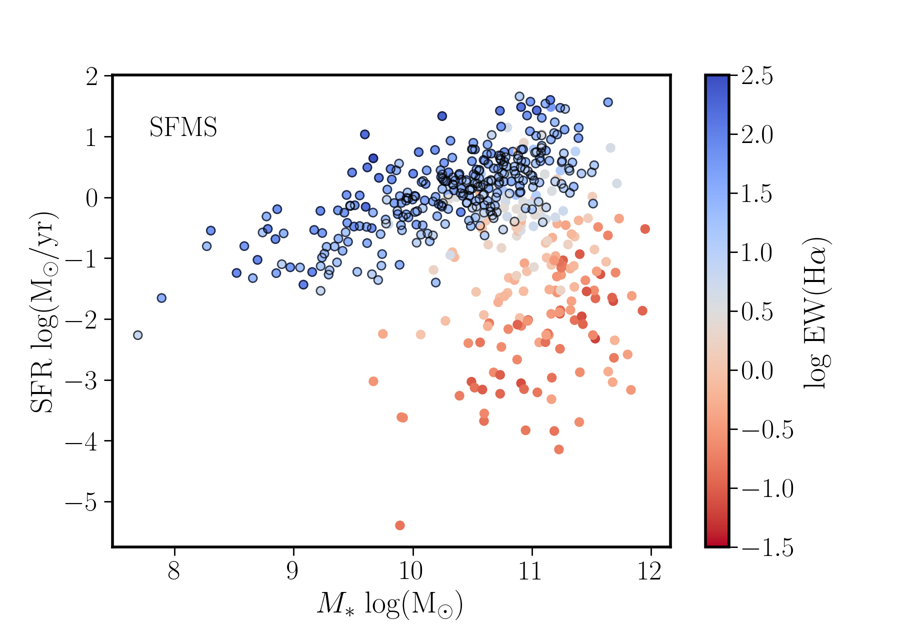
Figure 1: Distribution of the SFR along M_∗ for AMUSING++ galaxy compilation. Each solid-circle corresponds to one particular galaxy, color-coded by the EW(H$\alpha$) at the effective radius. Black open-circles indicate that SFGs selected from the original sample.

2 Sample and Data

We made use of the data provided by AMUSING++ compilation (López-Cobá et al., 2020), a set of observations using MUSE on galaxies in the nearby Universe ($z\sim$0.03), that comprises $\sim$600 galaxies (in the current compilation). These observations comprises the galaxies included in the AMUSING survey (PI: J. Anderson), and data retrieved from the ESO archive. All galaxies were selected to match their optical extension with the FoV of the MUSE instrument ($\sim$1 arcmin²), in a way that it covers between 1.0 and 2.0 effective radius. We exclude edge-on galaxies, i.e., with inclination larger than 70^o, to avoid possible issues related with highly inclined galaxies. All data were analyzed using the Pipe3D pipeline (Sánchez et al., 2016; Lacerda et al., 2022), a tool aimed to separate the stellar population and emission line properties of the galaxies. Using this tool we retrieve for each galaxy: (i) the integrated stellar mass, M_∗, derived from via the decomposition of the stellar population spectra in a set of single-stellar populations spectra, which allows to estimate the average mass-to-light ratio; (ii) the integrated the star-formation rate, estimated using the dust-corrected H$\alpha$ luminosity, adopting the calibrator proposed by Kennicutt (1998a); and finally (iii) an estimation of the molecular gas mass (M_gas) based on the dust attenuation, using a modification of the calibrator proposed by Barrera-Ballesteros et al. (2020). All those quantities were derived using the procedures described in detail in Sánchez et al. (2021b) and Sánchez et al. (2022). In addition we retrieve the [OIII]/H$\beta$, [NII]/H$\alpha$ line ratios and the EW(H$\alpha$) measured at the effective radius. Using those data we define a sample of star-forming galaxies (SFGs) following Sánchez (2020), i.e., galaxies that are located below the Kewley et al. (2001) demarcation line in the BPT (Baldwin et al., 1981) diagram with an EW(H$\alpha$)$>$6Å. Figure 1 shows the distribution along the SFR-M_∗ plane of the 485 (non highly inclined) galaxies selected from the AMUSING++ compilation, together with the SFGs sub-sample, that comprises 297 galaxies. It is clearly seen that this compilation comprises galaxies of any star-formation stage, covering a wide range of stellar masses, and presumely a wide range of galaxy morphologies (as shown in López-Cobá et al., 2020). Finally, it is clear that our selected sub-sample of SFGs follow the expected trend along this diagram, i.e., the SFMS.

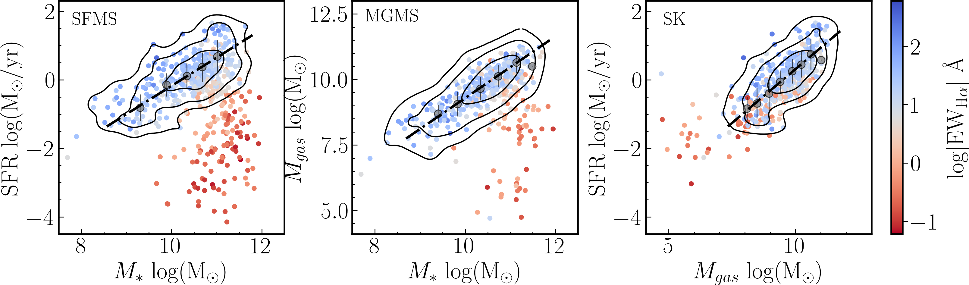
Figure 2: Distribution of the global extensive parameters: (i) SFR as a function of M_∗ (left panel), (ii) M_gas as a function of M_∗ (central panel) and (ii) SFR as a function of M_gas (right panel). In each panel each solid-circle corresponds to one AMUSING++ galaxy, color-coded by the EW(H$\alpha$) at the effective radius. The contours trace the density distribution of the SFGs (encircling 95%, 80% and 40% of this subsample, respectively). Grey solid-circles corresponds to the average values in bins of 0.2 dex in the x-axis, with the errorbars tracing the 1$\sigma$ distribution. Finally the dashed-lines correspond the best fitted relations: SFMS, MGMS and SK, in each case.

3 Analysis and Results

Following Cano-Díaz et al. (2019) we first explore the global extensive relations between the three retrieved parameters (SFR, M_∗ and M_gas), analyzing the distribution and relation between the SFR-M_∗ (SFMS), M_gas-M_∗ (MGMS) and SFR-M_gas (SK). Figure 2 show such distributions for the full sample of galaxies, highlighting the location of SFGs. As expected, in the three cases it is observed clear linear trends that define the well known relations. To parametrize them we perform a binning of the data in the x-axis, deriving the average and standard deviation in bins of 0.2 dex. The location of the binned data is shown in the different panels too. Then, we perform a simple linear regression for the binned data to derive the best fitted relation between both pairs of parameters. Equations 3.1, 3.2, and 3.3 show the results of this analysis. Errors were derived by performing a simple Monte-Carlo iteration on the original data, propagating the errors of each derived parameter.

$$log(SFR)=(0.83\pm 0.22)log(M_{*})-(8.43\mp 0.93)$$ (1)

$$log(M_{*})=(1.18\pm 0.21)log(M_{gas})-(2.52\mp 0.83)$$ (2)

$$log(SFR)=(0.63\pm 0.19)log(M_{gas})-(5.97\mp 0.67)$$ (3)

As expected we found three clear tight correlations between the analyzed extensive parameters. In all cases the slopes are near one, or slightly lower, by compatible within $\sim$2$\sigma$ with this value. The largest deviation from this value is reported for the SK-law, most probably due to the more limited dynamical range of the two parameters involved in this relation.

Once derived the extensive relations, we repeat the analysis using the global intensive relations ($\Sigma_{\rm SFR}$ , $\Sigma_{\rm*}$ and $\Sigma_{\rm mol}$ ). To derive those parameters we follow Sánchez et al. (2021b), dividing the corresponding extensive parameter by the effective area covered by each galaxy (defined as 4$\pi$R${}^{2}_{e}$, i.e., the area encircled in 2 effective radius). Figure 3 show the distribution of parameters and the results of the binning and fitting analysis, with the best fitted linear relations listed in Equations 3.4, 3.5, and 3.6.

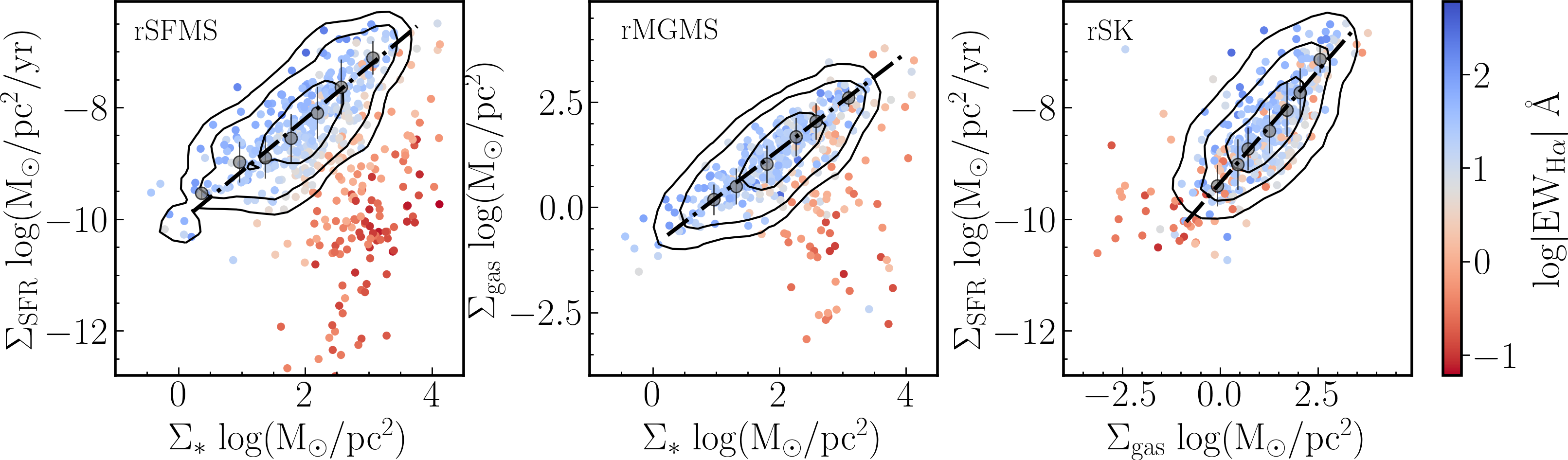
Figure 3: Distribution of the global intensive parameters: (i) $\Sigma_{\rm SFR}$ as a function of $\Sigma_{\star}$ (left panel), (ii) $\Sigma_{\rm gas}$ as a function of $\Sigma_{\star}$ (central panel) and (ii) $\Sigma_{\rm SFR}$ as a function of $\Sigma_{\rm gas}$ (right panel). In each panel each solid-circle corresponds to one AMUSING++ galaxy, color-coded by the EW(H$\alpha$) at the effective radius. The contours trace the density distribution of the SFGs (encircling 95%, 80% and 40% of this subsample, respectively). Grey solid-circles corresponds to the average values in bins of 0.2 dex in the x-axis, with the errorbars tracing the 1$\sigma$ distribution. Finally the dashed-lines correspond the best fitted global intensive relations relations: rSFMS, rMGMS and rSK, in each case.

$$log({\Sigma}_{SFR})=(0.94\pm 0.22)log({\Sigma}_{*})-(10.08\mp 0.35)$$ (4)

$$log({\Sigma}_{gas})=(1.15\pm 0.19)log({\Sigma}_{*})-(0.92\mp 0.30)$$ (5)

$$log({\Sigma}_{SFR})=(0.80\pm 0.18)log({\Sigma}_{gas})-(9.34\mp 0.22)$$ (6)

As expected the three distributions show a clear tight relation between the involved pair of parameters, correlations that a tighter than the extensive ones, with a lower error for both the slopes and zero-points. Furthermore, the slopes are in all cases more near to one, within less than 1$\sigma$ in the case of the rSFMS and rMGMS relations and just at 1$\sigma$ for the rSK one.

Table 1: Results of the analysis of global intensive relations rSFMS, rSK y rMGMS

References	$\beta$	$\alpha$	rc	$\sigma_{\rm obs}$	$\sigma_{exp}$	#	#
						Gal.	SFG
rSFMS
AMUSING++	-10.08$\pm$0.35	0.94$\pm$0.22	0.79	0.466	0.290	485	297
Sa21a(EDGE)	-10.10$\pm$0.22	1.02$\pm$0.16	0.68	0.266	0.190	126	12667
Sa21a(CALIFA)	-10.27$\pm$0.22	1.01$\pm$0.15	0.85	0.244	0.192	941	533
Sa21a(APEX)	-9.78$\pm$0.30	0.74$\pm$0.21	0.76	0.226	0.211	512	251
Wu13	-8.41	0.95
CD16	-10.19$\pm$0.33	0.72$\pm$0.04	0.63	0.16
Li19	-10.54$\pm$0.11	1.19$\pm$0.01		0.25		14	5383∗
CD19	-10.48$\pm$0.69	0.94$\pm$0.08	0.62	0.27		2737	$\sim$500K
Sa21	-10.35$\pm$0.03	0.98$\pm$0.02	0.96	0.17		1512	$\sim$3M
El20	-10.07$\pm$1.44	1.03$\pm$0.17	0.57	0.28-0.39		28	$\sim$15035∗
rSK
AMUSING++	-9.34$\pm$0.22	0.80$\pm$0.18	0.8	0.478	0.294	485	297
Sa21a(EDGE)	-9.01$\pm$0.14	0.98$\pm$0.14	0.73	0.249	0.216	126	12667
Sa21a(CALIFA)	-9.01$\pm$0.16	0.95$\pm$0.21	0.77	0.293	0.297	941	533
Sa21a(APEX)	-8.84$\pm$0.24	0.76$\pm$0.27	0.70	0.294	0.228	512	351
Bo17	-9.22	1.00				104	$\sim$5000
Li19	-9.03$\pm$0.06	1.05$\pm$0.01		0.19		14	5383∗
El20	-8.87$\pm$0.66	1.05$\pm$0.19	0.74	0.22-0.32		28	$\sim$15035∗
rMGMS
AMUSING++	-0.92$\pm$0.30	1.15$\pm$0.19	0.85	0.528	0.283	485	297
Sa21a(EDGE)	-0.91$\pm$0.16	0.93$\pm$0.11	0.68	0.218	0.209	126	12667
Sa21a(CALIFA)	-1.12$\pm$0.27	0.93$\pm$0.18	0.74	0.276	0.288	941	533
Sa21a(APEX)	-0.70$\pm$0.37	0.73$\pm$0.24	0.73	0.234	0.212	512	251
Li19	-0.59$\pm$0.08	1.10$\pm$0.01		0.20		14	5383∗
BB20	-0.95	0.93		0.20		93	$\sim$5000
El20	-0.99$\pm$0.13	0.88$\pm$0.15	0.72	0.21-0.28		28	$\sim$15035∗

Table 2: Zero-point ($\beta$) and slope ($\alpha$) of the three intensive global relations explored along this study (rSFMS, rSK and rMGMS), together with the values reported for a selection of similar relations extracted from the literature: Sánchez et al. (2021c)(Sa21a), Wuyts et al. (2013)(Wu13), Cano-Díaz et al. (2016b)(CD16), Lin et al. (2019)(Li19), Cano-Díaz et al. (2019)(CD19), Sánchez et al. (2021b)(Sa21) y Ellison et al. (2020a)(El20), Sánchez et al. (2021b)(Sa21), Bolatto et al. (2017)(Bo17), Lin et al. (2019)(Li19) and Barrera-Ballesteros et al. (2020)(BB20) y Ellison et al. (2020a)(El20). In addition we include the correlation coefficient ($r_{c}$), the standard deviation of the distribution of data before ($\sigma_{\rm obs}$) and after applying the best fitted linear relation ($\sigma_{\rm exp}$), together with the number of galaxies or number of individual spatial elements considered in the analysis. In italics we highlight the results from spatially resolved data, and in non-italics are indicated the explorations based on global intensive parameters.

4 Conclusions

Table 2 present a summary of the results together with similar values reported in the literature for both global intensive relations (Fig. 3), and local/resolved ones. From this comparison it is seen that:

• Global intensive parameters present a niche of opportunity to explore the physics of star-formation in a more coherent way than extensive ones, providing tighter and better defined relations (as the galaxy extension and aperture effects are limited).

• Global intensive relations can be directly compared with local/resolved ones (at least down to 1 kpc), showing similar trends both qualitatively and quantitatively, suggesting that they are originated by the same physical processes.

• There are hints of the evolution of the local/resolved relations that are evident when comparing results from sample at different redshits (e.g. Wuyts et al. (2013) vs. the rest of the data)

• If there is any secondary relation or a hierarchy among the relations, it is required to explore them on the tighter and best defined set of data.

In this regards, we need to highlight that it is still an open question which is of the explored relations is more fundamental than the previous one (if any). The nature of the scatter described in the three relations and the existence of possible secondary relations with other parameters, that may drive this scatter, is indeed and important topic of study. As indicated before, it could be the case that these relations depends on the morphology, that may affect the star-formation efficiency (SFE). Some authors have reported that the rSFMS preent a secondary relation that depends on the SFE (Ellison et al., 2020b, using the ALMAQUEST data) or the gas fraction (Colombo et al., 2020). This has open the seek for a more fundamental relation that involves pairs of parameters to trace the SFR (e.g. Shi et al., 2018; Dey et al., 2019; Barrera-Ballesteros et al., 2021). However, other results indicate that most probably those secondary relations are pure mathematical artifact introduced by correlation between errors (Sánchez et al., 2021c). The use of a larger samples, the tighter and better defined relations (i.e., the intensive ones), and better methods to derive the parameters (in particular for the molecular gas), seem to be required approach to perform future explorations.