Specifying Behavior Preference with Tiered Reward Functions

Abstract

Reinforcement-learning agents seek to maximize a reward signal through environmental interactions. As humans, our contribution to the learning process is through designing the reward function. Like programmers, we have a behavior in mind and have to translate it into a formal specification, namely rewards. In this work, we consider the reward-design problem in tasks formulated as reaching desirable states and avoiding undesirable states. To start, we propose a strict partial ordering of the policy space. We prefer policies that reach the good states faster and with higher probability while avoiding the bad states longer. Next, we propose an environment-independent tiered reward structure and show it is guaranteed to induce policies that are Pareto-optimal according to our preference relation. Finally, we empirically evaluate tiered reward functions on several environments and show they induce desired behavior and lead to fast learning.

1 Introduction

Reinforcement learning (Sutton and Barto 1998) is concerned with the problem of learning to behave to maximize a reward signal. In biological systems, this reward signal is considered to be the organism’s motivational system, using pain and pleasure to modulate behavior. In engineered systems, however, rewards must be selected by the system designer. We view rewards as a kind of programming language—a specification of the agent’s target behavior (Littman et al. 2017). As arbiters of correctness in the learning process, humans bear the responsibility of authoring this program.

There are two essential steps in designing reward functions. First, one must decide what kind of behavior is desirable and should be conveyed. Then, there’s the choice of reward function that induces such behavior.

In this paper, we look at a specification language that allows for the expression of desirable states (goals and subgoals) and undesirable states (obstacles). Even in this simple setting, providing precise trade-offs is difficult. Is it better for an agent to increase the chance of getting to the goal by 5% if it also incurs 8% higher probability of hitting an obstacle? Is it better to increase by 50% the probability of getting to a goal if the expected time of getting there also increases by 20%? There is no universal preference over behavior and having to explicitly write down all possible trade-offs is challenging. Even if the reward designer has a way of expressing preferences for all possible exchanges, it can be difficult, impossible even, to design a reward function that captures them without prior knowledge of the environment.

Our contribution is twofold: First, we define a preference over the entire policy space via a strict partial ordering on outcomes. Then, we introduce a class of environment-independent tiered reward functions that provably induce Pareto-optimal policies with respect to this preference ordering, empirically showing they lead to fast learning.

Favorable Policies

In the goal–obstacle class of tasks we consider, preferences over policies are simplest in the deterministic setting. We imagine all states are either goal states, obstacle states, or neither (background states). All goal states and obstacle states are absorbing. A policy from a fixed known (background) start state will either first reach a goal in $g$ steps, first reach an obstacle in $o$ steps, or run forever remaining in background states without reaching either. We prefer a policy that reaches a goal in $g_{1}$ steps to one that reaches a goal in $g_{2}$ steps if $g_{1}<g_{2}$. (Reaching a goal faster is better.) We prefer a policy that reaches a goal to one that does not. We prefer a policy that reaches neither a goal nor obstacle to one that reaches an obstacle. And we prefer a policy that reaches an obstacle in $o_{1}$ steps to one that reaches an obstacle in $o_{2}$ steps if $o_{1}>o_{2}$. (Taking longer to encounter an obstacle is better.) Two different policies that both reach a goal or both reach an obstacle and take the same number of steps to do so are considered equally good. (Steps are indistinguishable.) Thus, in deterministic domains, these preferences form a total order.

As pointed out before, preferences are less clear in a stochastic setting because there can be trade-offs between different outcomes and their probabilities. However, some comparisons are arguably clear cut. Informally, if one policy induces uniformly better outcomes than another—being more likely to reach a goal and doing so faster, being less likely to reach an obstacle and getting there more slowly—we prefer such a policy. If the policies can’t be directly compared, we propose to be indifferent between them. Thus, we replace the standard reinforcement-learning notion of optimality with Pareto-optimality (Mornati 2013)—seeking a policy that is either preferred or incomparable to every other policy. Pareto-optimal policies are commonly adopted in the subfield of multiobjective RL (Vamplew et al. 2011).

Reward Design

Policies in general are hard to express through reward functions (Amodei and Clark 2016), and some are even impossible to convey with a Markov (state–action-based) reward (Abel et al. 2021). Even when policies are expressible, designing bad reward functions can lead to undesirable or dangerous actions (Amodei and Clark 2016), easy reward hacking (Amodei et al. 2016), and more. We seek to design good reward functions, which can be characterized by many properties, such as interpretability and learning speed (Devidze et al. 2021). But the most important property a reward function must have is to guarantee the adoption of a desired policy. As we will show later in Section 5, even some intuitively correct reward designs can lead to suboptimal policies. To hedge against this concern, we introduce a tiered reward structure that is guaranteed to induce Pareto-optimal policies. Intuitively, we partition the state space into several tiers, or goodness levels. States in the same tier are associated with the same reward, while states in a more desirable tier are associated with a proportionally higher reward. We prove that these tiered reward structures, with the proper constraints between reward values, induce Pareto-optimal behavior and empirically show that they can lead to fast learning.

2 Related Work

There are many papers that deal with specifying behavior through rewards. Reward machines (Icarte et al. 2022) allow different rewards to be delivered given differences in the agent’s trajectory. Our focus on how to provide incentives for specific outcomes is complementary and the two approaches can be used in concert. Temporal logic based languages (Littman et al. 2017; Camacho et al. 2019) have been used to specify behavior. Though these methods can be more expressive, they often lead to intractable planning and learning problems and we offer a different expressibility–tractability tradeoff. Preference-based RL methods (Brown et al. 2019) learn a reward function based on a dataset of preferences over trajectories. But, as we have shown, preferences can be very difficult to express. Our reward scheme relieves the need for environment-specific datasets created by human experts. Multi-objective RL (Vamplew et al. 2011) allows for different tasks to be specified through a set of reward functions. Our work proceeds in the orthogonal direction by designing a single reward function to trade off among multiple behaviors.

3 Background

First, we will establish the problem setting. We view a reinforcement-learning environment as a Markov Decision Process (MDP), with state space $S$, action space $A$, transition model $T$, reward function $R$, and discount factor $\gamma$. A policy $\pi:S\times A\rightarrow[0,1]$ is a mapping from the current state to a probability distribution of the action to be taken. The optimal policy starting from some initial state $s_{0}$ in the MDP is defined as any reward-maximizing policy $\pi^{*}\in\operatorname*{argmax}_{\pi}\mathbb{E}[\sum_{t}\gamma^{t}r_{t}|s_{0},\pi]$. To make the reward-design problem as simple as possible for designers, we limit the reward function $R:S\rightarrow\mathbb{R}$ to be defined solely on states. In goal–obstacle tasks, the goal states and obstacle states are absorbing.

We imagine the state space $S$ as exhibiting a tiered structure, where higher tiers are more desirable than lower tiers, and states within the same tier are equally desirable. We formally define a Tier MDP as:

Definition 1.

$k$-Tier Markov Decision Process: A Tier MDP is an MDP with state space $S$, action space $A$, transition model $T:S\times A\times S\rightarrow\mathbb{R}$, reward function $R:S\rightarrow\mathbb{R}$, and discount factor $\gamma$. The state space is partitioned into $k$ tiers, where $S=S_{1}\mathbin{\mathaccent 0{\cdot}\cup}S_{2}\mathbin{\mathaccent 0{\cdot}\cup}\ldots\mathbin{\mathaccent 0{\cdot}\cup}S_{k}$ and $S_{i}\cap S_{j}=\emptyset,\forall i\neq j\in 1,2,...,k$. The reward function has the form $R(s)=r_{i},\forall s\in S_{i},i=1,2,...,k$. In addition, $r_{1}<r_{2}<\ldots<r_{k}$.

As an example, the grid world from Russell and Norvig (2010), as illustrated in Figure 1, could be formulated as a 3-Tier MDP—the goal state is one tier ($S_{3}$), the lava state one tier ($S_{1}$), and all other states reside in the background tier ($S_{2}$). It is important to note that we put no constraints on how many states could be in each tier, nor how many tiers there can be. Therefore, the framework has a high degree of generality; any finite MDP with reward defined on states could be formulated as a Tier MDP by placing states with the same reward in the same tier. However, the Tier MDP is most useful when there are clear good and bad states in the state space, such as when there are goal and obstacle states, or even states of intermediate desirability such as subgoal states. In the following sections, we will show how to perform reward design in Tier MDPs.

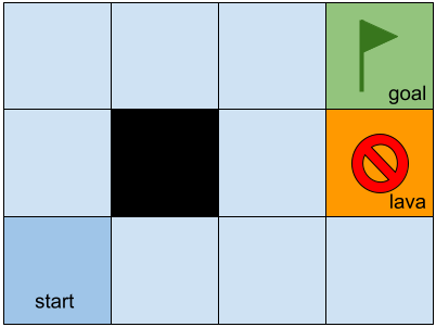
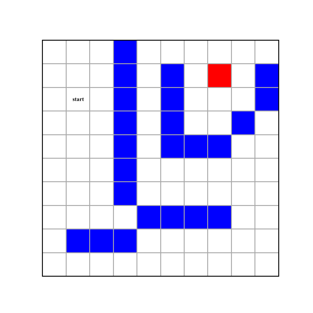
Figure 1: Left: Russell/Norvig grid world. Objective is to reach the goal (green) without first visiting lava (red) ($\gamma=0.9$). Right: A puddle world. Objective is to reach the goal (red) without crossing any puddles (blue) ($\gamma=0.99$). For both environments, the agent has probability $0.8$ of moving to the specified direction at each step, and probability $0.1$ of slipping to either side.

4 Policy Ordering

A policy can be thought of as inducing a probability distribution over an infinite set of outcomes (specifically the probability of reaching each of the states after $t$ steps, for all $t$). In goal–obstacle tasks, policies can be characterized by statistics such as probability of reaching the goal and probability of avoiding the obstacle for each possible horizon length.

For the moment, we will limit the problem space to 3-Tier MDPs for simplicity, and generalize to $k$-Tier MDPs in Section 6. In a 3-Tier MDP, we will call the 3 tiers obstacles ($S_{1}$), background ($S_{2}$), and goals ($S_{3}$), in order of increasing desirability. States in $S_{1}$ and $S_{3}$ are absorbing. We define $o_{t}$ to be the probability of being in $S_{1}$ at timestep $t$, and $g_{t}$ that of $S_{3}$.

Given two policies $\pi^{A}$ and $\pi^{B}$, we say $\pi^{A}$ dominates $\pi^{B}$ when both of these inequalities hold (and not both being strictly equal at all times):

$$\sum_{i=0}^{t}o_{i}^{A}\leq\sum_{i=0}^{t}o_{i}^{B},\quad\forall t=0,1,2,...,\infty,$$

$$\sum_{i=0}^{t}g_{i}^{A}\geq\sum_{i=0}^{t}g_{i}^{B},\quad\forall t=0,1,2,...,\infty.$$

In words, one policy dominates another if it gets to the goal faster, while delaying encountering obstacles longer. The set of policies that are not dominated by any other policy is the set of Pareto-optimal policies. Because there is a finite number of policies and domination is transitive, the set of Pareto-optimal policies is non-empty.

Going back to the example of the Russell/Norvig grid, we can visualize how the probability of reaching the goal ($g_{t}$) and reaching lava ($o_{t}$) changes over time for different policies. Consider two simple policies on the Russell/Norvig grid—(1) going left from all states (“always left”) and (2) going right from all states (“always right”).

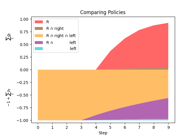
Figure 2: Visualization of the policies of always going left and always going right in the (stochastic) Russell/Norvig grid. The policy $R$ is the same as $R$ in Figure 3. To avoid color overlapping, we separated each policy into disjoint regions visualized by distinct colors. Each colored region in the figure represent the probability-region of one or more policies, joined by $\cap$. For example, the policy “always right” covers the areas in brown and orange.

We visualize each policy as a shaded area upper bounded by $\sum_{t}g_{t}$ and lower bounded by $-1+\sum_{t}o_{t}$ in Figure 2. This visualization can be understood as separating the probability space into two, with the goal-reaching probability on the top half of the y-axis in $[0,1]$ and obstacle-hitting probability in the bottom half of the y-axis in $[-1,0]$. With this visualization, a Pareto-dominated policy will cover an area that is entirely enclosed by that of a dominating policy because of lower goal-reaching probabilities on the top half and higher obstacle-hitting probabilities on the bottom half. As Figure 2 shows, “always right” and “always left” do not cover each other, so they are incomparable. Specifically, “always right” has a slightly higher probability of reaching the goal (brown), but “always left’ has a lower probability of reaching the lava (purple and teal).

For comparison, we plot another policy, which we call $R$, that is state-dependent and moves in the direction of the goal. For policy $R$, the probability of reaching the target increases with time because each step has a 20% slip probability; agents could slip early on and take longer to reach the goal. Note that area covered by $R$ (red, brown, orange, and purple) completely subsumes that of “always right” (brown and orange), demonstrating that “always right” is dominated by $R$. “Always left”, on the other hand, is not dominated by $R$ because it has a lower probability of reaching lava (teal). However, “always left” is not Pareto-optimal of course, because it is dominated by policy $G$ in Figure 3 (although this is not shown in the plot).

Pareto-optimal policies are interesting to consider for two main reasons. First, Pareto-optimal behavior always exists, even when policies that achieve other reasonable things do not. Take another 3-Tier MDP, the puddle world environment, for example. In this $10\times 10$ grid world, the objective is to reach the goal state without crossing any puddles (Figure 1 right). The goal state is absorbing while puddle and background states are not. Each step has probability $p$ of succeeding, and probability $\frac{1-p}{2}$ of slipping to either sides. However, when $p<0.87$, there is no state–based reward function that can encourage the agent to circle around on dry land to get to the goal (Littman 2015). Instead, the agent will either cower in the left corner (e.g., with $-1$ each step, $-70$ for puddle, and $+0$ at goal), cross over the first puddle strip and pass through the dry land on top (e.g., with $-1$ each step, $-35$ for puddle, and $+0$ at goal), or completely ignore the existence of puddles and get to the goal as directly as possible (e.g., with $-1$ each step, $-0$ for puddle, and $+0$ at goal). Even though there are no rewards to express this target objective, Pareto-optimal policies still exist and can be expressed.

Secondly, Pareto-optimality resolves the preference problem by defining a strict partial ordering over the entire policy space. Although the policies on the Pareto frontier are incomparable among themselves, they are all better than the set of Pareto-dominated policies. We simply deem the set of Pareto-optimal policies the desirable behavior, and all others undesirable. Next, we show how to design rewards that guarantee reward–optimal policies are selected from this set.

5 Tiered Reward

In this section, we seek a sufficient condition on the reward function so that optimizing expected discounted reward will always result in a Pareto-optimal policy with respect to our preference relation.

Definition 2.

Pareto-optimal rewards: A reward function $R(s)$ is called Pareto-optimal if the policy it induces, $\pi_{R}\in\operatorname*{argmax}_{\pi}\mathbb{E}[\sum_{t}\gamma^{t}r_{t}|s_{0},\pi]$, is Pareto-optimal.

Even some reasonable-sounding reward functions need not be Pareto-optimal. Going back to the Russell/Norvig grid example, an intuitive reward design would be requiring $r_{lava}<r_{back}<r_{goal}$. Consider three example reward functions that satisfy this constraint:

Policy	$r_{lava}$	$r_{back}$	$r_{goal}$
R	$-1$	$-0.1$	$+1$
G	$-1$	$0$	$+0.5$
B	$-1$	$-0.9$	$0$

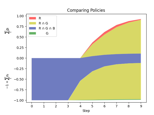
Figure 3: Visualization of three different policies (R, G, B) on Russell/Norvig grid. Visualization scheme is the same as described in Figure 2.

Both $R$ and $G$ are Pareto-optimal, while $B$ is Pareto-dominated (see Figure 3, where $B$’s areas are entirely enclosed by that of $R$ and of $G$). Roughly, $B$ doesn’t encourage getting to the goal but is also not particularly good at avoiding lava.

In fact, many of the reward functions that satisfy $r_{lava}<r_{back}<r_{goal}$ are not Pareto-optimal. Out of 1000 such rewards that we sampled randomly, 90.5% were Pareto-dominated. Next, we present a simple rule that is sufficient to guarantee environment-independent Pareto-optimal reward functions in 3-Tier MDPs.

Definition 3.

Tiered Reward: In a $3$-Tier Markov Decision Process with discount factor $\gamma\in(0,1)$, a reward function defined by

$$R(s)=\begin{cases}r_{obs}&\text{if\ }s\in S_{1}\\ r_{back}&\text{if\ }s\in S_{2}\\ r_{goal}&\text{if\ }s\in S_{3}\\ \end{cases}$$

is considered a Tiered Reward if

$$r_{obs}<\frac{1}{1-\gamma}r_{back}<r_{goal}.$$

and states in $S_{1}$ and $S_{3}$ are absorbing.

Theorem 1 (Pareto-optimal rewards in 3-Tier MDP).

In a 3-Tier Markov Decision Process, a Tiered Reward is Pareto-optimal.

Proof.

Let $\pi^{*}$ be the optimal policy induced with Tiered Reward $R(s)$. Suppose, for the sake of contradiction, there exists some policy $\pi$ that dominates $\pi^{*}$. Then, by our definition of Pareto dominance,

$$\sum_{i=0}^{t}o_{i}\leq\sum_{i=0}^{t}o_{i}^{*},\quad\forall t=0,1,2,...,\infty,$$

$$\sum_{i=0}^{t}g_{i}\geq\sum_{i=0}^{t}g_{i}^{*},\quad\forall t=0,1,2,...,\infty,$$

where $o_{t}$ and $g_{t}$ are the probabilities of reaching obstacles and goals in exactly $t$ steps following $\pi$, and $o_{t}^{*}$ and $g_{t}^{*}$ are the same for $\pi^{*}$. We can write the value function (of $\pi$ being evaluated on $R(s)$) as

$$V=\sum_{t=0}^{\infty}g_{t}(\gamma^{t}r_{goal}+\sum_{j=0}^{t-1}\gamma^{j}r_{back})+o_{t}(\gamma^{t}r_{obs}+\sum_{j=0}^{t-1}\gamma^{j}r_{back}).$$

The value of $\pi^{*}$ ($V^{*}$) can be written similarly. Denote

$$f_{t}^{g}=\gamma^{t}r_{goal}+\sum_{j=0}^{t-1}\gamma^{j}r_{back},\rm{\ and}$$

$$f_{t}^{o}=\gamma^{t}r_{obs}+\sum_{j=0}^{t-1}\gamma^{j}r_{back}.$$

That is, $f^{t}_{g}$ is the reward obtained on a trajectory that reaches a goal in $t$ steps and $f^{t}_{o}$ is the reward obtained on a trajectory that reaches an obstacle in $t$ steps. With $r_{obs}<\frac{1}{1-\gamma}r_{back}<r_{goal}$, $f_{t}^{g}$ is strictly decreasing and $f_{t}^{o}$ strictly increasing with respect to $t$ (Proof in Appendix A). Then,

$$\begin{split}V-V^{*}&=\sum_{t=0}^{\infty}(g_{t}-g_{t}^{*})f_{t}^{g}+\sum_{t=0}^{\infty}(o_{t}-o_{t}^{*})f_{t}^{o}\\ &=\sum_{t=0}^{\infty}(\sum_{j=0}^{t}g_{j}-g_{j}^{*})(f_{t}^{g}-f_{t+1}^{g})\\ &\quad+\sum_{t=0}^{\infty}(\sum_{j=0}^{t}o_{j}-o_{j}^{*})(f_{t}^{o}-f_{t+1}^{o})\\ &>0+0\\ &=0.\end{split}$$

An elaboration of the pass from the first equality to the second is detailed in Appendix A. We have shown, through the value function, that $\pi$ is strictly better than $\pi^{*}$ with respect to the reward function $R$. But $\pi^{*}$ was chosen to optimize $R$, so that’s a contradiction. Since no such $\pi$ can exist, that means $\pi^{*}$ is not dominated by any policy, and is therefore Pareto-optimal. ∎

The constraint for Tiered Reward in Definition 3 can be understood intuitively. The middle term $\frac{1}{1-\gamma}r_{back}$ is equal to the cumulative discounted return for infinitely getting a reward in the background tier ($(1+\gamma+\gamma^{2}+...)r_{back}$). So, in a gross simplification, as long as the reward at the goal is more appealing than infinitely wandering in background states, and the obstacle less appealing, the reward induces behavior that arrives at the goal early and avoids the obstacles. Following this simple constraint, we as reward designers can easily create Pareto-optimal reward functions without requiring knowledge of the transition probabilities in the environment.

6 Generalizing to $k$ Tiers

In Sections 4 and 5, we limited the discussion to $3$-Tier MDPs. But MDPs with more than $3$ tiers can usefully model important problems such as those with well-defined subgoal states. Specifically, each subgoal region could be its own tier, instead of being grouped into one big background tier. Even though these problems could still be solved as a $3$-Tier MDP, more knowledge about the environment could help design better reward functions and accelerate learning. So, in this section, we consider the reward-design problem in Tier MDPs with more than three tiers.

Definition 4.

Tiered Reward: In a $k$-Tier($k>3$) Markov Decision Process with discount factor $\gamma\in(0,1)$ where the goal tier ($k$) is absorbing, the reward function $R$ is a Tiered Reward if $R(s)=r_{i},\forall s\in S_{i},i=1,2,...,k$, for reward values $r_{1},r_{2},...,r_{k}\in\mathbb{R}$, that satisfy

$$r_{1}<(\frac{1}{1-\gamma})r_{2}<(\frac{1}{1-\gamma})^{2}r_{3}<\cdot\cdot\cdot<(\frac{1}{1-\gamma})^{k-1}r_{k}\leq 0.$$

Notice that the Tiered Reward in the $k$ tiers case uses a stricter condition than that of $3$ tiers. First, all reward values are non-positive. We enforce this constraint not only because of mathematical convenience (used later in Equation 1), but also because step-wise penalty has been proved to support faster learning (Koenig and Simmons 1993). Specifically, with a zero-initialized value function, step penalties create an incentive for the agent to try state–action pairs it has never experienced before, resulting in rapid exploration. Secondly, the reward values of higher tiers are exponentially greater than the lower ones. For adjacent tiers $i$ and $i+1$, The reward values always satisfy $r_{i}<\frac{1}{1-\gamma}r_{i+1}<0$. One such reward is visualized in Figure 4.

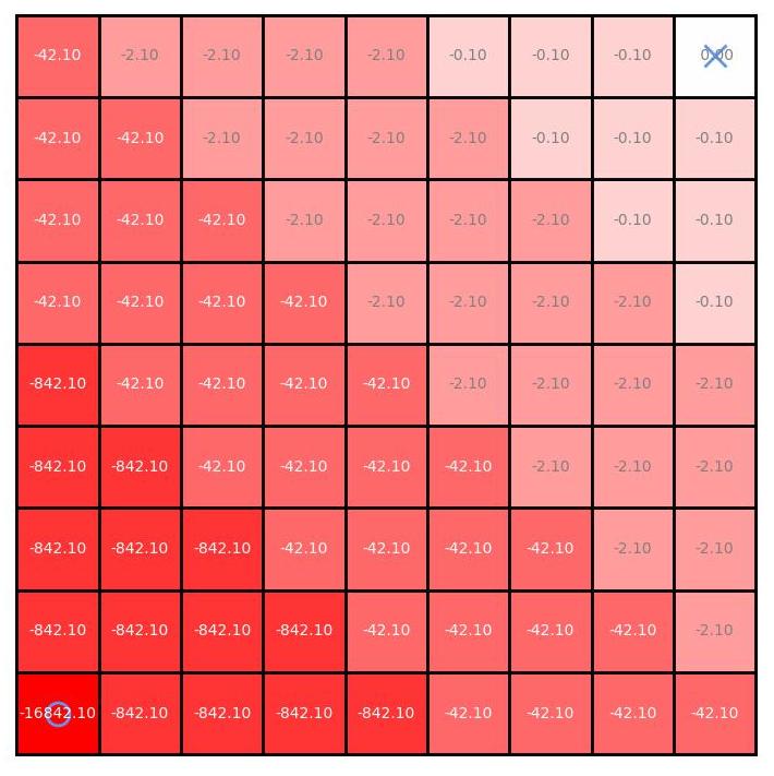
Figure 4: A Tiered Reward in a grid world with $6$ tiers. Start state is in the bottom left corner, goal state in top right.

This definition can be understood as a generalization of the 3-Tiered Reward. When the agent resides within tier $i\in\{2,3,...,k-2\}$, the $k$ tiers could be partitioned into $3$ groups to construct a 3-Tier MDP. In particular, $S_{1}$ will include tiers $1$ through $i-1$, $S_{2}$ is just tier $i$, and $S_{3}$ is tiers $i+1$ to $k$. Note that we can generalize Theorem 1 to allow states in $S_{1}$ and $S_{3}$ to have any reward values as long as they satisfy the inequality in Definition 3 for a fixed reward value in $S_{2}$. Namely, denote $r_{low}=\max\{r_{1},...,r_{i-1}\}$ and $r_{high}=\min\{r_{i+1},...,r_{k}\}$, and as a $k$-Tiered Reward they satisfy

$$r_{low}<(\frac{1}{1-\gamma})r_{i}<(\frac{1}{1-\gamma})^{2}r_{high}$$

And since $\gamma\in(0,1)$,

$$r_{low}<(\frac{1}{1-\gamma})r_{i}<(\frac{1}{1-\gamma})^{2}r_{high}\leq r_{high}.$$ (1)

That is, $(r_{low},r_{i},r_{high})$ is a Tiered Reward function in the $3$-Tier MDP with tiers $S_{1}$, $S_{2}$, and $S_{3}$, and therefore induces Pareto-optimal policies (Theorem 1). So, at tier $i$, the policy that optimizes the $k$-Tiered Reward will push agents to higher tiers as fast as possible and avoid lower tiers, as if they were goals and obstacles, respectively. In the special case that the agent resides within tier $i=1$, the constraint from Definition 4 will treat tiers $2$ through $k$ as if they are all goals, pushing the agent towards them. In the case that $i=k$, the agent is already in the “goal tier”. So overall, $k$-Tiered Reward will induce in a ratchet-like policy—go to the higher tiers as fast as possible while not fall back to the lower tiers—that makes learning fast. In fact, it has been shown that a similar increasing reward profile leads to fast learning (Sowerby, Zhou, and Littman 2022).

Besides encouraging early visitation of good tiers, using Tiered Reward also guarantees maximum total visitation of all good tiers. This property is formalized in Theorem 2.

Theorem 2 (Tiered Reward and Cumulative Tier Visitation).

In a $k$-Tier Markov Decision Process that has Tiered Reward $R(s)$, the induced optimal policy is $\pi^{*}$. Let ${p_{t}^{*}}^{d}\in[0,1]$ be the probability of being in tier $d\in\{1,2,...,k\}$ for the first time at timestep $t$ following policy $\pi^{*}$. Then, there is no policy $\pi$, along with its induced probability distribution $p_{t}^{d}$, that satisfies both:

$$\sum_{i=0}^{t}p_{i}^{1}\leq\sum_{i=0}^{t}{p_{i}^{*}}^{1},\quad\forall t=0,1,2,...,\infty,{\rm\ \it and}$$

$$\sum_{i=0}^{t}p_{i}^{d}\geq\sum_{i=0}^{t}{p_{i}^{*}}^{d},\quad\forall d=[2..k],\forall t=0,1,2,...,\infty.$$

The proof is similar to that of Theorem 1 and can be found in Appendix B. To state the theorem in words, if a $k$-Tier MDP has a Tiered Reward structure, then the resulting policy will visit the worst tier ($S_{1}$) for as few times as possible, while visiting all the other good tiers ($S_{2}$, …, $S_{k}$) as often as possible, respectively.

7 Experiments

In this section, we aim to verify the usefulness of our proposed Tiered Reward. We empirically show that the Tiered Rewards are able to make learning faster on multiple domains. We also explore the influence of the number of tiers and find that having more tiers can help induce faster learning.

The implementation of many environments and algorithms is based on the MSDM library by Ho, Correa, and Ritter (2021). All experiments are run on an Ubuntu $18.04$ system with an Intel Core i7-9700K CPU and $32$G of RAM.

Fast Learning with Tiered Rewards

Guaranteeing Pareto-optimal behavior is not the sole benefit of using Tiered Rewards; we find that it also leads to fast learning. There are many ways to design a Tiered Reward because it is a class of reward functions that is only constrained by an inequality (Definition 4), and not by specific reward values. In the following experiments, we use one instantiation of $k$-Tiered Reward:

$$r_{i}=\begin{cases}0&\text{if\ }i=k\\ \frac{1}{1-\gamma}r_{i+1}-\delta&\text{if \ }i<k\\ \end{cases}$$

where $\delta=0.1$ is used as a small constant to satisfy the strict inequality constraint.

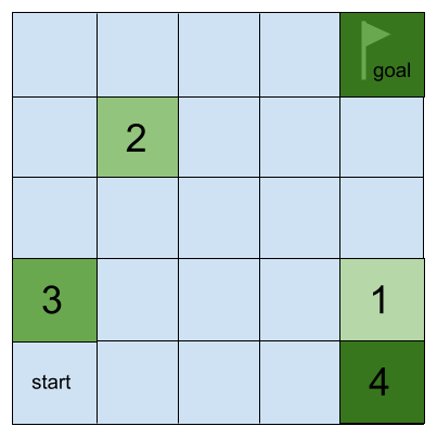
Figure 5: Flag grid by Ng, Harada, and Russell (1999)

.

The “Flag Grid” from Ng, Harada, and Russell (1999) is a natural $6$-Tier MDP to study Tiered Reward. In this grid world (Figure 5), the agent must learn to, starting at the bottom left corner, pick up $4$ flags in sequence, and finally go to the absorbing goal state. The state space is the location of the agent plus the flag it has collected. The agent can move in $4$ directions with an $80\%$ success rate, while acting randomly $20\%$ of the time. All states in which the agent possesses the same number of flags constitute a tier, totaling 5 tiers. The goal constitutes the 6th and final tier.

To evaluate Tiered Reward, we compare it against two baseline reward functions. The first one, following Koenig and Simmons (1993), we call action penalty. This reward penalizes each step with $-1$, until the goal state is reached and the agent is awarded $+1$. To reiterate, such negative step reinforcement encourages directed exploration. This reward only assumes knowledge about the position of the goal.

The Flag Grid domain was introduced in the context of potential-based shaping (Ng, Harada, and Russell 1999). In that work, the authors showed how knowledge of the subgoals could be leveraged through shaping rewards to guide the learning process. Our Tiered Rewards can be used similarly, so we compare potential-based shaping to Tiered Rewards in this environment. For direct comparability, we use the Tiered Reward as a potential function $\Phi(s)=R_{tier}(s)$ to shape the action-penalty reward, resulting in what we call tier-based shaping reward: $R_{tbs}(s,a,s^{\prime})=R_{penalty}(s)+\gamma\Phi(s^{\prime})-\Phi(s)$.

We compare these reward functions in the context of Q-Learning (Watkins and Dayan 1992), arguably the most well-understood and widely applicable RL algorithm. Following Koenig and Simmons (1993), we use a greedy policy for action selection and initialize the Q values optimistically to exploit directed exploration. Since all reward values are non-positive, it is sufficient to initialize the Q values to $0$. We use a learning rate of $\alpha=0.90$ (tuned from $\alpha\in\{0.95,0.90,0.85\}$, all of which performed similarly).

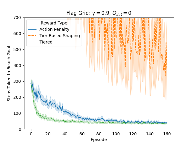
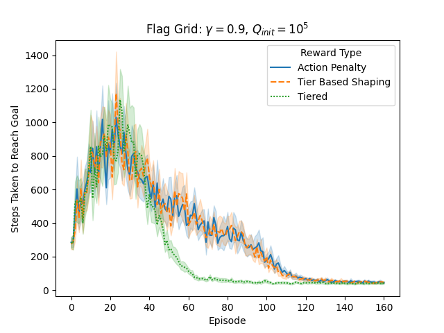
Figure 6: Q Learning curves for Flag Grid. The two plots use different initial Q values. Each experiment was run with $30$ seeds. We experimented with a range of discounts $\gamma\in\{0.99,0.95,0.90,0.85\}$ and found they all had similar performances, and only report $\gamma=0.90$ here.

As Figure 6 (left) shows, Tiered Reward always learns fastest of the three. Perhaps surprisingly, tier-based shaping reward performs orders of magnitudes worse than even action penalty. That is because, with discounting, the shaping function $F(s,a,s^{\prime})=\gamma\Phi(s^{\prime})-\Phi(s)$ becomes positive when $s$ and $s^{\prime}$ belong to the same tier. As a result, the zero-initialized Q values are not optimistic with respect to these rewards, and so exploration with $R_{tbs}$ is undirected, leading to slow learning. For a fairer comparison, we also plot the learning curves where all Q values are initialized to some arbitrary large value so that $R_{tbs}$ also enjoys directed exploration as the two other rewards (Figure 6 right). We tried different initialization values ($10^{10},10^{5},10^{3}$) and observed similar results, so we only report $Q_{init}=10^{5}$ here. There is a noticeable spike in time taken to reach the goal early on during training. It is the result of optimistic Q-value initialization, which leads to more exploration and thus slower learning. Regardless of this tradeoff, Tiered Reward still consistently outperforms the two baselines.

It is important to note that our goal here is not to argue shaping is ineffective, nor to determine how to initialize Q values for fast learning, but solely to demonstrate the usefulness of Tiered Reward in various different settings. To start, it makes learning faster than tier-based shaping reward and action penalty for different discount factors and Q value initialization schemes. Moreover, it is simple to design and implement; there is no need to engineer environment-specific reward and initial Q values to accelerate learning.

Influence of More Tiers

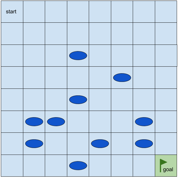
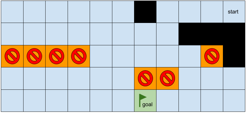
Figure 7: Left: Frozen lake environment with holes in dark blue. Right: Wall Grid environment with walls in black and lava in orange.

In Flag Grid, we kept the number of tiers to be a constant $6$ because of the structure of the environment. Here, we explore Tiered Reward with a varying number of tiers. Towards that goal, we choose for simplicity and clarity four grid-world domains that are suited to a flexible number of tiers:

1. Chain: a 90–state 1D environment with left and right actions. Starting from one end, the agent tries to reach the other end with actions of success rate $80\%$; failed actions transition to the opposite direction.

2. Grid: a $9\times 9$ grid where the agent starts in one corner and aims for the opposite corner. The agent can move in four cardinal directions with a $80\%$ success rate, while slipping to either side with a $10\%$ chance.

3. Frozen Lake: a slippery grid with holes that will swallow the agent (Figure 7 left). The objective is to get to the goal without falling into any holes. Each of the $4$ directional actions succeed $1/3$ of the time, and slip to either side with probability $1/3$.

4. Wall Grid: a grid world with multiple lava states and wall states (Figure 7 right). The agent has to circle around the walls while avoiding the lava to get to the goal. Transition dynamics same as Grid.

For Chain and Grid, tiers are decided based on their $L1$ distance to the goal; for Frozen Lake and Wall Grid, tiers are chosen based on the sum of $L1$ distance to the goal and start state, weighted $2:1$. Since there are $3$ different type of states in the latter two environments, we start at $3$ tiers instead of $2$. All goal and obstacle states are absorbing.

In each environment, we measure the learning speed by recording the steps required for the agent to reach the goal for the first time. For fair comparison, we optimistically initialize $Q_{init}=10^{5}$ so that $R_{tbs}$ also enjoys the benefit of directed exploration. The results are presented in Figure 8. As we expected, Tiered Reward makes learning faster as the number of tiers increases; more information about the environment aids reward design to accelerate learning. Tiered Reward consistently beats action penalty and is at least as good as tier-based shaping reward, and often much better. Even when Tiered Reward performs the same as shaped reward, it provides the added benefit of simplicity and better interpretability—it is based only on states, and not state–action–state triples.

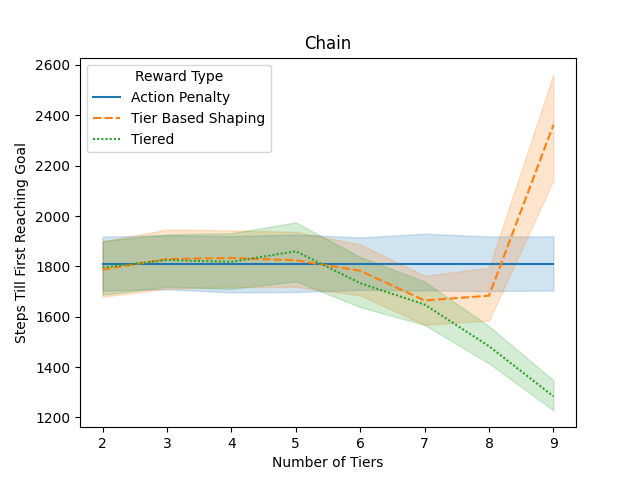
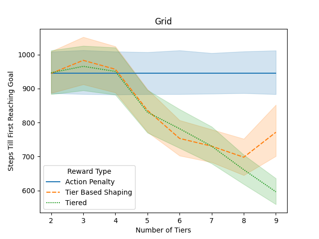
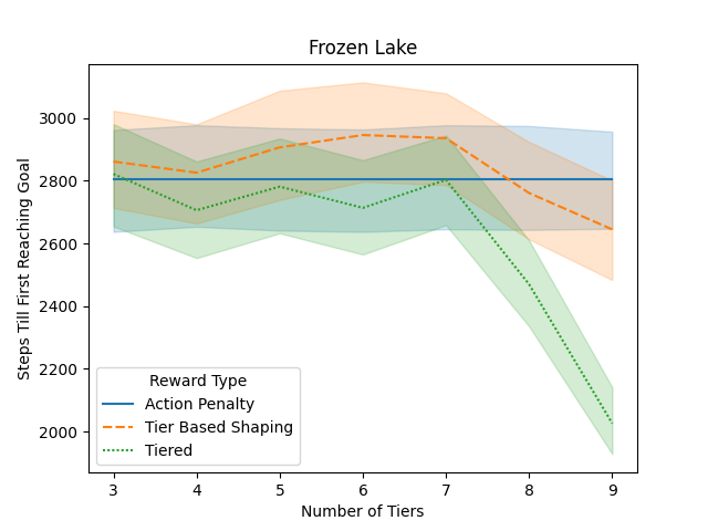
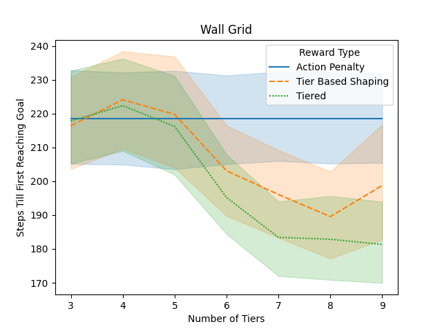
Figure 8: Q-Learning results with $\gamma=0.9$. Each experiment was run with $300$ seeds.

Finally, we show that Tiered Reward is not only environment-independent, but also learning algorithm agnostic. We repeat the same experiments with another learning algorithm, RMAX (Brafman and Tennenholtz 2002). We set maximal reward $r_{max}=10^{5}$ , use the first $m=3$ transition samples to model the MDP (tuned from $m\in\{2,3,5,7,10\}$ and selected based on good resulting policy while taking similar learning time to Q-Learning), and did $200$ iterations of value iteration during each update. The results are shown in Figure 9 and are similar to what was found with Q-Learning.

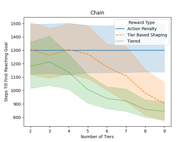
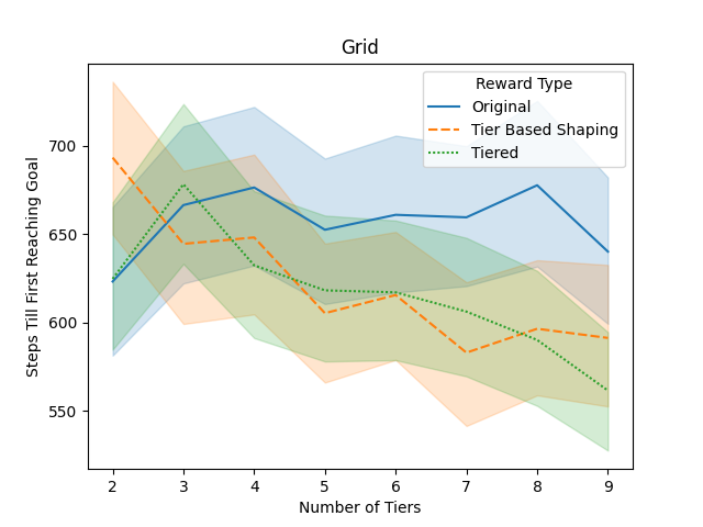
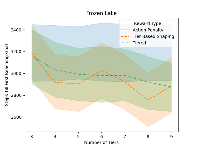
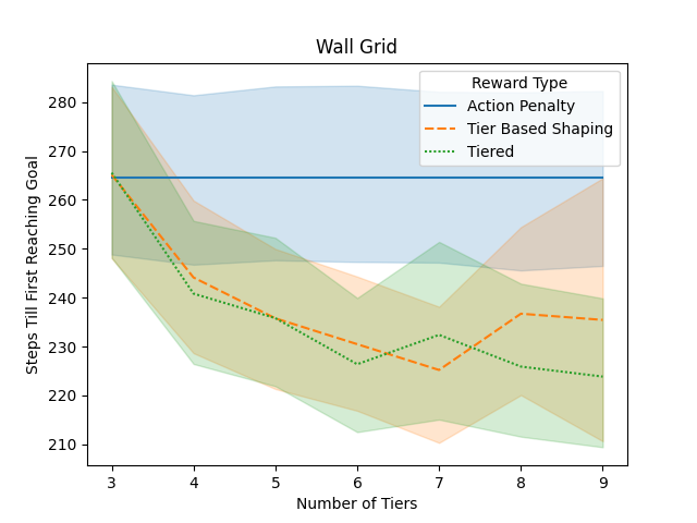
Figure 9: RMAX results with $\gamma=0.9$. Each experiment was run with $300$ seeds.

8 Conclusion

In contrast to standard reward-design solutions that are environment-dependent, we presented Tiered Rewards—a class of environment-independent reward functions that provably leads to (Pareto) optimal behavior and empirically leads to fast learning.

Future work includes theoretical guarantees that Tiered Reward lead to asymptotically faster learning and verifying the usefulness of Tiered Reward in scaled up Deep Reinforcement Learning domains.

Appendix A Details of Theorem 1 Proof

Proof that $f_{t}^{g}$ is strictly decreasing:

$$\begin{split}f_{t+1}^{g}-f_{t}^{g}&=\gamma^{t+1}r_{goal}+\sum_{j=0}^{t}\gamma^{j}r_{back}-\gamma^{t}r_{goal}-\sum_{j=0}^{t-1}\gamma^{j}r_{back}\\ &=\gamma^{t}(\gamma-1)r_{goal}+\gamma^{t}r_{back}\\ &=\gamma^{t}(1-\gamma)(\frac{1}{1-\gamma}r_{back}-r_{goal})\\ &<0\end{split}$$

because $0<\gamma<1$ and $\frac{1}{1-\gamma}<r_{goal}$.

Proof that $f_{t}^{o}$ is strictly increasing:

$$\begin{split}f_{t+1}^{o}-f_{t}^{o}&=\gamma^{t+1}r_{obs}+\sum_{j=0}^{t}\gamma^{j}r_{back}-\gamma^{t}r_{obs}-\sum_{j=0}^{t-1}\gamma^{j}r_{back}\\ &=\gamma^{t}(\gamma-1)r_{obs}+\gamma^{t}r_{back}\\ &=\gamma^{t}(1-\gamma)(\frac{1}{1-\gamma}r_{back}-r_{obs})\\ &>0\end{split}$$

because $0<\gamma<1$ and $r_{obs}<\frac{1}{1-\gamma}$.

An elaboration of the pass from the first equality to the second:

$$\begin{split}\sum_{t=0}^{\infty}(g_{t}-g_{t}^{*})f_{t}^{g}&=\sum_{t=0}^{\infty}\sum_{j=0}^{t}(g_{j}-g_{j}^{*})f_{t}^{g}-\sum_{t=0}^{\infty}\sum_{j=0}^{t-1}(g_{j}-g_{j}^{*})f_{t}^{g}\\ &=\sum_{t=0}^{\infty}\sum_{j=0}^{t}(g_{j}-g_{j}^{*})f_{t}^{g}-\sum_{t=1}^{\infty}\sum_{j=0}^{t-1}(g_{j}-g_{j}^{*})f_{t}^{g}\\ &=\sum_{t=0}^{\infty}\sum_{j=0}^{t}(g_{j}-g_{j}^{*})f_{t}^{g}-\sum_{t’=0}^{\infty}\sum_{j=0}^{t’}(g_{j}-g_{j}^{*})f_{t’+1}^{g}\\ &=\sum_{t=0}^{\infty}(\sum_{j=0}^{t}g_{j}-g_{j}^{*})(f_{t}^{g}-f_{t+1}^{g})\\ \end{split}$$

Similarly,

$$\sum_{t=0}^{\infty}(o_{t}-o_{t}^{*})f_{t}^{o}=\sum_{t=0}^{\infty}(\sum_{j=0}^{t}o_{j}-o_{j}^{*})(f_{t}^{o}-f_{t+1}^{o})$$

Appendix B Proof of Theorem 2

Proof.

The proof is similar to that of Theorem 1. Suppose, for the sake of contradiction, that there exists some such policy $\pi$. We can express the value functions as

$$V=\sum_{t=0}^{\infty}\gamma^{t}\sum_{m=1}^{k}r_{m}\cdot p_{t}^{m},{\rm\ and}$$

$$V^{*}=\sum_{t=0}^{\infty}\gamma^{t}\sum_{m=1}^{k}r_{m}\cdot{p_{t}^{*}}^{m}.$$

Denote $f_{t}^{m}=\gamma^{t}r_{m}$. Then, $f_{t}^{m}-f_{t+1}^{m}=r_{m}\gamma^{t}(1-\gamma)\leq 0,\forall m$. It’s easy to see $f_{t}^{m}-f_{t+1}^{m}$ is strictly increasing in $m$, so

$$\begin{split}V-V^{*}&=\sum_{t=0}^{\infty}\gamma^{t}\sum_{m=1}^{k}r_{m}(p_{t}^{m}-{p_{t}^{*}}^{m})\\ &=\sum_{m=1}^{k}\sum_{t=0}^{\infty}f_{t}^{m}(p_{t}^{m}-{p_{t}^{*}}^{m})\\ &=\sum_{m=1}^{k}\sum_{t=0}^{\infty}(f_{t}^{m}-f_{t+1}^{m})(\sum_{j=0}^{t}p_{j}^{m}-{p_{j}^{*}}^{m})\\ &>\sum_{m=1}^{k}\sum_{t=0}^{\infty}(f_{t}^{1}-f_{t+1}^{1})(\sum_{j=0}^{t}p_{j}^{m}-{p_{j}^{*}}^{m})\quad(*)\\ &=\sum_{t=0}^{\infty}(f_{t}^{1}-f_{t+1}^{1})\sum_{m=1}^{k}(\sum_{j=0}^{t}p_{j}^{m}-{p_{j}^{*}}^{m})\\ &=\sum_{t=0}^{\infty}(f_{t}^{1}-f_{t+1}^{1})\cdot\sum_{j=0}^{t}(\sum_{m=1}^{k}p_{j}^{m}-\sum_{m=1}^{k}{p_{j}^{*}}^{m})\\ &=\sum_{t=0}^{\infty}(f_{t}^{1}-f_{t+1}^{1})\cdot\sum_{j=0}^{t}(1-1)\\ &=0\end{split}$$

Note that the $(*)$ step is justified only because $\sum_{j=0}^{t}p_{j}^{m}-{p_{j}^{*}}^{m}\geq 0,\forall m=[2..k],\forall t$. The inequalities show that $\pi$ achieves higher reward than the optimal policy, which is a contradiction. No such $\pi$ exists. ∎

References

- Abel et al. (2021) Abel, D.; Dabney, W.; Harutyunyan, A.; Ho, M. K.; Littman, M.; Precup, D.; and Singh, S. 2021. On the expressivity of markov reward. Advances in Neural Information Processing Systems, 34: 7799–7812.
- Amodei and Clark (2016) Amodei, D.; and Clark, J. 2016. Faulty reward functions in the wild. URL: https://blog. openai. com/faulty-reward-functions.
- Amodei et al. (2016) Amodei, D.; Olah, C.; Steinhardt, J.; Christiano, P.; Schulman, J.; and Mané, D. 2016. Concrete problems in AI safety. arXiv preprint arXiv:1606.06565.
- Brafman and Tennenholtz (2002) Brafman, R. I.; and Tennenholtz, M. 2002. R-MAX—A General Polynomial Time Algorithm for Near-Optimal Reinforcement Learning. Journal of Machine Learning Research, 3: 213–231.
- Brown et al. (2019) Brown, D.; Goo, W.; Nagarajan, P.; and Niekum, S. 2019. Extrapolating beyond suboptimal demonstrations via inverse reinforcement learning from observations. In International conference on machine learning, 783–792. PMLR.
- Camacho et al. (2019) Camacho, A.; Icarte, R. T.; Klassen, T. Q.; Valenzano, R. A.; and McIlraith, S. A. 2019. LTL and Beyond: Formal Languages for Reward Function Specification in Reinforcement Learning. In IJCAI, volume 19, 6065–6073.
- Devidze et al. (2021) Devidze, R.; Radanovic, G.; Kamalaruban, P.; and Singla, A. 2021. Explicable reward design for reinforcement learning agents. Advances in Neural Information Processing Systems, 34: 20118–20131.
- Ho, Correa, and Ritter (2021) Ho, M. K.; Correa, C. G.; and Ritter, D. 2021. Models of Sequential Decision Making (msdm).
- Icarte et al. (2022) Icarte, R. T.; Klassen, T. Q.; Valenzano, R.; and McIlraith, S. A. 2022. Reward machines: Exploiting reward function structure in reinforcement learning. Journal of Artificial Intelligence Research, 73: 173–208.
- Koenig and Simmons (1993) Koenig, S.; and Simmons, R. G. 1993. Complexity analysis of real-time reinforcement learning. In AAAI, volume 93, 99–105.
- Littman (2015) Littman, M. L. 2015. Programming Agents via Rewards.
- Littman et al. (2017) Littman, M. L.; Topcu, U.; Fu, J.; Isbell, C.; Wen, M.; and MacGlashan, J. 2017. Environment-independent task specifications via GLTL. arXiv preprint arXiv:1704.04341.
- Mornati (2013) Mornati, F. 2013. Pareto Optimality in the work of Pareto. Revue européenne des sciences sociales. European Journal of Social Sciences, (51-2): 65–82.
- Ng, Harada, and Russell (1999) Ng, A. Y.; Harada, D.; and Russell, S. 1999. Policy invariance under reward transformations: Theory and application to reward shaping. In Icml, volume 99, 278–287.
- Russell and Norvig (2010) Russell, S. J.; and Norvig, P. 2010. Artificial Intelligence (A Modern Approach).
- Sowerby, Zhou, and Littman (2022) Sowerby, H.; Zhou, Z.; and Littman, M. L. 2022. Designing Rewards for Fast Learning.
- Sutton and Barto (1998) Sutton, R. S.; and Barto, A. G. 1998. Reinforcement Learning: An Introduction. The MIT Press.
- Vamplew et al. (2011) Vamplew, P.; Dazeley, R.; Berry, A.; Issabekov, R.; and Dekker, E. 2011. Empirical evaluation methods for multiobjective reinforcement learning algorithms. Machine Learning, 84(1): 51–80.
- Watkins and Dayan (1992) Watkins, C. J.; and Dayan, P. 1992. Q-learning. Machine learning, 8(3): 279–292.