Pseudo-Riemannian Embedding Models for Multi-Relational Graph Representations

Abstract

In this paper we generalize single-relation pseudo-Riemannian graph embedding models to multi-relational networks, and show that the typical approach of encoding relations as manifold transformations translates from the Riemannian to the pseudo-Riemannian case. In addition we construct a view of relations as separate spacetime submanifolds of multi-time manifolds, and consider an interpolation between a pseudo-Riemannian embedding model and its Wick-rotated Riemannian counterpart. We validate these extensions in the task of link prediction, focusing on flat Lorentzian manifolds, and demonstrate their use in both knowledge graph completion and knowledge discovery in a biological domain.

1 Introduction

A knowledge graph is a succinct abstraction of facts as a set of entities and their pairwise relations. Over the years, our ability to amass granular, heterogeneous relational data has increased substantially, allowing for graphical representations of entire systems, such as biology Himmelstein and Baranzini (2015) or society Bollacker et al. (2008). Learning expressive representations of these graphs is an important first step in many machine learning-enabled applications, from recommender systems to drug discovery.

One effective class of methods for learning these whole-graph representations is node embedding models Nickel et al. (2015). These models scale easily to large networks (Dettmers et al., 2018) and readily allow for applications such as node classification, clustering, and link prediction. The desire for low-dimensional yet expressive representations Seshadhri et al. (2020) of nodes in these complex networks has prompted the exploration of more general Riemannian manifold embeddings as an effective means of incorporating useful inductive biases (see for example Trouillon et al. (2016); Nickel and Kiela (2017); Gu et al. (2018); Suzuki et al. (2019); López et al. (2021)).

A more recent development is pseudo-Riemannian manifold embeddings for graph representations Sim et al. (2021). Unlike their Riemannian manifold counterparts, pseudo-Riemannian embeddings are free from a host of metric space constraints, such as the upper bound on the number of disconnected nearest neighbors of a given node Sun et al. (2015). As identified in Sim et al. (2021), there are many real-world examples, where these constraints are routinely violated, and where the introduction of an indefinite metric enables a more faithful representation of those graph features.

There are, however, two shortcomings limiting the wider applicability of pseudo-Riemannian embedding models. First, they are restricted to single-relation graphs, and second, the lightcone structure of the loss function described in Sim et al. (2021) is a very rigid constraint that may not be suitable for representing certain graphs with weak or few non-metric structures. For instance, many knowledge graphs, e.g. Freebase Bollacker et al. (2008), contain up to $\sim 10^{5}$ relations, many of which are of the is-associated or similar-to types that can be well represented in metric spaces.

In this work, we propose PseudoE, a multi-relational extension of the pseudo-Riemannian embedding model from Sim et al. (2021). We model relations in two ways – as endomorphisms, and as separate relation-specific spacetime submanifolds. In addition, to allow for increased representational flexibility, we introduce a set of node- and relation-specific bias terms to the training objective (similar to the node biases of Balažević et al. (2019b)). We also consider a smooth interpolation between a pseudo-Riemannian embedding model and its Wick-rotated Riemannian counterpart, softening the constraints of the lightcone structure. For the purpose of this paper, we restrict ourselves to trivial flat pseudo-Riemannian manifolds, leaving the curved space generalisation to a future work. We validate PseudoE on a set of classic knowledge graph completion challenges and show that it is either competitive with or exceeds the state of the art. We also demonstrate the role of the bias terms in capturing graph structure and explore their application to gene prioritization for drug discovery.

2 Related Work

Previous pseudo-Riemannian embedding models have employed three constant curvature spacetime manifolds – Minkowski Clough and Evans (2017); Sun et al. (2015), anti-de Sitter Sim et al. (2021) and de Sitter Krioukov et al. (2012) spacetimes, where the presence of the time dimension allows for the representation of directed graphs. However, these have only been applied to single-relation graphs with fixed node embeddings.

Spacetime coordinates have also been used in the Lorentzian model for hyperbolic embeddings Nickel and Kiela (2018). In this case, though, they are simply a parameterization of a (non-pseudo) Riemannian quadric surface, and also with fixed node embeddings.

Ultra-hyperbolic embeddings of Law and Stam (2020) introduced the idea of multiple-time manifolds. This work does not, however, consider the use of these additional time dimensions for representing multi-relational graphs, nor indeed prescribe any particular interpretation to the timelike dimensions, as is the case in Sim et al. (2021) for single time dimensions.

The idea of relations as node transformations on vector spaces is well-established with many variants, ranging from translations Bordes et al. (2013) to projections (Nickel et al., 2011; Yang et al., 2015). In Balažević et al. (2019b), a combination of separate transformations on general Riemannian geometries was proposed, generalizing both Euclidean and Poincaré embeddings to multi-relational graphs. Building on this, Chami et al. (2020) variably compose relation-specific hyperbolic isometries using attention over these transformations. Here we further extend this body of work by applying these manifold maps to pseudo-Riemannian manifolds. These transformations, in combination with multi-time manifolds, allow us to extend the single-relation pseudo-Riemannian embedding model of Sim et al. (2021) and explore its capacity to model multiple relations.

3 Background

3.1 Pseudo-Riemannian Embedding Models

Let $G=(V,E)$ be a directed graph with $V=\{v_{i}\}_{i=1}^{N}$ the set of $N$ vertices (or nodes) and $E=\{(v_{i},v_{j})\}$ the set of directed edges represented by ordered node pairs, each containing a head, $v_{i}$ and tail, $v_{j}$ node. In node embedding models, each abstract node $v_{i}$ is mapped to a point $p_{i}$ on a manifold $\mathcal{M}$. $\mathcal{M}$ is in most cases endowed with the additional structure of a Riemannian metric $g$ – a bilinear, symmetric, and positive-definite map on tangent vectors – as this allows for unique geodesics to be defined between any two points on $\mathcal{M}$. This is useful, as the notion of node similarity will then have an unambiguous geometric counterpart in terms of geodesic distance.

The geodesic uniqueness guarantee extends beyond Riemannian manifolds to the larger class of pseudo-Riemannian manifolds, where $g$ is non-degenerate but no longer constrained to be positive definite. The metric has signature $(n_{t},n_{x})$ where $n_{t},n_{x}\in\mathbb{N}$ are the number of negative and positive eigenvalues, respectively, and $n\equiv n_{t}+n_{x}$ is the embedding dimension. The simplest example is the flat Minkowski spacetime manifold with $n_{t}=1$ and diagonal metric $g=\operatorname*{\mathrm{diag}}(-1,1,\dotsc,1)$. Given the coordinates $(x_{0},\mathbf{x})$ and $(y_{0},\mathbf{y})$ of two points $p$ and $q$ respectively, with $x_{0},y_{0}$ the ‘time’ and $\mathbf{x},\mathbf{y}\in\mathbb{R}^{n_{x}}$ the ‘space’ coordinates, the squared geodesic distance $s^{2}$ between $p$ and $q$ is

$$s^{2}=-(x_{0}-y_{0})^{2}+\lvert\mathbf{x}-\mathbf{y}\rvert^{2}.$$ (1)

Node embeddings on pseudo-Riemannian manifolds were first introduced in Sun et al. (2015) and subsequently built upon in Law and Stam (2020) and Sim et al. (2021) for specific classes of manifolds, including ones with compact dimensions.

Here we interpret Wick rotation to be the process of converting a pseudo-Riemannian metric $g$ to a counterpart Riemannian metric $\tilde{g}$ by first choosing an orthogonal coordinate chart, e.g. via Gram-Schmidt orthogonalization, and then taking the absolute values of the resulting diagonal metric (Gao et al., 2018; Visser, 2017), i.e.,

$$g\rightarrow\operatorname*{\mathrm{diag}}(a_{0},\dotsc,a_{n-1})\rightarrow\operatorname*{\mathrm{diag}}(|a_{0}|,\dotsc,|a_{n-1}|)\equiv\tilde{g},$$ (2)

where $a_{0},\dotsc,a_{n-1}\in\mathbb{R}$. In general, there are many ways to carry out the first step, and hence there is no canonical Wick-rotated Riemannian metric. Nevertheless, in this paper we only consider diagonal metrics and hence the procedure is unique. This process is needed for optimizing functions on pseudo-Riemannian manifolds Gao et al. (2018), but in this work it is primarily employed in a regularization term in the training loss function (see Section 5.4).

The probability of an edge can be given by a function of the squared geodesic distance between its defining node pair via the Fermi-Dirac (FD) distribution function (Krioukov et al., 2010; Nickel and Kiela, 2017)

$$F_{(\tau,u,\alpha)}(s^{2}):=\frac{1}{e^{(\alpha s^{2}-u)/\tau}+1},$$ (3)

with $x\in\mathbb{R}$ and parameters $\tau,u\geq 0$ and $0\leq\alpha\leq 1$. For spacetime manifolds Sim et al. (2021) proposed the Triple Fermi-Dirac (TFD) function $\mathcal{F}(p,q):=k(F_{1}F_{2}F_{3})^{1/3}$ with

$$F_{1}:=F_{(\tau_{1},u,1)}(s^{2}),\quad F_{2}:=F_{(\tau_{2},0,\alpha)}(-\Delta t),\quad F_{3}:=F_{(\tau_{2},0,\alpha^{\prime})}(\Delta t),\quad$$ (4)

where $F_{1}$, $F_{2}$, and $F_{3}$ are three FD distribution terms and $k>0$. $\tau_{1},\tau_{2},u$, $\alpha$, and $\alpha^{\prime}$ are the parameters from the component FD terms eq. (3), and $\Delta t\equiv x_{0}-y_{0}$ the displacement in the time coordinate. In the TFD function, $F_{1}$ defines a lightcone partition of the spacetime manifold relative to each node in $V$ that concentrates the higher probabilities to its causal past and future. As illustrated in the top left panel of Figure 1, the probability decays into the past and future directions. Enforcing $\alpha\neq\alpha^{\prime}$ in $F_{2}$ and $F_{3}$ introduces a time asymmetry to represent directed edge probabilities and allows for modulation of the prevalence of transitive relations.

3.2 Multi-Relational Link Prediction

The graphs of the previous section can be generalized to incorporate multiple edge types, i.e. for a given set of edge types/relations, $R$, the set of head-tail tuples $\{(v_{i},v_{j})\}$ is replaced by the set of head-relation-tail triples $\{(v_{i},r_{k},v_{j})\},$ where $r_{k}\in R$ and $k\in[1,n_{r}]\equiv|R|$, and $n_{r}$ is the number of relations. These sets of observed triples constitute a knowledge graph, which we denote as $\hat{\mathcal{G}}$ and assume is noisy and incomplete relative to some underlying true set $\mathcal{G}$.

The task of link prediction (Nickel et al., 2015) is to learn a score function $\phi:\mathcal{G}\rightarrow\mathbb{R}$, such that we have probabilities

$$\mathrm{P}\bigl{[}(v_{i},r_{k},v_{j})\bigr{]}\equiv\operatorname*{\mathrm{\sigma}}(\phi(v_{i},r_{k},v_{j})),$$ (5)

over all possible triples, where $\operatorname*{\mathrm{\sigma}}$ is the sigmoid function.

In knowledge graph embedding models, $\phi$ is often just a simple linear function on node and relation embedding coordinate vectors. For example in DistMult (Yang et al., 2015), we have

$$\phi_{\mathrm{D}}(v_{i},r_{k},v_{j})=\sum_{a:=1}^{n}(x_{p_{i}})_{a}(x_{r_{k}})_{a}(x_{p_{j}})_{a},$$ (6)

where $x_{p_{*}}\in\mathbb{R}^{n}$ is the coordinate vector of $p_{*}\in\mathcal{M}\equiv\mathbb{R}^{n}$, the node embedding of $v_{*}$. And in TransE (Bordes et al., 2013),

$$\phi_{\mathrm{T}}(v_{i},r_{k},v_{k}):=|x_{p_{i}}+x_{r_{k}}-x_{p_{j}}|.$$ (7)

4 PseudoE

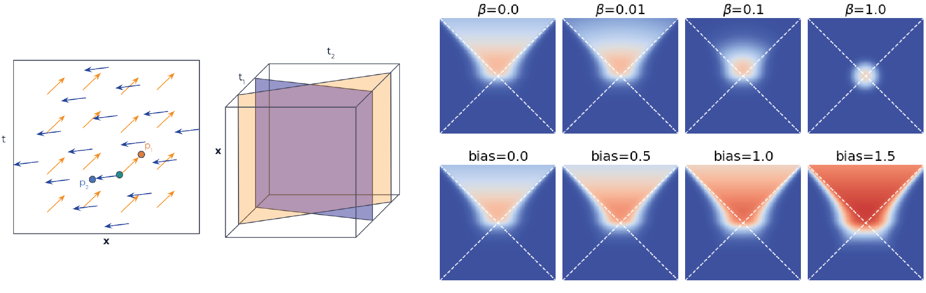
Figure 1: Left/Middle: Relations as diffeomorphisms induced by vector fields, and as spacetime submanifolds of a multi-time manifold. Right top: Interpolated likelihood $\mathcal{F}^{(\beta)}$ (14); Right bottom: Bias effect $\sigma(\operatorname*{\mathrm{logit}}(\mathcal{F})+\mathrm{bias})$ (15). The vertical axis is the timelike dimension for $\mathcal{M}=\mathbb{R}^{1,1}$.

We incorporate multiple relations via a combination of two strategies: 1. Relations as endomorphisms, and 2. relations as spacetime submanifolds of a node embedding manifold with multiple time dimensions. While the latter is specific to pseudo-Riemannian manifolds, the first is widely applied in Riemannian manifold embedding models. Node transformations are just point realizations of endomorphisms and is the method taken by all linear tensor factorization models and embedding models MuRE/MuRP Balažević et al. (2019b). Here we translate the implementation of the latter to pseudo-Riemannian manifolds and empirically validate their applicability when used together with the TFD function (4) to determine the probabilities in (5). Details of these two strategies are given below with an illustration in Figure 1 (left/middle). We also introduce a Wick-rotated regularising Riemannian term and node and relation-specific bias terms, which we describe in more detail in Section 5.4. We will refer to this combined model as PseudoE.

4.1 Relation Embeddings 1: Endomorphisms

The first strategy is to encode relations as node transformations, resulting in relation-specific node embeddings. The framework developed in Balažević et al. (2019b) for Riemannian manifolds is to map each relation to a pair of endomorphisms of $\mathcal{M}$, i.e.

$$r_{k}\,\mapsto\,(f_{k},g_{k}),$$ (8)

where $f_{k},g_{k}:\mathcal{M}\rightarrow\mathcal{M}$ are the node transformations of the respective head and tail nodes in each triple candidate. Adapting the setup for our pseudo-Riemannian case, we replace the squared distance functions with our TFD function (4).

4.1.1 MuRE/P for pseudo-Riemannian manifolds

One candidate for the score function $\phi$ in (5) for a multi-relational knowledge graph given in terms of the single-relation TFD function (4) is

$$\phi_{E}(v_{i},r_{k},v_{j}):=\operatorname*{\mathrm{logit}}\bigl{(}\mathcal{F}(f_{k}(p_{i}),g_{k}(p_{j}))\bigr{)}.$$ (9)

where the subscript E refers to endomorphism. This general definition allows a broad array of design options for $f_{k}$ and $g_{k}$, e.g. non-invertible, non-linear neural networks. In this paper we adapt the two transformation choices from Balažević et al. (2019b) for Riemannian manifold embeddings as follows.

The first transformation is a TransE-like offset where each relation $r_{k}$ is mapped to a vector field $u_{k}$, which when restricted to any node embedding point $p\in\mathcal{M}$ gives the vector that defines the transformation. We have, for all $p\in\mathcal{M}$,

$$f_{k}(p):=\exp_{p}(u_{k}\rvert_{p}),$$ (10)

where $\exp_{p}(*)$ is the exponential map on $\mathcal{M}$ at $p$. There are many ways to parameterize $u_{k}$ depending on the choice of $\mathcal{M}$. In this paper, we keep to the simplest example $\mathcal{M}=\mathbb{R}^{1,n-1}$ where eq. (10) is simply $f_{k}(p)=p+u_{k}\rvert_{p}$, for constant $u_{k}$.

The second transformation is DistMult-like component-wise scaling, where each relation $r_{k}$ is mapped to a diagonal $(1,1)$-tensor $R_{k}\in T_{\mathbf{0}}\mathcal{M}\otimes T_{\mathbf{0}}^{*}\mathcal{M}$ and

$$g_{k}(p):=\exp_{\mathbf{0}}(R_{k}\log_{\mathbf{0}}(p)),$$ (11)

where $\log_{\mathbf{0}}:\mathcal{M}\rightarrow T_{\mathbf{0}}\mathcal{M}$ is the logarithm map. In the example $\mathcal{M}=\mathbb{R}^{1,n-1}$ we have $g_{k}(p)=R_{k}p$.

4.2 Relation Embeddings 2: Spacetime submanifolds

In the previous section, the background geometry was fixed while the node embeddings were mapped to different points under relation-specific endomorphisms. In this section we take the dual view where node embeddings themselves remain fixed while the manifold itself adapts to different relations.

The time displacement is explicitly used by the TFD function to provide a direction to the edges, so for multiple relations we can simply define a manifold with multiple time dimensions and introduce the procedure of a relation-specific time projection. We note that this projection is a specific instance of an endomorphism, one, however, that is necessary for multi-time manifolds. Which is to say, any relation-specific endomorphism on a manifold with multiple time dimensions must define a submanifold with only a single time dimension.

For a knowledge graph with $n_{r}$ relations, let $\mathcal{M}$ be a pseudo-Riemannian manifold with signature $(n_{t},n_{x})$, where $n_{t}>1$. Next, for each relation $r_{k}$ we define a mapping $\tau_{k}:\mathcal{M}\rightarrow\mathcal{M}_{k}$ where $\mathcal{M}_{k}$ is a submanifold of $\mathcal{M}$ with signature $(1,n_{x})$. Then the second candidate for the score function $\phi$ is

$$\phi_{SS}(v_{i},r_{k},v_{j}):=\operatorname*{\mathrm{logit}}\bigl{(}\mathcal{F}(\tau_{k}(p_{i}),\tau_{k}(p_{j})\bigr{)}.$$ (12)

where the subscript SS refers to spacetime submanifold. Just as for the endomorphisms (8), one has great freedom in designing $\tau_{k}$. In this work, we restrict ourselves to the simplest flat case of $\mathcal{M}=\mathbb{R}^{n_{t},n_{x}}$ and for each relation $r_{k}$ we specify a vector $h_{k}\in\mathbb{R}^{n_{t}}$ such that the submanifold map is

$$\tau_{k}:\bigl{(}\mathbf{t},\mathbf{x}\bigr{)}\mapsto\bigl{(}t_{k},\mathbf{x}\bigr{)}\equiv\bigl{(}(h_{k}\cdot\mathbf{t}),\mathbf{x}\bigr{)},$$ (13)

where $\mathbf{t}\in\mathbb{R}^{n_{t}}$ and $\mathbf{x}\in\mathbb{R}^{n_{x}}$ are, respectively, the time and space coordinates of a given node embedding. Following Sim et al. (2021) (eq. 20) we also consider cylindrical Minkowski submanifolds by identifying $t_{k}\sim t_{k}+aC$, for some multiple of the circumference $C\in\mathbb{R}^{+}$.

In this paper we set $n_{t}<n_{r}$, imposing that the time coordinate parameters be shared between relations. In eq. (13), the submanifold time coordinate $t_{k}$ is a linear combination of the multiple time coordinates of the original manifold.

4.3 Wick-rotation regularisation and biases

The lightcone structure of the TFD function (4) may turn out to be too strong of a constraint for certain graph structures (e.g. random geometric graphs) with relations that suit standard Riemannian backgrounds. To accommodate this we consider an interpolation between Riemannian and pseudo-Riemannian structures as follows. For a fixed mixing coefficient $0\leq\beta\leq 1$, we replace the TFD function $\mathcal{F}$ with the weighted geometric mean

$$\mathcal{F}^{(\beta)}:=\mathcal{F}^{1-\beta}\widetilde{F}^{\beta},$$ (14)

where $\widetilde{F}\equiv F_{1}(\tilde{s}^{2})$ is the Fermi-Dirac term from (4) with the squared geodesic distance $\tilde{s}^{2}$ calculated in the Wick-rotated space with metric $\tilde{g}$ (2). In Figure 1 (top right), we plot an illustrative examples of the effect of the mixing; we observe a smooth interpolation between a lightcone structure with sharp boundaries and a Gaussian-like isotropic profile.

The final addition to our model is a set of specific bias terms for the nodes – $b_{i},b_{j}$, and relations – $c_{k}$. The node biases introduced in Balažević et al. (2019b) for Riemannian manifold embeddings were interpreted as defining the size of spheres of influences; in the pseudo-Riemannian case, as shown in Figure 1 (bottom right), the geometrical picture is more akin to cones of influence, where the time/spacelike partition of the manifold, and hence the pseudo-Riemannian embedding model as a whole, is preserved.

Combining the elements of our model – merging $\phi_{E}$ (eq. (9)) and $\phi_{SS}$ (eq. (12)) and including the features in eqs.(13), and (14) – we define our PseudoE score function as

$$\phi(v_{i},r_{k},v_{j})=\operatorname*{\mathrm{logit}}\Bigl{(}\mathcal{F^{(\beta)}}\bigl{[}(f_{k}\circ\tau_{k})(p_{i}),(g_{k}\circ\tau_{k})(p_{j})\bigr{]}\Bigr{)}+b_{i}+b_{j}+c_{k},$$ (15)

where the manifold map is performed after the spacetime projection.

5 Results

In this section we evaluate PseudoE (15) on a standard set of link prediction tasks and demonstrate how its separate components capture different aspects of graph data. For simplicity, we restrict ourselves to the trivial flat pseudo-Riemannian manifolds with metric $g=\operatorname*{\mathrm{diag}}(-1,\dotsc,-1,1,\dotsc,1)$, leaving the study of curved spaces to a later work.

5.1 Experimental Setup

5.1.1 Datasets

We run our experiments on the two standard link prediction datasets: FB15K-237 and WN18RR, as well as the Hetionet scientific knowledge graph Himmelstein and Baranzini (2015). A full description is provided in Appendix A1.

5.1.2 Training

For FB15K-237 and WN18RR, we use the common data augmentation technique Dettmers et al. (2018) of adding reversed triples, i.e. for every $(v_{i},r_{k},v_{j})$ triple that exists, we append $(v_{j},\tilde{r}_{k},v_{i})$. For Hetionet, we follow Nadkarni et al. (2021) and omit this step.

The model is trained by minimizing the negative log-likelihood loss

$$\small\begin{split}\mathcal{L}=-\sum_{\begin{subarray}{c}i,j\in V,k\in R\\ (v_{i},r_{k},v_{j})\in\hat{\mathcal{G}}\end{subarray}}\biggl{[}\log\sigma(\phi(v_{i},r_{k},v_{j}))+\sum_{\begin{subarray}{c}a=1\\ l_{a}\in V\end{subarray}}^{m/2}\log(1-\sigma(\phi(v_{i},r_{k},v_{l_{a}})))+\sum_{\begin{subarray}{c}b=1\\ l_{b}\in V\end{subarray}}^{m/2}\log(1-\sigma(\phi(v_{l_{b}},r_{k},v_{j})))\biggr{]},\end{split}$$ (16)

where $m$ is the even number of random negative node samples ($v_{l_{a}},v_{l_{b}}$) per triple. In the case where data augmentation is performed, we drop the last summation term in (16) and perform all $m$ negative replacements solely on the tail node. We train with minibatch stochastic gradient descent and experiment with both Adam Kingma and Ba (2014) and SM3 Anil et al. (2019) optimizers. All node and relation embeddings are randomly initialised with the normal distribution $N(0,\sigma_{i}^{2})$. We perform early stopping on the evaluation metric (see next section).

We perform a round of hyperparameter tuning via random search over the validation set evaluation metric. The optimal hyperparameters selected from each dataset and model combination are given in Table A2.

5.1.3 Evaluation

We evaluate our models using the mean reciprocal rank (MRR) and the hits@k information retrieval metrics Schütze et al. (2008). Following convention, we use the filtered version of the metric Bordes et al. (2013) where each test set triple is ranked against all others obtained by swapping out the tail node, but excluding those triples that can be found in the full dataset $\hat{\mathcal{G}}$. In the case of Hetionet, in order to compare with the results presented in Nadkarni et al. (2021), we use their predefined fixed-sized ($N=80$) set of negative samples of matching node type for each head-relation pair for both validation and testing.

5.2 Link prediction performance

WN18RR FB15K-237 Hetionet (small) MRR Hits@10 MRR Hits@10 MRR Hits@10 TransE (Bordes et al., 2013) 0.226 0.501 0.294 0.465 0.502 0.798 DistMult (Yang et al., 2015) 0.430 0.490 0.241 0.419 0.460 0.778 ComplEx (Trouillon et al., 2016) 0.440 0.510 0.247 0.428 0.459 0.778 Rescal (Wang et al., 2019) 0.420 0.447 0.270 0.427 – – TuckER (Balažević et al., 2019a) 0.470 0.526 0.358 0.544 – – MuRE Balažević et al. (2019b) 0.475 0.554 0.336 0.521 0.527* 0.809* RotE* Chami et al. (2020) 0.494 0.585 0.346 0.538 – – AttE* Chami et al. (2020) 0.490 0.581 0.351 0.543 – – MuRP Balažević et al. (2019b) 0.481 0.566 0.335 0.518 – – RotH* Chami et al. (2020) 0.496 0.586 0.344 0.535 – – AttH* Chami et al. (2020) 0.486 0.573 0.348 0.568 – – PseudoE (MT only) 0.314 0.433 0.273 0.451 0.543 0.812 PseudoE (DT only) 0.474 0.567 0.351 0.539 0.538 0.813 PseudoE (both) 0.473 0.565 0.351 0.536 0.544 0.813

Table 1: Link prediction results. Best performance by metric is in bold, and the highest performing PseudoE variant is shaded in gray. Hetionet baselines are taken from Nadkarni et al. (2021) with the exception of MuRE which is PseudoE run with $\beta=1$. DT: DistMult-TransE scoring function, MT: multi-time relations. *Shown here are the best results by dataset of the RotE/H, RefE/H and AttE/H variants Chami et al. (2020).

We run our series of link prediction experiments testing three separate PseudoE variants – one with the DistMult-TransE endomorphism only (DT), one with submanifolds of multi-time manifolds only (MT), and one with both implementations. We compare these to several common tensor factorization baselines, as well as the MuRE/P and AttE/H embedding models. The results are shown in Table 1.

PseudoE is highly competitive on all three datasets, coming in either top by a good margin (Hetionet) or 2nd/3rd (FB15K-237 and WN18RR) among the comparable flat-space and linear models. For FB15K-237 specifically, it was first speculated in Balažević et al. (2019b) that the relatively large number of relations benefit from the parameter sharing feature of the relational embeddings in TuckER, the most performant model. Therefore, the close performance of PseudoE demonstrates its ability to model a large number of relations without either explicit parameter sharing or, in our implementation, curved geometries.

Next, it is clear from the model ablation results comparing MT, DT, and both model components together that the best combination of methods for encoding relations is highly dependent on the dataset used. For instance, the spacetime submanifold model performs poorly on both WN18RR and FB15K-237, but for Hetionet, it outperforms the endomorphism approach, with the combination of the two being the optimal setup. An obvious extension of this work would be to explore more expressive multi-time projections to explore the broader impact of this model feature on datasets beyond Hetionet.

Finally, we note that the single-relation pseudo-Riemannian baseline in Sim et al. (2021) cannot do better than an assignment of relation types according to the frequencies observed in the training data. Even assuming perfect classification of edges vs. non-edges, the performances on both WN18RR and FB15K-237 datasets would be close to random.

5.3 Interpolating between geometries with $\beta$

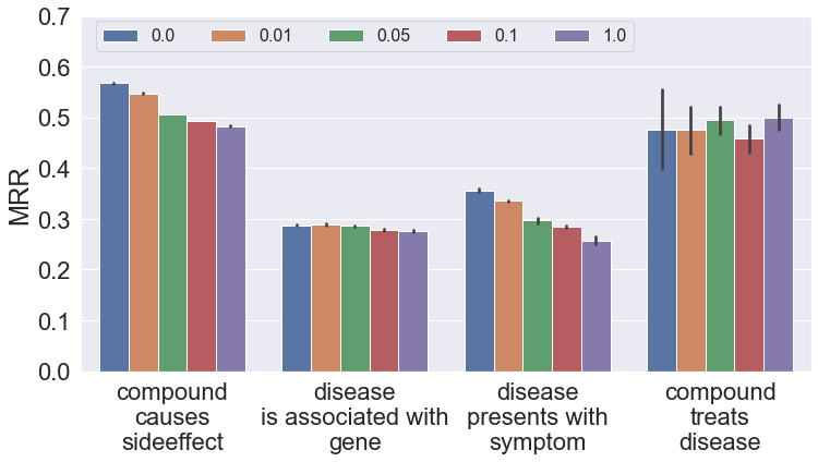
Figure 2: MRR by relation, varying the mixing coefficient from $\beta=0$ (Minkowski) to $\beta=1$ (Euclidean), on Hetionet. Error bars represent $\pm 1$ s.d. across four runs.

In this section, we explore the effect of varying the weight coefficient $\beta$ (14) on link prediction performance. We found that the effect of the mixing parameter, assessed on an initial run of the DT model using smaller embedding size (d=200), was positive. For WN18RR, we achieve an MRR=0.472 ($\beta>$0) vs. 0.445 ($\beta$=0, i.e. no mixing). FB15-237 we achieve MRR=0.347 ($\beta>$0) vs. 0.318 ($\beta$=0). The highest performing PseudoE models on WN18RR, FB15K-237, and Hetionet in Table 1 had $\beta=0.18,\,0.30,\,\text{and}\,0.03$ respectively. The relatively high value for FB15K-237 is not unsurprising given that it is a large heterogeneous knowledge graph with a large number of similarity-type relations for which a sharp lightcone likelihood profile may not be appropriate.

We now observe how the relative contributions of a Minkowski geometry ($\beta=0$) vs. its Wick-rotated Euclidean ($\beta=1$) geometry affect the prediction of individual triples with the various directed or symmetric relations in Hetionet (Figure 2). Notably, for the directed relations causes and presents with, we observe a clear drop in performance as the pseudo-Riemannian TFD likelihood function (4) gives way to an increasingly isotropic form (see Figure 1 right). As the TFD function is designed specifically for such relations with non-metric properties Sim et al. (2021), it is a validation that the pseudo-Riemannian model outperforms on these specific relations. On the contrary, varying $\beta$ has a negligible impact on the performance of the undirected is associated with relationship predictions. Finally, we note that the performance on the treats relation is inconclusive, due to the small number of edges for this relation in the dataset ($N_{\text{treats}}=597$ vs. $N_{\text{causes}}=110569$).

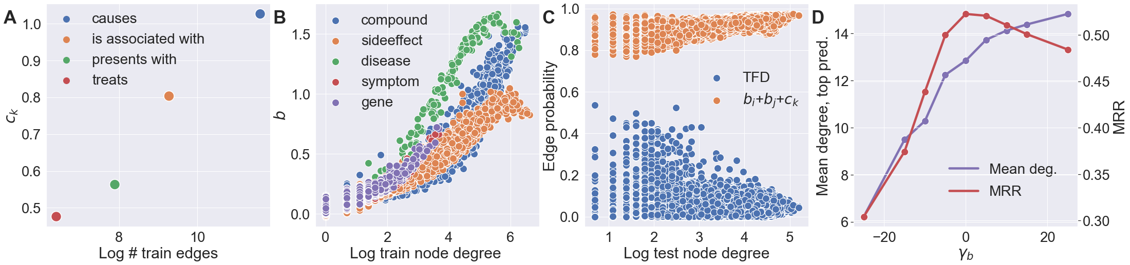
Figure 3: A: Relation bias terms $c_{k}$ vs. edge count. B: Node bias term $b$ vs. node degree. C: Components of the composite score – the TFD component and the combined bias terms $b_{i}+b_{j}+c_{k}$ – vs. edge probability. D: Average degree of top-ranking prediction, scaling the target bias via $\gamma_{b}$.

5.4 Removing bias from KG link predictions

We explore the role that $c_{k}$, $b_{i}$, and $b_{j}$ (15) play in disentangling the dataset biases related to relation prevalence and node degrees from our predictions. On the model trained on Hetionet, we observe a positive log-linear relationship between $c_{k}$ and the relation prevalence (Figure 3A), and a similarly positive relationship between the combined node biases $b=b_{i}+b_{j}$ and node degree across all five node types (Figure 3B). Importantly, Figure 3C shows a strong positive correlation (Pearson’s r) between node degree and the node bias component of edge probability ($r(15566)=0.69$, $p<.001$), versus a negligible negative relationship ($r(15566)=-0.05$, $p<.001$) between the TFD component. This ability offers an opportunity to factor out the node degree-bias of link predictions in a principled way at test time. We explore the application of this scaling to gene prioritization in drug target identification in Appendix Section C.

6 Summary

In this paper we introduced PseudoE, an extension of pseudo-Riemannian embeddings to multiple relations. For link prediction, PseudoE is competitive on FB15K-237 and WN18RR, and is state of the art amongst linear models on a subset of the Hetionet dataset. This work can be extended to curved pseudo-Riemannian manifolds and applied to a broader set of applications such as node classification.

A Datasets

A.1 FB15K-237

FB15K Bordes et al. [2013] is a subset of the Freebase dataset Bollacker et al. [2008], a collection of triples representing general history facts. FB15K-237 Toutanova et al. [2015] is the subset of FB15K where, to minimize data leakage, all triples with trivial inverse relations of training relations are removed from the validation and test sets.

A.2 WN18RR

WordNet Miller [1995] is an acyclic, hierarchical, tree-like network of nouns, each with relatively few ancestors and many descendants. WN18RR Dettmers et al. [2018], a subset of WordNet, is comprised of eleven relations, and, similar to FB15K-237, is cleaned for inverse relation test set leakage.

A.3 Hetionet (small)

Hetionet is a biomedical dataset that integrates several publicly-available scientific databases, including the Unified Medical Language System (UMLS) Bodenreider [2004], GeneOntology Ashburner et al. [2000], and DisGenNET Piñero et al. [2016]. In order to facilitate comparison of performance metrics, we restrict Hetionet to the subset used in Nadkarni et al. [2021] and Alshahrani et al. [2021] – referred to here as “Hetionet (small)” – that includes four relations, (treats, presents, associates, and causes), linking five entity classes (compounds, diseases, genes, side effects, and symptoms) in a directed acyclic graph.

			# Edges
	# Ent.	# Rel.	Train	Valid	Test
FB15K-237	14,541	237	272,114	17,534	20,465
WN18RR	40,943	11	86,836	3,033	3,133
Hetionet (small)	12,733	4	124,543	15,566	15,567

Table A1: Dataset specificiation for link prediction task.

B Training hyperparameters

Hyperparameters below relate to the models in Table 1. These hyperparameters were selected based on random search maximising the validation MRR.

Model PseudoE (MT only) PseudoE (DT only) PseudoE (both) Dataset Wordnet FB15K Hetionet Wordnet FB15K Hetionet Wordnet FB15K Hetionet $\alpha$ 0.3673 0.136206 0.10124 0.3673 0.136206 0.10124 0.3673 0.136206 0.10124 $\alpha^{\prime}$ 0.75182 0.971685 1.0 0.75182 0.971685 1.0 0.75182 0.971685 1.0 $u$ 0.040226 0.09592 0.03 0.040226 0.09592 0.03 0.040226 0.09592 0.03 $\tau_{1}$ 0.29015 0.129815 0.11071 0.29015 0.129815 0.11071 0.29015 0.129815 0.11071 $\tau_{2}$ 0.21697 0.086457 0.06277 0.21697 0.086457 0.06277 0.21697 0.086457 0.06277 $n_{x}$ 500 200 200 500 500 200 500 500 200 $n_{t}-1$ 40 40 1 0 0 0 1 2 1 $\beta$ 0.18 0.0 0.0 0.18 0.15 0.0 0.18 0.15 0.0 circumference - - - - 8.0 8.0 - - 6.0 $\sigma_{i}$ init scale 0.001 0.001 0.02255 0.001 0.001 0.02255 0.001 0.001 0.02255 Learning rate 0.08 0.1 0.0002 0.08 0.0001 0.0002 0.08 0.0001 0.0002 Batch size 128 128 100 128 128 100 128 128 100 Negative samples $m$ 50 50 20 50 50 20 50 50 20 optimizer SM3 SM3 Adam SM3 Adam Adam Adam Adam Adam 1

Table A2: Optimal model and training hyperparameters.

We observe that sensitivity to specific hyperparameters is highly dataset-specific, with WN18RR being the dataset that required the most careful tuning. However, we note that this sensitivity is not unique to PseudoE and we observe very similar optimization challenges when reproducing the results of MuRE/P. Also, we note that many of the parameters are common to many models – for instance $\tau_{1}$ and $\tau_{2}$ are analogous to the softmax temperature and $u$ to a loss-margin radius – or involved in parameterizing the geometry. There are, in effect, just two additional hyperparameters specific to PseudoE: the mixing parameter $\beta$, and $n_{t}$, the number of time dimensions.

C Qualitative assessment of gene precedence with varying bias

The negligible correlation of the TFD term with node degree, discussed in Section 5.4 offers an opportunity to factor out the node degree-bias of link predictions in a principled way – at test time, one simply scales the appropriate bias terms to up- or down-weight those predictions that are poorly- or well-connected respectively, i.e.

$$b_{i}\rightarrow\gamma_{b}b_{i},$$ (17)

for some scaling factor $\gamma_{b}\in\mathbb{R}.$

In Figure 3D we see that tuning the target bias varies the mean node degree of the top gene prediction across all test-set diseases in Hetionet. This allows us to variably prioritize either those genes that are novel and poorly connected (low $\gamma_{b}$) or are well studied and widely connected (high $\gamma_{b}$), trading off model performance for prediction novelty. A real-world application for this capability is in the area of gene prioritization in commercial drug discovery, as biologists seek out genes that are plausibly implicated in a particular disease (high model performance) while being both safe to target and novel, i.e. not being involved in many biological processes, or already targeted for treatment (low node degree in the knowledge graph).

Taking breast cancer as an example, Table A3 shows the 10 top-ranking associated genes for three levels of $\gamma_{b}$. Through target triage, similar to the process described in Paliwal et al. [2020], we annotated those targets that were non-specific cancer genes, those targets specific to breast cancer, those targets that are interesting and understudied to date, and those targets that were irrelevant. What is immediately noteworthy about the $\gamma_{b}=25$ list is the prevalence of generic cancer genes, like TNF and TP53. While the $\gamma_{b}=1$ case – the original trained model – unearths disease-specific genes, such as RAD51, the $\gamma_{b}=-25$ case reveals a handful of genes that are understudied (i.e. low degree) yet interesting, like DTX3 or RPS6KB2, with plausible or preliminary existing links to breast cancer, making them of particular interest in the context of drug discovery.

Rank	$\gamma_{b}=25$	$\gamma_{b}=1$	$\gamma_{b}=-25$
1	TNF	COL7A1	DTX3 $\bigstar$
2	TP53	RAD51 $\blacksquare$	MRPS23 $\bigstar$
3	PTGS2	SYNJ2 $\blacksquare$	RPS6KB2 $\bigstar$
4	IL6	SLC39A7	ABRAXAS1 $\bigstar$
5	MMP9	MRE11 $\blacksquare$	CDA
6	ALB $\times$	FGF3	MAP2K7
7	CXCL8	SFRP1 $\blacksquare$	PCDHGB6 $\times$
8	IL2	UBE2C $\blacksquare$	ESRRA $\times$
9	AKT1	TENT5A $\times$	RBM3 $\bigstar$
10	TGFB1	BABAM1 $\blacksquare$	S100A4

Table A3: Gene prioritization for breast cancer (BC). $\gamma_{b}=1$ is the original model. Shaded cells: generic cancer genes. $\blacksquare$: genes well-studied and established as linked to BC, $\times$: genes irrelevant/uninteresting for BC, $\bigstar$: genes relevant, interesting, and surprising for BC therapy research.

References

- Alshahrani et al. (2021) Mona Alshahrani, Maha A Thafar, and Magbubah Essack. Application and evaluation of knowledge graph embeddings in biomedical data. PeerJ Computer Science, 7:e341, 2021.
- Anil et al. (2019) Rohan Anil, Vineet Gupta, Tomer Koren, and Yoram Singer. Memory-efficient adaptive optimization. arXiv preprint arXiv:1901.11150, 2019.
- Ashburner et al. (2000) Michael Ashburner, Catherine A Ball, Judith A Blake, David Botstein, Heather Butler, J Michael Cherry, Allan P Davis, Kara Dolinski, Selina S Dwight, Janan T Eppig, et al. Gene ontology: tool for the unification of biology. Nature genetics, 25(1):25–29, 2000.
- Balažević et al. (2019a) Ivana Balažević, Carl Allen, and Timothy Hospedales. TuckER: Tensor factorization for knowledge graph completion. In Proceedings of the 2019 Conference on Empirical Methods in Natural Language Processing and the 9th International Joint Conference on Natural Language Processing (EMNLP-IJCNLP), pages 5185–5194, Hong Kong, China, November 2019a. Association for Computational Linguistics. doi: 10.18653/v1/D19-1522.
- Balažević et al. (2019b) Ivana Balažević, Carl Allen, and Timothy M. Hospedales. Multi-relational poincaré graph embeddings. CoRR, abs/1905.09791, 2019b.
- Bodenreider (2004) Olivier Bodenreider. The unified medical language system (umls): integrating biomedical terminology. Nucleic acids research, 32(suppl_1):D267–D270, 2004.
- Bollacker et al. (2008) Kurt Bollacker, Colin Evans, Praveen Paritosh, Tim Sturge, and Jamie Taylor. Freebase: A collaboratively created graph database for structuring human knowledge. In Proceedings of the 2008 ACM SIGMOD International Conference on Management of Data, SIGMOD ’08, page 1247–1250, New York, NY, USA, 2008. Association for Computing Machinery. ISBN 9781605581026. doi: 10.1145/1376616.1376746.
- Bordes et al. (2013) Antoine Bordes, Nicolas Usunier, Alberto Garcia-Duran, Jason Weston, and Oksana Yakhnenko. Translating embeddings for modeling multi-relational data. In C. J. C. Burges, L. Bottou, M. Welling, Z. Ghahramani, and K. Q. Weinberger, editors, Advances in Neural Information Processing Systems, volume 26. Curran Associates, Inc., 2013.
- Chami et al. (2020) Ines Chami, Adva Wolf, Da-Cheng Juan, Frederic Sala, Sujith Ravi, and Christopher Ré. Low-dimensional hyperbolic knowledge graph embeddings. In Proceedings of the 58th Annual Meeting of the Association for Computational Linguistics, pages 6901–6914, Online, July 2020. Association for Computational Linguistics. doi: 10.18653/v1/2020.acl-main.617. URL https://aclanthology.org/2020.acl-main.617.
- Clough and Evans (2017) James R. Clough and Tim S. Evans. Embedding graphs in Lorentzian spacetime. PLOS ONE, 12(11):e0187301, 2017.
- Dettmers et al. (2018) Tim Dettmers, Pasquale Minervini, Pontus Stenetorp, and Sebastian Riedel. Convolutional 2d knowledge graph embeddings. In Thirty-second AAAI conference on artificial intelligence, 2018.
- Gao et al. (2018) Tingran Gao, Lek-Heng Lim, and Ke Ye. Semi-Riemannian Manifold Optimization. arXiv, 2018.
- Gu et al. (2018) Albert Gu, Frederic Sala, Beliz Gunel, and Christopher Ré. Learning mixed-curvature representations in product spaces. In International Conference on Learning Representations, 2018.
- Himmelstein and Baranzini (2015) Daniel S Himmelstein and Sergio E Baranzini. Heterogeneous network edge prediction: a data integration approach to prioritize disease-associated genes. PLoS computational biology, 11(7):e1004259, 2015.
- Kingma and Ba (2014) Diederik P Kingma and Jimmy Ba. Adam: A method for stochastic optimization. arXiv preprint arXiv:1412.6980, 2014.
- Krioukov et al. (2010) Dmitri Krioukov, Fragkiskos Papadopoulos, Maksim Kitsak, Amin Vahdat, and Marián Boguñá. Hyperbolic geometry of complex networks. Phys. Rev. E, 82:036106, Sep 2010.
- Krioukov et al. (2012) Dmitri Krioukov, Maksim Kitsak, Robert S Sinkovits, David Rideout, David Meyer, and Marián Boguñá. Network cosmology. Scientific reports, 2(1):1–6, 2012.
- Law and Stam (2020) Marc T. Law and Jos Stam. Ultrahyperbolic representation learning. In Hugo Larochelle, Marc’Aurelio Ranzato, Raia Hadsell, Maria-Florina Balcan, and Hsuan-Tien Lin, editors, Advances in Neural Information Processing Systems 33, 2020.
- López et al. (2021) Federico López, Beatrice Pozzetti, Steve Trettel, Michael Strube, and Anna Wienhard. Symmetric spaces for graph embeddings: A finsler-riemannian approach. arXiv preprint arXiv:2106.04941, 2021.
- Miller (1995) George A Miller. Wordnet: a lexical database for english. Communications of the ACM, 38(11):39–41, 1995.
- Nadkarni et al. (2021) Rahul Nadkarni, David Wadden, Iz Beltagy, Noah Smith, Hannaneh Hajishirzi, and Tom Hope. Scientific language models for biomedical knowledge base completion: An empirical study. In 3rd Conference on Automated Knowledge Base Construction, 2021.
- Nickel et al. (2011) Maximilian Nickel, Volker Tresp, and Hans-Peter Kriegel. A three-way model for collective learning on multi-relational data. In Lise Getoor and Tobias Scheffer, editors, Proceedings of the 28th International Conference on Machine Learning, pages 809–816, 2011.
- Nickel et al. (2015) Maximilian Nickel, Kevin Murphy, Volker Tresp, and Evgeniy Gabrilovich. A review of relational machine learning for knowledge graphs. Proceedings of the IEEE, 104(1):11–33, 2015.
- Nickel and Kiela (2017) Maximillian Nickel and Douwe Kiela. Poincaré embeddings for learning hierarchical representations. In I. Guyon, U. V. Luxburg, S. Bengio, H. Wallach, R. Fergus, S. Vishwanathan, and R. Garnett, editors, Advances in Neural Information Processing Systems 30, pages 6338–6347, 2017.
- Nickel and Kiela (2018) Maximillian Nickel and Douwe Kiela. Learning continuous hierarchies in the Lorentz model of hyperbolic geometry. In Jennifer Dy and Andreas Krause, editors, Proceedings of the 35th International Conference on Machine Learning, volume 80, pages 3779–3788, 2018.
- Paliwal et al. (2020) Saee Paliwal, Alex de Giorgio, Daniel Neil, Jean-Baptiste Michel, and Alix MB Lacoste. Preclinical validation of therapeutic targets predicted by tensor factorization on heterogeneous graphs. Scientific reports, 10(1):1–19, 2020.
- Piñero et al. (2016) Janet Piñero, Àlex Bravo, Núria Queralt-Rosinach, Alba Gutiérrez-Sacristán, Jordi Deu-Pons, Emilio Centeno, Javier García-García, Ferran Sanz, and Laura I Furlong. Disgenet: a comprehensive platform integrating information on human disease-associated genes and variants. Nucleic acids research, page gkw943, 2016.
- Schütze et al. (2008) Hinrich Schütze, Christopher D Manning, and Prabhakar Raghavan. Introduction to information retrieval, volume 39. Cambridge University Press Cambridge, 2008.
- Seshadhri et al. (2020) C Seshadhri, Aneesh Sharma, Andrew Stolman, and Ashish Goel. The impossibility of low-rank representations for triangle-rich complex networks. Proceedings of the National Academy of Sciences, 117(11):5631–5637, 2020.
- Sim et al. (2021) Aaron Sim, Maciej Wiatrak, Angus Brayne, Páidí Creed, and Saee Paliwal. Directed graph embeddings in pseudo-riemannian manifolds, 2021.
- Sun et al. (2015) Ke Sun, Jun Wang, Alexandros Kalousis, and Stephane Marchand-Maillet. Space-time local embeddings. In C. Cortes, N. Lawrence, D. Lee, M. Sugiyama, and R. Garnett, editors, Advances in Neural Information Processing Systems 28, pages 100–108, 2015.
- Suzuki et al. (2019) Ryota Suzuki, Ryusuke Takahama, and Shun Onoda. Hyperbolic disk embeddings for directed acyclic graphs. In Kamalika Chaudhuri and Ruslan Salakhutdinov, editors, Proceedings of the 36th International Conference on Machine Learning, pages 6066–6075, 2019.
- Toutanova et al. (2015) Kristina Toutanova, Danqi Chen, Patrick Pantel, Hoifung Poon, Pallavi Choudhury, and Michael Gamon. Representing text for joint embedding of text and knowledge bases. In Proceedings of the 2015 Conference on Empirical Methods in Natural Language Processing, pages 1499–1509, Lisbon, Portugal, September 2015. Association for Computational Linguistics. doi: 10.18653/v1/D15-1174.
- Trouillon et al. (2016) Théo Trouillon, Johannes Welbl, Sebastian Riedel, Eric Gaussier, and Guillaume Bouchard. Complex embeddings for simple link prediction. In Maria Florina Balcan and Kilian Q. Weinberger, editors, Proceedings of the 33rd International Conference on Machine Learning, pages 2071–2080, 2016.
- Visser (2017) Matt Visser. How to Wick rotate generic curved spacetime. arXiv, 2017.
- Wang et al. (2019) Yanjie Wang, Daniel Ruffinelli, Rainer Gemulla, Samuel Broscheit, and Christian Meilicke. On evaluating embedding models for knowledge base completion. In Proceedings of the 4th Workshop on Representation Learning for NLP (RepL4NLP-2019), pages 104–112, Florence, Italy, August 2019. Association for Computational Linguistics. doi: 10.18653/v1/W19-4313.
- Yang et al. (2015) Bishan Yang, Wen-tau Yih, Xiaodong He, Jianfeng Gao, and Li Deng. Embedding entities and relations for learning and inference in knowledge bases. In Interrnational Conference on Learning Representations, 2015.