Runtime and Memory Efficient Multi-Objective A*
Abstract
The Multi-Objective Shortest Path Problem (MO-SPP), typically posed on a graph, determines a set of paths from a start vertex to a destination vertex while optimizing multiple objectives. In general, there does not exist a single solution path that can simultaneously optimize all the objectives and the problem thus seeks to find a set of so-called Pareto-optimal solutions. To address this problem, several Multi-Objective A* (MOA*) algorithms were recently developed to quickly compute solutions with quality guarantees. However, these MOA* algorithms often suffer from high memory usage, especially when the branching factor (i.e. the number of neighbors of any vertex) of the graph is large. This work thus aims at reducing the high memory consumption of MOA* with little increase in the runtime. By generalizing and unifying several single- and multi-objective search algorithms, we develop the Runtime and Memory Efficient MOA* (RME-MOA*) approach, which can balance between runtime and memory efficiency by tuning two user-defined hyper-parameters.
I Introduction
Given a graph, the Shortest Path Problem (SPP) involves finding a solution path from a start vertex to a destination vertex with the least cumulative path cost. As a natural extension of the SPP, the Multi-Objective Shortest Path Problem (MO-SPP) associates edges with cost vectors instead of scalar costs, where each element of the vector represents an objective to be optimized. This problem arises in applications such as hazardous material transportation [1] where multiple objectives are optimized simultaneously. Instead, the MO-SPP attempts to find a set of Pareto-optimal (also called non-dominated) solution paths, and the corresponding set of cost vectors is often referred to as the Pareto-optimal front. MO-SPP is computationally challenging as the number of Pareto-optimal paths can grow exponentially with respect to the size of the graph even with two objectives [2].
To compute the Pareto-optimal front, on the one hand, a family of MOA* algorithms were developed to quickly find the exact [3, 4, 5, 6] or approximated [7, 8, 9] Pareto-optimal front, and this work limits its focus to the exact algorithms. However, these algorithms primarily focus on the runtime efficiency and can consume a lot of memory during the search, especially in graphs with large branching factors (average number of successors per vertex), such as the state lattice graphs used in robotics [10], which limits their potential usage on platforms with limited computational resources (e.g. mobile robots, quadrotors). On the other hand, while being able to provide theoretic guarantees on memory consumption, existing memory-efficient MOA* algorithms [11, 12] either make assumptions on the form of the input graph (e.g. acyclic graph), or sacrifice the runtime efficiency significantly, which hinders their practical usage in large graphs or dense state lattices in robotics [10]. This work thus develops a new algorithm, called Runtime- and Memory-Efficient MOA* (RME-MOA*) that balances runtime and memory efficiency by leveraging several techniques from previous works.
RME-MOA* has three distinct features: Firstly, its search framework is based on our prior EMOA* [6], a runtime-efficient MOA* algorithm Secondly, it extends the partial expansion technique [13] from the single- to multi-objective case and fuses it with EMOA* in order to trade off runtime for memory efficiency. Finally, RME-MOA* leverages PIDMOA* [11], a memory-efficient iterative deepening depth-first MOA* algorithm, by switching between best-first search, as in EMOA*, and iterative depth-first search, as in PIDMOA*, to further improve memory efficiency. We show that the proposed RME-MOA* is a strict generalization of EMOA* and PIDMOA* and can move along a spectrum from runtime efficient (EMOA*) to memory efficient (PIDMOA*) by tuning two user-defined hyper-parameters that control the search process.
Our RME-MOA* is guaranteed to find the Pareto-optimal solution front. We test our RME-MOA* in both grid-like graphs with varying branching factors and robot state lattices against two baselines: its predecessors EMOA* and PIDMOA*. RME-MOA* is able to significantly reduce memory consumption compared to EMOA*, at the expense runtime performance, on problem instances with large branching factors. RME-MOA* is also able to significantly increase runtime performance compared to PIDMOA* at the expense of memory efficiency.
II Problem Description
Let denote a directed graph, where is a set of vertices, a set of directed edges connecting those vertices, and a cost function that maps edges to non-negative cost vectors, where is the number of objectives to be minimized. Let be the successor vertices in graph of vertex .
Let be a path in from to , which is a sequence of vertices such that for all . Let and denote the start and destination vertex respectively. We call a path from the start vertex to some arbitrary vertex a partial path. Every path is associated with a vector path cost where . To compare two paths, we compare their corresponding cost vectors using the notion of dominance [14]. Given with denoting the -th component of , dominates ()111In the literature, dominates and weakly dominates are sometimes also denoted as and , respectively [6]. We choose to use notation and (as in [11]) as it reads more intuitively and alleviates confusion with lexicographic ordering (). iff . Similarly, weakly dominates () iff .
Let and be two distinct paths from to . dominates () iff , and weakly dominates () iff . Note in the case where and , the paths are solution paths from the start vertex to the destination vertex. In the MO-SPP, a Pareto-optimal solution is a path that is not dominated by any other path in (i.e. for all in ). The set of all such paths is the exact Pareto-optimal (or non-dominated) solution set. Any maximal subset of the Pareto-optimal solution set where any two paths in do not have the same cost is known as a maximal cost-unique Pareto-optimal solution set. The goal of this work is to find a maximal cost-unique Pareto-optimal solution set for the MO-SPP.
III Preliminaries
III-A Notation and Terminology
Let be a heuristic function mapping vertices to heuristic vectors, where is an under-estimate of the true optimal path cost from to . Our algorithm, as well as its predecessors [6, 4, 3] rely on the heuristic being consistent: is consistent iff . This guarantees that does not overestimate the cost between any two adjacent vertices. Let denote the lower bound on the vector cost of any solution path that proceeds from partial path .
Let a label represent a partial path .222To identify a partial path, different names such as nodes [4], states [15] and labels [16, 17] have been used in the multi-objective path-planning literature. This work uses “labels” to identify partial solution paths. A label is expanded when the corresponding partial path is extended to all successors of . A label is dominated (or weakly dominated) iff the corresponding partial path is dominated (or weakly dominated). Let , , , and be the parent label that was expanded to create . Let be the children labels of parent label that are created on expansion of . Let OPEN be an ordered list of labels, implemented as a priority queue, where labels are ordered lexicographically by . Let CLOSED denote a set of labels that have been expanded. Let be the Pareto frontier at vertex , i.e. the set of all non-dominated partial path costs (and their associated labels) found so far during the MOA* search from to . We say dominates (or weakly dominates) , iff s.t. (or ), which is denoted as (or )). Let be the Pareto-optimal solution frontier, which, when the search terminates, is a maximal cost-unique Pareto-optimal solution set.
III-B EMOA*
Because we base RME-MOA* on EMOA*’s search framework, we elaborate EMOA* here, referring to Algorithms 1,2, and 3 in [6] to save space. At first, a label for the start vertex is created and added to OPEN. The main loop then iteratively extracts from OPEN a label with the lexicographically smallest . The extracted label is then checked for dominance: if or , which are called FrontierCheck and SolutionCheck, respectively (Alg. 2 in [6]). If is not weakly dominated by either or , then, a procedure called UpdateFrontier is invoked (Alg. 3 in [6]), where is added to , and all labels in whose are dominated by are filtered. Then, is expanded, and for each newly generated label dominance checks are performed to determine if either or . If not, then is added to OPEN. The search terminates when OPEN is empty, which guarantees that is a maximal cost-unique Pareto optimal solution set.
The frequent dominance checks during MOA* search pose a computational challenge, which EMOA* addresses in three ways. Firstly, it uses “dimensionality reduction” [3] to reduce the number and dimension of cost vector comparisons in each Check and Filter operation [6]. These operations are additionally sped up by using a balanced binary search tree (BBST) to represent at each , which further reduces the number of vector comparisons per operation. Finally, EMOA* leverages the notion of “lazy checks” from [4] to defer the dominance checks of a label until just before its expansion, which removes the need to explicitly filter OPEN after each label generation. We refer the reader to [6] for a more detailed explanation of these techniques. While these improvements help in improving runtime performance, EMOA* still suffers from high memory consumption.
III-C PIDMOA*
Unlike EMOA*, which addresses the high runtime expense of the MO-SPP, PIDMOA* [11] attempts to do so for memory consumption. An extension of Iterative Deepening A* (IDA*) [18] to the multi-objective case, PIDMOA* uses the same strategy of performing DFS up to a threshold and iteratively increasing the threshold after each search iteration until the optimal solution is found. Instead of a scalar cost threshold as in IDA*, however, PIDMOA* maintains a Pareto threshold set () of cost vectors. Search is terminated at any partial path where or , where, just as in EMOA*, is the Pareto-frontier maintained at the destination vertex. PIDMOA* is designed to consume memory linear to the depth and number of the solutions, as DFS only explicitly maintains the current path (and all found solutions) during search. Notably, PIDMOA* does not maintain a CLOSED set, as EMOA* does in the form of . As a result, however, its runtime increases dramatically with the depth of the solutions. Refer to [11] for a more detailed explanation of the original algorithm.
III-D PEA*
Our method leverages the partial expansion technique described in [13]. Different from A*, Partial Expansion A* (PEA*) only explores a subset of successors of when expanding and reserves the remaining successors for future expansion by re-inserting their predecessor into OPEN with an “updated value”, which we call its re-expansion value .333In [13], of a vertex is called the stored value of and denoted . We change notation to and the name to re-expansion value to alleviate potential confusion between and and clarify the purpose of the value. To expand a vertex , PEA* explores only the subset of the successors of that satisfy with being a scalar constant hyperparameter that parameterizes the “amount” of partial expansion, which we explain later. All successors that satisfy this condition are explored and are expanded as in regular A*. The other successors that do not satisfy this condition are unexplored and are reserved for future re-expansion by re-inserting into OPEN (now ordered by instead of ) with an updated for all unexplored successors of . is later re-expanded one or more times until all its successors have been explored. PEA* is thus able to trade off runtime (increased number of (re)expansions) for memory efficiency (less explored successors per (re)expansion, resulting in a smaller maximal size of OPEN). This tradeoff is parameterized by , where small values of correspond to less explored successors per (re)expansion and more (re)expansions overall, and sufficiently large values behave identically to A*. PEA* has been shown to be memory efficient for large branching factors problems, claiming to reduce memory consumption by a factor of the branching factor . This is because PEA* reduces the size of OPEN by, at most, a factor of because the ratio of OPEN to CLOSED is, at most, to in traditional A* [13]. Notably, PEA* does not reduce the size of the CLOSED set and so is less effective on small branching factor problems, where the ratio of OPEN to CLOSED is small.
IV Method
| new label: , , , |
| new label: , , , |
| new label: , , |
IV-A New Concepts
Let be the -dimensional re-expansion vector associated with a label . As with in PEA*, is used to efficiently “store” information about the children of to determine when it is necessary to re-expand . Let be lexicographic comparison operators between two vectors. On label generation, , and at the end of each (re)expansion, for all unexplored children , defined as follows: For each (re)expansion of , let be the explored children of . Let be the unexplored children of .444In [13], these explored and unexplored sets of children are called promising and unpromising, respectively. We change semantics here because the relative “ promise” of one label vs another is not obvious for multi-objective costs and lexicographic ordering does not fully capture this notion. Let be a user-defined constant vector that parameterizes the degree of partial expansion, as in PEA*. Let be the previously explored children of , which will always be on first expansion of .
Let be another user-defined constant vector that parameterizes the “distance” from the goal vertex at which to start PIDMOA* search, where distance from to is estimated by (to avoid confusion, we call the start vertex for each PIDMOA* iteration instead of ). Let OPEN_DFS be a stack that stores labels in Last-In First-Out (LIFO) order. Let be the current Pareto threshold frontier maintained during each PIDMOA* search iteration, and let be the Pareto threshold frontier for the next search iteration.
For all , let be the PIDMOA* path of , or the portion of the path found during PIDMOA* search.
IV-B Algorithm Overview
Alg. 1 depicts the pseudocode for RME-MOA*, and it follows a similar framework to that described in Sec. III-B. In each RME-MOA* iteration (lines 5-31), label with the lexicographically smallest is extracted from OPEN (line 6). As in EMOA*, FrontierCheck and SolutionCheck are performed, but now is checked before deciding whether to call the new operation UpdateSolution or UpdateFrontier (lines 7-12). FrontierCheck and UpdateFrontier are additionally modified such that, if has been added to before, FrontierCheck returns false, and UpdateFrontier does not modify These modifications are discussed in Sec. IV-C2. On lines 13-14, if is within a certain distance of for all cost functions (i.e. ), is now expanded using a modified PIDMOA* search, depicted in Alg. 2 (discussion in Sec. IV-C3). This is done in an effort to save memory while avoiding the steep runtime cost of a deep PIDMOA* search. Otherwise, is expanded using partial expansion. For all , only those that satisfy what we call the partial expansion check (lines 18-27) are explored and added to the OPEN (discussed in Sec. IV-C1). If, after expansion, has any remaining unexplored children, is added back to OPEN with for re-expansion (lines 16, 25, 28-30). The search process iterates until OPEN depletes. At termination, is returned (line 31), which is guaranteed to be a maximal cost-unique Pareto-optimal solution set (Sec. V).
IV-C Key Procedures and Discussion
IV-C1 Partial Expansion Check
For each expansion of , the partial expansion check (lines 18-27) determines if should be added to OPEN or “saved” for later re-expansion of . As in EMOA*, must pass FrontierCheck() and SolutionCheck() in order to be considered for exploration (line 22). All are used to update and discarded, while the remaining are added to OPEN. We choose to use lexicographic comparison on lines 20, 24, and 25 in order to maintain the optimality guarantees of EMOA*: by setting for all before adding back to OPEN, the algorithm guarantees that all unexplored children will eventually be re-expanded when or before they are needed. In subsequent re-expansions of , all are immediately discarded (line 20) as they have already been explored. This, too, is guaranteed by the use of lexicographic comparison because , where refers to the current number of (re)expansions of . Thus , so it is safe to discard any because it will have already been added to OPEN or have failed FrontierCheck or SolutionCheck and have been previously discarded. Distinct from PEA*, the dominance checks (line 22) are performed before the “exploration” check (line 24). This modification prevents unnecessary re-expansions of and results in better computational and memory performance in experimental testing.
IV-C2 Modified Frontier Operations
For RME-MOA* to be guaranteed to produce a maximal cost-unique Pareto-optimal solution set, we must replace with a separate that does not utilize the dimensionality reduction proposed in [6]. Unlike EMOA*, PIDMOA* does not guarantee that the sequence of labels being expanded at has non-decreasing values. Because some solution paths may be reached by partial expansion and others by PIDMOA* search, we now cannot use this non-decreasing assumption to reduce the dimension of , and thus must use the full label vectors for SolutionCheck and UpdateSolution, which operate on this new and not . additionally stores the PIDMOA* for each solution, which is necessary to rebuild the path back from to (the start vertex for PIDMOA* search), after which can be used to rebuild the path from to .
We also modify FrontierCheck and UpdateFrontier from EMOA* as follows: if has been previously added to , FrontierCheck() returns false and UpdateFrontier() returns without modifying . Otherwise, FrontierCheck and UpdateFrontier proceed as in EMOA*. These are necessary modifications due to the introduction of partial expansion, which will cause FrontierCheck and UpdateFrontier to be called on multiple times and would otherwise stop the re-expansion of without these changes (on re-expansion, , therefore , so FrontierCheck() would return false).
We finally add two procedures ThresholdCheck and UpdateThreshold, which perform the dominance check and the dominance filter and update of using for some label , respectively. These procedures are nearly identical to SolutionCheck and UpdateSolution (implemented using BBSTs without dimensionality reduction) except that ThresholdCheck uses dominance instead of weak dominance.
IV-C3 Modified PIDMOA* Search
We modify the approach in [11] by implementing PIDMOA* iteratively (depicted in Alg. 2) instead of recursively due to the runtime detriment of recursive implementation. At each extraction of from OPEN, a PIDMOA* search instance is started if . A new label with and is added to OPEN_DFS at the start of each search iteration. is initialized to and at the beginning of each search iteration is initialized to . Labels are iteratively extracted from OPEN_DFS in LIFO order, and if a label passes SolutionCheck (line 8), it is expanded. If a child does not satisfy SolutionCheck, it is discarded. is similarly discarded if it does not satisfy SolutionCheck() but is first used in UpdateThreshold(, ). This iterative construction of from the partial paths immediately dominated by (followed by the discontinuation of the current search iteration at those paths) guarantees the optimality of PIDMOA* and allows for the representation of the threshold sets as BBSTs to improve runtime for dominance checks and filtering. All non-discarded children are then added to OPEN_DFS. A single search iteration ends when OPEN_DFS is empty, after which is set to and a new iteration begins. This continues until is empty after an iteration, guaranteeing that a maximal cost-unique Pareto-optimal solution set extending from is found, conditioned on the previously found non-dominated solutions and . The use of BBSTs for and in this modified PIDMOA*, coupled with the iterative implementation, significantly reduced the runtime of PIDMOA* in our tests when compared to the original approach [11].
IV-C4 Relationship to Predecessors
The intuition behind the combined use of EMOA* with partial expansion and PIDMOA stems from the fact that partial expansion reduces the size of OPEN while PIDMOA* reduces (eliminates) the size of CLOSED. With a , RME-MOA* strictly generalizes EMOA* with the partial expansion technique: that is, by setting in RME-MOA*, we implement the same behavior as EMOA*. With a non-zero , RME-MOA* also strictly generalizes PIDMOA* (with our implementation-specific modifications). This is done by setting , causing RME-MOA* to behave identically to PIDMOA*.
V Theoretical Analysis of RME-MOA*
| 20x20, -connected, M=2 Grid Test | |
|---|---|
 |
 |
(Note: for Lemmas 1 and 2 and Theorem 1, we first consider RME-MOA* with (i.e. no PIDMOA* search). For the remaining Lemma and Theorem, we treat as non-zero)
Lemma 1
At any time during the search, let denote the lexicographically smallest label in OPEN. For any label OPEN, all of its unexplored children must satisfy .
Lemma 2
RME-MOA* (with ) and EMOA* expand labels in the same order.
Theorem 1
RME-MOA* (with ) computes a maximal cost-unique Pareto-optimal solution set.
Lemma 3
Given a label representing some partial path to vertex with cost , PIDMOA* search returns a maximal cost-unique Pareto-optimal solution set extending from to .
Lemma 4
All paths in the exact Pareto-optimal solution set are reached by RME-MOA*
Theorem 2
RME-MOA* (for any ) computes a maximal cost-unique Pareto-optimal solution set.
VI Numerical Results
VI-A Baselines and Metrics
Because RME-MOA* strictly extends both EMOA* and PIDMOA* (see Sec. IV-C4, we compare RME-MOA* to EMOA* and plot PIDMOA* results (where computationally feasible). In our tests, we compare runtime and memory usage between a spectrum of and values. Runtime is measured as the time taken (in seconds) to find a maximal cost-unique Pareto-optimal solution, not including time to construct the graph and calculate the heuristic, which is negligible. Memory usage is quantified by the maximum number of stored labels, defined as:
for all , where is some time during the search execution, is the time at the end of execution, and the operation represents the number of labels stored in some set at time .555For simplicity, for a label reached by partial expansion, we say and so forego the need to count This captures the number of labels necessary to find the Pareto-optimal solution set and to reconstruct the solution paths back from the destination vertex at the end of execution.666We inherit this use of stored labels for measuring memory usage from prior literature [13, 19]. Being an implementation- and hardware-independent metric, it offers insight into the reason behind changes in memory usage as result of parameter changes. We recognize that some memory overhead is incurred independent of label storage (i.e. heuristic storage), and also that it may not be necessary to store all elements of a label in OPEN_DFS, , , , or .
We implement all algorithms in C++ and test on a Windows 11 laptop running WSL2 Ubuntu 20.04 with an AMD Ryzen 9 6900HS 3.30GHz CPU and 16 GB RAM without multi-threading. As in [6], for each component of the cost objective function , the heuristic is pre-computed using Djikstra’s search from to all with edge costs .
VI-B Grid Map Test
We first compare RME-MOA* with varying and in an empty -connected grid, where each cell in the grid has neighbors (see [20] for a visualization). This allows us to parameterize the branching factor of the graph via and thus compare the performance of RME-MOA* on graphs with different branching factors. We formulate a fully parameterized testing framework where is the number of objectives, the partial expansion parameter, the PIDMOA* search parameter, the degree of connectedness, and the dimensions of the grid. Each objective in the vector cost function is uniformly randomly sampled from . For each of 50 grid instances, two stages of trials are conducted, one which samples from , keeping , and the other which samples from , keeping . All components of the hyperparameter vectors are equal (this can be done because the cost functions are uniformly sampled from the same range). The reason for keeping one hyperparameter equal to zero while the other is modified is because we aim to tune between pure runtime efficiency (EMOA*) and pure memory efficiency (PIDMOA*), and because a high reduces the portion of search performed using best-first search, the memory-efficiency gained by keeping outweighs the runtime benefit of a higher . This is especially true given the results we found below, which show that a high sacrifices far more runtime compared to a low . For each we tested, we chose a different set of tuples because the choice of and depends on the branching factor and maximum depth of a solution, both of which vary between different -connected grids. We found setting to result in minimal memory improvement compared to EMOA*. This is because, for any child of , . Thus setting any higher than did not generally result in any less children of being added to OPEN on first expansion of than EMOA*. In choosing , we tested a wide range of from to and plotted those instances that were computationally feasible within a time constraint of 60 seconds. Because the optimal choice of and is problem dependent, there is no easy formulaic method of finding the best hyperparameters, and therefore trial and error worked most efficiently for us, especially for .
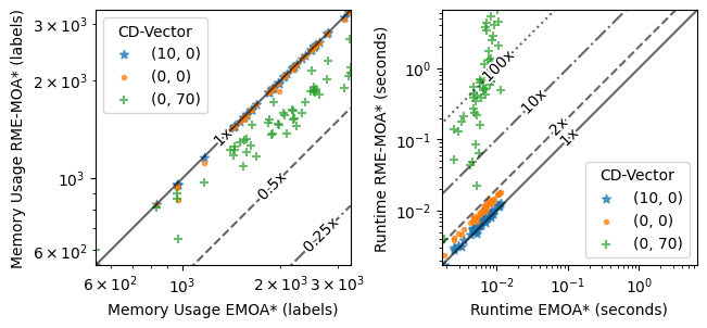
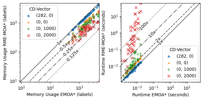
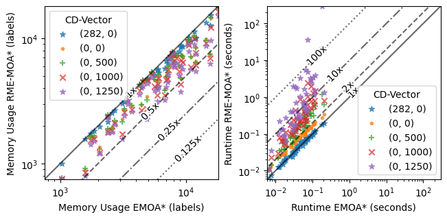
In Fig. 1, we compare the performance of RME-MOA* against EMOA* for - and -connected grids. To note, while , we see negligible improvements in memory usage over EMOA* when the branching factor is small (). However, when (), we see a significant improvement in memory usage (down to 24.23% of the memory usage of EMOA* on average) using RME-MOA* with . Upon further increasing to , RME-MOA* consumes only 5.03% of the memory required of EMOA*. More notably, for , increasing to manages to reduce memory consumption to some degree (75.16% of the memory consumption of EMOA*), where partial expansion alone ( and ) could not. For both branching factors, we see non-negligible increases in runtime (88.36% longer than EMOA* on average for ) when using and , and orders of magnitude worse runtime for large . However, for and (not plotted for visibility), we see substantially improved runtime over (only 8.06% longer than EMOA* on average for ) with nearly the same amount of memory usage (only 7.00% increase in memory usage over on average for ). This implies that, for large branching factor problems, a well-chosen can effectively reduce memory usage (to nearly the limit of the capabilities of RME-MOA*) without sacrificing significant runtime performance. It also shows that, if runtime is not as high a priority as memory efficiency, can be used to further improve memory efficiency, at a heavy runtime cost.
VI-C Robot State Lattice Test
| 20x20 Robot State Lattice Test | |
|---|---|
 |
 |
We then compare RME-MOA* against EMOA* on a mobile robot state lattice, which is similar to the -connected grid test in Sec. VI-B, with the exception that edges between vertices are “differentially constrained”. This means that a robot at vertex can only move immediately to another if is reachable using at least one of a defined set of motion primitives (we refer the reader to [21] for a visualization of these primitives). Each vertex now represents a robot pose, discretized along , , and . Specifically, there exist 8 discrete angles a robot can take on at any () location. This results in a set of approximately 15 distinct motion primitives, corresponding to an average branching factor of 15. We also randomly introduce obstacles at locations with uniform density 0.2. We define 3 practically-oriented cost functions for search on this graph: path length, integrated turning angle over the course of the path, and safety of the path, which we define to be the number of obstacles within an 8-connected vicinity of a vertex.
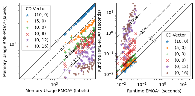
In Fig. 2, we compare the performance of RME-MOA* against EMOA* on this robot state lattice. We see about half the memory consumption using and over EMOA* for (56.98% of EMOA*), and nearly double the runtime (82.20% increase). For , we see even less of a memory improvement (78.99% of EMOA*) but about the same runtime sacrifice (74.51% increase). When is raised until search becomes runtime infeasible, we see a small further improvement for and (30.67% and 67.38% of EMOA*, respectively), while runtime rises again by several orders of magnitude. We attribute this less impressive performance to a smaller branching factor in the robot state lattice () than the grid map (). We also believe that a lack of conflicting objectives may lead only a few promising partial paths to be continually expanded, resulting in a large at each vertex in those paths, and thus a lack of efficacy of the partial expansion technique. This would also explain why RME-MOA* seems to perform worse on higher-dimensional cost functions.
VII Conclusion
This work develops a memory-efficient extension of the recent advanced runtime-efficient MOA* algorithms by generalizing the notion of partial expansion to the multi-objective case, integrating it with the runtime improvements of EMOA*, and fusing this algorithm with PIDMOA* to further improve memory efficiency. Our method, RME-MOA*, balances runtime and memory efficiency via two tunable hyperparameters, which can be set to implement the behavior of EMOA*, PIDMOA*, or some mixture of the two that balances runtime performance with memory efficiency. The results indicate that a properly tuned RME-MOA* is most effective at reducing memory usage for large branching factor problems with minimal runtime increases. RME-MOA* is less effective at reducing memory usage for small branching factor problems, where the ratio between OPEN and CLOSED is very small and partial expansion is less viable. For these problems, more memory efficiency can be gained if necessary by leaning more heavily on PIDMOA* search, at the expense of runtime performance.
Acknowledgments
This material is based upon work supported by the National Science Foundation under Grant No. 2120219 and 2120529. Any opinions, findings, and conclusions or recommendations expressed in this material are those of the author(s) and do not necessarily reflect the views of the National Science Foundation.
References
- [1] E. Erkut, S. A. Tjandra, and V. Verter, “Hazardous materials transportation,” Handbooks in operations research and management science, vol. 14, pp. 539–621, 2007.
- [2] P. Hansen, “Bicriterion path problems,” in Multiple criteria decision making theory and application. Springer, 1980, pp. 109–127.
- [3] F.-J. Pulido, L. Mandow, and J.-L. P. de-la Cruz, “Dimensionality reduction in multiobjective shortest path search,” Computers & Operations Research, vol. 64, pp. 60–70, 2015. [Online]. Available: https://www.sciencedirect.com/science/article/pii/S0305054815001240
- [4] C. Hernández Ulloa, W. Yeoh, J. A. Baier, H. Zhang, L. Suazo, and S. Koenig, “A simple and fast bi-objective search algorithm,” Proceedings of the International Conference on Automated Planning and Scheduling, vol. 30, no. 1, pp. 143–151, Jun. 2020. [Online]. Available: https://ojs.aaai.org/index.php/ICAPS/article/view/6655
- [5] S. Ahmadi, G. Tack, D. D. Harabor, and P. Kilby, “Bi-objective search with bi-directional a*,” in Proceedings of the International Symposium on Combinatorial Search, vol. 12, 2021, pp. 142–144.
- [6] Z. Ren, R. Zhan, S. Rathinam, M. Likhachev, and H. Choset, “Enhanced multi-objective a* using balanced binary search trees,” in Proceedings of the International Symposium on Combinatorial Search, vol. 15, 2022, pp. 162–170.
- [7] H. Zhang, O. Salzman, T. K. S. Kumar, A. Felner, C. Hernández Ulloa, and S. Koenig, “A*pex: Efficient approximate multi-objective search on graphs,” Proceedings of the International Conference on Automated Planning and Scheduling, vol. 32, no. 1, pp. 394–403, Jun. 2022.
- [8] B. Goldin and O. Salzman, “Approximate bi-criteria search by efficient representation of subsets of the pareto-optimal frontier,” in Proceedings of the International Conference on Automated Planning and Scheduling, vol. 31, 2021, pp. 149–158.
- [9] A. Warburton, “Approximation of pareto optima in multiple-objective, shortest-path problems,” Operations research, vol. 35, no. 1, pp. 70–79, 1987.
- [10] M. Pivtoraiko, R. A. Knepper, and A. Kelly, “Differentially constrained mobile robot motion planning in state lattices,” Journal of Field Robotics, vol. 26, no. 3, pp. 308–333, 2009.
- [11] J. Coego, L. Mandow, and J. L. Pérez de la Cruz, “A new approach to iterative deepening multiobjective a*,” in AI*IA 2009: Emergent Perspectives in Artificial Intelligence, R. Serra and R. Cucchiara, Eds. Berlin, Heidelberg: Springer Berlin Heidelberg, 2009, pp. 264–273.
- [12] S. Harikumar and S. Kumar, “Iterative deepening multiobjective a,” Information Processing Letters, vol. 58, no. 1, pp. 11–15, 1996. [Online]. Available: https://www.sciencedirect.com/science/article/pii/0020019096000099
- [13] T. Yoshizumi, T. Miura, and T. Ishida, “A* with partial expansion for large branching factor problems,” in AAAI/IAAI, 2000.
- [14] B. S. Stewart and C. C. White, “Multiobjective a*,” J. ACM, vol. 38, no. 4, p. 775–814, oct 1991. [Online]. Available: https://doi.org/10.1145/115234.115368
- [15] Z. Ren, S. Rathinam, M. Likhachev, and H. Choset, “Multi-objective path-based d* lite,” IEEE Robotics and Automation Letters, vol. 7, no. 2, pp. 3318–3325, 2022.
- [16] E. Q. V. Martins, “On a multicriteria shortest path problem,” European Journal of Operational Research, vol. 16, no. 2, pp. 236–245, 1984.
- [17] P. Sanders and L. Mandow, “Parallel label-setting multi-objective shortest path search,” in 2013 IEEE 27th International Symposium on Parallel and Distributed Processing. IEEE, 2013, pp. 215–224.
- [18] R. E. Korf, “Depth-first iterative-deepening: An optimal admissible tree search,” Artificial Intelligence, vol. 27, no. 1, pp. 97–109, 1985. [Online]. Available: https://www.sciencedirect.com/science/article/pii/0004370285900840
- [19] A. Felner, M. Goldenberg, G. Sharon, R. Stern, T. Beja, N. Sturtevant, J. Schaeffer, and R. Holte, “Partial-expansion a* with selective node generation,” Proceedings of the AAAI Conference on Artificial Intelligence, vol. 26, no. 1, pp. 471–477, Sep. 2021. [Online]. Available: https://ojs.aaai.org/index.php/AAAI/article/view/8137
- [20] R. Stern, N. R. Sturtevant, A. Felner, S. Koenig, H. Ma, T. T. Walker, J. Li, D. Atzmon, L. Cohen, T. K. S. Kumar, E. Boyarski, and R. Barták, “Multi-agent pathfinding: Definitions, variants, and benchmarks,” CoRR, vol. abs/1906.08291, 2019. [Online]. Available: http://arxiv.org/abs/1906.08291
- [21] M. Pivtoraiko, R. A. Knepper, and A. Kelly, “Differentially constrained mobile robot motion planning in state lattices,” Journal of Field Robotics, vol. 26, no. 3, pp. 308–333, 2009. [Online]. Available: https://onlinelibrary.wiley.com/doi/abs/10.1002/rob.20285
- [22] Z. Ren, S. Rathinam, and H. Choset, “A conflict-based search framework for multiobjective multiagent path finding,” IEEE Transactions on Automation Science and Engineering, 2022.