Leveraging Structure for Improved Classification of Grouped Biased Data

Abstract

We consider semi-supervised binary classification for applications in which data points are naturally grouped (e.g., survey responses grouped by state) and the labeled data is biased (e.g., survey respondents are not representative of the population). The groups overlap in the feature space and consequently the input-output patterns are related across the groups. To model the inherent structure in such data, we assume the partition-projected class-conditional invariance across groups, defined in terms of the group-agnostic feature space. We demonstrate that under this assumption, the group carries additional information about the class, over the group-agnostic features, with provably improved area under the ROC curve. Further assuming invariance of partition-projected class-conditional distributions across both labeled and unlabeled data, we derive a semi-supervised algorithm that explicitly leverages the structure to learn an optimal, group-aware, probability-calibrated classifier, despite the bias in the labeled data. Experiments on synthetic and real data demonstrate the efficacy of our algorithm over suitable baselines and ablative models, spanning standard supervised and semi-supervised learning approaches, with and without incorporating the group directly as a feature.

Introduction

Overcoming the problems of learning from biased data is among the most important challenges towards widespread adoption of data-driven technologies (Schwartz et al. 2021). Training machine learning models on biased data may lead to an unacceptable performance deterioration when deployed in the real world, and even more pernicious effects manifest as issues of fairness, when machine learning algorithms systemically lead to worse outcomes for a group of individuals (Mehrabi et al. 2022). However, despite the risks, it is often necessary to train models on biased data as it typically contains signal—in the context of classification, the labeled data may be biased, but it also contains class labels necessary for learning input-output patterns. Correcting for bias is particularly challenging since the mechanisms leading to it are often hidden in the complexities of the data generation process and are difficult to model or evaluate accurately (Storkey 2009). For example, health care data may be biased due to issues of privacy or self-selection, and disease variant databases may be biased towards well-studied or easy-to-study genes and diseases (Stoeger et al. 2018).

A training dataset is biased if the data on which the model is applied cannot be interpreted to be drawn from the same probability distribution. Correcting for bias often relies on assuming some bias model that captures the relationship between biased and unbiased data distributions (Storkey 2009), and then estimating bias correction parameters from the unbiased data (Heckman 1979; Cortes et al. 2008). Thus, bias correction comes under the semi-supervised framework, where unlabeled data is considered to be unbiased and is used to correct the biases arising from training on labeled data.

Covariate shift and label shift are the two most well studied bias assumptions in classification (Storkey 2009). For $x$ and $y$ representing input and output variables, covariate shift assumes that, though the distribution of inputs, $p(x)$, may be different in the labeled and unlabeled data, the distribution of the output at a given input, $p(y|x)$, stays constant. In theory, there is no need for bias correction here, as a nonparametric model trained to learn $p(y|x)$ is not affected by the bias (Rojas 1996). Under label shift, instead of the invariance of $p(y|x)$, the invariance of class-conditionals $p(x|y)$ is assumed. Consequently, the difference in $p(y|x)$ from labeled to unlabeled data is attributed to the change in class priors $p(y)$. Here, the correction of bias relies on an elegant solution of using the model trained on labeled data to estimate the unbiased class priors from unlabeled data (Vucetic and Obradovic 2001; Saerens, Latinne, and Decaestecker 2002).

Though the bias under covariate and label shift can be effectively controlled, the assumptions are too restrictive for many real-world datasets where neither $p(y|x)$ nor $p(x|y)$ are invariant. We therefore introduce a more flexible bias assumption, partition-projected class-conditional invariance (PCC-invariance), that allows both $p(y|x)$ and $p(x|y)$ to vary between labeled and unlabeled data. The assumption relies on the existence of a natural partitioning of the input feature space (Chapelle and Zien 2005), where instead of assuming the invariance of the standard class-conditional distributions, we assume invariance of class-conditional distributions restricted to clusters of the data.

In addition to bias, real-world data often has inherent structure, which may be leveraged for improved learning. Such structure might come from existing features, domain knowledge or additional metadata. For example, census data from different states might be closely related in that input-output patterns learned on Massachusetts can be useful to make predictions on California. General purpose machine learning methods capture such relationships to an extent; however, when such relationships are explicitly modeled by a learner, significant performance gains may be achieved. Furthermore, such structure, when exploited, may also counter the presence of bias. For example, if the labeled data has an underrepresentation of low income households from California, the patterns learned on the low income households from Massachusetts can be exploited.

Here, we consider structured data in domains where objects appear in naturally occurring groups; e.g., individuals grouped by state and variants grouped by gene. Similar to the bias model, our structure assumption is also expressed as PCC-invariance across the groups. The flexibility of this approach allows each group to have a different class-conditional distribution. We show that, under this assumption, a group-aware classifier that incorporates the group information, along with other features, has provably better performance than a group-agnostic classifier. However, the straightforward approach to incorporate the group information as a one-hot encoding is often sub-optimal in practice. Our proposed approach that exploits PCC-invariance across the groups and between labeled and unlabeled data performs better on synthetic and real datasets as compared to the baseline group-aware and group-agnostic classifiers as well as other ablative models.

Problem Formulation

In the context of binary classification, let each object in the population of interest have a representation in the feature space $\mathcal{X}$ and a class label in $\mathcal{Y}=\left\{0,1\right\}$. Additionally, let each object in the population belong to a distinct group, identified by a group index in $\mathcal{G}=\{1,2,\ldots,G\}$. The objects from different groups may overlap in the group-agnostic feature space $\mathcal{X}$; i.e., their $\mathcal{X}$ representations can be arbitrarily close and even coincide. Finally, let $x\in\mathcal{X},y\in\mathcal{Y}$ and $g\in\mathcal{G}$ be the random variables giving the group-agnostic representation, class label and group of an object in the population and $p(x,g,y)$ be the joint distribution of the variables over the population.

CC-Invariance: Under the assumption of class-conditional invariance across groups (CC-invariance), also referred to as label shift in the domain adaptation literature (Garg et al. 2020), the class-conditional distributions of $x$ given $y$ are independent of $g$; i.e.,

$$p(x|y,g)=p(x|y).$$

In other words, the distribution of the input representations coming from the positives ($y=1$) or the negatives ($y=0$) is the same in all groups. However, the groups may differ in the proportion of positives and negatives, so it is possible that $p(y)\neq p(y|g=i)\neq p(y|g=j)$ for some $i\neq j$. Intuitively, the group index does not contain any information about the positive ($p(x|y=1)$) and negative ($p(x|y=0)$) class-conditional distributions, but it still contains information about the class label, as the proportions of positives and negatives differ across the groups. Consequently, in theory, a classifier trained to learn the group-aware posterior, $p(y=1|x,g)$, would be better at predicting the class label.

PCC-Invariance: The CC-invariance assumption might be inadequate for datasets with more complex structure, where the class-conditional distributions differ across groups; i.e., $p(x|y,g=i)\neq p(x|y,g=j)$, for $i\neq j$. If the distributions change arbitrarily across groups, there is no special structure present in the data to be exploited by a learning algorithm. However, many datasets have a clustering structure that can be of use (Chapelle and Zien 2005). We therefore assume the partition-projected class-conditional invariance across groups (PCC-invariance), defined in terms of a partition of $\mathcal{X}$.

Let $\left\{\mathcal{X}_{k}\right\}_{k=1}^{K}$ be a family of subsets of $\mathcal{X}$ that partitions it. We refer to the subsets as clusters. Let $\pi:\mathcal{X}\rightarrow\mathcal{P}=\left\{1,2,\ldots,K\right\}$ be a function that maps each $x\in\mathcal{X}$ to the index of the cluster it belongs to; i.e., for $x\in\mathcal{X}_{k}$, $\pi(x)=k$. Formally, PCC-invariance is defined by the condition

$$p(x|y,g,\pi(x)) =p(x|y,\pi(x)),$$

where $p(x|y,\pi(x))$ is the class-conditional distribution projected on the partition containing $x$. Observe that the CC-invariance is a special case of PCC-invariance, when $K=1$.

For an unambiguous exposition, we refer to the standard class-conditional, $p(x|y)$, simply as the class-conditional and the class-conditional for a group, $p(x|y,g)$, as the group class-conditional. As a consequence of PCC-invariance, each group class-conditional can be expressed as a mixture with the partition-projected class-conditionals as components. The partition proportions in the positives or negatives of the group correspond to the mixing weights. Formally, using $\pi$ also as a random variable giving the cluster index, we have

$$p(x|y,g) =\sum_{k=1}^{K}p(\pi=k|y,g)p(x|y,\pi=k)$$

$$=p(\pi(x)|y,g)p(x|y,\pi(x)).$$

The last expression simplifies the group $g$ class-conditional at $x$ as a product of the class-conditional projected on the partition containing $x$ and the proportion of that partition among the positives or negatives of the group. Note that, though the same components are shared between the groups, the mixing weights may differ from one group to another, which allows the group class-conditionals to be different. Summarizing, PCC-invariance allows group class-conditionals to weigh disjoint regions of $\mathcal{X}$ differently, thereby allowing a more flexible representation than CC-invariance.

Data Assumptions: Next, consider the following setting for the observed data used to train a binary classifier. Let $\mathcal{U}$ be an unlabeled set containing pairs of the form $(x,g)\in\mathcal{X}\times\mathcal{G}$ drawn from $p(x,g)$. Let $\mathcal{L}$ be a labeled set containing triples of the form $(x,g,y)\in\mathcal{X}\times\tilde{\mathcal{G}}\times\mathcal{Y}$, where $\tilde{\mathcal{G}}$ is a group index set, which might be equal to $\mathcal{G}$ or a subset/superset of $\mathcal{G}$ or disjoint from $\mathcal{G}$. Thus, a labeled example may or may not come from the groups that the unlabeled examples belong to. Assume that the labeled triples are drawn from $\tilde{p}\left\lparen x,g,y\right\rparen$, a joint distribution over $\mathcal{X}\times\tilde{\mathcal{G}}\times\mathcal{Y}$. That is, we assume that $\tilde{p}\left\lparen x,g,y\right\rparen$ is a biased version of $p(x,g,y)$. However, similar to $p\left\lparen x,g,y\right\rparen$, $\tilde{p}\left\lparen x,g,y\right\rparen$ follows the PCC-invariance assumption w.r.t. the same clustering function $\pi$; i.e.,

$$\tilde{p}(x|y,g,\pi(x)) =\tilde{p}(x|y,\pi(x)).$$

Furthermore, though $\tilde{p}\left\lparen x,g,y\right\rparen$ and $p\left\lparen x,g,y\right\rparen$ are different distributions, we assume them to have equal partition-projected class-conditionals; i.e.,

$$\tilde{p}(x|y,\pi(x)) =p(x|y,\pi(x)).$$

This assumption is critical for the input-output patterns learned on a labeled data partition to be optimal on the corresponding unlabeled partition, in spite of the bias in the class-conditionals and the group class-conditionals; i.e., $p(x|y)\neq\tilde{p}(x|y)$ and $p(x|y,g)\neq\tilde{p}(x|y,g)$. Figure 1 gives an example in which the aforementioned assumptions hold.

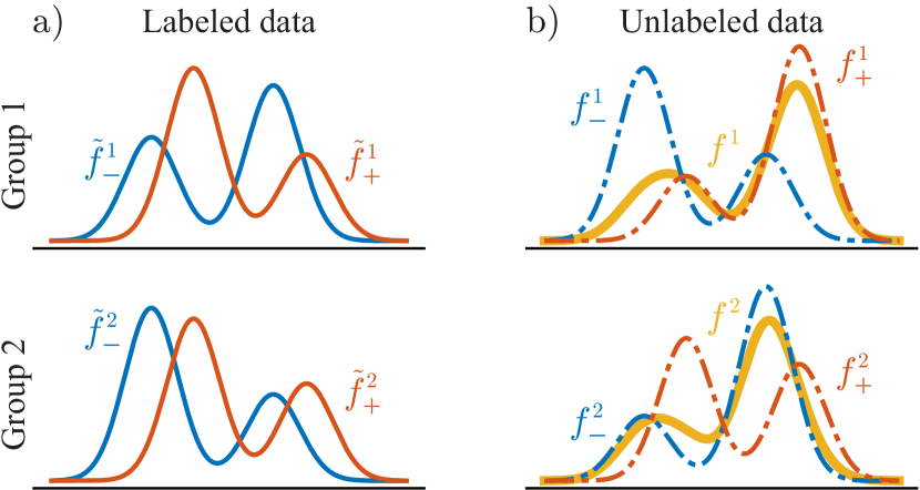
Figure 1: Illustration of the structure and bias considered in this work. (a) Group class-conditionals for the labeled data. $\tilde{f}^{g}_{+}(x)=\tilde{p}(x|y=1,g)$ and $\tilde{f}^{g}_{-}(x)=\tilde{p}(x|y=0,g)$ are the positive and negative class-conditionals for group $g$, respectively. The solid curves indicate that we observe data from the labeled group class-conditionals. (b) Group class-conditionals and marginals for the unlabeled data. $f^{g}_{+}(x)=p(x|y=1,g)$ and $f^{g}_{-}(x)=p(x|y=0,g)$ are the positive and negative class-conditionals for group $g$, respectively. $f^{g}(x)=p(x|g)$ is the group $g$ marginal over $x$. The dashed-dotted curves indicate that we do not observe data from the unlabeled group class-conditionals, but we do observe data from the group marginals. Notice the difference in the class-conditionals across groups and between the labeled and unlabeled data. Also notice that all the positive (negative) group class-conditionals are mixtures sharing the same components, but differing w.r.t. their mixing weights. Additionally, labeled data class priors are generally different from unlabeled data class priors.

Problem Statement: In this paper, we are motivated by the problem of learning a classifier from $\mathcal{L}$ and $\mathcal{U}$ for optimally predicting class labels for $(x,g)$ drawn from $p(x,g)$. Consider the following two types of classifiers: (1) a group-agnostic classifier that only uses the representation $x$ to separate the positives from the negatives; i.e., a classifier with a score function of the form $s:\mathcal{X}\rightarrow\mathbb{R}$, and (2) a group-aware classifier that uses both the representation $x$ and group index $g$; i.e., a classifier with a score function of the form $\bar{s}:\mathcal{X}\times\mathcal{G}\rightarrow\mathbb{R}$. In theory, a group-aware classifier should be at least as good as the group-agnostic one and better than a group-agnostic classifier if the groups carry additional information about the class. In practice, however, a group-aware classifier trained on finite data could be suboptimal since more complex models have a higher propensity to overfit. Thus, it is important to theoretically ascertain if the groups carry additional information about the class and only train a group-aware classifier if that is indeed the case. Furthermore, in that case, it is not obvious how to best incorporate the group information when training a group-aware classifier.

The straightforward approach of encoding the group as a one-hot feature does not explicitly leverage the PCC-invariance. Can the groups be incorporated in a manner in which the assumptions are directly leveraged to train a group-aware classifier with improved empirical performance? Additionally, since the labeled data has biased class-conditionals, a classifier trained on the labeled data is likely to be sub-optimal. Can the unlabeled data be exploited by the algorithm to correct for the biases, giving an optimal classification? Our work seeks to answer these questions.

Contributions

This paper reveals the following:

1. Knowing the group of an object indeed carries additional information about the class, over that carried by the representation. Further, the improvement in classification brought about by the group can be theoretically quantified in terms of data distribution parameters.

2. Our novel semi-supervised algorithm is capable of incorporating the groups in a manner that directly exploits the PCC-invariance assumption to learn a group-aware classifier that is demonstrably better than the group-aware classifier based on one-hot encoding of groups, the group-agnostic classifier, and other ablative models on synthetic and real-world data.

3. The posterior probability, $p(y=1|x,g)$, can be expressed in terms of quantities that can be estimated from labeled and unlabeled data.

4. Despite labeled data bias, our semi-supervised algorithm can learn an optimal classifier under the data assumptions by estimating unbiased distribution parameters on the unlabeled data and using them to correct for the bias.

Theoretical Results

In this section, we prove that under PCC-invariance, the groups indeed carry additional information about the class relative to that carried by the group-agnostic features (Theorem 1). The result is shown in terms of the area under the ROC curve (AUC) improvements brought about by an optimal group-aware classifier, given by the posterior $\bar{\rho}(x,g)=p(y=1|x,g)$, over an optimal group-agnostic classifier, given by $\rho(x)=p(y=1|x)$. Additionally, we show that $\bar{\rho}(x,g)$ can be expressed in terms of distribution parameters that can be estimated from labeled and unlabeled data (Theorem 2). The theorem directly informs our algorithm for practical estimation of $\bar{\rho}(x,g)$.

Let $f_{+}(x)=p(x|y=1)$ and $f_{-}(x)=p(x|y=0)$ be the class-conditional densities for the positive and negative class. Let $\bar{f}_{+}(x,g)=p(x,g|y=1)$ and $\bar{f}_{-}(x,g)=p(x,g|y=0)$ denote the joint density function of the $x$ and $g$ given the class. Theoretically, the AUC of a group-agnostic score function, $s(x)$, can be expressed as

$$\textup{AUC}(s) =P\left\lparen\tau_{s}(x_{1},x_{0})>1\right\rparen+\nicefrac{{1}}{{2}}P\left\lparen\tau_{s}(x_{1},x_{0})=1\right\rparen,$$

where $x_{1}\sim f_{+}$, $x_{0}\sim f_{-}$ and $\tau_{s}(x_{1},x_{0})=\nicefrac{{s(x_{1})}}{{s(x_{0})}}$. Similarly, the AUC of a group-aware score function, $\bar{s}(x,g)$, can be expressed as

$$\textup{AUC}(\bar{s}) =P\left\lparen\tau_{\bar{s}}(x_{1},g_{1},x_{0},g_{0})>1\right\rparen$$

$$\quad+\nicefrac{{1}}{{2}}P\left\lparen\tau_{\bar{s}}(x_{1},g_{1},x_{0},g_{0})=1\right\rparen,$$

where $\tau_{\bar{s}}(x_{1},g_{1},x_{0},g_{0})=\nicefrac{{\bar{s}(x_{1},g_{1})}}{{\bar{s}(x_{0},g_{0})}}$, $(x_{1},g_{1})\sim\bar{f}_{+}$ and $(x_{0},g_{0})\sim\bar{f}_{-}$.

Next, consider two group-agnostic score functions: (1) posterior-based, $\rho(x)=p(y=1|x)$, and (2) density ratio-based, $r(x)=\nicefrac{{f_{+}(x)}}{{f_{-}(x)}}$. It can be shown that a density ratio-based score function or any score function that ranks the data points in the same order achieves the highest AUC (Uematsu and Lee 2011). Thus $r$ achieves the highest AUC among all score functions defined on $\mathcal{X}$ and so does $\rho$ since both functions rank the points in $\mathcal{X}$ in the same order; i.e., $\textup{AUC}(r)=\textup{AUC}(\rho).$

Further, consider the group-aware posterior as the score function, $\bar{\rho}(x,g)=p(y=1|x,g)$. Similar to the discussion above, $\bar{\rho}$ achieves the highest AUC among all score functions defined on $\mathcal{X}\times\mathcal{G}$. In Theorem 1, we show that incorporating the group information improves classification as $\textup{AUC}(\bar{\rho})$ is greater than or equal to $\textup{AUC}(\rho)$. The increase in $\textup{AUC}(\bar{\rho})$ is expressed in terms of random variables $\tau_{r}^{10}=\nicefrac{{r(x_{1})}}{{r(x_{0})}}$, $\tau_{r}^{01}=\nicefrac{{r(x_{0})}}{{r(x_{1})}}$, $\omega^{10}=\omega\left\lparen g_{1},\pi(x_{1}),g_{0},\pi(x_{0})\right\rparen$ and $\omega^{01}=\omega\left\lparen g_{0},\pi(x_{0}),g_{1},\pi(x_{1})\right\rparen$, where $\omega(g,k,h,j)=\nicefrac{{\textup{OR}\left\lparen\alpha_{k}^{g},\alpha_{k}\right\rparen}}{{\textup{OR}\left\lparen\alpha_{j}^{h},\alpha_{j}\right\rparen}}$, $\alpha_{k}^{g}=p(y=1|g,\pi=k)$ is the proportion of positives in partition $k$ for group $g$ and $\alpha_{k}=p(y=1|\pi=k)$ is the proportion of positives in partition $k$ overall, across all groups; $\textup{OR}(p,q)=\frac{\nicefrac{{p}}{{(1-p)}}}{\nicefrac{{q}}{{(1-q)}}}$ is the odds ratio between probabilities $p$ and $q$. When $p=q=0$ or $p=q=1$, $\textup{OR}(p,q)$ should be evaluated as $1$.

Notice that the right-hand side in Theorem 1 is non-negative because the indicator and the Dirac delta functions ensure that $\omega^{10}<\tau_{r}^{01}$. Furthermore, it is strictly positive when $\omega^{10}<\tau_{r}^{01}\leq 1$ with non-zero probability. Note that $\tau^{10}$ and $\tau^{01}$ depend on feature representations of a pair of positive and negative points, but not on their groups, whereas $\omega^{10}$ and $\omega^{01}$ depend on their groups and the feature representations, however, at a level of granularity, captured by their cluster memberships. Intuitively, the largest increase in AUC is attained when the features in $\mathcal{X}$ have no predictive power ($f_{+}=f_{-}$); i.e., $\textup{AUC}(\rho)=0.5$ and $\forall x\in\mathcal{X}$, $r(x)=1$. In this case, $\tau^{10}=1$ with probability $1$. Now, if all group-cluster pairs are pure ($\forall k\in\mathcal{P}$ and $g\in\mathcal{G}$, $\alpha_{k}^{g}$ is equal to $1$ or $0$), then $\omega^{01}=0$ with probability $1$ and the first and second expectations evaluate to $0.5$ and $0$, respectively, giving $\textup{AUC}(\bar{\rho})=1$. In general, a large overlap between $f_{+}$ and $f_{-}$ gives small values of $\textup{AUC}(\rho)$ and thus a more significant increase in AUC can be expected theoretically, provided the group within a cluster tend to be purer than the cluster. In practice, however, a large overlap would lead to a large variance in estimating group-cluster pair positive proportions (Methods) and, consequently, the expected increase in AUC of the group-aware classifier might be compromised. In an extreme case, when $f_{+}=f_{-}$, the group-cluster pair positive proportions are unidentifiable and cannot be estimated.

Theorem 1.

(Proof in Appendix) Let $\mathbb{E}$ denote the expectation over $(x_{1},g_{1}){\sim}\bar{f}_{+}$ and $(x_{0},g_{0}){\sim}\bar{f}_{-}$; $\omega^{10}=\omega(g_{1},\pi(x_{1}),g_{0},\pi(x_{0}))$, $\omega^{01}=\nicefrac{{1}}{{\omega^{10}}}$, $\tau_{r}^{10}=\tau_{r}(x_{1},x_{0})$ and $\tau_{r}^{01}=\nicefrac{{1}}{{\tau_{r}^{10}}}$; $\mathbb{I}_{a}^{b}\left\lparen\cdot\right\rparen$ be the indicator function for the open interval $(a,b)$ and $\delta_{a}\left\lparen\cdot\right\rparen$ be the Dirac delta function, evaluating to $1$ at $a\in\real$ and to $0$ otherwise. It follows that

$$\textup{AUC}(\bar{\rho})-\textup{AUC}(\rho)=\mathbb{E}\left[\delta_{0}\left\lparen\omega^{01}\right\rparen\left\lparen\mathbb{I}_{0}^{1}\left\lparen\tau_{r}^{10}\right\rparen{+}\nicefrac{{1}}{{2}}\delta_{1}\left\lparen\tau_{r}^{10}\right\rparen\right\rparen\right]$$

$$\quad+\mathbb{E}\left[\mathbb{I}_{0}^{1}\left\lparen\omega^{10}\right\rparen\left\lparen\mathbb{I}_{\omega^{10}}^{1}\left\lparen\tau_{r}^{01}\right\rparen{+}\nicefrac{{1}}{{2}}\delta_{1}\left\lparen\tau_{r}^{01}\right\rparen\right\rparen\left\lparen\nicefrac{{\tau_{r}^{01}}}{{\omega^{10}}}{-}1\right\rparen\right].$$

Theorem 2.

(Proof in Appendix) For $\tilde{\rho}(x)=\tilde{p}(y=1|x)$, $\tilde{\alpha}_{k}=\tilde{p}(y=1|\pi=k)$ and $\alpha^{g}_{k}=p(y=1|g,\pi=k)$,

$$\bar{\rho}(x,g)=\left\lparen 1+\textup{OR}\left\lparen\tilde{\alpha}_{\pi(x)},\alpha^{g}_{\pi(x)}\right\rparen\frac{1-\tilde{\rho}(x)}{\tilde{\rho}(x)}\right\rparen^{-1}.$$

Methods

In this section, we introduce our main semi-supervised learning algorithm for training an optimal, bias-corrected, group-aware classifier from $\mathcal{L}$ and $\mathcal{U}$. To this end, we estimate the probability-calibrated score function $\bar{\rho}(x,g)$ by explicitly leveraging PCC-invariance and the additional assumptions relating the labeled and unlabeled data distribution described in the Problem Formulation section. The algorithm is given by the following steps.

1. Cluster: Apply k-means clustering to $\mathcal{L}\ \cup\ \mathcal{U}$, the combined pool of labeled and unlabeled data to partition $\mathcal{X}$ into $K$ clusters, $\left\{\mathcal{X}_{k}\right\}_{k=1}^{K}$. Use the silhouette coefficient (de Amorim and Hennig 2015) to determine $K$.

2. Estimate $\bm{\tilde{\rho}(x)=\tilde{p}(y=1|x)}$: Estimate the labeled data posterior by training a probabilistic classifier on $\mathcal{L}$ using group-agnostic features only. Note that a separate classifier may be trained on each labeled cluster to estimate $\tilde{\rho}(x)$, since $\tilde{p}(y=1|x)=\tilde{p}(y=1|x,\pi(x))$.

3. Estimate $\bm{\tilde{\alpha}_{k}=\tilde{p}(y=1|\pi=k)}$: Estimate the proportion of positives in each cluster in $\mathcal{L}$ by counting the positives in the cluster and dividing by the size of the cluster.

4. Estimate $\bm{{\alpha}^{g}_{k}=p(y=1|g,\pi=k)}$: Estimate the proportion of positives in each group and cluster pair from $\mathcal{U}$ by applying one of the approaches used for domain-adaptation under label shift; see next Section.

5. Estimate $\bm{\bar{\rho}(x,g)=p(y=1|x,g)}$: Estimate the group-aware posterior by applying the formula derived in Theorem 2, using the estimates of $\tilde{\rho}(x)$, $\tilde{\alpha}_{\pi(x)}$ and $\alpha^{g}_{\pi(x)}$, computed in the previous steps.

Except for the estimation of ${\alpha}^{g}_{k}$ in step 4, all other steps are straightforward to implement. We estimate ${\alpha}^{g}_{k}$ using techniques from domain-adaptation under label shift as follows.

Estimating Class Proportions under Label Shift

The key insight for estimation of ${\alpha}^{g}_{k}$ is that, when restricted to a single cluster, the labeled data and the unlabeled data form an instance of single-source and multi-target domain-adaptation under label shift (same as CC-invariance). Let $\mathcal{L}_{k}=\left\{(x,y)|x\in\mathcal{X}_{k},(x,g,y)\in\mathcal{L}\right\}$ be the subset of $\mathcal{L}$ containing points from the $k$^th cluster only. Let $\mathcal{U}_{k}^{g}=\left\{x|x\in\mathcal{X}_{k},(x,g)\in\mathcal{U}\right\}$ be the subset of $\mathcal{U}$ containing points from the $k$^th cluster and $g$^th group only. $\mathcal{L}_{k}$ serves as the source domain and $\left\{\mathcal{U}_{k}^{g}\right\}_{g=1}^{G}$ serves as the $G$ target-domains. Since PCC-invariance across groups and the data assumptions imply $p(x|y,g,\pi(x))=p(x|y,\pi(x))=\tilde{p}(x|y,\pi(x))$, the underlying distributions of positives (negatives) in $\mathcal{L}_{k}$ and $\mathcal{U}_{k}^{g}$ are equal. The marginal distributions of $x$ corresponding to $\mathcal{L}_{k}$ and $\mathcal{U}_{k}^{g}$ only differ in terms of the class proportions. Thus, the label-shift assumptions are satisfied between $\mathcal{L}_{k}$ and $\mathcal{U}_{k}^{g}$, which make estimation of ${\alpha}^{g}_{k}$ feasible.

The two state-of-the-art approaches to estimate the target domain class proportions under label-shift are:

• Maximum Likelihood Label Shift (MLLS): an Expectation Maximization (EM) based maximum-likelihood estimator of the class proportions that relies on a calibrated probabilistic classifier trained on the source domain (Saerens, Latinne, and Decaestecker 2002).

• Black Box Shift Estimation (BBSE): a moment-matching based class proportion estimator that works with calibrated or uncalibrated classifier trained on the source domain (Lipton, Wang, and Smola 2018).

We decided to use MLLS to estimate ${\alpha}^{g}_{k}$, since it has been shown to outperform BBSE empirically (Alexandari, Kundaje, and Shrikumar 2020). Formally, ${\alpha}^{g}_{k}$ is estimated in an EM framework by iteratively updating it until convergence. Starting with an initial estimate $\hat{\alpha}^{g}_{k}\left<0\right>=\nicefrac{{1}}{{\left|\mathcal{U}^{g}_{k}\right|}}\sum_{x\in\mathcal{U}^{g}_{k}}\check{\rho}(x)$, where $\check{\rho}(x)$ is the group-agnostic posterior estimated from $\mathcal{L}$ in step 2, it is updated in iteration $t$ as

$$\hat{\alpha}^{g}_{k}\left<t+1\right>\leftarrow\frac{1}{\left|\mathcal{U}^{g}_{k}\right|}\sum_{x\in\mathcal{U}^{g}_{k}}\left\lparen 1+\textup{OR}\left\lparen\check{\alpha}_{k},\hat{\alpha}^{g}_{k}\left<t\right>\right\rparen\frac{1-\check{\rho}(x)}{\check{\rho}(x)}\right\rparen^{-1}$$

where $\check{\alpha}_{k}$ is the proportion of positives in $\mathcal{L}_{k}$ computed in step 3.

Experiments and Empirical Results

Datasets

The method was evaluated on synthetic and real-world data in two settings: (1) setting 1, where the class-conditionals are identical across groups and between labeled and unlabeled data, and (2) setting 2, where the class-conditionals vary, but the partition-projected class-conditionals are invariant (PCC-invariance assumption holds).

Synthetic Data: We generated synthetic data from Gaussian mixtures. The positive and negative examples in cluster $k$ were drawn from a pair of $d$-dimensional Gaussian components, N$(\mu^{+}_{k},\Sigma^{+}_{k})$ and N$(\mu^{-}_{k},\Sigma^{-}_{k})$, respectively. Their location and shape parameters were obtained by random perturbations such that the overlap between the pair corresponded to a within-cluster AUC in the range $[0.75,0.95]$. The component pair for each cluster was generated one after the other, further ensuring that they do not overlap significantly with the component pairs already generated.

Once the component pairs for all clusters were determined, the data for setting 1 and 2 were generated as follows. Each dataset was generated with 100 groups. The sizes of group $g$ in the labeled ($\left|\mathcal{L}^{g}\right|$) and unlabeled ($\left|\mathcal{U}^{g}\right|$) data were determined by drawing a random number from N$(1000,100^{2})$ and N$(10000,1000^{2})$, respectively, and rounding to the closest integer. The data dimension ($d$) and the number of clusters ($K$) were picked from $\{1,2,4,8\}$ and $\{1,4,16,64\}$, respectively, in all pairs of combinations. Next,

• for setting 1, the cluster proportions, $\left[\gamma_{k}\right]_{k=1}^{K}$, were sampled from the $K$-dimensional symmetric Dirichlet$(K,2)$. The proportion of positives in cluster $k$ ($\alpha_{k}$) was sampled from Uniform$(0.01,0.99)$. Then, $\gamma_{k}\alpha_{k}\left|\mathcal{L}^{g}\right|$ and $\gamma_{k}\alpha_{k}\left|\mathcal{U}^{g}\right|$ examples (rounded to the closest integer) were sampled from N$(\mu^{+}_{k},\Sigma^{+}_{k})$ as the labeled and unlabeled positives for group $g$, respectively. Similarly, $\gamma_{k}(1-\alpha_{k})\left|\mathcal{L}^{g}\right|$ and $\gamma_{k}(1-\alpha_{k})\left|\mathcal{U}^{g}\right|$ examples were sampled from N$(\mu^{-}_{k},\Sigma^{-}_{k})$ as the labeled and unlabeled negatives for group $g$, respectively.

• for setting 2, the group $g$ cluster proportions for the labeled ($\left[\tilde{\gamma}_{k}^{g}\right]_{k=1}^{K}$) and unlabeled ($\left[\gamma_{k}^{g}\right]_{k=1}^{K}$) data were sampled from the $K$-dimensional symmetric Dirichlet$(K,2)$. The proportion of positives in cluster $k$ for group $g$ in labeled ($\tilde{\alpha}_{k}^{g}$) and unlabeled ($\alpha_{k}^{g}$) data were sampled from Uniform$(0.01,0.99)$. Then, $\tilde{\gamma}^{g}_{k}\tilde{\alpha}^{g}_{k}\left|\mathcal{L}^{g}\right|$ and $\gamma^{g}_{k}\alpha^{g}_{k}\left|\mathcal{U}^{g}\right|$ examples (rounded to the closest integer) were sampled from N$(\mu^{+}_{k},\Sigma^{+}_{k})$ as the labeled and unlabeled positives for group $g$, respectively. Similarly, $\tilde{\gamma}^{g}_{k}(1-\tilde{\alpha}^{g}_{k})\left|\mathcal{L}^{g}\right|$ and $\gamma^{g}_{k}(1-\alpha^{g}_{k})\left|\mathcal{U}^{g}\right|$ examples were sampled from N$(\mu^{-}_{k},\Sigma^{-}_{k})$ as the labeled and unlabeled negatives for group $g$, respectively

Real-World Data: Three binary classification datasets, generated from the Folktables American Community Survey (ACS) data (Ding et al. 2021), were used for evaluation: Income, Income Poverty Ratio (IPR), and Employment (Table 3, Appendix). Additional high-dimensional embeddings data can also be found in the Appendix, available on arXiv.

For each dataset, labeled ($\mathcal{L}$) and unlabeled ($\mathcal{U}$) samples for the two settings were generated from the pool of available labeled examples $\mathcal{D}$. State was used as the group variable in the ACS datasets. The sets of all group $g$ examples in $\mathcal{D}$ were first equally divided into labeled ($L^{g}$) and unlabeled ($U^{g}$) pools. The final labeled ($\mathcal{L}^{g}$) and unlabeled ($\mathcal{U}^{g}$) sets for group $g$ were generated by resampling with replacement from $L^{g}$ and $U^{g}$. To this end, $\mathcal{D}$ was first partitioned into $K$ clusters by running mini-batch k-means with batch size 4096, where $K$ was chosen from $\{1,2,4,8\}$, to maximize the silhouette coefficient on a random sample of 25,000 examples.

To create a setting 1 dataset, first, $\left[\gamma_{k}\right]_{k=1}^{K}$ and $\alpha_{k}$ were sampled similarly as for the synthetic datasets. Then, $\gamma_{k}\alpha_{k}|L^{g}|$ and $\gamma_{k}\alpha_{k}|U^{g}|$ examples sampled from the positives in $L^{g}$ and $U^{g}$, lying in cluster $k$, were added to $\mathcal{L}^{g}$ and $\mathcal{U}^{g}$, respectively. Similarly, $\gamma_{k}(1-\alpha_{k})|L^{g}|$ and $\gamma_{k}(1-\alpha_{k})|U^{g}|$ examples sampled from the negatives in $L^{g}$ and $U^{g}$, lying in cluster $k$, were also added to $\mathcal{L}^{g}$ and $\mathcal{U}^{g}$.

To create a setting 2 dataset, first, $\left[\tilde{\gamma}^{g}_{k}\right]_{k=1}^{K}$, $\left[\gamma^{g}_{k}\right]_{k=1}^{K}$, $\tilde{\alpha}^{g}_{k}$ $\alpha^{g}_{k}$ were sampled similarly as for the synthetic datasets. Then $\tilde{\gamma}^{g}_{k}\tilde{\alpha}^{g}_{k}|L^{g}|$ and $\gamma^{g}_{k}\alpha^{g}_{k}|U^{g}|$ examples sampled from the positives in $L^{g}$ and $U^{g}$, lying in cluster $k$, were added to $\mathcal{L}^{g}$ and $\mathcal{U}^{g}$, respectively. Similarly, $\tilde{\gamma}^{g}_{k}(1-\tilde{\alpha}^{g}_{k})|L^{g}|$ and $\gamma^{g}_{k}(1-\alpha^{g}_{k})|U^{g}|$ examples sampled from the negatives in $L^{g}$ and $U^{g}$, lying in cluster $k$, were also added to $\mathcal{L}^{g}$ and $\mathcal{U}^{g}$.

Experimental Protocol

Experiments were run at least 10 times for each dataset, repeating the data generation process each time. The performance of each method was measured using AUC on a held-out set of 20% of the groups of unique examples in $\mathcal{U}$, averaged over all repetitions.

A held-out validation set was constructed by randomly removing 20% of groups of unique examples in $\mathcal{L}$. Our method fits a mini-batch k-means model to $\mathcal{L}\cup\mathcal{U}$ with batch size 4096, to estimate the clustering used to generate the data. $K\in\{1,2,4,8\}$ is selected to maximize the silhouette coefficient estimated on a random batch of 25,000 examples. A random forest of 500 decision trees with maximum depth of 10 was fit to each cluster in the labeled training data, splitting on the gini criterion. All classifiers were calibrated by Platt’s scaling (Platt 1999) using a held-out validation set. The MLLS algorithm was run for 100 iterations to estimate the unlabeled group-cluster class priors ${\alpha}^{g}_{k}$.

The method was compared to five baseline methods: (1) Global, where a single classifier is trained on the labeled examples, (2) Group-Aware Global, where the group-agnostic feature representation of each example is concatenated with a one-hot encoded vector of that example’s group, (3) Cluster Global, where a separate classifier is trained on each cluster in the labeled data, (4) Label Shift, where a single classifier is trained on the labeled examples and then adjusted to the estimated class prior of each group’s unlabeled distribution, and (5) CORAL, a domain adaptation method where a separate classifier is trained for each group, aligning the second order statistics of the labeled examples to those of the group’s unlabeled examples (Sun, Feng, and Saenko 2016). Note that Label Shift is a special case of our method ($K=1$). The same model training, selection, and calibration procedures, as described above, were used in all baseline methods.

Comparative Experiments on Synthetic Data

Figure 2 shows the distribution of AUCs calculated on the test data relative to the global classifier, with the AUCs for each dimensionality-cluster pair averaged over all iterations. The left sub-figure shows that our method maintains performance even when applied on datasets in which examples are all drawn from the same distribution. The right sub-figure shows that our method leads to substantial improvement in AUC when examples are drawn from distributions with the assumed bias model. Figure 3 shows the effects of $d$ and $K$ on the relative performance of our method. Our method maintains strong performance when applied to datasets with both high dimensionality and many clusters.

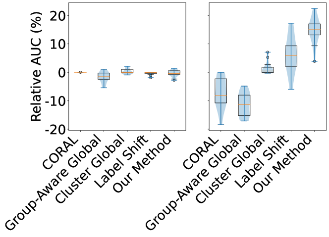
Figure 2: Distribution of average AUCs, calculated on the held-out test set, relative to the AUC of Global on synthetic datasets. Left: setting 1, Right: setting 2.

.

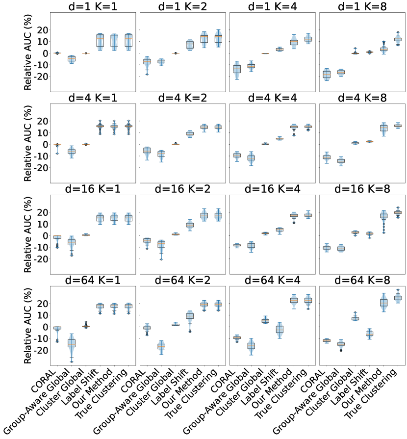
Figure 3: Distribution of AUCs, calculated on the held-out test set, relative to the AUC of Global on synthetic datasets in setting 2 separated by $d$ and $K$.

Comparative Experiments on Real-World Data

Tables 1 and 2 list the AUCs calculated on the test set, averaged over all repetitions, for real-world datasets generated in settings 1 and 2, respectively. Table 1 shows that our method maintains comparable performance to that of Global despite the data lacking the bias our method aims to address. The experiments summarized in Table 2 demonstrate the theoretical performance improvements our method can realize when presented with real-world biased data.

Method	Income	Employment	IPR
CORAL	0.865	0.883	0.792
Global	0.879	0.903	0.825
Group-Aware Global	0.870	0.897	0.812
Cluster Global	0.879	0.903	0.828
Label Shift	0.873	0.900	0.812
Our Method	0.874	0.898	0.812
True Clustering	0.873	0.900	0.812

Table 1: Average AUC calculated on the held-out test set for real-world datasets in setting 1.

Method	Income	Employment	IPR
CORAL	0.853	0.851	0.760
Global	0.870	0.897	0.816
Group-Aware Global	0.846	0.865	0.768
Cluster Global	0.871	0.898	0.820
Label Shift	0.876	0.904	0.831
Our Method	0.884	0.916	0.850
True Clustering	0.900	0.927	0.862

Table 2: Average AUC calculated on the held-out test set for real-world datasets in setting 2.

Effects of Clustering

Because our method fits a clustering model on the resampled dataset, not the original dataset that is used to find the clustering during data generation, it is possible that our method does not recover the true clustering used to generate the observed samples. These estimated and true clusterings can differ in the cluster centers and number of clusters. To analyze the effect the quality of the clustering has on classification performance, we compare our method’s performance to that of our method when given access to the true clustering used to generate the data. Figure 3 shows the extent to which the performance of our method is affected by estimating the clustering on resampled data in the experiments. The performance degrades with the increasing number of clusters, becoming noticeable at $K=8$. Table 2 shows that additional improvements in performance could be made with access to the true clustering of the data in the case of real-world datasets with bias.

Related Work

Since the early work by Heckman (1979), the problem of learning from biased data has been extensively studied under sample selection bias, dataset shift, transfer learning and domain adaptation (Peng et al. 2003; Zadrozny 2004; Dudik, Schapire, and Phillips 2005; Ben-David et al. 2006; Huang et al. 2006; Cortes et al. 2008; Storkey 2009; Daumé III 2009; Pan and Yang 2010; Hsieh, Niu, and Sugiyama 2019; Jain et al. 2020; Garg et al. 2020; De Paolis Kaluza, Jain, and Radivojac 2023). Most recently, learning predictive models in settings where the training and test distributions differ has been studied extensively in the literature of domain adaptation (Kouw and Loog 2019; Garg et al. 2020). Our problem relates to this literature in that it can be reformulated as an instance of multi-target unsupervised domain adaptation by considering the collection of all labeled examples as the source domain and the unlabeled examples from each group as a distinct target domain with a novel assumption placed on the distributions of these domains.

Several methods, including MLLS (Saerens, Latinne, and Decaestecker 2002) and BBSE (Lipton, Wang, and Smola 2018), have been developed to correct for label shift, which we refer to as CC-invariance, for single-target unsupervised domain adaptation and have been shown to relate to the distribution-matching methods (Garg et al. 2020). While not explored in these works, under the CC-invariance assumption only, it would be straightforward to apply these distribution matching approaches in isolation to each group to correct for differences in class priors. In a less rigid PCC-invariance assumption shared across the labeled and unlabeled groups, it is assumed that both prior and class-conditional distributions differ across groups, yet the bias correction remains practical by generalizing the methodology developed to address CC-invariance.

While we are unaware of any previous work proposing the PCC-invariance assumption, there exists prior work on covariate shift that assumes different class-conditional distributions across groups. In the context of regression, flexibility has been given to class-conditional distributions across training and test sets by introducing a latent variable $r$ and assuming $p_{\textrm{train}}(x,y|r)=p_{\textrm{test}}(x,y|r)$ and $p_{\textrm{train}}(r)\neq p_{\textrm{test}}(r)$ (Storkey and Sugiyama 2006).

Conclusions

The partition-projected class-conditional invariance (PCC-invariance) assumption, introduced in this paper, is a flexible means of modeling bias and structure in binary classification problems with grouped data. In contrast to the existing bias models, it allows both the posterior ($p(y|x)$) and the class-conditional ($p(x|y)$) in the labeled data to be biased and yet facilitates theoretically sound bias correction with the aid of unbiased unlabeled data. Moreover, as a model to capture structure between groups, under PCC-invariance  a group-aware classifier achieves a provably improved AUC over a group-agnostic classifier.

By directly exploiting PCC-invariance, our semi-supervised algorithm is an effective approach for bias correction and exploiting the group structure present in the data, as demonstrated by improved performance over group-agnostic and group-aware classifiers on real and synthetic data. Furthermore, the approach is robust to the absence of bias and structure in the data as demonstrated by the experiments. Lastly, the approach has a desirable property of learning a probability-calibrated classifier.

Appendix A Theorems and Proofs

Theorem 1.

Let $p(x,g,y)$ be a joint distribution on $\mathcal{X}\times\mathcal{G}\times\mathcal{Y}$ satisfying PCC-invariance w.r.t. the partitioning function $\pi:\mathcal{X}\rightarrow\mathcal{P}$ as described in Problem Formulation. For $\rho(x)=p(y=1|x)$ and $\bar{\rho}(x,g)=p(y=1|x,g)$,

$$\textup{AUC}(\bar{\rho}) =\textup{AUC}\left\lparen\rho\right\rparen+\mathbb{E}\left[\mathbb{I}_{(0,1)}\left\lparen\omega^{10}\right\rparen\left\lparen\mathbb{I}_{\left\lparen\omega^{10},1\right\rparen}\left\lparen\tau_{r}^{01}\right\rparen+\frac{1}{2}\delta_{1}\left\lparen\tau_{r}^{01}\right\rparen\right\rparen\left\lparen\frac{\tau_{r}^{01}}{\omega^{10}}-1\right\rparen\right]+\mathbb{E}\left[\left\lparen\mathbb{I}_{\left\lparen 0,1\right\rparen}\left\lparen\tau_{r}^{10}\right\rparen+\frac{1}{2}\delta_{1}\left\lparen\tau_{r}^{10}\right\rparen\right\rparen\times\delta_{0}\left\lparen\omega^{01}\right\rparen\right]$$

where the expectation is taken over $(x_{1},g_{1}){\sim}\bar{f}_{+}$ and $(x_{0},g_{0}){\sim}\bar{f}_{-}$; $\omega^{10}=\omega(g_{1},\pi(x_{1}),g_{0},\pi(x_{0}))$ and $\omega^{01}=\nicefrac{{1}}{{\omega^{10}}}$; $\tau_{r}^{10}=\tau_{r}(x_{1},x_{0})$ and $\tau_{r}^{01}=\nicefrac{{1}}{{\tau_{r}^{10}}}$; $\mathbb{I}_{A}\left\lparen\cdot\right\rparen$ is the indicator function for set $A$ and $\delta_{a}\left\lparen\cdot\right\rparen$ be the Dirac delta function, evaluating to $1$ at $a\in\real$ and to $0$ otherwise.

Proof.

First we derive the following expression for the group-aware posterior $\bar{\rho}(x,g)=p(y=1|x,g)$ can be expressed as

$$\bar{\rho}(x,g) =p\left\lparen y=1|x,g,\pi(x)\right\rparen$$

$$=\frac{p\left\lparen y=1|g,\pi(x)\right\rparen p\left\lparen x|y=1,g,\pi(x)\right\rparen}{p\left\lparen x|g,\pi(x)\right\rparen}$$

$$=\frac{p\left\lparen y=1|g,\pi(x)\right\rparen p\left\lparen x|y=1,\pi(x)\right\rparen}{p\left\lparen x|g,\pi(x)\right\rparen}$$

$$=\frac{p\left\lparen y=1|g,\pi(x)\right\rparen p\left\lparen x|y=1,\pi(x)\right\rparen}{p\left\lparen y=1|g,\pi(x)\right\rparen p\left\lparen x|y=1,\pi(x)\right\rparen+p\left\lparen y=0|g,\pi(x)\right\rparen p\left\lparen x|y=0,\pi(x)\right\rparen}$$

$$=\frac{\alpha^{g}_{\pi(x)}f^{\prime}_{+}(x)}{\alpha^{g}_{\pi(x)}f^{\prime}_{+}(x)+\left\lparen 1-\alpha^{g}_{\pi(x)}\right\rparen f^{\prime}_{-}(x)},$$ (1)

where $\alpha^{g}_{k}=p(y=1|g,\pi=k)$ is the proportion of positives in group $g$ examples coming from partition $k$; $f^{\prime}_{+}(x)=p(x|y=1,\pi(x))$ and $f^{\prime}_{-}(x)=p(x|y=0,\pi(x))$ are the class-conditionals projected on the partition containing $x$. Next, we derive the following expression for $f^{\prime}_{+}(x)$.

$$f^{\prime}_{+}(x) =p(x|y=1,\pi(x))$$

$$=\frac{p(x,\pi(x)|y=1)}{p(\pi(x)|y=1)}$$

$$=\frac{f_{+}(x)}{\frac{p(\pi(x))p(y=1|\pi(x))}{p(y=1)}}$$

$$=\frac{\alpha f_{+}(x)}{\alpha_{\pi(x)}\gamma_{\pi(x)}},$$ (2)

where $\alpha=p(y=1)$, the proportion of positives in the entire distribution; $\alpha_{k}=p(y=1|\pi=k)$, the proportion of positives in the partition $k$; $\gamma_{k}=p\left\lparen\pi=k\right\rparen$, the proportion of examples lying in partition $k$ from the entire distribution. Note that if $f_{+}(x)=0$ on the entire partition $\pi(x)$, containing point $x$, $\alpha_{\pi(x)}$ is equal to 0 as well, which leads to $0/0$ on the right hand side. Since $f^{\prime}_{+}(x)=0$ on the entire partition $\pi(x)$ in this case, we consider the RHS to be equal to 0. Similarly,

$$f^{\prime}_{-}(x) =\frac{(1-\alpha)f_{-}(x)}{\left\lparen 1-\alpha_{\pi(x)}\right\rparen\gamma_{\pi(x)}}.$$ (3)

Again note that if $f_{-}(x)=0$ on the entire partition $\pi(x)$, containing point $x$, $1-\alpha_{\pi(x)}$ is equal to 0 as well, which leads to $0/0$ on the right hand side. Since $f^{\prime}_{-}(x)=0$ on the entire partition $\pi(x)$ in this case, we consider the RHS to be equal to 0.

Next, we derive the following expression from Eq. 1.

$$\frac{\bar{\rho}(x,g)}{1-\bar{\rho}(x,g)} =\frac{\alpha^{g}_{\pi(x)}f^{\prime}_{+}(x)}{\left\lparen 1-\alpha^{g}_{\pi(x)}\right\rparen f^{\prime}_{-}(x)}$$

$$=\frac{\frac{\alpha\alpha^{g}_{\pi(x)}}{\alpha_{\pi(x)}\gamma_{\pi(x)}}f_{+}(x)}{\frac{(1-\alpha)\left\lparen 1-\alpha^{g}_{\pi(x)}\right\rparen}{\left\lparen 1-\alpha_{\pi(x)}\right\rparen\gamma_{\pi(x)}}f_{-}(x)}$$ (from Eq. 2 and 3)

$$=\frac{\alpha}{1-\alpha}\textup{OR}\left\lparen\alpha^{g}_{\pi(x)},\alpha_{\pi(x)}\right\rparen r(x),$$ (4)

where $r(x)=\nicefrac{{f_{+}(x)}}{{f_{-}(x)}}$; $\textup{OR}(p,q)=\frac{\nicefrac{{p}}{{(1-p)}}}{\nicefrac{{q}}{{(1-q)}}}$ is the odds ratio between probabilities $p$ and $q$. Defined as such, $\textup{OR}(p,q)$ is not well-defined when $p=q=0$ or $p=q=1$. We extend the definition in the two cases as $\textup{OR}(p,q)=1$. Due to this extension, Eq. 1 still holds true when $\alpha_{\pi(x)}$ is equal to $0$ or $1$. Precisely, $\alpha_{\pi(x)}=0$ means that partition $\pi(x)$ does not contain any positives and consequently $r(x)=0$, $\bar{\rho}(x,g)=0$ and $\alpha^{g}_{\pi(x)}=0$ for any $g\in\mathcal{G}$. Thus both RHS and LHS are equal. Similarly, $\alpha_{\pi(x)}=1$ means that partition $\pi(x)$ does not contain any negatives and consequently $r(x)=\infty$, $\bar{\rho}(x,g)=1$ and $\alpha^{g}_{\pi(x)}=1$ for any $g\in\mathcal{G}$. Thus both RHS and LHS are equal.

Next, for inputs $x_{0},x_{1}\in\mathcal{X}$ and groups $g_{0},g_{1}\in\mathcal{G}$,

$$\bar{\rho}(x_{1},g_{1})>\bar{\rho}(x_{0},g_{0}) \Leftrightarrow\frac{\bar{\rho}(x_{1},g_{1})}{1-\bar{\rho}(x_{1},g_{1})}>\frac{\bar{\rho}(x_{0},g_{0})}{1-\bar{\rho}(x_{0},g_{0})}$$

$$\Leftrightarrow\textup{OR}\left\lparen\alpha^{g_{1}}_{\pi(x_{1})},\alpha_{\pi(x_{1})}\right\rparen r(x_{1})>\textup{OR}\left\lparen\alpha^{g_{0}}_{\pi(x_{0})},\alpha_{\pi(x_{0})}\right\rparen r(x_{0})$$

$$\Leftrightarrow\tau_{r}(x_{1},x_{0})>\omega\left\lparen g_{0},\pi(x_{0}),g_{1},\pi(x_{1})\right\rparen,$$

where $\tau_{r}(x_{1},x_{0})=\nicefrac{{r(x_{1})}}{{r(x_{0})}}$ and $\omega(g,k,h,j)=\frac{\textup{OR}\left\lparen\alpha_{k}^{g},\alpha_{k}\right\rparen}{\textup{OR}\left\lparen\alpha_{j}^{h},\alpha_{j}\right\rparen}$. Similarly,

$$\bar{\rho}(x_{1},g_{1})=\bar{\rho}(x_{0},g_{0}) \Leftrightarrow\tau_{r}(x_{1},x_{0})=\omega\left\lparen g_{0},\pi(x_{0}),g_{1},\pi(x_{1})\right\rparen.$$

Note that for a positive $x\in\mathcal{X}$ belonging to group $g\in\mathcal{G}$, $\alpha^{g}_{\pi(x)}\neq 0$ and $\alpha_{\pi(x)}\neq 0$. Thus $\textup{OR}\left\lparen\alpha^{g}_{\pi(x)},\alpha_{\pi(x)}\right\rparen\neq 0$. Similarly for a negative $x\in\mathcal{X}$ belonging to group $g\in\mathcal{G}$ $\alpha^{g}_{\pi(x)}\neq 1$ and $\alpha_{\pi(x)}\neq 1$. Thus $\textup{OR}\left\lparen\alpha^{g}_{\pi(x)},\alpha_{\pi(x)}\right\rparen\neq\infty$. Now, if $x_{1}$ is positive and $x_{0}$ is negative, $\omega\left\lparen g_{0},\pi(x_{0}),g_{1},\pi(x_{1})\right\rparen$ is well-defined, finite and could potentially take $0$ value. In contrast, if $x_{0}$ is positive and $x_{1}$ is negative, $\omega\left\lparen g_{0},\pi(x_{0}),g_{1},\pi(x_{1})\right\rparen$ is well-defined and non zero, but not necessarily finite.

Let $P_{10}$ and $\mathbb{E}_{10}$ denote the probabilities and expectations computed with $(x_{1},g_{1})\sim\bar{f}_{+}(x,g)=p(x,g|y=1)$ and $(x_{0},g_{0})\sim\bar{f}_{-}(x,g)=p(x,g|y=0)$. Similarly, $P_{01}$ and $\mathbb{E}_{01}$ denote the probabilities and expectations computed with $(x_{0},g_{0})\sim\bar{f}_{+}(x,g)$ and $(x_{1},g_{1})\sim\bar{f}_{-}(x,g)$. Further, let $\omega^{10}=\omega(g_{1},\pi(x_{1}),g_{0},\pi(x_{0}))$, $\omega^{01}=\omega(g_{0},\pi(x_{0}),g_{1},\pi(x_{1}))$, $\tau_{r}^{10}=\tau_{r}(x_{1},x_{0})$ and $\tau_{r}^{01}=\tau_{r}(x_{0},x_{1})$. Note that $\omega^{01}=\nicefrac{{1}}{{\omega^{10}}}$ and $\tau_{r}^{01}=\nicefrac{{1}}{{\tau_{r}^{10}}}$ Now,

$$\textup{AUC}\left\lparen\bar{\rho}\right\rparen =P_{10}\left\lparen\bar{\rho}(x_{1},b_{1})>\bar{\rho}(x_{0},b_{0})\right\rparen+\frac{1}{2}P_{10}\left\lparen\bar{\rho}(x_{1},b_{1})=\bar{\rho}(x_{0},b_{0})\right\rparen$$

$$=P_{10}\left\lparen\tau_{r}^{10}>\omega^{01}\right\rparen+\frac{1}{2}P_{10}\left\lparen\tau_{r}^{10}=\omega^{01}\right\rparen$$

$$=P_{10}\left\lparen\tau_{r}^{10}>\omega^{01}\ \&\ \omega^{01}\geq 1\right\rparen+P_{10}\left\lparen\tau_{r}^{10}>\omega^{01}\ \&\ \omega^{01}<1\right\rparen+\frac{1}{2}P_{10}\left\lparen\tau_{r}^{10}=\omega^{01}\right\rparen$$

$$=P_{10}\left\lparen\tau_{r}^{10}>1\ \&\ \omega^{01}\geq 1\right\rparen-P_{10}\left\lparen 1<\tau_{r}^{10}\leq\omega^{01}\ \&\ \omega^{01}>1\right\rparen$$

$$\quad+P_{10}\left\lparen\tau_{r}^{10}>1\ \&\ \omega^{01}<1\right\rparen+P_{10}\left\lparen 1\geq\tau_{r}^{10}>\omega^{01}\ \&\ \omega^{01}<1\right\rparen+\frac{1}{2}P_{10}\left\lparen\tau_{r}^{10}=\omega^{01}\right\rparen$$

$$=P_{10}\left\lparen\tau_{r}^{10}>1\right\rparen+P_{10}\left\lparen 1\geq\tau_{r}^{10}>\omega^{01}\ \&\ \omega^{01}<1\right\rparen-P_{10}\left\lparen 1<\tau_{r}^{10}\leq\omega^{01}\ \&\ \omega^{01}>1\right\rparen$$

$$\quad+\frac{1}{2}P_{10}\left\lparen\tau_{r}^{10}=1\right\rparen+\frac{1}{2}P_{10}\left\lparen\tau_{r}^{10}=\omega^{01}\right\rparen-\frac{1}{2}P_{10}\left\lparen\tau_{r}^{10}=1\right\rparen$$

$$=\textup{AUC}\left\lparen\rho\right\rparen+P_{10}\left\lparen 1>\tau_{r}^{10}>\omega^{01}\ \&\ \omega^{01}<1\right\rparen+P_{10}\left\lparen\tau_{r}^{10}=1\ \&\ \omega^{01}<1\right\rparen$$

$$\quad-P_{10}\left\lparen 1<\tau_{r}^{10}<\omega^{01}\ \&\ \omega^{01}>1\right\rparen-P_{10}\left\lparen\tau_{r}^{10}=\omega^{01}\ \&\ \omega^{01}>1\right\rparen \rho \tau_{r}$$ (because AUC() = AUC())

$$\quad+\frac{1}{2}P_{10}\left\lparen\tau_{r}^{10}=\omega^{01}\ \&\ \omega^{01}\neq 1\right\rparen-\frac{1}{2}P_{10}\left\lparen\tau_{r}^{10}=1\ \&\ \omega^{01}\neq 1\right\rparen$$

$$=\textup{AUC}\left\lparen\rho\right\rparen+P_{10}\left\lparen 1>\tau_{r}^{10}>\omega^{01}\ \&\ \omega^{01}<1\right\rparen-P_{10}\left\lparen 1<\tau_{r}^{10}<\omega^{01}\ \&\ \omega^{01}>1\right\rparen$$

$$\quad+\frac{1}{2}\left\lparen P_{10}\left\lparen\tau_{r}^{10}=\omega^{01}\ \&\ \omega^{01}<1\right\rparen-P_{10}\left\lparen\tau_{r}^{10}=\omega^{01}\ \&\ \omega^{01}>1\right\rparen\right\rparen$$

$$\quad+\frac{1}{2}\left\lparen P_{10}\left\lparen\tau_{r}^{10}=1\ \&\ \omega^{01}<1\right\rparen-P_{10}\left\lparen\tau_{r}^{10}=1\ \&\ \omega^{01}>1\right\rparen\right\rparen$$

As demonstrated earlier, since $x_{1}$ is positive and $x_{0}$ is negative under $P_{10}$, $\omega^{01}$ is well-defined and finite. Furthermore it is non-negative by definition. In other words $0\leq\omega^{01}<\infty$ with probability $1$ under $P_{10}$. Thus

$$\textup{AUC}\left\lparen\bar{\rho}\right\rparen =\textup{AUC}\left\lparen\rho\right\rparen+P_{10}\left\lparen 1>\tau_{r}^{10}>\omega^{01}\ \&\ 0\leq\omega^{01}<1\right\rparen-P_{10}\left\lparen 1<\tau_{r}^{10}<\omega^{01}\ \&\ \infty>\omega^{01}>1\right\rparen$$

$$\quad+\frac{1}{2}\left\lparen P_{10}\left\lparen\tau_{r}^{10}=\omega^{01}\ \&\ 0\leq\omega^{01}<1\right\rparen-P_{10}\left\lparen\tau_{r}^{10}=\omega^{01}\ \&\ \infty>\omega^{01}>1\right\rparen\right\rparen$$

$$\quad+\frac{1}{2}\left\lparen P_{10}\left\lparen\tau_{r}^{10}=1\ \&\ 0\leq\omega^{01}<1\right\rparen-P_{10}\left\lparen\tau_{r}^{10}=1\ \&\ \infty>\omega^{01}>1\right\rparen\right\rparen$$

$$=\textup{AUC}\left\lparen\rho\right\rparen+P_{10}\left\lparen 1>\tau_{r}^{10}>\omega^{01}\ \&\ 0<\omega^{01}<1\right\rparen-P_{10}\left\lparen 1<\tau_{r}^{10}<\omega^{01}\ \&\ \infty>\omega^{01}>1\right\rparen$$

$$\quad+\frac{1}{2}\left\lparen P_{10}\left\lparen\tau_{r}^{10}=\omega^{01}\ \&\ 0<\omega^{01}<1\right\rparen-P_{10}\left\lparen\tau_{r}^{10}=\omega^{01}\ \&\ \infty>\omega^{01}>1\right\rparen\right\rparen$$

$$\quad+\frac{1}{2}\left\lparen P_{10}\left\lparen\tau_{r}^{10}=1\ \&\ 0<\omega^{01}<1\right\rparen-P_{10}\left\lparen\tau_{r}^{10}=1\ \&\ \infty>\omega^{01}>1\right\rparen\right\rparen$$

$$\quad+P_{10}\left\lparen 1>\tau_{r}^{10}>0\ \&\ \omega^{01}=0\right\rparen+\frac{1}{2}P_{10}\left\lparen\tau_{r}^{10}=0\ \&\ \omega^{01}=0\right\rparen+\frac{1}{2}P_{10}\left\lparen\tau_{r}^{10}=1\ \&\ \omega^{01}=0\right\rparen$$

$$=\textup{AUC}\left\lparen\rho\right\rparen+P_{10}\left\lparen 1>\tau_{r}^{10}>\omega^{01}\ \&\ 0<\omega^{01}<1\right\rparen-P_{10}\left\lparen 1<\tau_{r}^{10}<\omega^{01}\ \&\ \infty>\omega^{01}>1\right\rparen$$

$$\quad+\frac{1}{2}\left\lparen P_{10}\left\lparen\tau_{r}^{10}=\omega^{01}\ \&\ 0<\omega^{01}<1\right\rparen-P_{10}\left\lparen\tau_{r}^{10}=\omega^{01}\ \&\ \infty>\omega^{01}>1\right\rparen\right\rparen$$

$$\quad+\frac{1}{2}\left\lparen P_{10}\left\lparen\tau_{r}^{10}=1\ \&\ 0<\omega^{01}<1\right\rparen-P_{10}\left\lparen\tau_{r}^{10}=1\ \&\ \infty>\omega^{01}>1\right\rparen\right\rparen$$

$$\quad+P_{10}\left\lparen 1>\tau_{r}^{10}>0\ \&\ \omega^{01}=0\right\rparen+\frac{1}{2}P_{10}\left\lparen\tau_{r}^{10}=1\ \&\ \omega^{01}=0\right\rparen \tau_{r}^{10}>0 P_{10}$$ (because with probability 1 under )

Now converting probabilities to expectations,

$$\textup{AUC}\left\lparen\bar{\rho}\right\rparen =\textup{AUC}\left\lparen\rho\right\rparen+\mathbb{E}_{10}\left[\mathbb{I}_{\left\lparen\omega^{01},1\right\rparen}\left\lparen\tau_{r}^{10}\right\rparen\times\mathbb{I}_{(0,1)}\left\lparen\omega^{01}\right\rparen\right]-\mathbb{E}_{10}\left[\mathbb{I}_{\left\lparen 1,\omega^{01}\right\rparen}\left\lparen\tau_{r}^{10}\right\rparen\times\mathbb{I}_{(1,\infty)}\left\lparen\omega^{01}\right\rparen\right]$$

$$\quad+\frac{1}{2}\left\lparen\mathbb{E}_{10}\left[\delta_{\omega^{01}}\left\lparen\tau_{r}^{10}\right\rparen\times\mathbb{I}_{(0,1)}\left\lparen\omega^{01}\right\rparen\right]-\mathbb{E}_{10}\left[\delta_{\omega^{01}}\left\lparen\tau_{r}^{10}\right\rparen\times\mathbb{I}_{(1,\infty)}\left\lparen\omega^{01}\right\rparen\right]\right\rparen$$

$$\quad+\frac{1}{2}\left\lparen\mathbb{E}_{10}\left[\delta_{1}\left\lparen\tau_{r}^{10}\right\rparen\times\mathbb{I}_{(0,1)}\left\lparen\omega^{01}\right\rparen\right]-\mathbb{E}_{10}\left[\delta_{1}\left\lparen\tau_{r}^{10}\right\rparen\times\mathbb{I}_{(1,\infty)}\left\lparen\omega^{01}\right\rparen\right]\right\rparen$$

$$\quad+\mathbb{E}_{10}\left[\mathbb{I}_{\left\lparen 0,1\right\rparen}\left\lparen\tau_{r}^{10}\right\rparen\times\delta_{0}\left\lparen\omega^{01}\right\rparen\right]+\frac{1}{2}\mathbb{E}_{10}\left\lparen\delta_{1}\left\lparen\tau_{r}^{10}\right\rparen\times\delta_{0}\left\lparen\omega^{01}\right\rparen\right\rparen$$ (5)

To simplify the expressions further, we first derive the following expression

$$\frac{\bar{f}_{+}(x_{1},g_{1})\bar{f}_{-}(x_{0},g_{0})}{\bar{f}_{+}(x_{0},g_{0})\bar{f}_{-}(x_{1},g_{1})} =\frac{p(x_{1},g_{1}|y_{1}=1)p(x_{0},g_{0}|y_{0}=0)}{p(x_{1},g_{1}|y_{1}=0)p(x_{0},g_{0}|y_{0}=1)}$$

$$=\frac{\frac{p(y_{1}=1|x_{1},g_{1})}{p(y_{1}=1)}\frac{p(y_{0}=0|x_{0},g_{0})}{p(y_{0}=1)}}{\frac{p(y_{1}=0|x_{1},g_{1})}{p(y_{1}=0)}\frac{p(y_{0}=1|x_{0},g_{0})}{p(y_{0}=1)}}$$

$$=\frac{\bar{\rho}(x_{1},g_{1})\left\lparen 1-\bar{\rho}(x_{0},g_{0})\right\rparen}{\left\lparen 1-\bar{\rho}(x_{1},g_{1})\right\rparen\bar{\rho}(x_{0},g_{0})}$$

$$=\frac{\textup{OR}\left\lparen\alpha^{g_{1}}_{\pi(x_{1})},\alpha_{\pi(x_{1})}\right\rparen r(x_{1})}{\textup{OR}\left\lparen\alpha^{g_{0}}_{\pi(x_{0})},\alpha_{\pi(x_{0})}\right\rparen r(x_{0})}$$

$$=\frac{\tau_{r}(x_{1},x_{0})}{\omega(g_{0},\pi(x_{0}),g_{1},\pi(x_{1}))}.$$ (6)

Using the expression above, $\mathbb{E}_{10}$ expectation of a finite valued function $\lambda(x_{1},g_{1},x_{0},g_{0})$, that vanishes to $0$ when $\tau_{r}(x_{1},x_{0})=\infty$ or $\omega(g_{0},\pi(x_{0}),g_{1},\pi(x_{1}))=0$, can be expressed as an $\mathbb{E}_{01}$ expectation as follows.

$$\mathbb{E}_{10}\left[\lambda(x_{1},g_{1},x_{0},g_{0})\right] =\sum_{(g_{1},g_{0})\in\mathcal{G}^{2}}\int_{(x_{1},x_{0})\in\mathcal{X}^{2}}\lambda(x_{1},g_{1},x_{0},g_{0})\bar{f}_{+}(x_{1},g_{1})\bar{f}_{-}(x_{0},g_{0})dx_{1}dx_{0}$$

$$=\sum_{(g_{1},g_{0})\in\mathcal{G}^{2}}\int_{(x_{1},x_{0})\in\mathcal{X}^{2}}\lambda(x_{1},g_{1},x_{0},g_{0})\frac{\bar{f}_{+}(x_{1},g_{1})\bar{f}_{-}(x_{0},g_{0})}{\bar{f}_{+}(x_{0},g_{0})\bar{f}_{-}(x_{1},g_{1})}\bar{f}_{+}(x_{0},g_{0})\bar{f}_{-}(x_{1},g_{1})dx_{1}dx_{0}$$ (under certain conditions given below)

$$=\sum_{(g_{1},g_{0})\in\mathcal{G}^{2}}\int_{(x_{1},x_{0})\in\mathcal{X}^{2}}\lambda(x_{1},g_{1},x_{0},g_{0})\frac{\tau_{r}(x_{1},x_{0})}{\omega(g_{0},\pi(x_{0}),g_{1},\pi(x_{1}))}\bar{f}_{+}(x_{0},g_{0})\bar{f}_{-}(x_{1},g_{1})dx_{1}dx_{0}$$

$$=\mathbb{E}_{01}\left[\lambda(x_{1},g_{1},x_{0},g_{0})\frac{\tau_{r}(x_{1},x_{0})}{\omega(g_{0},\pi(x_{0}),g_{1},\pi(x_{1}))}\right].$$

The above derivation is valid if

$$\bar{f}_{+}(x_{0},g_{0})\bar{f}_{-}(x_{1},g_{1})=0\Rightarrow\lambda(x_{1},g_{1},x_{0},g_{0})\bar{f}_{+}(x_{1},g_{1})\bar{f}_{-}(x_{0},g_{0})=0.$$

Next we show that if $\lambda(x_{1},g_{1},x_{0},g_{0})$ vanishes to $0$ when $\tau_{r}(x_{1},x_{0})=\infty$ or $\omega(g_{0},\pi(x_{0}),g_{1},\pi(x_{1}))=0$, then the above implication is indeed satisfied. We present a proof by contradiction. Suppose $\bar{f}_{+}(x_{0},g_{0})\bar{f}_{-}(x_{1},g_{1})=0$, but $\lambda(x_{1},g_{1},x_{0},g_{0})\bar{f}_{+}(x_{1},g_{1})\bar{f}_{-}(x_{0},g_{0})\neq 0.$ Thus from Eq. 6, $\frac{\tau_{r}(x_{1},x_{0})}{\omega(g_{0},\pi(x_{0}),g_{1},\pi(x_{1}))}=\infty$, which is only possible if $\tau_{r}(x_{1},x_{0})=\infty$ or $\omega(g_{0},\pi(x_{0}),g_{1},\pi(x_{1}))=0$. Thus $\lambda(x_{1},g_{1},x_{0},g_{0})=0$ and consequently $\lambda(x_{1},g_{1},x_{0},g_{0})\bar{f}_{+}(x_{1},g_{1})\bar{f}_{-}(x_{0},g_{0})=0$, which leads to the contradiction.

Note that $\mathbb{E}_{10}$ expectation can also be converted to $\mathbb{E}_{01}$ expectation by swapping the variables; i.e., $\mathbb{E}_{10}\left[\lambda(x_{1},g_{1},x_{0},g_{0})\right]=\mathbb{E}_{01}\left[\lambda(x_{0},g_{0},x_{1},g_{1})\right]$. Now, converting the $\mathbb{E}_{10}$ expectations on the first three lines of the RHS of Eq. 5 to $\mathbb{E}_{01}$ expectations, using the two rules derived above,

$$\textup{AUC}\left\lparen\bar{\rho}\right\rparen =\textup{AUC}\left\lparen\rho\right\rparen+\mathbb{E}_{01}\left[\mathbb{I}_{\left\lparen\omega^{01},1\right\rparen}\left\lparen\tau_{r}^{10}\right\rparen\times\mathbb{I}_{(0,1)}\left\lparen\omega^{01}\right\rparen\times\nicefrac{{\tau_{r}^{10}}}{{\omega^{01}}}\right]-\mathbb{E}_{01}\left[\mathbb{I}_{\left\lparen 1,\omega^{10}\right\rparen}\left\lparen\tau_{r}^{01}\right\rparen\times\mathbb{I}_{\left\lparen 1,\infty\right\rparen}\left\lparen\omega^{10}\right\rparen\right]$$

$$\quad+\frac{1}{2}\left\lparen\mathbb{E}_{01}\left[\delta_{\omega^{01}}\left\lparen\tau_{r}^{10}\right\rparen\times\mathbb{I}_{(0,1)}\left\lparen\omega^{01}\right\rparen\times\nicefrac{{\tau_{r}^{10}}}{{\omega^{01}}}\right]-\mathbb{E}_{01}\left[\delta_{\omega^{10}}\left\lparen\tau_{r}^{01}\right\rparen\times\mathbb{I}_{(1,\infty)}\left\lparen\omega^{10}\right\rparen\right]\right\rparen$$

$$\quad+\frac{1}{2}\left\lparen\mathbb{E}_{01}\left[\delta_{1}\left\lparen\tau_{r}^{10}\right\rparen\times\mathbb{I}_{(0,1)}\left\lparen\omega^{01}\right\rparen\times\nicefrac{{\tau_{r}^{10}}}{{\omega^{01}}}\right]-\mathbb{E}_{01}\left[\delta_{1}\left\lparen\tau_{r}^{01}\right\rparen\times\mathbb{I}_{(1,\infty)}\left\lparen\omega^{10}\right\rparen\right]\right\rparen$$

$$\quad+\mathbb{E}_{10}\left[\mathbb{I}_{\left\lparen 0,1\right\rparen}\left\lparen\tau_{r}^{10}\right\rparen\times\delta_{0}\left\lparen\omega^{01}\right\rparen\right]+\frac{1}{2}\mathbb{E}_{10}\left\lparen\delta_{1}\left\lparen\tau_{r}^{10}\right\rparen\times\delta_{0}\left\lparen\omega^{01}\right\rparen\right\rparen$$

Next, observing that $\tau_{r}^{01}=\nicefrac{{1}}{{\tau_{r}^{10}}}$ and $\omega^{10}=\nicefrac{{1}}{{\omega^{01}}}$,

$$\textup{AUC}\left\lparen\bar{\rho}\right\rparen =\textup{AUC}\left\lparen\rho\right\rparen+\mathbb{E}_{01}\left[\mathbb{I}_{\left\lparen\omega^{01},1\right\rparen}\left\lparen\tau_{r}^{10}\right\rparen\times\mathbb{I}_{(0,1)}\left\lparen\omega^{01}\right\rparen\times\nicefrac{{\tau_{r}^{10}}}{{\omega^{01}}}\right]-\mathbb{E}_{01}\left[\mathbb{I}_{\left\lparen\omega^{01},1\right\rparen}\left\lparen\tau_{r}^{10}\right\rparen\times\mathbb{I}_{(0,1)}\left\lparen\omega^{01}\right\rparen\right]$$

$$\quad+\frac{1}{2}\left\lparen\mathbb{E}_{01}\left[\delta_{\omega^{01}}\left\lparen\tau_{r}^{10}\right\rparen\times\mathbb{I}_{(0,1)}\left\lparen\omega^{01}\right\rparen\times\nicefrac{{\tau_{r}^{10}}}{{\omega^{01}}}\right]-\mathbb{E}_{01}\left[\delta_{\omega^{01}}\left\lparen\tau_{r}^{10}\right\rparen\times\mathbb{I}_{(0,1)}\left\lparen\omega^{01}\right\rparen\right]\right\rparen$$

$$\quad+\frac{1}{2}\left\lparen\mathbb{E}_{01}\left[\delta_{1}\left\lparen\tau_{r}^{10}\right\rparen\times\mathbb{I}_{(0,1)}\left\lparen\omega^{01}\right\rparen\times\nicefrac{{\tau_{r}^{10}}}{{\omega^{01}}}\right]-\mathbb{E}_{01}\left[\delta_{1}\left\lparen\tau_{r}^{10}\right\rparen\times\mathbb{I}_{(0,1)}\left\lparen\omega^{01}\right\rparen\right]\right\rparen$$

$$\quad+\mathbb{E}_{10}\left[\mathbb{I}_{\left\lparen 0,1\right\rparen}\left\lparen\tau_{r}^{10}\right\rparen\times\delta_{0}\left\lparen\omega^{01}\right\rparen\right]+\frac{1}{2}\mathbb{E}_{10}\left\lparen\delta_{1}\left\lparen\tau_{r}^{10}\right\rparen\times\delta_{0}\left\lparen\omega^{01}\right\rparen\right\rparen$$

$$=\textup{AUC}\left\lparen\rho\right\rparen+\mathbb{E}_{01}\left[\left\lparen\mathbb{I}_{\left\lparen\omega^{01},1\right\rparen}\left\lparen\tau_{r}^{10}\right\rparen+\frac{1}{2}\delta_{\omega^{01}}\left\lparen\tau_{r}^{10}\right\rparen+\frac{1}{2}\delta_{1}\left\lparen\tau_{r}^{10}\right\rparen\right\rparen\times\mathbb{I}_{(0,1)}\left\lparen\omega^{01}\right\rparen\times\left\lparen\nicefrac{{\tau_{r}^{10}}}{{\omega^{01}}}-1\right\rparen\right]$$

$$\quad+\mathbb{E}_{10}\left[\left\lparen\mathbb{I}_{\left\lparen 0,1\right\rparen}\left\lparen\tau_{r}^{10}\right\rparen+\frac{1}{2}\delta_{1}\left\lparen\tau_{r}^{10}\right\rparen\right\rparen\times\delta_{0}\left\lparen\omega^{01}\right\rparen\right]$$

$$=\textup{AUC}\left\lparen\rho\right\rparen+\mathbb{E}_{01}\left[\left\lparen\mathbb{I}_{\left\lparen\omega^{01},1\right\rparen}\left\lparen\tau_{r}^{10}\right\rparen+\frac{1}{2}\delta_{1}\left\lparen\tau_{r}^{10}\right\rparen\right\rparen\times\mathbb{I}_{(0,1)}\left\lparen\omega^{01}\right\rparen\times\left\lparen\nicefrac{{\tau_{r}^{10}}}{{\omega^{01}}}-1\right\rparen\right]$$

$$\quad+\mathbb{E}_{10}\left[\left\lparen\mathbb{I}_{\left\lparen 0,1\right\rparen}\left\lparen\tau_{r}^{10}\right\rparen+\frac{1}{2}\delta_{1}\left\lparen\tau_{r}^{10}\right\rparen\right\rparen\times\delta_{0}\left\lparen\omega^{01}\right\rparen\right] \delta_{\omega^{01}}\left\lparen\tau_{r}^{10}\right\rparen=1\Rightarrow\nicefrac{{\tau_{r}^{10}}}{{\omega^{01}}}=1$$ (because )

Finally, again converting $\mathbb{E}_{01}$ expectation in line 1 to $\mathbb{E}_{10}$ by swapping the variables,

$$\textup{AUC}\left\lparen\bar{\rho}\right\rparen =\textup{AUC}\left\lparen\rho\right\rparen+\mathbb{E}_{10}\left[\left\lparen\mathbb{I}_{\left\lparen\omega^{10},1\right\rparen}\left\lparen\tau_{r}^{01}\right\rparen+\frac{1}{2}\delta_{1}\left\lparen\tau_{r}^{01}\right\rparen\right\rparen\times\mathbb{I}_{(0,1)}\left\lparen\omega^{10}\right\rparen\times\left\lparen\nicefrac{{\tau_{r}^{01}}}{{\omega^{10}}}-1\right\rparen\right]$$

$$\quad+\mathbb{E}_{10}\left[\left\lparen\mathbb{I}_{\left\lparen 0,1\right\rparen}\left\lparen\tau_{r}^{10}\right\rparen+\frac{1}{2}\delta_{1}\left\lparen\tau_{r}^{10}\right\rparen\right\rparen\times\delta_{0}\left\lparen\omega^{01}\right\rparen\right]$$

∎

Theorem 2.

For $\tilde{\rho}(x)=\tilde{p}(y=1|x)$, $\tilde{\alpha}_{k}=\tilde{p}(y=1|\pi=k)$ and $\alpha^{g}_{k}=p(y=1|g,\pi=k)$,

$$\bar{\rho}(x,g)=\left\lparen 1+\textup{OR}\left\lparen\tilde{\alpha}_{\pi(x)},\alpha^{g}_{\pi(x)}\right\rparen\frac{1-\tilde{\rho}(x)}{\tilde{\rho}(x)}\right\rparen^{-1}.$$

Proof.

$$\frac{\tilde{\rho}(x)}{1-\tilde{\rho}(x)} =\frac{\tilde{p}(y=1|x)}{1-\tilde{p}(y=1|x)}$$

$$=\frac{\tilde{p}(y=1|x,\pi(x))}{1-\tilde{p}(y=1|x,\pi(x))}$$

$$=\frac{\tilde{p}(y=1|\pi(x))\tilde{p}(x|y=1,\pi(x))}{\tilde{p}(y=0|\pi(x))\tilde{p}(x|y=0,\pi(x))}$$

$$=\frac{\tilde{\alpha}_{\pi(x)}p(x|y=1,\pi(x))}{\left\lparen 1-\tilde{\alpha}_{\pi(x)}\right\rparen p(x|y=0,\pi(x))}$$ (due to PCC-invariance between labeled and unlabeled data)

$$=\textup{OR}\left\lparen\tilde{\alpha}_{\pi(x)},\alpha^{g}_{\pi(x)}\right\rparen\frac{\alpha^{g}_{\pi(x)}p(x|y=1,\pi(x),g)}{\left\lparen 1-\alpha^{g}_{\pi(x)}\right\rparen p(x|y=0,\pi(x),g)}$$ (due to PCC-invariance across groups)

$$=\textup{OR}\left\lparen\tilde{\alpha}_{\pi(x)},\alpha^{g}_{\pi(x)}\right\rparen\frac{p(y=1,x|\pi(x),g)}{p(y=0,x|\pi(x),g)}$$

$$=\textup{OR}\left\lparen\tilde{\alpha}_{\pi(x)},\alpha^{g}_{\pi(x)}\right\rparen\frac{p(y=1|x,\pi(x),g)}{p(y=0|x,\pi(x),g)}$$

$$=\textup{OR}\left\lparen\tilde{\alpha}_{\pi(x)},\alpha^{g}_{\pi(x)}\right\rparen\frac{p(y=1|x,g)}{p(y=0|x,g)}$$

$$=\textup{OR}\left\lparen\tilde{\alpha}_{\pi(x)},\alpha^{g}_{\pi(x)}\right\rparen\frac{\bar{\rho}(x,g)}{1-\bar{\rho}(x,g)}$$

Rearranging the terms,

$$\frac{\bar{\rho}(x,g)}{1-\bar{\rho}(x,g)}=\frac{1}{\textup{OR}\left\lparen\tilde{\alpha}_{\pi(x)},\alpha^{g}_{\pi(x)}\right\rparen\frac{1-\tilde{\rho}(x)}{\tilde{\rho}(x)}}$$

$$\quad\Leftrightarrow\bar{\rho}(x,g)=\frac{1}{1+\textup{OR}\left\lparen\tilde{\alpha}_{\pi(x)},\alpha^{g}_{\pi(x)}\right\rparen\frac{1-\tilde{\rho}(x)}{\tilde{\rho}(x)}}.$$

∎

Appendix B Real-World Datasets

Table 3 denotes the number of instances and dimensionality of the feature space for the real-world datasets used in the experiments along with a description of a positive class label. The data was obtained from the folktables Python package which uses data from the American Community Survey (ACS) Public Use Microdata Sample (PUMS) dataset. The 2018 5-Year horizon personal survey responses were used to generate all real-world datasets.

Dataset	$n$	$d$	Positive Class
Income	8,116,931	10	Person’s income $>$ $50,000
Employment	15,949,380	16	Person is employed
IPR	15,949,380	20	Person’s poverty status value $<250$

Table 3: Number of instances ($n$) and dimensionality ($d$) for the real-world datasets used in the experiments along with a description of a positive target value

Appendix C Experiments on Amazon Reviews Dataset

Our method was additionally evaluated on datasets generated from The Multilingual Amazon Reviews Dataset (Keung et al. 2020). The classification task was to predict whether a given Amazon product review text corresponds to a product rating of more than 3 stars. The product category was used to partition reviews into groups. A 384-dimensional embedding was generated for each product review using the ”all-MiniLM-L6-v2” language model (Wang et al. 2020). Datasets were generated following the same steps used for generating ACS datasets in settings 1 and 2. Table 4 denotes the AUC calculated on held-out tests, averaged over at least 10 iterations.

Method	Setting 1	Setting 2
CORAL	0.744	0.709
Global	0.745	0.718
Group-Aware Global	0.745	0.674
Cluster Global	0.759	0.745
Label Shift	0.695	0.702
Our Method	0.706	0.751
True Clustering	0.696	0.791

Table 4: Average AUC calculated on the held-out test set for Amazon datasets in settings 1 and 2.

References

• Alexandari, Kundaje, and Shrikumar (2020) Alexandari, A.; Kundaje, A.; and Shrikumar, A. 2020. Maximum likelihood with bias-corrected calibration is hard-to-beat at label shift adaptation. In Proceedings of the 37${}^{\textrm{th}}$ International Conference on Machine Learning, ICML 2020, 222–232.
• Ben-David et al. (2006) Ben-David, S.; Blitzer, J.; Crammer, K.; and Pereira, F. 2006. Analysis of representations for domain adaptation. In Advances in Neural Information Processing Systems, NeurIPS 2006, 137–144.
• Chapelle and Zien (2005) Chapelle, O.; and Zien, A. 2005. Semi-supervised classification by low density separation. In Proceedings of the 10${}^{\textrm{th}}$ International Conference on Artificial Intelligence and Statistics, AISTATS 2005, 57–64.
• Cortes et al. (2008) Cortes, C.; Mohri, M.; Riley, M.; and Rostamizadeh, A. 2008. Sample selection bias correction theory. In Proceedings of the 19${}^{\textrm{th}}$ International Conference on Algorithmic Learning Theory, ALT 2008, 38–53.
• Daumé III (2009) Daumé III, H. 2009. Frustratingly easy domain adaptation. In Proceedings of the 45${}^{\textrm{th}}$ Annual Meeting of the Association of Computational Linguistics, ACL 2009, 256–263.
• de Amorim and Hennig (2015) de Amorim, R. C.; and Hennig, C. 2015. Recovering the number of clusters in data sets with noise features using feature rescaling factors. Inf Sci, 324: 126–145.
• De Paolis Kaluza, Jain, and Radivojac (2023) De Paolis Kaluza, M. C.; Jain, S.; and Radivojac, P. 2023. An approach to identifying and quantifying bias in biomedical data. In Proceedings of the 28${}^{\textrm{th}}$ Pacific Symposium on Biocomputing, PSB 2023, 311–322.
• Ding et al. (2021) Ding, F.; Hardt, M.; Miller, J.; and Schmidt, L. 2021. Retiring Adult: new datasets for fair machine learning. In Advances in Neural Information Processing Systems, NeurIPS 2021, 6478–6490.
• Dudik, Schapire, and Phillips (2005) Dudik, M.; Schapire, R. E.; and Phillips, S. J. 2005. Correcting sample selection bias in maximum entropy density estimation. In Advances in Neural Information Processing Systems, NeurIPS 2005, 323–330.
• Garg et al. (2020) Garg, S.; Wu, Y.; Balakrishnan, S.; and Lipton, Z. C. 2020. A unified view of label shift estimation. In Advances in Neural Information Processing Systems, NeurIPS 2020, 3290–3300.
• Heckman (1979) Heckman, J. J. 1979. Sample selection bias as a specification error. Econometrica, 47(1): 153–161.
• Hsieh, Niu, and Sugiyama (2019) Hsieh, Y. G.; Niu, G.; and Sugiyama, M. 2019. Classification from positive, unlabeled and biased negative data. In Proceedings of the 36${}^{\textrm{th}}$ International Conference on Machine Learning, ICML 2019, 2820–2829.
• Huang et al. (2006) Huang, J.; Smola, A. J.; Gretton, A.; Borgwardt, K. M.; and Scholkopf, B. 2006. Correcting sample selection bias by unlabeled data. In Advances in Neural Information Processing Systems, NeurIPS 2006, 600–607.
• Jain et al. (2020) Jain, S.; Delano, J. D.; Sharma, H.; and Radivojac, P. 2020. Class prior estimation with biased positives and unlabeled examples. In Proceedings of the 34${}^{\textrm{th}}$ AAAI Conference on Artificial Intelligence, AAAI 2020, 4255–4263.
• Keung et al. (2020) Keung, P.; Lu, Y.; Szarvas, G.; and Smith, N. A. 2020. The Multilingual Amazon Reviews Corpus. In Proceedings of the 2020 Conference on Empirical Methods in Natural Language Processing, EMNLP 2020, 4563–4568.
• Kouw and Loog (2019) Kouw, W. M.; and Loog, M. 2019. An introduction to domain adaptation and transfer learning. arXiv preprint arXiv:1812.11806.
• Lipton, Wang, and Smola (2018) Lipton, Z. C.; Wang, Y.-X.; and Smola, A. J. 2018. Detecting and correcting for label shift with black box predictors. In Proceedings of the 35${}^{\textrm{th}}$ International Conference on Machine Learning, ICML 2018, 3122–3130.
• Mehrabi et al. (2022) Mehrabi, N.; Morstatter, F.; Saxena, N.; Lerman, K.; and Galstyan, A. 2022. A survey on bias and fairness in machine learning. ACM Comput Surv, 54(6): 115.
• Pan and Yang (2010) Pan, S. J.; and Yang, Q. 2010. A survey on transfer learning. IEEE Trans Knowl Data Eng, 22(10): 1345–1359.
• Peng et al. (2003) Peng, K.; Vucetic, S.; Han, B.; Xie, X.; and Obradovic, Z. 2003. Exploiting unlabeled data for improving accuracy of predictive data mining. In Proceedings of the 3${}^{\textrm{rd}}$ IEEE International Conference on Data Mining, ICDM 2003, 267–274.
• Platt (1999) Platt, J. C. 1999. Probabilistic outputs for support vector machines and comparison to regularized likelihood methods, 61–74. MIT Press.
• Rojas (1996) Rojas, R. 1996. A short proof of the posterior probability property of classifier neural networks. Neural Comput, 8(1): 41–43.
• Saerens, Latinne, and Decaestecker (2002) Saerens, M.; Latinne, P.; and Decaestecker, C. 2002. Adjusting the outputs of a classifier to new a priori probabilities: a simple procedure. Neural Comput, 14(1): 21–41.
• Schwartz et al. (2021) Schwartz, R.; Down, L.; Jonas, A.; and Tabassi, E. 2021. A proposal for identifying and managing bias in artificial intelligence. Draft NIST Special Publication 1270.
• Stoeger et al. (2018) Stoeger, T.; et al. 2018. Large-scale investigation of the reasons why potentially important genes are ignored. PLoS Biol, 16(9): e2006643.
• Storkey (2009) Storkey, A. 2009. When training and test sets are different: characterizing learning transfer, 2–28. MIT Press.
• Storkey and Sugiyama (2006) Storkey, A. J.; and Sugiyama, M. 2006. Mixture regression for covariate shift. In Advances in Neural Information Processing Systems, NeurIPS 2006, 1337–1344.
• Sun, Feng, and Saenko (2016) Sun, B.; Feng, J.; and Saenko, K. 2016. Return of frustratingly easy domain adaptation. In Proceedings of the 30${}^{\textrm{th}}$ AAAI Conference on Artificial Intelligence, AAAI 2016, 2058–2065.
• Uematsu and Lee (2011) Uematsu, K.; and Lee, Y. 2011. On theoretically optimal ranking functions in bipartite ranking. Department of Statistics, The Ohio State University, Technical Report, 863.
• Vucetic and Obradovic (2001) Vucetic, S.; and Obradovic, Z. 2001. Classification on data with biased class distribution. In Proceedings of the 12${}^{\textrm{th}}$ European Conference on Machine Learning, ECML 2001, 527–538.
• Wang et al. (2020) Wang, W.; Wei, F.; Dong, L.; Bao, H.; Yang, N.; and Zhou, M. 2020. MiniLM: deep self-attention distillation for task-agnostic compression of pre-trained transformers. arXiv:2002.10957.
• Zadrozny (2004) Zadrozny, B. 2004. Learning and evaluating classifiers under sample selection bias. In Proceedings of the 21${}^{\textrm{st}}$ International Conference on Machine Learning, ICML 2004, 114–314.