Experimentally feasible and efficient identification of non-Markovian quantum dynamics based on completely-positive divisibility

Abstract

The non-Markovianity of quantum dynamics characterizes how a principal system interacts with its environment in an open quantum system. One of the essential characteristics of a Markovian process is that it can be arbitrarily divided into two or more legitimate completely-positive (CP) subprocesses (i.e., the main process has CP-divisibility). However, when at least one non-CP process exists among the divided processes, the dynamics is said to be non-Markovian. Herein, we propose two experimentally feasible methods for identifying non-Markovianity based on CP-divisibility. The first method is based on the non-Markovian process robustness, which proves that non-Markovianity can be treated as a quantum process capability and quantitatively characterizes the ability of a non-CP process to endure a minimum amount of CP operations required to become a CP process, where this non-CP process is determined by quantum process tomography (QPT) and inverse matrix calculation. The second method provides an efficient approach for identifying non-Markovian dynamics by tomographically analyzing a minimum of just two system output states of the dynamical process without the need for QPT. We demonstrate that both methods can be implemented using all-optical setups and can be applied to analyze the non-Markovianity of single-photon and two-photon dynamics in birefringent crystals. They also can be used to explore non-Markovianity and the related effects on quantum-information processing in other dynamical systems where state tomography is implementable.

I Introduction

In real-world scenarios, open quantum systems are inevitably affected by their environments. The dynamics of the system states under the effects of the environments can be regarded as a physical process. The classification of the dynamical behaviors of open quantum systems based on the observed physical phenomena and the type of dynamical mapping in mathematical form has been extensively studied [1, 2, 3, 4, 5, 6, 7, 8, 9, 10, 11, 12, 13, 14]. Markovian and non-Markovian dynamics are seminal paradigms illustrating different dynamical behaviors [15, 16, 17, 18, 19, 20, 21, 22, 23, 24, 25, 26]. From the perspective of the information flow caused by the system-environment interactions, Markovian dynamics leads to a monotonically decreasing trace distance between two system states [15, 16] and may thus also lead to a monotonic loss of entanglement between the principal system and an isolated ancilla [17] together with a monotonic reduction of mutual information between them [18]. In contrast, non-Markovian dynamics allows the backflow of information from the environment to the system and may thus lead to a temporal revival in these quantities [15, 16, 17, 18]. Other qualities affected include the Fisher information [27], Bloch volume [28], and Gaussian channels [29]. From the perspective of the mathematical properties of the dynamical map, the Markovian dynamics satisfies completely-positive (CP) divisibility. That is, a Markovian process can be arbitrarily divided into two or more legitimate CP subprocesses. By contrast, non-Markovian dynamics causes one or more of the intermediate processes to be non-CP and therefore does not satisfy CP-divisibility [17].

Among existing criteria aimed at identifying non-Markovianity by analyzing the output states after the finite input states undergo the dynamical process, the BLP (Breuer, Laine, and Piilo) criterion [15, 16] highlights that the revival of the trace distance between two system states undergoing an experimental process is a signature of the non-Markovianity of the dynamics. With this fact, the BLP criterion provides a quantitative measure of non-Markovianity by maximization over all possible initial state pairs. The single-photon and two-photon experiments in Refs. [30, 31], which were performed with birefringent crystals and an all-optical setup, used the BLP criterion [15, 16] to characterize the photon dynamics and experimentally illustrate the control of the transition from Markovian to non-Markovian dynamics. The two-photon experiment in Ref. [31] additionally investigated the realization of the nonlocal memory effect [32], in which, for a composite open system composed of two subsystems and their environments, the local dynamics of each subsystem is Markovian while the global dynamics is non-Markovian.

However, for an unknown open quantum system, the maximization over all possible initial state pairs becomes experimentally tricky to implement the measure of the BLP criterion. Hence, several interesting questions arise. For example, how does one choose initial state pairs to perform trials to witness the revival of the trace distance between the two system states for non-Markovianity? Furthermore, going beyond the BLP criterion, can one identify the non-Markovianity of practical experiments, such as those in Refs. [30, 31], from a complete dynamical process perspective using only a limited number of system states?

In an open quantum system, the dynamical evolution can be described by two master equations, namely the Gorini-Kossakowski-Sudarshan-Lindblad (GKSL) master equation [33] with time-independent generator and the time-local master equation [34, 35] for dynamics involving time-dependent principal system and system-environment interactions. The dynamic categories that the time-local master equation can describe include those described by the GKSL master equation [21, 25, 12]. In addition, the Markovian dynamics defined in the time-local master equation should satisfy CP-divisibility. The RHP (Rivas, Huelga, and Plenio) criterion [17] provides a measure of non-Markovian dynamics based on CP-divisibility. However, implementing the RHP criterion experimentally is challenging due to the requirement to achieve the maximally entangled state of the principal system and the ancilla and to perform infinitesimal time division under infinite time.

In this study, to identify and quantify non-Markovian dynamics from the perspective of dynamical processes and to achieve experimental feasibility, we objectively consider Markovian dynamics to be defined by the dynamical evolution of physical systems, and we perform quantum process tomography (QPT) to characterize the process thoroughly. The defined Markovian dynamics must satisfy CP-divisibility. We thus propose two experimentally feasible methods based on CP-divisibility for quantifying non-Markovianity based on the non-Markovian process robustness and efficiently identifying non-Markovian dynamics based on the tomographical analysis of a minimum of just two system output states, respectively. Furthermore, we show that non-Markovianity can be regarded as a form of quantum process capability (QPC) [36]. We prove that the non-Markovian process robustness satisfies all the conditions for a sensible measure of QPC for non-Markovianity. Therefore, a non-Markovian process identified by the non-Markovian process robustness can be regarded as a capable process for manifesting itself in non-Markovianity. In contrast, a process without non-Markovianity can be considered incapable of non-Markovianity.

We demonstrate that both methods can be applied to analyze the non-Markovianity of single-photon and two-photon dynamics in birefringent crystals using all-optical setups. Following our previous study [37], which systematically utilized the experimental data reported in Ref. [30] to implement QPT for thoroughly describing the single-photon dynamics in terms of process matrix, we faithfully reconstructed the process matrices in the present study for dynamics in the existing two-photon experiment [31]. Therefore, we show how to use our methods to objectively investigate single-photon dynamics and examine the non-Markovianity of two-photon experimental processes [32, 31].

In the following, we start with the definitions of Master equations, non-Markovian dynamics, and the criteria for non-Markovianity in Sec. II. Then we review the identification of non-Markovianity for photonic experiments in previous studies [30, 31] in Sec. III, including the descriptions of single-photon and two-photon dynamics in terms of process matrices. To show the main results of the present study, in Sec. IV, we first introduce the non-Markovian process robustness and show which is a sensible measure of QPC for non-Markovianity. Then we detail how the non-Markovian process robustness can reliably identify non-Markovianity of photon dynamics in birefringent crystals reported in Refs. [30, 31]. In Appendix A, to support this demonstration, we show how to use the reported experimental data to construct exact process matrices for our non-Markovianity identification. In Sec. V, we present an efficient method for identifying non-Markovian dynamics and demonstrate which in photon dynamics in the experiments of Refs. [30, 31]. Insights and the outlook of our work have been summarized in Sec. VI.

II Defintions and criteria of non-Markovian dynamics

II.1 Master equations and non-Markovian dynamics

In an open quantum system, the dynamical evolution can be described by the GKSL master equation or the time-local master equation. The GKSL master equation has the form [33]

$$\begin{aligned} \frac{d}{dt}\rho_{S}(t)&=\mathcal{L}[\rho_{S}(t)]=-i[H,\rho_{S}(t)]\\ &+\sum_{k}\gamma_{k}\left[L_{k}\rho_{S}(t)L^{\dagger}_{k}-\frac{1}{2}\{L^{\dagger}_{k}L_{k},\rho_{S}(t)\}\right],\end{aligned}$$ (1)

where $\mathcal{L}$ is a time-independent generator and $\rho_{S}(t)$ is the density matrix of the principal system. The master equation (1) involves a time-independent Hamiltonian $H$, the time-independent Lindblad operators $L_{k}$, and positive decay rates $\gamma_{k}$. The Markovian dynamics defined in the GKSL master equation is described by a one-parameter family of completely-positive and trace-preserving (CPTP) maps $\mathcal{E}_{t}=\exp[\mathcal{L}t]$. In the absence of initial correlations between the principal system and its environment, it is assumed that the initial environmental state $\rho_{E}(0)$ is static. Under such a condition, the Markovian dynamics satisfies the composition law of the semigroup property, i.e.,

$$\mathcal{E}_{t}\circ\mathcal{E}_{s}=\mathcal{E}_{t+s}~{}~{}~{}~{}~{}~{}~{}\forall~{}t,s\geq 0.$$ (2)

Conversely, if the dynamics is non-Markovian, the semigroup property is not satisfied, i.e., $\mathcal{E}_{t}\circ\mathcal{E}_{s}\neq\mathcal{E}_{t+s}$.

The time-local master equation with a time-dependent generator $\mathcal{K}_{t}$ [34, 35], has the form

$$\begin{aligned} &\frac{d}{dt}\rho_{S}(t)=\mathcal{K}_{t}[\rho_{S}(t)]=-i[H(t),\rho_{S}(t)]\\ &+\!\!\sum_{k}\!\gamma_{k}(t)\!\left[L_{k}(t)\rho_{S}(t)L^{\dagger}_{k}(t)\!-\!\frac{1}{2}\{L^{\dagger}_{k}(t)L_{k}(t),\rho_{S}(t)\}\right],\end{aligned}$$ (3)

where the Hamiltonian $H(t)$, Lindblad operators $L_{k}(t)$, and relaxation rates $\gamma_{k}(t)$ may be time-dependent. Similarly, a dynamics $\mathcal{E}_{t}=\mathcal{T}\exp[\int_{0}^{t}\mathcal{K}_{\tau}d\tau]$ generated by the time-local master equation (3) is defined to be Markovian if it is CP-divisible, i.e., all of the intermediate mapping $\Lambda_{t_{2},t_{1}}$ satisfying

$$\mathcal{E}_{t_{2}}=\Lambda_{t_{2},t_{1}}\circ\mathcal{E}_{t_{1}}$$ (4)

being CP $\forall$ $t_{2}\geq t_{1}\geq 0$. Consequently, a dynamics $\mathcal{E}_{t}$ is defined to be non-Markovian if one finds that $\Lambda_{t_{2},t_{1}}$ is non-CP for certain $t_{2}$ and $t_{1}$. Therefore, the time-local master equation [Eq. (3)] applies to a much larger class of quantum evolutions than those described by the GKSL master equation [Eq. (1)].

II.2 Breuer-Laine-Piilo (BLP) criterion for non-Markovianity

The BLP criterion [15, 16] focuses on the time evolution of the trace distance $D(\rho_{1,2};t)=\|\mathcal{E}_{t}(\rho_{1})-\mathcal{E}_{t}(\rho_{2})\|_{1}/2$ of two arbitrary initial system states, where $\|A\|_{1}=\tr\sqrt{A^{\dagger}A}$ denotes the trace norm of a matrix $A$. One of the critical properties of the trace distance is the contraction under a positive map. Therefore, for a Markovian dynamics $\mathcal{E}_{t}$ satisfying the composition law (4), the CP-divisibility guarantees that the trace distance always decreases monotonically in time. On the contrary, any revival of the trace distance is a confident evidence showing the violation of the CP-divisibility, witnessing the non-Markovian nature of the dynamics. Consequently, the BLP criterion quantifies the non-Markovianity according the maximal revival of the trace distance

$$\mathcal{N}_{\mathrm{BLP}}=\max_{(\rho_{1},\rho_{2})}\int_{\frac{\partial D}{\partial t}>0}\left[\frac{\partial D(\rho_{1,2};t)}{\partial t}\right]dt,$$ (5)

with maximization over all possible initial state pairs $(\rho_{1},\rho_{2})$.

The physical interpretation of the above definition can be understood by observing that the trace distance $D(\rho_{1,2};t)$ quantifies the distinguishability of the state pair $(\mathcal{E}_{t}(\rho_{1}),\mathcal{E}_{t}(\rho_{2}))$. From an information-theoretic viewpoint, it determines the probability $p=[D(\rho_{1,2};t)+1]/2$ of successfully guessing the correct states. In this sense, the trace distance encodes our knowledge about a system and the contraction of trace distance under a positive map implies the destruction of the knowledge, reflecting the so-called information processing theory. Consequently, the BLP theory explains the monotonical decreasing of trace distance as a flow of information out of the system; on the other hand, the revival of trace distance is conceived as a backflow of information from the environment to the system.

II.3 Rivas-Huelga-Plenio (RHP) criterion for non-Markovianity

From the above discussions, it can be understood that the origin of non-Markovinaity can be mathematically expressed as the violation of the CP-divisiblity. Therefore, in the RHP criterion [17], non-Markovianity is quantified by the degree of deviation from being CP-divisible. According to Eq. (4), a dynamics is CP-divisible if $\Lambda_{t_{2},t_{1}}$ is CP for all $t_{2}\geq t_{1}\geq 0$. Meanwhile, $\Lambda_{t_{2},t_{1}}$ is CP if and only if $\|(\Lambda_{t_{2},t_{1}}\otimes\mathbb{I}^{A})\ket{\Psi^{SA}}\!\!\bra{\Psi^{SA}}\|_{1}=1$, where $\ket{\Psi^{SA}}$ is a maximally entangled state between the system and a copy of well-isolated ancilla possessing the same degrees of freedom of the system. On the other hand, if $\Lambda_{t_{2},t_{1}}$ is non-CP, then we have $\|(\Lambda_{t_{2},t_{1}}\otimes\mathbb{I}^{A})\ket{\Psi^{SA}}\!\!\bra{\Psi^{SA}}\|_{1}>1$. Therefore, the RHP criterion defines the degree of non-Markovianity by detecting the CP-divisibility in an infinitesimal time interval as

$$\mathcal{N}_{\rm RHP}=\int^{\infty}_{0}\lim\limits_{\delta^{\prime}\rightarrow 0^{+}}\frac{\|(\Lambda_{t_{1}+\delta’,t_{1}}\otimes\mathbb{I}^{A})\ket{\Psi^{SA}}\!\!\bra{\Psi^{SA}}\|_{1}-1}{\delta^{\prime}}dt.$$ (6)

III Photon dynamics in birefringent crystals

III.1 Single-photon and two-photon dynamics experiments in previous studies

III.1.1 Single-photon experiment

To investigate the identification of non-Markovianity using our proposed methods, we first consider the experimental design implemented in Ref. [30] for illustration purposes. In conducting the investigation, the polarization degree of freedom of the photon is regarded as the principal system and is prepared with an arbitrary state $\ket{\lambda}$ using a half-wave plate (HWP1) and quarter-wave plate (QWP1). The tomography of the polarization states was measured by a pair of polarization analyzers; each consisting of a QWP (QWP2), a HWP (HWP2), and a polarizing beam splitter (PBS), and is then detected by two single-photon detectors (Fig. 1). Moreover, the Fabry Pérot (FP) cavity is used to optionally prepare the frequency state $\ket{\Omega^{\theta}}=\int d\omega f^{\theta}(\omega)\ket{\omega}$ by adjusting its angle $\theta$, which is treated as the environment of the principal system. These two degrees of freedom are coupled in a quartz plate. The time evolution of the principal system and environment in the quartz plate (QP) can thus be described by the following unitary transformation $U(t)$:

$$U(t)\ket{\lambda}\otimes\ket{\Omega^{\theta}}=\int d\omega f^{\theta}(\omega)e^{i\omega n_{\lambda}t}\ket{\lambda}\otimes\ket{\omega},$$ (7)

where $\lambda=H,V$ denotes horizontal or vertical polarization, respectively; and $n_{\lambda}$ is the refraction index of the corresponding polarized light $\lambda$ in the quartz plate. In addition, the function $f^{\theta}(\omega)$ represents the amplitude of the mode with frequency $\omega$, where the frequency distribution $\left|f^{\theta}(\omega)\right|^{2}$ satisfies the normalization condition $\int d\omega\left|f^{\theta}(\omega)\right|^{2}=1$.

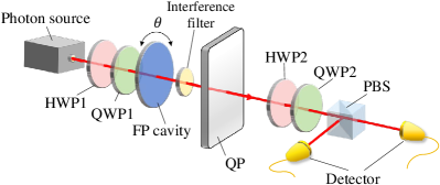
Figure 1: Schematic illustration of the experimental setup used to identify the non-Markovianity of single-photon dynamics in birefringent crystal (QP).

When considering the dynamical changes of the polarization states over time, let us assume that the principal system and its environment are initially prepared in the states $\rho^{S}_{0}=\ket{\lambda}\!\!\bra{\lambda}$ and $\rho^{E}_{0}=\ket{\Omega^{\theta}}\!\!\bra{\Omega^{\theta}}$, respectively. Hence, after their interaction described by $U(t)$, the final state $\rho^{S}_{t}$ of the system can be obtained by performing a partial trace over the environment $\rho^{E}_{t}$. That is,

$$\rho_{S}(t)\!=\!\text{tr}_{E}\!\left[U(t)\left(\rho_{S}(0)\!\otimes\!\rho_{E}(0)\right)U^{\dagger}(t)\right].$$ (8)

In order to completely and quantitatively describe the dynamics of the principal system, let the quantum operations formalism [3, 38, 39] be used to construct a dynamical map relating $\rho_{S}(0)$ to $\rho_{S}(t)$ as $\chi_{t}:\rho_{S}(0)\mapsto\rho_{S}(t)$. The final state can then be represented explicitly as

$$\rho_{S}(t)=\chi^{\theta}_{t}(\rho_{S}(0))=\sum_{m=1}^{4}\sum_{n=1}^{4}\chi^{\theta}_{t,mn}M_{m}\rho_{S}(0)M_{n}^{\dagger},$$ (9)

where $M_{1}=I$, $M_{2}=X$, $M_{3}=-iY$, $M_{4}=Z$, and $I$ and $X$, $Y$, $Z$ denote the identity operator and the Pauli matrices, respectively. The coefficients $\chi^{\theta}_{t,mn}$ are obtained by comparing Eqs. (8) and (9) and constitute a so-called process matrix for the dynamical map of the polarization state, i.e.,

$$\chi^{\theta}_{t}=\frac{1}{4}\left[\begin{matrix}2+\kappa^{\theta}(t)+\kappa^{\theta*}(t)&0&0&\kappa^{\theta}(t)-\kappa^{\theta*}(t)\\ 0&0&0&0\\ 0&0&0&0\\ \kappa^{\theta*}(t)-\kappa^{\theta}(t)&0&0&2-\kappa^{\theta}(t)-\kappa^{\theta*}(t)\\ \end{matrix}\right].$$ (10)

The decoherence factor $\kappa^{\theta}(t)$ in Eq. (10) is given by the corresponding frequency distribution at a specific angle $\theta$ of the FP cavity, i.e.,

$$\kappa^{\theta}(t)=\int d\omega\left|f^{\theta}(\omega)\right|^{2}e^{i\omega\Delta nt},$$ (11)

where $\Delta n={n}_{V}-{n}_{H}$ depends on the particular specification of the quartz plate.

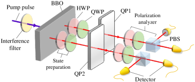
Figure 2: Schematic illustration of the experimental setup used to identify the non-Markovianity of two-photon dynamics in birefringent crystals (QP1,QP2).

III.1.2 Two-photon experiment

The identification of non-Markovian dynamics in two-photon scenarios was investigated using the experimental system implemented in Ref. [31], consisting of entangled photon pairs generated through a spontaneous parametric down-conversion (SPDC) process in a $\beta$-barium borate (BBO) crystal with an ultraviolet pump pulse (Fig. 2). In conducting the investigation, an interference filter was used to control the spectral width $\delta$ of the pump pulse and prepare the frequency state $\ket{\Omega}=\int d\omega_{1}d\omega_{2}g(\omega_{1},\omega_{2})\ket{\omega_{1}}\!\otimes\!\ket{\omega_{2}}$. Note that $g(\omega_{1},\omega_{2})$ denotes the probability amplitude of finding a state $\ket{\omega_{1}}\!\otimes\!\ket{\omega_{2}}$ of a photon pair with frequency $\omega_{1}$ in spatial mode 1 and a photon with frequency $\omega_{2}$ in spatial mode 2. The polarization degrees of freedom of the two photons were initially prepared for an arbitrary state: $\ket{\psi}=a\!\ket{0}\!\otimes\!\ket{0}\!+\!b\!\ket{0}\!\otimes\!\ket{1}\!+\!c\!\ket{1}\!\otimes\!\ket{0}\!+\!d\!\ket{1}\!\otimes\!\ket{1}$, where $\ket{0}\equiv\ket{H}$ and $\ket{1}\equiv\ket{V}$ denote the horizontal and vertical states, respectively, using a pair of QWPs and HWPs. The two degrees of freedom of each photon were then locally coupled in two quartz plates (QP1, QP2). In general, the local interaction in each quartz plate at an active time $t$ can be described by the unitary transformation $U_{i}(t)\ket{\lambda}\otimes\ket{\omega_{i}}=e^{i{\omega_{i}}n_{\lambda}t}\ket{\lambda}\otimes\ket{\omega_{i}}$, where $\lambda=H,V$ and $i$=1, 2 represents the two subsystems. Note that the active times of the single-photon interactions in QP1 and QP2, respectively, are non-overlapping and consecutive. In particular, QP1 activates before QP2. Finally, the tomography of the polarization states was measured by a pair of polarization analyzers.

Let us assume that the principal system and its environment are initially prepared in the states $\rho_{S}(0)=\ket{\psi}\!\!\bra{\psi}$ and $\rho_{E}(0)=\ket{\Omega}\!\!\bra{\Omega}$, respectively. The final state $\rho^{S}_{t}$ of the system can be obtained by performing a partial trace over the environment, i.e.,

$$\rho_{S}(t)\!=\!\text{tr}_{E}\!\left\{\left[\bigotimes_{i=1}^{2}\!U_{i}(t)\right]\!\!\rho_{S}(0)\!\otimes\!\rho_{E}(0)\!\!\left[\bigotimes_{i=1}^{2}U^{\dagger}_{i}(t)\right]\!\right\}.$$ (12)

The final state of the principal system when using the dephasing model can then be written as

$$\rho_{S}(t)\!=\!\!\left[\begin{matrix}|a|^{2}&ab^{\ast}\kappa_{2}(t)&ac^{\ast}\kappa_{1}(t)&ad^{\ast}\kappa_{12}(t)\\ ba^{\ast}\kappa^{\ast}_{2}(t)&|b|^{2}&bc^{\ast}\Lambda_{12}(t)&bd^{\ast}\kappa_{1}(t)\\ ca^{\ast}\kappa^{\ast}_{1}(t)&cb^{\ast}\Lambda^{\ast}_{12}(t)&c^{2}&cd^{\ast}\kappa_{2}(t)\\ da^{\ast}\kappa^{\ast}_{12}(t)&db^{\ast}\kappa^{\ast}_{1}(t)&dc^{\ast}\kappa^{\ast}_{2}(t)&|d|^{2}\\ \end{matrix}\right]\!,$$ (13)

where $\kappa_{1}(t)$, $\kappa_{2}(t)$, $\kappa_{12}(t)$ and $\Lambda_{12}(t)$ denote the decoherence functions of the dephasing model [32]. In terms of the Fourier transform of the joint frequency distribution, $P(\omega_{1},\omega_{2})\equiv|g(\omega_{1},\omega_{2})|^{2}$ [32]:

$$G(\tau_{1},\tau_{2})= \int d\omega_{1}d\omega_{2}P(\omega_{1},\omega_{2})e^{-i\Delta n(\omega_{1}\tau_{1}+\omega_{2}\tau_{2})}$$

$$= e^{\frac{1}{2}[i\omega_{0}\Delta n(\tau_{1}+\tau_{2})-C\Delta n^{2}(\tau_{1}^{2}+\tau_{2}^{2}+2K\tau_{1}\tau_{2})]},$$ (14)

the decoherence functions in $\rho_{S}(t)$ can be expressed as $\kappa_{1}(t)=G(\tau_{1},0)$, $\kappa_{2}(t)=G(0,\tau_{2})$, $\kappa_{12}(t)=G(\tau_{1},\tau_{2})$, $\Lambda_{12}(t)=G(\tau_{1},-\tau_{2})$, where $\omega_{0}$ is the center frequency of the pump pulse; $\tau_{1}$ and $\tau_{2}$ are the active times of the quartz plate in spatial mode 1 and spatial mode 2, respectively; and $C$ is the frequency variance of the single photon generated by the SPDC process.

According to the quantum operation formalism [3, 38, 39], the final state of the system can be represented explicitly as

$$\rho_{S}(t)=\chi^{\delta}_{t}(\rho_{S}(0))=\sum_{m=1}^{16}\sum_{n=1}^{16}\chi^{\delta}_{t,mn}E_{m}\rho_{S}(0)E_{n}^{\dagger},$$ (15)

where $E_{m(n)}=\ket{h}\!\!\bra{r}\otimes\ket{l}\!\!\bra{s}$, in which $m(n)=s\cdot 2^{0}+r\cdot 2^{1}+l\cdot 2^{2}+h\cdot 2^{3}+1$. The coefficients, $\chi_{t,mn}$, can be obtained by comparing Eqs. (13) and (15) and then used to construct a process matrix which describes the dynamical mapping of the two qubits (refer to Ref. [38]), i.e.,

$$\chi^{\delta}_{t}=\frac{1}{4}\left[\begin{matrix}A&Z_{1}&B\\ Z^{\dagger}_{1}&Z_{2}&Z^{\dagger}_{1}\\ B^{\dagger}&Z_{1}&A\\ \end{matrix}\right],$$ (16)

where $A$ and $B$ are $6\times 6$ matrices with the forms

$$A_{kj}\!\!=\!\!\left\{\!\!\begin{array}[]{rcl}1&&\!\!k=j=1,6\\ \kappa_{2}(t)&&\!\!k=1,j=6\\ \kappa^{\ast}_{2}(t)&&\!\!k=6,j=1\\ 0&&\!\!\rm{otherwise}\end{array}\right.,B_{kj}\!\!=\!\!\left\{\!\!\begin{array}[]{rcl}\kappa_{1}(t)&&\!\!k=j=1,6\\ \kappa_{12}(t)&&\!\!k=1,j=6\\ \Lambda_{12}(t)&&\!\!k=6,j=1\\ 0&&\!\!\rm{otherwise}\end{array}\right.,$$ (17)

in which $Z_{1}$ is a $6\times 4$ zero matrix, and $Z_{2}$ is a $4\times 4$ zero matrix. $\chi_{t}$ is completely positive and trace-preserving by definition, as illustrated in Eq. (16).

The local dynamics of the subsystems can also be described by a process matrix, denoted as $\chi^{\prime}_{t}$, which maps the input space of the different subsystems to the same output space, i.e.,

$$\rho_{Si}(t)=\chi^{\prime}_{t}(\rho_{Si}(0))=\sum_{m=1}^{4}\sum_{n=1}^{4}\chi^{\prime}_{t,mn}M_{m}\rho_{Si}(0)M_{n}^{\dagger},$$ (18)

where $M_{m(n)}=\ket{l}\!\!\bra{s}$, in which $m(n)=s\cdot 2^{0}+l\cdot 2^{1}+1$, and $\chi^{\prime}_{t,mn}$ has the following concrete matrix form:

$$\chi^{\prime}_{t}=\frac{1}{2}\left[\begin{matrix}1&0&0&\kappa_{1}(t)\\ 0&0&0&0\\ 0&0&0&0\\ \kappa^{\ast}_{1}(t)&0&0&1\\ \end{matrix}\right].$$ (19)

III.2 Identification results for photonic experiments in previous studies

In the experimental works of Refs. [30, 31], the non-Markovianity of the photon dynamics was identified using the BLP criterion based on the dynamical change of the trace distance between two system states.

III.2.1 Single-photon case

In Ref. [30] for single-photon dynamics, the optimized two initial system states of the single photon were prepared as $\rho^{S}_{0,1}=\outerproduct{+}{+}$ and $\rho^{S}_{0,2}=\outerproduct{-}{-}$, respectively, where $\ket{\pm}=(\ket{H}\pm\ket{V})/\sqrt{2}$. The identification results showed that for environmental conditions (FP cavity angles) of $\theta=6.0^{\circ}$ and $7.5^{\circ}$, the photon dynamics could not be determined as non-Markovian dynamics. However, for angles of $\theta\leq 4.0^{\circ}$ and $\theta\geq 8.0^{\circ}$, the BLP criterion identified non-Markovian photon dynamics.

III.2.2 Two-photon case

For the two-photon dynamics case considered in Ref. [31], the optimized two initial system states were prepared as $\rho^{S}_{0,1}=\outerproduct{\phi^{+}}{\phi^{+}}$ and $\rho^{S}_{0,2}=\outerproduct{\phi^{-}}{\phi^{-}}$, respectively, where $\ket{\phi^{\pm}}=(\ket{HH}\pm\ket{VV})/\sqrt{2}$. The resulting amounts of non-Markovianity were found to be: $(\rm I)~{}\mathcal{N}_{\rm BLP}=0.48$, $(\rm II)~{}\mathcal{N}_{\rm BLP}=0.23$, $(\rm III)~{}\mathcal{N}_{\rm BLP}=0.14$, $(\rm IV)~{}\mathcal{N}_{\rm BLP}=0.02$, corresponding to four different pulse spectra [full width at half maximum (FWHM), denoted as $\delta$] and frequency correlations ($K$), i.e.,

$$\rm(I)\ \delta=0.18~{}nm:{\it K}=-0.92,$$

$$\rm(II)\ \delta=0.52~{}nm:{\it K}=-0.66,$$

$$\rm(III)\ \delta=0.73~{}nm:{\it K}=-0.55,$$ (20)

$$\rm(IV)\ \delta=1.89~{}nm:{\it K}=-0.17.$$

According to the BLP criterion, the dynamics of the entangled photon pairs was identified as non-Markovian under all four conditions (I)-(IV). However, the dynamics of the individual photons in the two-photon system could not be classified as non-Markovian. Moreover, the non-Markovianity of the principal system dynamics increased as $|K|$ increased. Thus, it was inferred that the initial correlations between the local parts of different environments can lead to nonlocal memory effects in the global dynamics. (It is noted that this inference is consistent with the theoretical prediction in Ref. [32].)

IV Identification and quantification of non-Markovian dynamics

IV.1 Determining non-Markovian dynamics by eigenvalues of $\Lambda_{t_{2},t_{1}}$

Based on the dynamics described by the time-local master equation [Eq. (3)], one of the most important characteristics of Markovian dynamics is that it can be arbitrarily divided into two or more legitimate CP subprocesses, which satisfies CP-divisibility (4). As represented this condition in process matrices, that is,

$$\chi_{t_{2}}=\Lambda_{t_{2},t_{1}}\circ\chi_{t_{1}},$$ (21)

where the original process $\chi_{t_{2}}$ from time point 0 to $t_{2}$ is divided into a subprocess $\chi_{t_{1}}$ from time point 0 to $t_{1}$ for arbitrary time $t_{1}$ and an intermediate process from time point $t_{1}$ to $t_{2}$ described by the process matrix, denoted as $\Lambda_{t_{2},t_{1}}$. Note that the time order of $t_{2}$ and $t_{1}$ is strictly as follows: $t_{2}\geq t_{1}\geq 0$ (Fig. 3). When the dynamical process is Markovian, the original process $\chi_{t_{2}}$ satisfies CP-divisibility, and $\chi_{t_{1}}$ and $\Lambda_{t_{2},t_{1}}$ are also CP processes $\chi_{\text{CP}}$. However, if $\Lambda_{t_{2},t_{1}}$ is a non-CP process, the original process $\chi_{t_{2}}$ is not CP-divisible, and the dynamics is said to be non-Markovian.

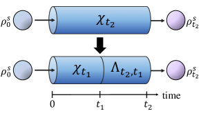
Figure 3: Illustration of the CP-divisibility concept in Markovian dynamics.

In the following, we provide a preliminary experimentally feasible method for identifying non-Markovian dynamics. In particular, we use QPT to characterize $\chi_{t_{2}}$ and $\chi_{t_{1}}$ and calculate the intermediate process $\Lambda_{t_{2},t_{1}}$ by $\chi_{t_{2}}$ and the inverse matrix of $\chi_{t_{1}}$ as follows:

$$\Lambda_{t_{2},t_{1}}=\chi_{t_{2}}\chi_{t_{1}}^{-1}.$$ (22)

If the dynamical process under consideration is Markovian, the original process $\chi_{t_{2}}$ has CP-divisibility. In addition, $\Lambda_{t_{2},t_{1}}$ is also a CP process and all of its eigenvalues are non-negative [12]. However, if even one of the eigenvalues is negative, then $\Lambda_{t_{2},t_{1}}$ is a non-CP process, and hence $\chi_{t_{2}}$ is non-Markovian dynamics. It is noted that this identification method is qualitative rather than quantitative in nature. Thus, having performed preliminary identification, the degree of non-Markovianity is further quantified using the non-Markovian process robustness measure introduced in Sec. IV.2.

IV.2 Non-Markovian process robustness

The non-Markovian process robustness based on CP-divisibility quantifies the degree of non-Markovianity of a dynamical process. In theory, a non-CP intermediate process $\Lambda_{t_{2},t_{1}}$ can become a CP process by mixing with a CP process $\chi^{\prime}$, i.e.,

$$\frac{\Lambda_{t_{2},t_{1}}+b\chi^{\prime}}{1+b}=\chi_{\text{CP}},$$ (23)

where $b\geq 0$. Thus, the non-Markovian process robustness $\beta$ of the intermediate process $\Lambda_{t_{2},t_{1}}$ can be quantitatively characterized by the minimum amount of $\chi^{\prime}$ which must be added to it such that it becomes CP process $\chi_{\text{CP}}$ (Fig. 4). That is,

$$\beta\equiv\!\min_{\chi^{\prime}}b\ .$$ (24)

In other words, Eq. (23) can be reformulated as

$$\frac{\Lambda_{t_{2},t_{1}}+\beta\chi^{\prime}}{1+\beta}=\chi_{\text{CP}}.$$ (25)

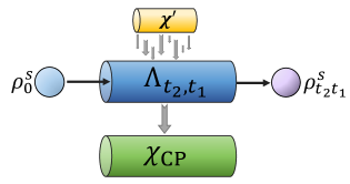
Figure 4: Illustration of non-Markovian process robustness $\beta$.

The minimum amount of $\chi^{\prime}$ can be determined by solving the following optimization equation via semidefinite programming (SDP) with MATLAB [40, 41]:

$$\beta\!=\!\min_{\chi_{\text{CP}}}[\,\text{tr}(\,\chi_{\text{CP}})\,-1]\,,$$ (26)

where the solution constraints are specified as

$$\chi_{\text{CP}}\geq 0,$$ (27)

$$\chi_{\text{CP}}-\chi_{t_{2}}\chi_{t_{1}}^{-1}\geq 0,$$ (28)

$$\text{tr}(\,\chi_{\text{CP}})\,\geq 1.$$ (29)

The first constraint guarantees that $\chi_{\text{CP}}$ is CP, while the second constraint ensures that $\chi^{\prime}$ is also CP. Finally, the third constraint guarantees that $\beta\geq 0$. For instance, when $\Lambda_{t_{2},t_{1}}$ is a non-CP process, the amount of operations $\chi^{\prime}$ required to be added to make it CP is quantified by $\beta$, where $\beta$ is greater than zero. The minimum value of $\beta$ represents the minimum amount of additional operations required and is equal to the sum of the absolute values of all the negative eigenvalues of $\Lambda_{t_{2},t_{1}}$. Conversely, if $\Lambda_{t_{2},t_{1}}$ is already a CP process, no additional operations $\chi^{\prime}$are required, and $\beta$ is equal to zero.

In the following, we demonstrate that non-Markovianity can be regarded as a type of quantum process capability (QPC) [36] through the non-Markovian process robustness $\beta$ [Eq. (25)]. In other words, a non-Markovian process can be regarded as a capable process for manifesting itself in non-Markovianity (denoted as $\chi_{\mathcal{C}}$). Conversely, a process without non-Markovianity can be regarded as an incapable process for non-Markovianity (denoted as $\chi_{\mathcal{I}}$). As described above, the non-Markovian process robustness $\beta$ [Eq. (25)] identifies the non-Markovianity of a process from the perspective of the dynamical process. $\beta$ is thus a sensible measure of QPC for non-Markovianity and should satisfy the conditions for a sensible measure accordingly [36]. In particular, for a sensible measure $C(\Lambda_{t_{2},t_{1}})$ to faithfully quantify non-Markovianity, it should satisfy the following three conditions:

(MP1) Faithfulness: $C(\Lambda_{t_{2},t_{1}})=0$ if and only if $\Lambda_{t_{2},t_{1}}$ is incapable.

(MP2) Monotonicity: $C(\Lambda_{t_{2},t_{1}}\circ\chi_{\text{CP}})\leq C(\Lambda_{t_{2},t_{1}})$, the degree of non-Markovianity of $\Lambda_{t_{2},t_{1}}$ does not increase when applying additional incapable processes, i.e., CP processes.

(MP3) Convexity: $C(\sum_{n}p_{n}\Lambda_{t_{2},t_{1}}\circ\chi_{\text{CP}n})\leq\sum_{n}p_{n}C(\Lambda_{t_{2},t_{1}}\circ\chi_{\text{CP}n})$, the mixing of processes does not increase the non-Markovianity.

The proofs of these three conditions are provided as follows:
$Proof\ of$ (MP1)
The non-Markovian process robustness $\beta$ satisfies (MP1) directly according to the definition of $\beta$. That is, when $\Lambda_{t_{2},t_{1}}$ is a CP-process, (i.e., an incapable process), the value of $\beta$ is zero.
$Proof\ of$ (MP2)
The process of $\Lambda_{t_{2},t_{1}}$ incorporated with incapable processes $\chi_{\mathcal{I}n}$ can be represented in the form shown in equation (25) as follows:

$$\begin{aligned} \Lambda_{t_{2},t_{1}}\circ\chi_{\text{CP}}&=[(1+\beta)\chi_{\text{CP}}-\beta\chi^{\prime}]\circ\chi_{\text{CP}}\\ &=(1+\beta)\chi_{\text{CP}}\circ\chi_{\text{CP}}-\beta\chi^{\prime}\circ\chi_{\text{CP}}\\ &=(1+\beta^{\prime})\chi_{\text{CP}}-\beta^{\prime}\chi^{\prime}.\end{aligned}$$ (30)

Since $\chi_{\text{CP}}$ is an incapable process, $\chi_{\text{CP}}\circ\chi_{\text{CP}}$ must also be an incapable process. Thus, the optimal $\beta^{\prime}$ value of $\Lambda_{t_{2},t_{1}}\circ\chi_{\text{CP}}$ must be equal to or less than the optimal $\beta$ value of $\Lambda_{t_{2},t_{1}}$, i.e., $\beta^{\prime}\leq\beta$.
$Proof\ of$ (MP3)
Let $\sum_{n}p_{n}\Lambda_{t_{2},t_{1}}\circ\chi_{\text{CP}n}$ be represented as

$$\begin{aligned} \sum_{n}p_{n}\Lambda_{t_{2},t_{1}}\circ\chi_{\text{CP}n}=(1+b^{\prime})\chi_{\text{CP}^{\prime}}-b^{\prime}\chi^{\prime\prime},\end{aligned}$$ (31)

where

$$\begin{aligned} \chi_{\text{CP}^{\prime}}&=\frac{\sum_{n}p_{n}(1+\beta_{n})\chi_{\text{CP}n}}{1+b^{\prime}},\\ \chi^{\prime\prime}&=\frac{\sum_{n}p_{n}\beta_{n}\chi^{\prime}_{n}}{b^{\prime}},\\ b^{\prime}&=\sum_{n}p_{n}\beta_{n}=\sum_{n}p_{n}C(\Lambda_{t_{2},t_{1}}\circ\chi_{\text{CP}n}),\end{aligned}$$ (32)

and $\chi^{\prime}_{n}$ is the CP process for each $\Lambda_{t_{2},t_{1}}\circ\chi_{\text{CP}n}$. Since $\beta=C(\sum_{n}p_{n}\Lambda_{t_{2},t_{1}}\circ\chi_{\text{CP}n})$ is the optimal $b$ in Eq. (23), then $\beta\leq b^{\prime}$.

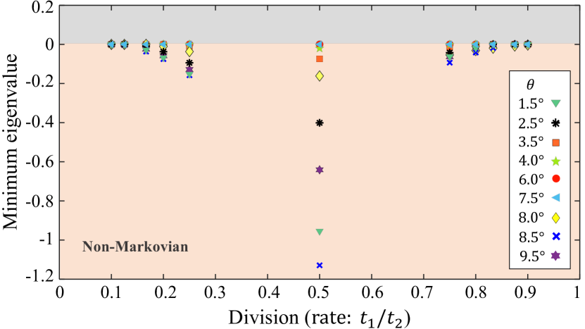
Figure 5: Single-photon dynamics in different divisions. We chose eleven divisions for the original process in single-photon dynamics according to Eq. (21). We then observed whether there existed a negative value among the minimum eigenvalue of the intermediate process of the photon dynamics under various environmental conditions in the different divisions to make a preliminary identification of the dynamics as non-Markovian.

IV.3 Identification of non-Markovianity of photon dynamics in birefringent crystals by non-Markovian process robustness

The validity of the experimentally feasible method proposed in Sec. IV.2 for the identification of non-Markovianity based on the concept of CP-divisibility, i.e., the non-Markovian process robustness $\beta$ [Eq. (25)], was evaluated by investigating the non-Markovianity of the single-photon [30] and two-photon [31] dynamics described in Sec. III. Reference [37] and Appendix A systematically determined the information of the decoherence functions in Eqs. (11, III.1.2) and constructed the process matrix $\chi_{t_{2}}=\chi^{\theta}_{t_{2}}$ [Eq. (10)] and $\chi_{t_{2}}=\chi^{\delta}_{t_{2}}$ [Eq. (16)] for the single-photon and two-photon dynamics cases, respectively, by fitting the experimental data reported in Refs. [30] and [31]. It was found that the simulated trace distance results obtained from the constructed process matrices were highly consistent with the experimental results in Refs. [30] and [31]. Hence, the process matrices are considered to be sufficiently reliable to demonstrate our identification of non-Markovianity in the single-photon [30] and two-photon [31] systems.

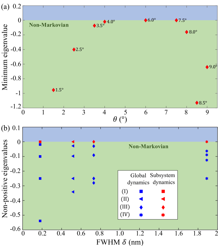
Figure 6: Identification results for determining non-Markovian dynamics in (a) single-photon and (b) two-photon dynamics. We chose to divide the original process $\chi_{t_{2}}$ in half at time $t_{1}$, i.e., $t_{1}=t_{2}/2$. (a) Environmental conditions created by nine different angles of the cavity in the single-photon system, minimum eigenvalues of intermediate processes. (b) Four frequency correlation conditions (III.2.2) in the two-photon system, non-positive eigenvalues of the global system (blue) and subsystem (red).

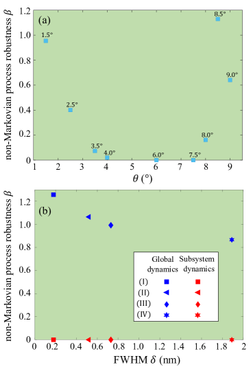
Figure 7: Identification results obtained using the non-Markovian process robustness $\beta$ in (a) single-photon and (b) two-photon dynamics. We chose to divide the original process $\chi_{t_{2}}$ in half at time $t_{1}$, i.e., $t_{1}=t_{2}/2$. (a) $\beta$ for the environmental conditions created by nine different angles of the cavity in the single-photon system. (b) $\beta$ for global dynamics (blue) and subsystem dynamics (red) for four frequency correlation conditions (III.2.2) in the two-photon system.

Accordingly, in the present study, we chose to divide the original process $\chi_{t_{2}}$ in half at time $t_{1}$ according to Eq. (21), i.e., $t_{1}=t_{2}/2$. Since we observed qualitatively through Eq. (22), under different divides, the case of dividing the original process in half can identify more single-photon dynamics with different environmental conditions are non-Markovian, as shown in Fig. 5. An analysis of $\Lambda_{t_{2},t_{1}}$ was then conducted using the non-Markovian process robustness $\beta$ [Eq. (25)] in order to quantitatively characterize the degree of non-Markovianity of $\chi_{t_{2}}$, that is, the QPC of $\chi_{t_{2}}$ for non-Markovianity. The identification results for the single-photon and two-photon dynamics cases are presented in the following:

IV.3.1 Single-photon dynamics

As shown in Fig. 6(a), among the nine different environmental conditions created by rotating the FP cavity, we identified non-Markovian dynamics at cavity angles of $\theta\leq 4.0^{\circ}$ and $\theta\geq 8.0^{\circ}$ through the presence of negative eigenvalues. For $\theta=6.0^{\circ}$ and $7.5^{\circ}$, the minimum eigenvalues of $\Lambda_{t_{2},t_{1}}=\Lambda^{\theta}_{t_{2},t_{1}}$ were equal to zero, and hence it was not possible to confirm the dynamics as either non-Markovian or Markovian dynamics. Thus, given these preliminary identification results, we further quantified the non-Markovianity under the nine environmental conditions using $\beta$ [Eq. (25)], as shown in Fig. 7(a). For angles of $\theta\leq 4.0^{\circ}$ and $\theta\geq 8.0^{\circ}$, $\beta$ had a value greater than zero, which confirms the amount of additional operations $\chi^{\prime}$ in (25) required and is equal to the sum of the absolute values of all negative eigenvalues of $\Lambda^{\theta}_{t_{2},t_{1}}$. By contrast, for $\theta=6.0^{\circ}$ and $7.5^{\circ}$, the photon dynamics has no characteristic of the non-Markovianity, thus no additional operations $\chi^{\prime}$ are required and $\beta$=0.

IV.3.2 Two-photon dynamics

Figure 6(b) shows the preliminary identification results for the global photon dynamics and subsystem photon dynamics for the four frequency correlation conditions (III.2.2) considered in the two-photon experiment in Ref. [31]. It is seen that $\Lambda_{t_{2},t_{1}}=\Lambda^{\delta}_{t_{2},t_{1}}$ has eigenvalues of less than zero for all four global photon dynamics, while the eigenvalues of the intermediate processes are not less than zero for all of the subsystem photon dynamics. Thus, the preliminary identification results indicate that the global photon dynamics is non-Markovian, while the subsystem photon dynamics cannot be confirmed as non-Markovian. However, the $\beta$ robustness results in Fig. 7(b) confirm and quantify the degree of non-Markovianity of the global photon dynamics, while the subsystem photon dynamics has no characteristic of non-Markovianity, $\beta$=0.

IV.3.3 Comparison

The identification results presented in IV.3.1 and IV.3.2 above are consistent with the results presented in Refs. [30] and [31], respectively, using the BLP criterion. For the two-photon dynamics case, the identification results obtained using the non-Markovian process robustness $\beta$ [Eq. (25)] reveal the existence of a nonlocal memory effect. In particular, the global dynamics is non-Markovian, while the local dynamics of both subsystems is Markovian. Notably, suppose there is no optimization of the initial system state pairs. In that case, the BLP criterion only considers certain states and performs trials for witnessing the revival of the trace distance between the two system states. By contrast, we identify non-Markovian dynamics from the perspective of the dynamical process by performing QPT to fully characterize the information of the process without optimizing the initial states. Thus, the proposed method will not fail to identify non-Markovian dynamics simply as a result of inappropriate state selection.

V Efficient identification of non-Markovian dynamics

This section commences by examining the number of experimental settings required when using the non-Markovian process robustness $\beta$ [Eq. (25)] to quantify the degree of non-Markovianity. A more efficient method based on CP-divisibility is then proposed for identifying non-Markovian dynamics. Finally, the proposed method is employed to identify the non-Markovian dynamics of the single-photon and two-photon systems in Refs. [30] and [31], respectively.

V.1 Number of experimental settings required for $\beta$ [Eq. (25)]

QPT provides the means to obtain all the information about a process. However, the complete QPT procedure requires the input of several states and the subsequent performance of quantum state tomography (QST). For example, the non-Markovian process robustness $\beta$ [Eq. (25)] requires QPT for $\chi_{t_{2}}$ and $\chi_{t_{1}}$ to quantify the value of $\beta$ for the intermediate process $\Lambda_{t_{2},t_{1}}$ though Eq. (22). In single-photon dynamics, a process requires a minimum of four input states to perform QPT to characterize and then construct the process. Furthermore, these four states all require the performance of QST to reconstruct the state by performing experimental measurements of the observables $X$, $Y$, and $Z$. Thus, a total of twelve experimental settings are required to be performed to complete the QPT procedure. Similarly, performing QPT for two-photon dynamics requires at least sixteen input states to construct the process. These sixteen states each require the performance of QST to reconstruct the state by performing experimental measurements of the observables, which are products of the Pauli matrices, i.e., $XX$, $XY$, $XZ$, $YX$, $YY$, $YZ$, $ZX$, $ZY$, and $ZZ$. In other words, a total of 144 experimental settings are required to complete the QPT procedure. As described above, when implementing the non-Markovian process robustness $\beta$ [Eq. (25)] , it is necessary to perform QPT for $\chi_{t_{2}}$ and $\chi_{t_{1}}$. Therefore, a total of 24 and 288 experimental settings are required to characterize single-photon and two-photon dynamics, respectively.

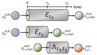
Figure 8: Illustration of the proposed method for the efficient identification of non-Markovian dynamics.

Table 1: Efficient identification results for single-photon non-Markovian dynamics with two initial states $\rho^{A}_{0}$, $\rho^{B}_{0}$.

Seleted states	Conditions ($\theta$)
$\rho^{A}_{0}$, $\rho^{B}_{0}$	$1.5^{\circ}$	$2.5^{\circ}$	$3.5^{\circ}$	$4.0^{\circ}$	$6.0^{\circ}$	$7.5^{\circ}$	$8.0^{\circ}$	$8.5^{\circ}$	$9.0^{\circ}$
$\outerproduct{H}{H}$, $\outerproduct{V}{V}$	2	2	2	2	2	2	2	2	2
$\outerproduct{H}{H}$, $\outerproduct{+}{+}$	2.2325	2.1752	2.0577	2.0179	2	2	2.1078	2.2464	2.2125
$\outerproduct{H}{H}$, $\outerproduct{-}{-}$	2.2325	2.1752	2.0577	2.0179	2	2	2.1078	2.2464	2.2125
$\outerproduct{H}{H}$, $\outerproduct{R}{R}$	2.2325	2.1752	2.0577	2.0179	2	2	2.1078	2.2464	2.2125
$\outerproduct{H}{H}$, $\outerproduct{L}{L}$	2.2325	2.1752	2.0577	2.0179	2	2	2.1078	2.2464	2.2125
$\outerproduct{V}{V}$, $\outerproduct{+}{+}$	2.2325	2.1752	2.0577	2.0179	2	2	2.1078	2.2464	2.2125
$\outerproduct{V}{V}$, $\outerproduct{-}{-}$	2.2325	2.1752	2.0577	2.0179	2	2	2.1078	2.2464	2.2125
$\outerproduct{V}{V}$, $\outerproduct{R}{R}$	2.2325	2.1752	2.0577	2.0179	2	2	2.1078	2.2464	2.2125
$\outerproduct{V}{V}$, $\outerproduct{L}{L}$	2.2325	2.1752	2.0577	2.0179	2	2	2.1078	2.2464	2.2125
$\outerproduct{+}{+}$, $\outerproduct{-}{-}$	2.9080	2.5342	2.1312	2.0381	2	2	2.2659	2.9989	2.7328
$\outerproduct{+}{+}$, $\outerproduct{R}{R}$	2.733	2.4651	2.1270	2.0377	2	2	2.2496	2.7974	2.6134
$\outerproduct{+}{+}$, $\outerproduct{L}{L}$	2.733	2.4651	2.1270	2.0377	2	2	2.2496	2.7974	2.6134
$\outerproduct{-}{-}$, $\outerproduct{R}{R}$	2.733	2.4651	2.1270	2.0377	2	2	2.2496	2.7974	2.6134
$\outerproduct{-}{-}$, $\outerproduct{L}{L}$	2.733	2.4651	2.1270	2.0377	2	2	2.2496	2.7974	2.6134
$\outerproduct{R}{R}$, $\outerproduct{L}{L}$	2.9080	2.5342	2.1312	2.0381	2	2	2.2659	2.9989	2.7328

Table 2: Efficient identification results for non-Markovianity of two-photon global dynamics with two initial states $\rho^{A}_{0}$, $\rho^{B}_{0}$.

Seleted states	Conditions (III.2.2)
$\rho^{A}_{0}$, $\rho^{B}_{0}$	(I)	(II)	(III)	(IV)
$\outerproduct{\phi^{+}}{\phi^{+}}$, $\outerproduct{\phi^{-}}{\phi^{-}}$	3.7245	3.0667	2.8188	2.3567
$\outerproduct{\phi^{+}}{\phi^{+}}$, $\outerproduct{\psi^{+}}{\psi^{+}}$	3.7245	3.0667	2.8188	2.3567
$\outerproduct{\phi^{+}}{\phi^{+}}$, $\outerproduct{\psi^{-}}{\psi^{-}}$	3.7245	3.0667	2.8188	2.3567
$\outerproduct{\phi^{-}}{\phi^{-}}$, $\outerproduct{\psi^{+}}{\psi^{+}}$	3.7245	3.0667	2.8188	2.3567
$\outerproduct{\phi^{-}}{\phi^{-}}$, $\outerproduct{\psi^{-}}{\psi^{-}}$	3.7245	3.0667	2.8188	2.3567
$\outerproduct{\psi^{+}}{\psi^{+}}$, $\outerproduct{\psi^{-}}{\psi^{-}}$	2.0594	2.0874	2.0871	2.1801
$\outerproduct{S_{1}}{S_{1}}$, $\outerproduct{S_{2}}{S_{2}}$	2.7437	2.4938	2.3925	2.2629
$\outerproduct{S_{1}}{S_{1}}$, $\outerproduct{S_{3}}{S_{3}}$	3.1098	2.7337	2.5815	2.3122
$\outerproduct{S_{1}}{S_{1}}$, $\outerproduct{S_{4}}{S_{4}}$	3.1098	2.7337	2.5815	2.3122
$\outerproduct{S_{2}}{S_{2}}$, $\outerproduct{S_{3}}{S_{3}}$	3.1098	2.7337	2.5815	2.3122
$\outerproduct{S_{2}}{S_{2}}$, $\outerproduct{S_{4}}{S_{4}}$	3.1098	2.7337	2.5815	2.3122
$\outerproduct{S_{3}}{S_{3}}$, $\outerproduct{S_{4}}{S_{4}}$	2.7437	2.4938	2.3925	2.2629
$\outerproduct{HH}{HH}$, $\outerproduct{VV}{VV}$	2	2	2	2
$\outerproduct{HH}{HH}$, $\outerproduct{HV}{HV}$	2	2	2	2
$\outerproduct{HH}{HH}$, $\outerproduct{H+}{H+}$	2	2	2	2
$\outerproduct{HH}{HH}$, $\outerproduct{HR}{HR}$	2	2	2	2
$\outerproduct{HH}{HH}$, $\outerproduct{++}{++}$	2.7946	2.4263	2.3038	2.0558
$\outerproduct{HH}{HH}$, $\outerproduct{RR}{RR}$	2.7946	2.4263	2.3038	2.0558
$\outerproduct{++}{++}$, $\outerproduct{--}{--}$	3.5892	2.8525	2.6075	2.1116
$\outerproduct{++}{++}$, $\outerproduct{H+}{H+}$	3.5892	2.8525	2.6075	2.1116
$\outerproduct{++}{++}$, $\outerproduct{HR}{HR}$	2.7946	2.4263	2.3038	2.0558
$\outerproduct{++}{++}$, $\outerproduct{RR}{RR}$	3.5892	2.8525	2.6075	2.1116
$\outerproduct{--}{--}$, $\outerproduct{H-}{H-}$	3.5892	2.8525	2.6075	2.1116
$\outerproduct{RR}{RR}$, $\outerproduct{LL}{LL}$	3.5892	2.8525	2.6075	2.1116

Table 3: Efficient identification results for non-Markovianity of two-photon subsystem dynamics with two initial states $\rho^{A}_{0}$, $\rho^{B}_{0}$.

Seleted states	Conditions (III.2.2)
$\rho^{A}_{0}$, $\rho^{B}_{0}$	(I)	(II)	(III)	(IV)
$\outerproduct{H}{H}$, $\outerproduct{V}{V}$	2	2	2	2
$\outerproduct{H}{H}$, $\outerproduct{+}{+}$	2	2	2	2
$\outerproduct{H}{H}$, $\outerproduct{-}{-}$	2	2	2	2
$\outerproduct{H}{H}$, $\outerproduct{R}{R}$	2	2	2	2
$\outerproduct{H}{H}$, $\outerproduct{L}{L}$	2	2	2	2
$\outerproduct{V}{V}$, $\outerproduct{+}{+}$	2	2	2	2
$\outerproduct{V}{V}$, $\outerproduct{-}{-}$	2	2	2	2
$\outerproduct{V}{V}$, $\outerproduct{R}{R}$	2	2	2	2
$\outerproduct{V}{V}$, $\outerproduct{L}{L}$	2	2	2	2
$\outerproduct{+}{+}$, $\outerproduct{-}{-}$	2	2	2	2
$\outerproduct{+}{+}$, $\outerproduct{R}{R}$	2	2	2	2
$\outerproduct{+}{+}$, $\outerproduct{L}{L}$	2	2	2	2
$\outerproduct{-}{-}$, $\outerproduct{R}{R}$	2	2	2	2
$\outerproduct{-}{-}$, $\outerproduct{L}{L}$	2	2	2	2
$\outerproduct{R}{R}$, $\outerproduct{L}{L}$	2	2	2	2

Table 4: Efficient identification results for single-photon non-Markovian dynamics with one initial state $\rho^{A}_{0}$.

Seleted states	Conditions ($\theta$)
$\rho^{A}_{0}$	$1.5^{\circ}$	$2.5^{\circ}$	$3.5^{\circ}$	$4.0^{\circ}$	$6.0^{\circ}$	$7.5^{\circ}$	$8.0^{\circ}$	$8.5^{\circ}$	$9.0^{\circ}$
$\outerproduct{H}{H}$	1	1	1	1	1	1	1	1	1
$\outerproduct{V}{V}$	1	1	1	1	1	1	1	1	1
$\outerproduct{+}{+}$	1	1	1	1	1	1	1	1	1
$\outerproduct{-}{-}$	1	1	1	1	1	1	1	1	1
$\outerproduct{R}{R}$	1	1	1	1	1	1	1	1	1
$\outerproduct{L}{L}$	1	1	1	1	1	1	1	1	1

Table 5: Efficient identification results for non-Markovianity of two-photon dynamics with one initial state $\rho^{A}_{0}$.

Seleted states	Conditions (III.2.2)
$\rho^{A}_{0}$	(I)	(II)	(III)	(IV)
$\outerproduct{\phi^{+}}{\phi^{+}}$	1	1	1	1
$\outerproduct{\phi^{-}}{\phi^{-}}$	1	1	1	1
$\outerproduct{\psi^{+}}{\psi^{+}}$	1	1	1	1
$\outerproduct{\psi^{-}}{\psi^{-}}$	1	1	1	1

V.2 Efficient method for identification of non-Markovian dynamics

To reduce the number of experimental settings required to identify non-Markovian dynamics, we propose herein a witness method based on the fact that the process of Markovian dynamics satisfies CP-divisibility. As shown in Fig. 8, the proposed method simply prepares a minimum of two initial states $\rho^{A}_{0}$ and $\rho^{B}_{0}$ of the same basis states or different basis states. These states are input to both the completely unknown process $\mathcal{E}_{t_{2}}$ and the divided two subprocesses $\mathcal{E}_{t_{1}}$, $\Lambda_{t_{2},t_{1}}$ of the unknown process. An inspection is then made of whether the final states $\rho^{A}_{t_{2}t_{1}}$ and $\rho^{B}_{t_{2}t_{1}}$ of $\mathcal{E}_{t_{1}}\circ\Lambda_{t_{2},t_{1}}$ are different from the final states $\rho^{A}_{t_{2},\text{expt}}$ and $\rho^{B}_{t_{2},\text{expt}}$ of $\mathcal{E}_{t_{2}}$. Due to CP-divisibility of Markovian dynamics, the intermediate process $\Lambda_{t_{2},t_{1}}$ is also a CP process when the dynamics is Markovian, and the output states $\rho^{A}_{t_{2}t_{1}}$, $\rho^{B}_{t_{2}t_{1}}$ are positive after $\mathcal{E}_{t_{1}}\circ\Lambda_{t_{2},t_{1}}$. Similarly, the output states $\rho^{A}_{t_{2}t_{1}}$, $\rho^{B}_{t_{2}t_{1}}$ will also be the same as the output states $\rho^{A}_{t_{2},\text{expt}}$, $\rho^{B}_{t_{2},\text{expt}}$ after $\mathcal{E}_{t_{2}}$, i.e., $\rho^{A}_{t_{2}t_{1}}=\rho^{A}_{t_{2},\text{expt}}$ and $\rho^{B}_{t_{2}t_{1}}=\rho^{B}_{t_{2},\text{expt}}$. However, if the intermediate process $\Lambda_{t_{2},t_{1}}$ is a non-CP process, that is, the dynamics is non-Markovian, $\rho^{A}_{t_{2}t_{1}}$, $\rho^{B}_{t_{2}t_{1}}$ will be different from $\rho^{A}_{t_{2},\text{expt}}$, $\rho^{B}_{t_{2},\text{expt}}$, i.e., $\rho^{A}_{t_{2}t_{1}}\neq\rho^{A}_{t_{2},\text{expt}}$ and $\rho^{B}_{t_{2}t_{1}}\neq\rho^{B}_{t_{2},\text{expt}}$.

To determine whether an intermediate process $\Lambda_{t_{2},t_{1}}$ is a CP process and $\rho^{A}_{t_{2}t_{1}}=\rho^{A}_{t_{2},\text{expt}}$, $\rho^{B}_{t_{2}t_{1}}=\rho^{B}_{t_{2},\text{expt}}$, we assume that a given process is Markovian and $\Lambda_{t_{2},t_{1}}$ is a CP process, denoted as

$$\Lambda_{t_{2},t_{1}}\geq 0.$$ (33)

We further assume that the two initial states $\rho^{A}_{0}$ and $\rho^{B}_{0}$ pass through $\mathcal{E}_{t_{1}}\circ\Lambda_{t_{2},t_{1}}$ to obtain the final states $\rho^{A}_{t_{2}t_{1}}$ and $\rho^{B}_{t_{2}t_{1}}$, which can be written as $\rho^{A}_{t_{2}t_{1}}=\Lambda_{t_{2},t_{1}}(\,\mathcal{E}_{t_{1}}(\,\rho^{A}_{0}\,)\,)$ and $\rho^{B}_{t_{2}t_{1}}=\Lambda_{t_{2},t_{1}}(\,\mathcal{E}_{t_{1}}(\,\rho^{B}_{0}\,)\,)$, respectively. Finally, we assume that $\rho^{A}_{t_{2}t_{1}}$ and $\rho^{B}_{t_{2}t_{1}}$ are both positive, i.e.,

$$\begin{aligned} \rho^{A}_{t_{2}t_{1}}\geq 0,\\ \rho^{B}_{t_{2}t_{1}}\geq 0.\end{aligned}$$ (34)

Therefore, when restricted to

$$\begin{aligned} \rho^{A}_{t_{2}t_{1}}-\rho^{A}_{t_{2},\text{expt}}\geq 0,\\ \rho^{B}_{t_{2}t_{1}}-\rho^{B}_{t_{2},\text{expt}}\geq 0,\end{aligned}$$ (35)

this ensures $\text{tr}(\rho^{A}_{t_{2}t_{1}})\geq 1$ and $\text{tr}(\rho^{B}_{t_{2}t_{1}})\geq 1$. We propose that if $\Lambda_{t_{2},t_{1}}$ is a CP process such that $\rho^{A}_{t_{2}t_{1}}=\rho^{A}_{t_{2},\text{expt}}$, $\rho^{B}_{t_{2}t_{1}}=\rho^{B}_{t_{2},\text{expt}}$ then $\text{tr}(\rho^{A}_{t_{2}t_{1}})=1$, $\text{tr}(\rho^{A}_{t_{2}t_{1}})=1$. However, if $\Lambda_{t_{2},t_{1}}$ is not a CP process, i.e., $\rho^{A}_{t_{2}t_{1}}\neq\rho^{A}_{t_{2},\text{expt}}$, $\rho^{B}_{t_{2}t_{1}}\neq\rho^{B}_{t_{2},\text{expt}}$, then $\text{tr}(\rho^{A}_{t_{2}t_{1}})>1$ and $\text{tr}(\rho^{B}_{t_{2}t_{1}})>1$, and $\mathcal{E}_{t_{2}}$ is non-Markovian dynamics. In other words, non-Markovianity can be identified simply by determining whether the minimum value of the witness $\mathcal{W}$ exceeds 2 via SDP with MATLAB [40, 41] under the constraints (33-35). That is, the witness $\mathcal{W}$ can be written as

$$\mathcal{W}(\rho^{A}_{0},\rho^{B}_{0})\equiv\min_{\Lambda_{t_{2},t_{1}}}[\,\text{tr}(\Lambda_{t_{2},t_{1}}(\,\mathcal{E}_{t_{1}}(\,\rho^{A}_{0}\,)\,))+\text{tr}(\Lambda_{t_{2},t_{1}}(\,\mathcal{E}_{t_{1}}(\,\rho^{B}_{0}\,)\,))\,]>2.$$ (36)

If the unknown process is Markovian, then $\Lambda_{t_{2},t_{1}}$ is a CP process with $\rho^{A}_{t_{2}t_{1}}=\rho^{A}_{t_{2},\text{expt}}$, $\rho^{B}_{t_{2}t_{1}}=\rho^{B}_{t_{2},\text{expt}}$ and $\text{tr}(\rho^{A}_{t_{2}t_{1}})=1$, $\text{tr}(\rho^{A}_{t_{2}t_{1}})=1$, and $\mathcal{W}=2$. If $\mathcal{W}>2$, this may be caused by $\text{tr}(\rho^{A}_{t_{2}t_{1}})>1$, $\text{tr}(\rho^{B}_{t_{2}t_{1}})>1$, or both. In other words, $\Lambda_{t_{2},t_{1}}$ is not a CP process and $\rho^{A}_{t_{2}t_{1}}\neq\rho^{A}_{t_{2},\text{expt}}$, $\rho^{B}_{t_{2}t_{1}}\neq\rho^{B}_{t_{2},\text{expt}}$. Consequently, the unknown process does not satisfy CP-divisibility, and can thus be identified as non-Markovian.

As described above, when applying the proposed efficient identification method, a minimum of just two initial states $\rho^{A}_{0}$, $\rho^{B}_{0}$, are prepared experimentally and the corresponding final states of $\mathcal{E}_{t_{2}}$ and $\mathcal{E}_{t_{1}}$ are obtained via QST as $\rho^{A}_{t_{2},\text{expt}},\rho^{B}_{t_{2},\text{expt}}$ and $\rho^{A}_{t_{1},\text{expt}},\rho^{B}_{t_{1},\text{expt}}$, respectively. For the case of single-photon dynamics, these four final states each require the realization of QST, and consequently a total of 12 experimentally measurable settings are required. Similarly, for the case of two-photon dynamics, the four final states each require the implementation of QST, and hence a total of 36 experimentally measurable settings are required. Thus, when using the proposed efficient method for identifying non-Markovian dynamics, the total number of experimental settings is reduced by 12 compared to the case when using the non-Markovian process robustness $\beta$ [Eq. (25)] for single-photon dynamics and by 252 for the case of two-photon dynamics. However, it is worth noting here that since we chose two initial states, the identification results may be affected by the chosen initial states. Therefore, it may be necessary to perform more than one trial.

V.3 Efficient identification results for non-Markovian dynamics

The experimental feasibility of the proposed efficient method for identifying non-Markovian dynamics was demonstrated using the one-photon [30] and two-photon dynamics [31] reported in the literature. The corresponding results are presented in the following:

V.3.1 Single-photon dynamics

As shown in Table 1, nine different environmental conditions were created by rotating the FP cavity. Moreover, two different initial states were chosen in each trial. For initial states of $\rho^{A}_{0}$ as $\outerproduct{H}{H}$ and $\rho^{B}_{0}$ as $\outerproduct{V}{V}$, the witness (36) was found to have a value of $\mathcal{W}=2$ for all environmental conditions, indicating that there existed an intermediate CP process $\Lambda_{t_{2}t_{1}}$ that satisfied both $\rho^{A}_{t_{2}t_{1}}=\rho^{A}_{t_{2},\text{expt}}$, $\rho^{B}_{t_{2}t_{1}}=\rho^{B}_{t_{2},\text{expt}}$. Given these initial states, it was thus impossible to confirm whether or not the dynamics is non-Markovian. However, when the selected states were chosen as different base states, such as $\outerproduct{H}{H},\outerproduct{+}{+}$ and $\outerproduct{V}{V},\outerproduct{R}{R}$ and so on, or the same base states with coherence, such as $\outerproduct{+}{+},\outerproduct{-}{-}$ and $\outerproduct{R}{R},\outerproduct{L}{L}$, the witness had a value of $\mathcal{W}=2$ for cavity angles of $\theta=6.0^{\circ}$ and $7.5^{\circ}$, but $\mathcal{W}>2$ for all other angles. Here we define $\ket{R}=(\ket{H}+i\ket{V})/\sqrt{2}$ and $\ket{L}=(\ket{H}-i\ket{V})/\sqrt{2}$. Thus, while the dynamics at $\theta=6.0^{\circ},7.5^{\circ}$ still could not be confirmed as non-Markovian, those at $\theta\leq 4.0^{\circ}$ and $\geq 8.0^{\circ}$ were identified as non-Markovian.

V.3.2 Two-photon dynamics

For the global dynamics, two states were chosen from the entangled states as initial states and two states were chosen from the separable states (see Table 2). Considering $\ket{\phi^{+}}$ and $\ket{\phi^{-}}$ of the selected Bell states as an example, the witness was found to have a value of $\mathcal{W}>2$ for all four conditions. Hence, the four dynamics were all identified as non-Markovian. Other selection combinations of the Bell states: $\ket{\phi^{\pm}}$ and $\ket{\psi^{\pm}}=(\ket{HV}\pm\ket{VH})/\sqrt{2}$, and entangled states, e.g., $\ket{S_{1}}=(\ket{H+}+\ket{V-})/\sqrt{2}$, $\ket{S_{2}}=(\ket{H+}-\ket{V-})/\sqrt{2}$, $\ket{S_{3}}=(\ket{H-}+\ket{V+})/\sqrt{2}$, $\ket{S_{4}}=(\ket{H-}-\ket{V+})/\sqrt{2}$, all yielded the same identification results. When selecting separate states, for example, $\ket{HH}$ and $\ket{VV}$, as the initial states, the four dynamics yielded $\mathcal{W}=2$ and thus could not be confirmed as either non-Markovian or Markovian. However, all four dynamics were identified as non-Markovian when states with coherence, such as $\ket{++}$ and $\ket{--}$ or $\ket{++}$ and $\ket{RR}$, were chosen as the initial states. Regarding the local dynamics of these composite dynamics, and taking the photons in arm $1$ passing through QP1 as an example, the complete process of QP1 was divided into two subprocesses, and the two initial states were chosen as the same basis states or different basis states, that is, $\ket{H},\ket{V}$ and $\ket{H},\ket{+}$, and so on (see Table 3). The witness had a value of $\mathcal{W}=2$ under all four experimental conditions. Hence, the dynamics could not be confirmed as non-Markovian.

V.3.3 Discussion and comparison

A further investigation was performed to evaluate the feasibility of the proposed efficient identification method when preparing only one initial state. For this case, Eq. (36) was reformulated as

$$\mathcal{W}(\rho^{A}_{0})\equiv\min_{\Lambda_{t_{2},t_{1}}}[\,\text{tr}(\Lambda_{t_{2},t_{1}}(\,\mathcal{E}_{t_{1}}(\,\rho^{A}_{0}\,)\,))]>1.$$ (37)

Tables 4 and 5 show the corresponding identification results for the single-photon and two-photon dynamics, respectively. In both cases, the identification results are unable to confirm the existence of non-Markovian dynamics. In other words, the efficient identification of non-Markovian dynamics based on CP-divisibility can be performed only when selecting two initial states with quantum characteristics, i.e., superposition and entanglement. In such cases, the identification results are consistent with those obtained using the non-Markovian process robustness $\beta$ [Eq. (25)]. They are all consistent with the results presented in Refs. [30] and [31].

VI Conclusion and outlook

The time-local master equation applies to a much larger class of quantum evolutions than those described by the GKSL master equation for dynamics with the time-independent generator. In particular, the Markovian dynamics defined in the time-local master equation should satisfy CP-divisibility. Therefore CP-divisibility plays a vital role in investigating non-Markovian dynamics. However, experimentally implementing a measure of non-Markovian dynamics underlying CP-divisibility, such as the RHP criterion, still needs to be completed.

In this study, we have proposed two experimentally feasible methods based on CP-divisibility for identifying and quantifying the non-Markovianity of quantum dynamics. The first method exploits the non-Markovian process robustness $\beta$ (Sec. IV), while the second method requires a minimum of just two initial states to efficiently identify non-Markovian dynamics (Sec. V). Moreover, we have shown that non-Markovianity can be regarded as a type of quantum process capability (QPC) through $\beta$ and have additionally proven that $\beta$ satisfies three conditions for a sensible measure of QPC for non-Markovianity. Finally, we have demonstrated the identification of the non-Markovian dynamics of both one-photon and two-photon systems [30, 31] using the two proposed methods.

For the non-Markovian process robustness, our identification of non-Markovian dynamics is from the perspective of the dynamical process by performing quantum process tomography (QPT) to fully characterize the system dynamics without optimizing the initial states, such as the BLP criterion. The implementation of QPT relies on the realization of quantum state tomography (QST), which is required in performing our second method. Therefore our methods proposed in this study can be employed to explore non-Markovianity and the related effects on quantum-information processing in other non-Markovian dynamical systems where QST is implementable, such as the estimation error threshold of non-Markovian effect-tolerant quantum computation in superconducting systems [42, 43].

The above summary and conclusion motivate several questions for future work: Apart from the non-Markovian process robustness shown here, do other identification methods exist underlying this perspective of the dynamical process for non-Markovianity? If this is the case, can they satisfy all the conditions for a sensible measure of QPC? Moreover, in addition to the relationship between non-Markovianity and QPC, can channel resource theory [44] also describe and examine non-Markovianity for practical experiments? Finally, because QST is required for the proposed methods, how estimations of final state information without competing for QST can aid more efficient non-Markovianity identification may be worth further investigation.

Appendix A Process matrices of the two-photon system: $\chi^{\delta}_{t}$ (16) and $\chi^{\prime}_{t}$ (19)

In the following we detail how to utilize the reported experimental data in Ref. [31] to construct faithful process matrices $\chi^{\delta}_{t}$ (16) and $\chi^{\prime}_{t}$ (19) for demonstrating our methods presented in Secs. IV.3 and V.3.

A.1 Criterion for non-Markovian dynamics

In order to implement the BLP criterion, Liu et al. [31] in their experiment prepared the two initial system states of two photons generated from the SPDC process as $\ket{\phi^{+}}$ and $\ket{\phi^{-}}$. The related details of physical scenarios and interaction between principle system and environments can also be found in the main text, III.1.2. The time evolution of trace distance of $\ket{\phi^{+}}$ and $\ket{\phi^{-}}$, is found to be

$$D(t)={\rm exp}\left[-\frac{1}{2}\Delta n^{2}C(\tau_{1}^{2}+\tau_{2}^{2}-2\left|K\right|\tau_{1}\tau_{2})\right].$$ (38)

Table 6: Parameters used in fitting the experimental frequency spectra of the pump pulses and trace distance reported in Ref. [31]. The simulated frequency distributions and trace distance dynamics using these parameters are close to the results presented in Ref. [31]. Given the parameters, $K$, $\omega_{0}$, $C$, and $\Delta n$, the $G(\tau_{1},\tau_{2})$ can be determined and then the process matrices $\chi^{\delta}_{t}$ (16) and $\chi^{\prime}_{t}$ (19) can be faithfully derived from the experimental data reported in Ref. [31].

Conditions [compared to Eq. (III.2.2)]	$K$	$\omega_{0}~{}(\rm nm)$	$\delta~{}(\rm nm)$	$C$	$\Delta n$
$\rm(I)$	$-0.9174$	$389.7235$	$0.1799$	$0.0233$	$0.0444$
$\rm(II)$	$-0.6655$	$389.7692$	$0.5181$	$0.1950$	$0.0156$
$\rm(III)$	$-0.5564$	$389.7436$	$0.7305$	$0.3844$	$0.0115$
$\rm(IV)$	$-0.1645$	$390.0128$	$1.8885$	$2.5760$	$0.0045$

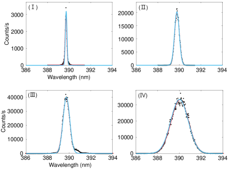
Figure 9: Simulated frequency spectra of pump pulses. The simulation results of spectra (blue lines) are obtained by using the Gaussian function to fit the experimental data (black dots and red lines) reported in Ref. [31]. The count rate also corresponds to Fig. 5 in Ref. [31]. The fitting parameters are shown in Table 6.

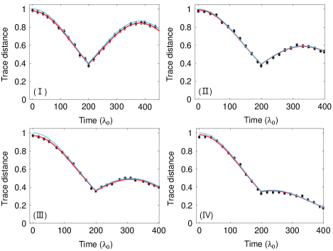
Figure 10: Simulations of trace distance under the four frequency correlation conditions (I)-(IV). The $\lambda_{0}$=780 nm denotes the effective path difference corresponding to Ref. [31]. We utilize the parameters listed in Table. 6 and substitute into Eq. (38) to simulate the trace distance of biphoton polarization states (blue lines). The simulated trace distance dynamics are highly consistent with the experimental trace distance dynamics (black dots and red lines) illustrated in Ref. [31]. The amounts of non-Markovianity evaluated by Eq. (LABEL:BLPnonMK) are: (I) $\mathcal{N_{\rm BLP}}=0.46$, (II) $\mathcal{N_{\rm BLP}}=0.20$, (III) $\mathcal{N_{\rm BLP}}=0.13$, and (IV) $\mathcal{N_{\rm BLP}}=0.01$.

A.2 Simulation method

To objectively compare our results with the conclusion of Laine et al. [32] and Liu et al. [31], we systematically exploit the experimental data reported in Ref. [31] to determine the Fourier transform of the joint frequency distribution, $G(\tau_{1},\tau_{2})$ (III.1.2), required to construct the process matrices $\chi^{\delta}_{t}$ (16) and $\chi^{\prime}_{t}$ (19). The steps of the simulation method are detailed as follows.

First, we use the following function:

$$f_{1}(x)=\tilde{X}{\rm exp}[-\tilde{Y}x^{2}],$$ (39)

to fit the experimental data of trace distance reported in Ref. [31] when the quartz plate in spatial mode 1 (QP1) is active. Thus, we can find the parameters $\tilde{X}$ and $\tilde{Y}$. The parameter $\tilde{Y}$ is obviously equal to $\Delta n^{2}C/2$ in Eq. (38).

Second, when the quartz plate in spatial mode 2 (QP2) is active, we use the function:

$$f_{2}(x)\!=\!\!\tilde{X}\!{\rm exp}[-\!\tilde{Y}\!(199^{2}\!\!+\!\!(x-\!199)^{2}\!\!-\!2|K|199(x-199))],$$ (40)

to fit the experimental data. Since $\tilde{X}$ and $\tilde{Y}$ are obtained from the first fitting step, the frequency correlation $K$ can be determined by the present fitting step.

Third, we use the following Gaussian function:

$$f_{3}(x)=\frac{1}{\sqrt{2\pi}\sigma_{0}}\text{exp}\left[-\frac{(x-\omega_{0})^{2}}{2\sigma_{0}^{2}}\right],$$ (41)

to fit the experimental data of the frequency spectra of pump pulses shown in Ref. [31]. From this fitting procedure, we can obtain the frequency center, $\omega_{0}$, and standard deviation, $\sigma_{0}$, of pump pulse spectra. According to the Gaussian distribution, we convert standard deviation to FWHM using $\delta=\sigma_{0}\sqrt{8\rm ln2}$, where $\delta$ is FWHM (full width at half maximum) of pump pulse spectra. The fitting parameters are shown in Table 6. To compare our simulating results with the experimental outcomes, they are depicted together in Fig. 9. As illustrated, the simulated spectra are highly consistent with the results reported in Ref. [31].

Fourth, to determine the unknown parameters $\Delta n$ and $C$, we utilize the numerical values in the third step and make an assumption about the frequency spectra of the single photon created by SPDC. That is, we assume that FWHM of the frequency spectrum of the single photon generated by SPDC is two times broader than that of the pump pulse, and the frequency spectrum of the single photon satisfies Gaussian distribution. Consequently, we obtain an estimate of frequency variance of the single photon created by SPDC through $C=(2\delta/\sqrt{8\rm ln2})^{2}$, in accordance with the Gaussian distribution. The rest unknown parameter $\Delta n$ can be acquired easily by evaluating $\tilde{Y}=\Delta n^{2}C/2$.

A.3 Process matrices

All parameters we obtained through the experimental data in Ref. [31] are listed in Table. 6. They are then used to construct the process matrices $\chi^{\delta}_{t}$ (16) and $\chi^{\prime}_{t}$ (19), and by which the time evolution of trace distance of $\ket{\phi^{+}}$ and $\ket{\phi^{-}}$ can be obtained as well. Finally, we simulate the trace distance under the four different conditions (I)-(IV) [see Eq. (III.2.2)] by the fitting parameters we obtained. The corresponding results are shown in Fig. 10. As shown, our simulations almost reproduce the results reported in Ref. [31]. A very small mismatch of the quantities of $\mathcal{N_{\rm BLP}}$ between the simulations and the measure reported in Ref. [31] is due to the error in the fitting procedure. Thus, we conclude that the underlying process matrices $\chi^{\delta}_{t}$ (16) and $\chi^{\prime}_{t}$ (19) are faithfully constructed from the experimental data shown in Ref. [31].

References

- [1] R. P. Feynman and F. L. Vernon, The theory of a general quantum system interacting with a linear dissipative system, Ann. Phys. (N.Y.) 24, 118 (1963).
- [2] F. Shibata, Y. Takahashi, and N. Hashitsume, A generalized stochastic Liouville equation. Non-Markovian versus memoryless master equations, J. Stat. Phys. 17, 171 (1977).
- [3] K. Kraus, States, Effects, and Operations: Fundamental Notions of Quantum Theory (Springer-Verlag, Berlin, Heidelberg, 1983).
- [4] H.-P. Breuer and F. Petruccione, The Theory of Open Quantum Systems (Oxford University Press, New York, 2002).
- [5] Y.-N. Chen, G.-Y. Chen, Y.-Y. Liao, N. Lambert, and F. Nori, Detecting non-Markovian plasmonic band gaps in quantum dots using electron transport, Phys. Rev. B 79, 245312 (2009).
- [6] W.-M. Zhang, P.-Y. Lo, H.-N. Xiong, M. W.-Y. Tu, and F. Nori, General non-Markovian dynamics of open quantum systems, Phys. Rev. Lett. 109, 170402 (2012).
- [7] X. Yin, J. Ma, X. G. Wang, and F. Nori, Spin squeezing under non-Markovian channels by the hierarchy equation method, Phys. Rev. A 86, 012308 (2012).
- [8] D. Chruściński and S. Maniscalco, Degree of non-Markovianity of quantum evolution, Phys. Rev. Lett. 112, 120404 (2014).
- [9] H.-B. Chen, J.-Y. Lien, G.-Y. Chen, and Y.-N. Chen, Hierarchy of non-Markovianity and k-divisibility phase diagram of quantum processes in open systems, Phys. Rev. A 92, 042105 (2015).
- [10] H.-B. Chen, N. Lambert, Y.-C. Cheng, Y.-N. Chen, and F. Nori, Using non-Markovian measures to evaluate quantum master equations for photosynthesis, Sci. Rep. 5, 12753 (2015).
- [11] H.-N. Xiong, P.-Y. Lo, W.-M. Zhang, D. H. Feng, and F. Nori, Non-Markovian complexity in the quantum-to-classical transition, Sci. Rep. 5, 13353 (2015).
- [12] Breuer, H., Laine, E., Piilo, J., Vacchini, B., Colloquium: Non-Markovian dynamics in open quantum systems, Rev. Mod. Phys. 88, 021001 (2016).
- [13] D. F. Urrego, J. Flrez, J. Svozilík, M. Nuez, and A. Valencia, Controlling non-Markovian dynamics using a light-based structured environment, Phys. Rev. A 98, 053862 (2018).
- [14] H.-B. Chen, P.-Y. Lo, C. Gneiting, J. Bae, Y.-N. Chen, and F. Nori, Quantifying the nonclassicality of pure dephasing, Nat. Comm. 10.1 (2019).
- [15] H.-P. Breuer, E.-M. Laine and J. Piilo, Measure for the degree of non-Markovian behavior of quantum processes in open systems, Phys. Rev. Lett. 103, 210401 (2009).
- [16] E.-M. Laine, J. Piilo and H.-P. Breuer, Measure for the non-Markovianity of quantum processes, Phys. Rev. A 81, 062115 (2010).
- [17] Á. Rivas, S. F. Huelga, and M. B. Plenio, Entanglement and non-Markovianity of quantum evolutions, Phys. Rev. Lett. 105, 050403 (2010).
- [18] S. Luo, S. Fu, and H. Song, Quantifying non-Markovianity via correlations, Phys. Rev. A 86, 044101 (2012).
- [19] H.-P. Breuer, Foundations and measures of quantum non-Markovianity, J. Phys. B 45, 154001 (2012).
- [20] Á. Rivas, S. F. Huelga, and M. B. Plenio, Quantum non-Markovianity: Characterization, quantification and detection, Rep. Prog. Phys. 77, 094001 (2014).
- [21] Guarnieri, G., Smirne, A., Vacchini, B., Quantum regression theorem and non-Markovianity of quantum dynamics, Phys. Rev. A. 90, 022110 (2014).
- [22] H.-P. Breuer, E.-M. Laine, J. Piilo, and B. Vacchini, Colloquium: Non-Markovian dynamics in open quantum systems, Rev. Mod. Phys. 88, 021002 (2016).
- [23] S.-L. Chen, N. Lambert, C.-M. Li, A. Miranowicz, Y.-N. Chen, and F. Nori, Quantifying non-Markovianity with temporal steering, Phys. Rev. Lett. 116, 020503 (2016).
- [24] I. de Vega and D. Alonso, Dynamics of non-Markovian open quantum systems, Rev. Mod. Phys. 89, 015001 (2017).
- [25] Li, C.-F., Guo, G.-C., Piilo, J, Non-Markovian quantum dynamics: What does it mean?, EPL. 127, 50001 (2019).
- [26] K.-D. Wu, Z. Hou, G.-Y. Xiang, C.-F. Li, G.-C. Guo, D. Dong, and F. Nori, Detecting non-Markovianity via quantified coherence: Theory and experiments, npj Quant. Inf. 6, 55 (2020).
- [27] X.-M. Lu, X. Wang, and C. P. Sun, Quantum Fisher information flow and non-Markovian processes of open systems, npj Quant. Inf. 6, 55 (2020).
- [28] S. Lorenzo, F. Plastina, and M. Paternostro, Geometrical characterization of non-Markovianity, Phys. Rev. A 6, 55 (2013).
- [29] G. Torre, W. Roga, and F. Illuminati, Non-Markovianity of gaussian channels, Phys. Rev. Lett. 115, 070401 (2015).
- [30] Liu, B.-H., Li, L., Huang, Y.-F., Li, C.-F., Guo, G.-C., Laine, E.-M., Breuer, H.-P., Piilo, J., Experimental control of the transition from Markovian to non-Markovian dynamics of open quantum systems, Nat. Phys. 7, 931 (2011).
- [31] Liu, B.-H., Cao, D.-Y., Huang, Y.-F., Li, C.-F., Guo, G.-C., Laine, E.-M., Breuer, H.-P., Piilo, J., Photonic realization of nonlocal memory effects and non-Markovian quantum probes, Sci. Rep. 3, 1781 (2013).
- [32] Laine, E.-M., Breuer, H.-P., Piilo, J., Li, C.-F., Guo, G.-C., Nonlocal memory effects in the dynamics of open quantum systems, Phys. Rev. Lett. 108, 210402 (2012).
- [33] Chruściński, D. and Pascazio, S., A brief history of the GKLS equation, Open Syst. Inf. Dyn. 24, 174001 (2017).
- [34] Lindblad, G., On the generators of quantum dynamical semigroups, Commun. Math. Phys. 48, 119 (1976).
- [35] Gorini, V., Kossakowski, A., Sudarshan, E., Completely positive dynamical semigroups of N-level systems, Math. Phys. 17, 821 (1976).
- [36] Kuo, C.-C., Chen, S.-H., Lee, W.-T., Chen, H.-M., Lu, H., Li, C.-M., Quantum process capability, Sci. Rep. 9, 20316 (2019).
- [37] Wang, K.-H., Chen, S.-H., Lin, Y.-C., Li, C.-M., Non-Markovianity of photon dynamics in a birefringent crystal, Phys. Rev. A. 98, 043850 (2018).
- [38] Nielsen, M. A. and Chuang, I. L. Quantum Computation and Quantum Information (Cambridge University Press, U.K., 2000).
- [39] Breuer, H.-P., Petruccione, F. and others The theory of open quantum systems (Oxford University Press on Demand, 2002).
- [40] Johan Löfberg, YALMIP: a toolbox for modeling and optimization in MATLAB®, CACSD. 10, 1109 (2004).
- [41] Toh, K.-C., Todd, M. J., Tütüncü, R. H., SDPT3–A Matlab software package for semidefinite-quadratic-linear programming in Matlab®, version 4.0, Handbook on Senidefinite. 10, 1007 (2012).
- [42] B. M. Terhal and G. Burkard, Fault-tolerant quantum computation for local non-Markovian noise, Phys. Rev. A 71, 012336 (2005).
- [43] D. Aharonov, A. Kitaev, and J. Preskill, Fault-tolerant quantum computation with long-range correlated noise, Phys. Rev. Lett. 96, 050504 (2006).
- [44] R. Takagi and B. Regula, General Resource Theories in Quantum Mechanics and Beyond: Operational Characterization via Discrimination Tasks, Phys. Rev. X 9, 031053 (2019).