Single-qubit loss-tolerant quantum position verification protocol secure against entangled attackers

Abstract

Protocols for quantum position verification (QPV) which combine classical and quantum information are insecure in the presence of loss. We study the exact loss-tolerance of the most popular protocol for QPV, which is based on BB84 states, and generalizations of this protocol. By bounding the winning probabilities of a variant of the monogamy-of-entanglement game using semidefinite programming (SDP), we find tight bounds for the relation between loss and error for these extended non-local games.

These new bounds enable the usage of QPV protocols using more-realistic experimental parameters. We show how these results transfer to the variant protocol which combines $n$ bits of classical information with a single qubit, thereby exhibiting a protocol secure against a linear amount of entanglement (in the classical information $n$) even in the presence of a moderate amount of photon loss. Moreover, this protocol stays secure even if the photon encoding the qubit travels arbitrarily slow in an optical fiber. We also extend this analysis to the case of more than two bases, showing even stronger loss-tolerance for that case.

Finally, since our semi-definite program bounds a monogamy-of-entanglement game, we describe how they can also be applied to improve the analysis of one-sided device-independent QKD protocols.

1 Introduction

Position-based cryptography (PBC), initially introduced by Chandran, Goyal, Moriarty and Ostrovsky [CGMO09], aims to allow a party to use its geographical location as a credential to implement various cryptographic protocols. An important building block for PBC is so-called Position Verification (PV), where an untrusted prover $P$ wants to convince a set of verifiers $V_{0},\dots,V_{k}$ that she is at a certain position $r$. In [CGMO09] it was proven that no secure classical protocol for position verification can exist, since there exists a general attack based on copying classical information. Adrian Kent first studied PV protocols that use quantum information in 2002, originally named quantum tagging [AKB06, KMS11] and currently called Quantum Position Verification (QPV) in the literature.Due to the no-cloning theorem [WZ82], attacks based on simply copying information do not transfer to the quantum setting. Nevertheless, unconditionally secure QPV was proven to be impossible, with [BCF⁺14] showing that any QPV could be attacked with double-exponential entanglement, which was later improved to exponential entanglement [BK11].

On the other side, it is possible to prove a linear lower bound for the amount of entanglement [BK11, TFKW13] – an exponential gap. Still, the extreme inefficiency of the general attack left the possibility open that QPV could be shown secure if we consider attackers that are bounded in some (realistic) way. Ideally that would mean a protocol which requires an exponential amount of entanglement to attack, but any provable gap between the hardness of executing the protocol versus breaking the protocol could be interesting. This possibility created the opportunity for many interesting follow-up work, showing security under model assumptions such as finding clever polynomial attacks to proposed protocols [LL11, CL15, Spe16a, Dol19, DC22, GC19, CM22] and analyzing security in other models, such as the random oracle model [Unr14, LLQ21, GLW16].

Particularly interesting here is the recent work by Liu, Liu, and Qian [LLQ21], which surprisingly shows that classical communication suffices to construct a secure protocol – immediately solving the issue of transmission loss. Despite this protocol being a great theoretical breakthrough, there are some downsides which make it unappealing to implement in the near future. A minor theoretical downside is that this proposed protocol is secure only under computational assumptions, and additionally requires the random oracle model to be secure against any entanglement. The larger practical downside is that the honest prover in [LLQ21]’s protocol requires a large quantum computer to execute the protocol’s steps – instead of manipulating and measuring single qubits as in most other protocols we’re considering.

One of the simplest and best-studied QPV protocols, which constitutes the basis of this work, is based on BB84 states, which we will denote $\mathrm{QPV}_{\mathrm{BB84}}$. This protocol was initially introduced in [KMS11] and later on proved secure against unentangled adversaries in [BCF⁺14], with parallel repetition shown in [TFKW13]. The protocol, explained in detail below, consists of one verifier ($V_{0}$) sending a BB84 state to the prover and the other verifier ($V_{1}$) sending a classical bit describing in which basis the prover has to measure, either the computational basis or the Hadamard basis. The prover then has to broadcast the measurement outcome to both verifiers, with all communication happening at the speed of light. This protocol can be attacked by attackers that share a single EPR pair. However, by encoding the basis information in several longer classical strings $x,y\in\{0,1\}^{n}$ that have to be combined in some way (i.e., the basis is given by $f(x,y)$ for some function $f$) it is possible to construct a single-qubit protocol, $\mathrm{QPV}_{\mathrm{BB84}}^{f}$, for which the quantum effort to break it grows with the amount of classical information that an honest party would use. This type of extension was already considered by Kent, Munro, and Spiller [KMS11] for a slightly different protocol, and analyzed more in-depth by Buhrman, Fehr, Schaffner, and Speelman [BFSS13], with a linear lower bound shown by Bluhm, Christandl, and Speelman [BCS22].(Also see [JKPPG22] for a related lower bound for a slightly different protocol which combines quantum and classical communication.) The ability to enhance security by adding classical information makes the functional version of $\mathrm{QPV_{BB84}}$ an appealing candidate for future use.

However, applying QPV experimentally encounters implementation problems, of which two are large enough that they force us to redesign our protocols. Whereas the transmission of classical information without loss at the speed of light is technologically feasible, e.g. via radio waves, the quantum counterpart faces obstacles. Firstly, most QPV protocols require the quantum information to be transmitted at the speed of light in vacuum, but the speed of light in optical fibers, a medium which would be necessary for many practical scenarios, is significantly lower than in vacuum. Secondly, a sizable fraction of photons is lost in transmission in practice. For this loss problem, we can distinguish two recent approaches. The first of which is to create protocols which are secure against any amount of loss, which we can call fully loss-tolerant protocols. This type of protocol was first introduced by Lim, Xu, Siopsis, Chitambar, Evans, and Qi [LXS⁺16], based on ideas from device-independent QKD. New examples and further analyses of fully loss-tolerant protocols were given by Allerstorfer, Buhrman, Speelman, and Verduyn Lunel [ABSV21, ABSL22]. These protocols could be excellent realistic candidates for an implementation of QPV, but in the longer term they have two shortcomings: they are not secure against much entanglement – [ABSL22] for instance show that if security against unbounded loss is required, this is unavoidable – and they require fast transmission of quantum information.

In this work we therefore advance another approach, which involves bounding the exact combination of loss rate and error rate that an attacker can achieve, thereby constructing what we may call partially loss-tolerant protocols. The first published example of this is given by Qi and Siopsis [QS15], who propose extending the $\mathrm{QPV_{BB84}}$ protocol to more bases to give some loss-tolerance, a proposal which was independently made by Buhrman, Schaffner, Speelman, and Zbinden (available as [Spe16b, Chapter 5]).

One might wonder: because it’s desirable to create a protocol which can tolerate a certain level of measurement error, and we are only secure against limited loss anyway, why it is not possible to see photon loss as merely another source of error? The answer is that it is very beneficial to treat these parameters separately because the numbers involved are entirely different. The basic $\mathrm{QPV_{BB84}}$ protocol has a perfect attack, which is possible by claiming a ‘loss’ 50% of the time. However, the best non-lossy attack has error 0.15. This means that an experimental set-up which has a loss of 49% could conceivably enable secure QPV, even though that clearly could never be good enough if the lost photons are counted as error. For different protocols, this difference in allowed parameters can be even larger.

In this paper, we study the security of the $\mathrm{QPV}_{\mathrm{BB84}}$  protocol in the lossy case, for attackers that do not pre-share entanglement, but that are allowed to perform local operations and a single simultaneous round of quantum communication (LOBQC) [GC19]. The best bounds for the non-lossy version of this protocol (for attackers that are allowed a round of quantum communication) come through reducing them to a monogamy-of-entanglement game [TFKW13] – we extend this game to include a third ‘loss’ response. Via Semidefinite Programming (SDP), we can then tightly bound the game’s winning probability, and therefore $\mathrm{QPV}_{\mathrm{BB84}}$’s security under photon loss, showing that a naive mixture of the extremal strategies turns out to give the optimal combination of error and response rate for the attackers. This is a three-player game involving two players, who have complete freedom, and a referee who performs a fixed measurement for every input. It is well-known how to analyze two-party scenarios using SDP relaxations, but extending these methods to three-party scenarios presents an obstacle. To obtain SDP bounds, we combine the NPA hierarchy [NPA08] with extra inequalities we derive from the relation between the referee’s measurements – the way these inequalities enable us to tackle a three-player problem using SDPs might be of independent interest.

Importantly, we are able to also show that these results can be adapted to show bounds for the lossy version of $\mathrm{QPV}_{\mathrm{BB84}}^{f}$. We do this by defining a new relaxation of our earlier SDP, which holds for the unentangled case, and show that the numerical bounds for this new SDP can be used to reprove a key lemma in [BCS22] for the case of our protocol. For instance, if the measurement error is very low, our results show that the single-qubit protocol $\mathrm{QPV}_{\mathrm{BB84}}^{f}$  remains secure against attackers that share an amount of entanglement that is sublinear in the amount of classical bits, even when only, e.g., $51\%$ of the photons arrive at the honest party. The security proof even goes through in the case that the transmission of quantum information is slow, as long as classical information can be transmitted fast.

Moreover, we extend the $\mathrm{QPV}_{\mathrm{BB84}}$  protocol where $V_{0}$ and $V_{1}$ agree on a qubit encoded in $m$ possible different bases over the whole Bloch sphere, a similar extension was proposed in [QS15], see below for the differences. Via SDP characterization, although tightness is not guaranteed for $m\geq 3$ in our results, we show that the new protocol becomes more resilient against photon loss when $m$ increases. Again, we are able to show this also holds for the extension to the protocol which lets the basis be determined by more-complicated classical information $\mathrm{QPV}^{\eta,f}_{m_{\theta\varphi}}$. For instance, for $m=5$, if the measurement error is very small the protocol remains secure against attackers sharing less than roughly $\frac{n}{2}$ EPR pairs, even if almost $70\%$ of the photons are lost for the honest parties.

The main result of this paper can be summarized as follows (see Theorems 3.12 and 5.7 for a formal version):

Theorem 1.1.

(Informal). If some attackers pre-share a linear amount (in the size of the classical information) of qubits before the $\mathrm{QPV}_{\mathrm{BB84}}^{\eta,f}$/ $\mathrm{QPV}^{\eta,f}_{m_{\theta\varphi}}$ protocol and if they respond with probability $\eta$, then the probability that they do not answer correctly is strictly larger than a numerical bound, which is a function of $\eta$. Therefore, if an honest prover, for which qubits arrive with probability $\eta$, has lower error probability, the protocol is correct and secure.

Our results also provide improved upper bounds for the probability of winning some concrete monogamy-of-entanglement (MoE) games [TFKW13], which encode attacks of QPV protocols. Finally, we apply our technique proofs to prove security of one-sided device-independent quantum key distribution (DIQKD) BB84 [BB84] for a single round $n=1$, see below, with security under photon loss. However, the interesting case is the asymptotic behavior for arbitrary $n$, which we leave as an open question.

Comparison to earlier work.

Our work is directly related to the questions asked by Qi and Siopsis [QS15]. The most important difference between that work and ours, is that we are considering a more general security model. The attack analysis in [QS15] is based upon an assumption that attackers would immediately measure an incoming qubit using a projective measurement, and then communicate classically. By reducing to (extensions of) monogamy-of-entanglement games, we instead capture any quantum action of the attackers, including a round of quantum communication – it’s shown in [ABSL22] that this stronger security model can in fact make a difference in the security. Critically, this also means that our method of analysis extends to the case where a classical function is combined with a single qubit, and our results make it possible to also prove entanglement bounds, instead of just bounds against unentangled protocols. Finally, our results can be reapplied in other settings that can be described by a monogamy-of-entanglement game.

There are two other recent papers by Allerstorfer, Buhrman, Speelman, and Verduyn Lunel [ABSV21, ABSL22] that study the role of loss in quantum position verification. Those works provide many new results on the capabilities and limitations of fully loss-tolerant protocols.

Our work builds upon the (unpublished) results of Buhrman, Schaffner, Speelman, and Zbinden [Spe16b, Chapter 5]. That work took the initial step to bound QPV protocols in the lossy case using SDPs. However, its analysis was incomplete and numerically significantly less tight, e.g., its bounds on $\mathrm{QPV_{BB84}}$ were a factor two worse than the current work. Additionally, we significantly extend its applicability by extending the technique to also show entanglement bounds for the $\mathrm{QPV}_{\mathrm{BB84}}^{f}$  protocol [BFSS13, BCS22].

2 The $\mathrm{QPV}_{\mathrm{BB84}}^{\eta}$ protocol and its security under unentangled attackers

Proposed QPV protocols rely on both relativistic constraints in a $d$-dimensional Minkowski space-time $M^{(d,1)}$ and the laws of quantum mechanics. In the literature, e.g. [KMS11, BFSS13], the case $d=1$ is mostly found, i.e. verifying the position of $P$ in a line, since it makes the analysis easier and the main ideas generalize to higher dimensions. The most general setting for a 1-dimensional QPV protocol is the following: two verifiers $V_{0}$ and $V_{1}$, placed on the left and right of $P$, send quantum and classical messages to $P$ at the speed of light, and she has to pass a challenge and reply correctly to them at the speed of light as well. The verifiers are assumed to have perfect synchronized clocks and if any of them receives a wrong answer or the timing does not correspond with the time it would have taken for light to travel back from the honest prover, they abort the protocol. Moreover, the time consumed by the prover to perform the challenge (usually a quantum measurement or a classical computation, see below for a detailed example) is assumed to be negligible.

One of the protocols that has been studied the most is the $\mathrm{QPV_{BB84}}$ protocol, see below, originally introduced in [KMS11]. Here we introduce a variation of it where we consider that the quantum information sent through the quantum channel between $V_{0}$ and $P$ can be lost. In practice, a representative example of this will be photon loss in optical fibers. We also consider that an honest party is assumed to have error rate $p_{err}$, and thus will also respond with a wrong answer sometimes. This error can arise, for example, either from measurement errors or from noise in the quantum channel where the qubit is sent through. We define one round of the lossy-BB84 QPV protocol as follows:

Definition 2.1.

(A round of the $\mathrm{QPV}_{\mathrm{BB84}}^{\eta}$ protocol). Let $\eta$ be the transmission rate of the quantum channel, we define one round of the lossy-BB84 QPV protocol, denoted by $\mathrm{QPV}_{\mathrm{BB84}}^{\eta}$, as follows (see Fig. 1 for steps 2. and 3.):

1. $V_{0}$ and $V_{1}$ secretly agree on a random bit $z$ and a basis $x\in\{0,1\}=:\mathcal{X}$, i.e. the computational $(0)$ or the Hadamard $(1)$ basis. In addition, $V_{0}$ prepares the EPR pair $\left|\Omega\right\rangle=(\left|00\right\rangle+\left|11\right\rangle)/\sqrt{2}$.

2. $V_{0}$ sends one qubit $Q$ of $\left|{\Omega}\right\rangle$ to $P$, and $V_{1}$ sends $x$ to $P$, coordinating their times so that $Q$ and $x$ arrive at $P$ at the same time.

3. Immediately, $P$ measures $Q$ in the basis $x$ and broadcasts her outcome, either 0 or 1, to $V_{0}$ and $V_{1}$. If the photon is lost, she sends $\perp$. Therefore, the possible answers from $P$ are $a\in\{0,1,\perp\}$.

4. Let $a$ and $b$ denote answers that $V_{0}$ and $V_{1}$ receive, respectively. If

   1. both $a$ and $b$ arrive on time and $a=b$, and if

      • they equal $z$, the verifiers output ‘Correct’,

      • they equal $1-z$, the verifiers output ‘Wrong’,

      • they equal $\perp$, the verifiers output ‘No photon’,

   2. if either $a$ or $b$ do not arrive on time or $a\neq b$, the verifiers output ‘Abort’.

The protocol is run sequentially $r$ times. Let $r_{\textsc{C}}$, $r_{\textsc{W}}$, $r_{\textsc{N}}$ and $r_{\textsc{A}}$ denote the number of times that the verifiers output ‘Correct’, ‘Wrong’, ‘No photon’ and ‘Abort’, respectively, after the $r$ rounds. The verifiers accept the prover’s location if the answers they receive match with $\eta$ and $p_{err}$ and they do not receive any different or delayed answers, i.e. if

$$\begin{split}r_{\textsc{C}}&\approx r\eta(1-p_{err}),\hskip 42.67912ptr_{\textsc{W}}\approx r\eta(1-p_{err}),\\ r_{\textsc{N}}&\approx r(1-\eta),\hskip 62.59596ptr_{\textsc{A}}=0.\end{split}$$ (1)

The symbols $\approx$ are due to the fact that in an implementation the above values would only be reached for $r\to\infty$. Notice that the verifiers remain strict with $r_{\textsc{A}}$, since an honest party would never send different answers and using current technology, her answers will arrive on time.

The $\mathrm{QPV}_{\mathrm{BB84}}$  protocol is recovered for $\eta=1$ and $p_{err}=0$. The above description of one round of the protocol corresponds to the purified version of the originally stated $\mathrm{QPV}_{\mathrm{BB84}}$  (for $\eta=1$). Notice that sending a single qubit $z$ in the basis $x$, as in the original version, instead of a qubit from an EPR pair, is completely equivalent to the above description. When $V_{0}$ measures $Q$ in the basis $x$, obtaining the random bit $z$, the reduced state sent to $P$ is given by $H^{x}\left|z\right\rangle$, where $H$ is the Hadamard matrix, and the original version is recovered. We will use the purified version in the analysis, because the security proofs are easier (in particular, it makes it easy to delay the choice of basis $x$ to a later point in time, which makes it clear that the attackers’ actions are independent of the basis choice).

Figure 1: Steps 2. and 3. of the $\mathrm{QPV}_{\mathrm{BB84}}^{\eta}$  protocol, where straight lines represent classical information and undulated lines represent quantum information. Image reproduced from [BCS22] with permission.

Whereas it is well-known that unlimited attackers can always successfully break any QPV protocol [BCF⁺14], the proof of the security of the $\mathrm{QPV_{BB84}}$ protocol under attackers that do not pre-share entanglement [BCF⁺14] opened a branch of study. The most general attack to a 1-dimensional QPV protocol is to place an adversary between $V_{0}$ and the prover, which we will call Alice, and another adversary between the prover and $V_{1}$, which we will call Bob. It is easy to see that having more than two adversaries in a 1-dimensional setting does not improve an attack. We now describe a general attack for attackers that do not pre-share entanglement.

Attack 2.2.

The most general attack to $\mathrm{QPV}_{\mathrm{BB84}}^{\eta}$, under the restriction that the attackers do not pre-share entanglement and are allowed to perform local operations and quantum communication (LOQC), consists of:

1. Alice intercepts the qubit $Q$ and applies an arbitrary quantum operation to it, and possibly some ancillary systems she possesses, ending up with the state $\rho$. She keeps a part of it and sends the other to Bob. On the other side, Bob intercepts $x$, copies it and sends the copy to Alice. Since they share no entanglement, any quantum operation that Bob could perform as a function of $x$ can be included in Alice’s operation (see e.g., [BCF⁺14, TFKW13]).

2. Each party performs a POVM $\{A^{x}_{a}\}$ and $\{B^{x}_{b}\}$, respectively, to the state $\rho$ and they send an answer $a,b\in\{0,1,\perp\}$ to their corresponding verifier.

The loss of quantum messages can be taken as an advantage from the point of view of the attackers. For example, assume that under the execution of the protocol the honest parties expect that half of the photons (or more) are lost in the transmission, i.e., $\eta\leq\frac{1}{2}$, but the attackers are able to receive all photons (since they can position themselves closer to the verifiers). Then the attacker Alice could make a random guess $\tilde{x}$ for $x$, measure the qubit $Q$ in the $\tilde{x}$ basis and broadcast the outcome and $\tilde{x}$ to fellow attacker Bob. After 1-round of simultaneous communication with Bob, they both know if the guess was correct. If so, they send the outcome to the verifiers, otherwise, they claim no photon arrived. Notice that Alice’s basis guess will be correct half of the time and therefore, the attackers can respond correctly half of the time, which is the expected ratio of transmission. We call this strategy the uniform strategy, and we denote it by $\mathbf{S}_{MoE-u}^{\eta=1/2}$, see below.

The tuple $\{\rho,A^{x}_{a},B^{x}_{b}\}_{x,a,b}$ will be called a non-entangled (NE) strategy. The probabilities that the verifiers, after the attackers’ actions (for the random variable $\textsc{V}_{\textsc{AB}}$) record correct, wrong, no photon and different answers (the verifiers ‘Abort’ in such a case) are thus, respectively, given by

$$\mathbb{P}[\textsc{V}_{\textsc{AB}}=\textsc{Correct}] =\frac{1}{\lvert\mathcal{X}\rvert}\sum_{a\in\{0,1\},x\in\mathcal{X}}\mathrm{Tr}\left[\rho V^{x}_{a}\otimes A^{x}_{a}\otimes B^{x}_{a}\right],$$ (2)

$$\mathbb{P}[\textsc{V}_{\textsc{AB}}=\textsc{Wrong}] =\frac{1}{\lvert\mathcal{X}\rvert}\sum_{a\in\{0,1\},x\in\mathcal{X}}\mathrm{Tr}\left[\rho V^{x}_{a}\otimes A^{x}_{1-a}\otimes B^{x}_{1-a}\right],$$ (3)

$$\mathbb{P}[\textsc{V}_{\textsc{AB}}=\textsc{No photon}] =\frac{1}{\lvert\mathcal{X}\rvert}\sum_{x\in\mathcal{X}}\mathrm{Tr}\left[\rho\mathbb{I}\otimes A^{x}_{\perp}\otimes B^{x}_{\perp}\right],$$ (4)

$$\mathbb{P}[\textsc{V}_{\textsc{AB}}=\textsc{Abort}] =\frac{1}{\lvert\mathcal{X}\rvert}\sum_{a\neq b\in\{0,1,\perp\},x\in\mathcal{X}}\mathrm{Tr}\left[\rho\mathbb{I}\otimes A^{x}_{a}\otimes B^{x}_{b}\right].$$ (5)

Through this paper, $\mathbb{P}[*]$ will denote the probability of event $*$. Similarly, we will consider the random variable $\textsc{V}_{\textsc{P}}$ if the actions are performed by the prover. We say that an attack to a round of the protocol is successful if the following are fulfilled:

$$\begin{split}&\mathbb{P}[\textsc{V}_{\textsc{AB}}=\textsc{Correct}]=\eta(1-p_{err}),\hskip 42.67912pt\mathbb{P}[\textsc{V}_{\textsc{AB}}=\textsc{Wrong}]=\eta p_{err},\\ &\mathbb{P}[\textsc{V}_{\textsc{AB}}=\textsc{No photon}]=1-\eta,\hskip 48.36958pt\mathbb{P}[\textsc{V}_{\textsc{AB}}=\textsc{Abort}]=0.\end{split}$$ (6)

A single round attack to $\mathrm{QPV}_{\mathrm{BB84}}^{\eta,f}$  for $\eta=1$ can be identified with a so-called monogamy-of-entanglement (MoE) game, introduced by Tomamichel, Fehr, Kaniewski and Wehner in [TFKW13], formalized below in Definition 2.3 and generalized by Johnston, Mittal, Russo, and Watrous [JMRW16]. The authors of [TFKW13] showed that the optimal probability that the attackers are correct in one round of the $\mathrm{QPV}_{\mathrm{BB84}}$ protocol is $1-\cos^{2}\pi/8$. Moreover, they show strong parallel repetition, i.e. if $\mathrm{QPV}_{\mathrm{BB84}}$ is executed $n$ times in parallel, the probability that the attackers are correct is at most $(1-\cos^{2}\pi/8)^{n}$.

Here we consider an extension of a MoE game, which we will call lossy MoE game, that will capture a round attack of $\mathrm{QPV}_{\mathrm{BB84}}^{\eta}$.

Definition 2.3.

A lossy monogamy-of-entanglement game with parameter $\eta\in[0,1]$ consists of a finite dimensional Hilbert space $\mathcal{H}_{V}$, corresponding to party $V$, and a list of measurements $\{V_{v}^{x}\}_{v\in\mathcal{V}}$ on $\mathcal{H}_{V}$, indexed by $x\in\mathcal{X}$, where $\mathcal{V}$ and $\mathcal{X}$ are finite sets. Two collaborative parties, Alice and Bob, with associated Hilbert spaces $\mathcal{H}_{A}$ and $\mathcal{H}_{B}$, respectively, prepare an arbitrary quantum state $\rho_{VAB}$ and send $\rho_{V}$ to $V$, holding on $\rho_{A}$ and $\rho_{B}$, respectively. $V$ chooses $x\in\mathcal{X}$ uniformly at random and measures $\rho_{V}$ using $\{V_{v}^{x}\}$ to obtain the measurement outcome $v$. Then she announces $x$ to Alice and Bob. The collaborative parties make a guess of $v$ and they win the game if and only if both either guess $v$ correctly or their strategy, see below, is such that (8) is fulfilled.

A MoE game as in [TFKW13] is recovered for $\eta=1$. The interpretation of the lossy MoE game compared with the original MoE game is that the two collaborative parties have the ‘extra power’ of answering ‘$\perp$’ which can be seen as them saying ‘I do not know’ with probability $1-\eta$.

Definition 2.4.

A strategy $\mathbf{S}_{MoE}^{\eta}$ for a lossy monogamy-of-entanglement game is a tuple

$$\mathbf{S}^{\eta}_{MoE}=\{\rho_{VAB},A_{v}^{x},B_{v}^{x}\}_{v\in\mathcal{V}\cup\{\perp\},x\in\mathcal{X}},$$ (7)

where $\rho_{VAB}$ is a density operator on $\mathcal{H}_{V}\otimes\mathcal{H}_{A}\otimes\mathcal{H}_{B}$ and for all $x\in\mathcal{X}$, $\{A_{v}^{x}\}_{v\in\mathcal{V}\cup\{\perp\}}$ and $\{B_{v}^{x}\}_{v\in\mathcal{V}\cup\{\perp\}}$ are POVMs on $\mathcal{H}_{A}$ and $\mathcal{H}_{B}$, respectively, such that

$$\frac{1}{\lvert\mathcal{X}\rvert}\sum_{x\in\mathcal{X}}\mathrm{Tr}\left[\rho_{VAB}\mathbb{I}\otimes A^{x}_{\perp}\otimes B^{x}_{\perp}\right]=1-\eta.$$ (8)

In [TFKW13] it is shown that any strategy can be purified in the sense that, enlarging the corresponding Hilbert spaces if necessary, $\rho_{VAB}=\left|\psi\rangle\langle\psi\right|$ is a pure state for $\left|\psi\right\rangle\in\mathcal{H}_{V}\otimes\mathcal{H}_{A}\otimes\mathcal{H}_{B}$ and $\{A_{v}^{x}\}$, $\{B_{v}^{x}\}$ are projective measurements. Therefore, unless it is explicitly specified, from now on we will consider any strategy $\mathbf{S}^{\eta}_{MoE}$, with $\mathbf{S}^{\eta}_{MoE}$ pure. A MoE game can be associated with an attack to the $\mathrm{QPV_{BB84}}$ protocol in the sense that having a strategy to break the protocol implies having a strategy for the MoE game [TFKW13, Section 5]. In a similar manner, it follows that having a $\mathbf{S}^{\eta}_{MoE}$ strategy implies having a NE strategy for $\mathrm{QPV}_{\mathrm{BB84}}^{\eta}$. The idea is that in item 2. in the attack described as Attack 2.2, the attackers start with a tripartite state shared among the verifier, Alice and Bob and their task is to correctly guess the measurement outcome of the measurement which is performed on the verifier’ register. In the $\mathrm{QPV}_{\mathrm{BB84}}$ protocol case, $V$ corresponds to the verifiers with associated Hilbert space $\mathcal{H}_{V}=\mathbb{C}^{2}$, with $\mathcal{X}=\{0,1\}$ and $\mathcal{V}=\{0,1\}$. The verifiers $V$ perform the collection of measurements

$$\{V_{0}^{x},V_{1}^{x}\}_{x\in\{0,1\}},$$ (9)

where $V_{0}^{x}=H^{x}\left|0\rangle\langle 0\right|H^{x}$ and $V_{1}^{x}=H^{x}\left|1\rangle\langle 1\right|H^{x}$, where $H$ is the Hadamard transformation, and the two collaborative parties, who correspond to the attackers, want to break the protocol by guessing the verifier’s outcome. The strategy $\mathbf{S}_{MoE-BB84}^{\eta=1}=\{\left|\psi\rangle\langle\psi\right|,A_{a}^{x}=\delta_{a0},B_{a}^{x}=\delta_{a0}\}$, where $\left|\psi\right\rangle=\cos\frac{\pi}{8}\left|0\right\rangle+\sin\frac{\pi}{8}\left|1\right\rangle$, gives the optimal probability of winning the MoE game (see discussion below) and thus the optimal probability of being correct attacking the $\mathrm{QPV}_{\mathrm{BB84}}$ protocol,

$$\mathbb{P}[\textsc{V}_{\textsc{AB}}=\textsc{Correct}]=\frac{1}{\lvert\mathcal{X}\rvert}\sum_{a,x}\mathrm{Tr}\left[\left|\psi\rangle\langle\psi\right|V^{x}_{a}\otimes A^{x}_{a}\otimes B^{x}_{a}\right]=1-\cos^{2}\frac{\pi}{8}.$$ (10)

This strategy also gives, using (6),

$$\mathbb{P}[\textsc{V}_{\textsc{AB}}=\textsc{Wrong}]=\cos^{2}\frac{\pi}{8},\hskip 28.45274pt\mathbb{P}[\textsc{V}_{\textsc{AB}}=\textsc{Abort}]=0.$$ (11)

Comparing it with (6), and considering that $\eta=1$, the attackers could successfully attack one round of the $\mathrm{QPV}_{\mathrm{BB84}}$ protocol if $p_{err}=\cos^{2}\frac{\pi}{8}$. Notice that if in a lossy MoE game the attackers actually ‘play’, meaning that they do not respond ‘$\perp$’, we have

$$\begin{split}&\mathbb{P}[\textsc{V}_{\textsc{AB}}=\textsc{Correct}\mid\textsc{V}_{\textsc{AB}}\neq\textsc{No photon}]+\mathbb{P}[\textsc{V}_{\textsc{AB}}=\textsc{Wrong}\mid\textsc{V}_{\textsc{AB}}\neq\textsc{No photon}]\\ &+\mathbb{P}[\textsc{V}_{\textsc{AB}}=\textsc{Abort}\mid\textsc{V}_{\textsc{AB}}\neq\textsc{No photon}]=1.\end{split}$$ (12)

In fact, since for QPV we impose $\mathbb{P}[\textsc{V}_{\textsc{AB}}=\textsc{Abort}]=0$, the above expression reduces to

$$\mathbb{P}[\textsc{V}_{\textsc{AB}}=\textsc{Correct}\mid\textsc{V}_{\textsc{AB}}\neq\textsc{No photon}]+\mathbb{P}[\textsc{V}_{\textsc{AB}}=\textsc{Wrong}\mid\textsc{V}_{\textsc{AB}}\neq\textsc{No photon}]=1.$$ (13)

We define the probability of winning, $p_{win}$ as the maximum probability of being correct conditioned on answering, i.e. $p_{win}:=\max\mathbb{P}[\textsc{V}_{\textsc{AB}}=\textsc{Correct}\mid\textsc{V}_{\textsc{AB}}\neq\textsc{No photon}]$. In fact, this corresponds to what in [TFKW13] is defined as the probability of winning the MoE game. Moreover, since for the BB84 MoE game it is always the case that $\textsc{V}_{\textsc{AB}}\neq\textsc{No photon}$, we have that the optimal probability of winning the game is

$$p_{win}=\mathbb{P}[\textsc{V}_{\textsc{AB}}=\textsc{Correct}\mid\textsc{V}_{\textsc{AB}}\neq\textsc{No photon}]=\mathbb{P}[\textsc{V}_{\textsc{AB}}=\textsc{Correct}]=1-\cos^{2}\frac{\pi}{8},$$ (14)

which is obtained using $\mathbf{S}_{MoE-BB84}^{\eta=1}$.

The security of the $\mathrm{QPV}_{\mathrm{BB84}}^{\eta}$ protocol relies on the probability that the attackers can win the lossy MoE game. The usage of Semidefinite Programming (SDP) techniques to bound non-local games was initiated by Cleve, Hoyer, Toner and Watrous [CHTW04] and Wehner [Weh06]. In order to apply these techniques, we take our security approach on the probability that the attackers can actually play the game without being caught, i.e., the probability that they can answer, $p_{ans}$,

$$p_{ans}=\mathbb{P}[\textsc{V}_{\textsc{AB}}=\textsc{Correct}]+\mathbb{P}[\textsc{V}_{\textsc{AB}}=\textsc{Wrong}]=\frac{1}{2}\sum_{x,a\in\{0,1\}}\left\langle\psi\right|A_{a}^{x}B_{a}^{x}\left|\psi\right\rangle,$$ (15)

where we used the following simplified notation: when clear from the context, tensor products, identities and $\psi$ will be omitted, e.g., $\left\langle\psi\right|V_{0}^{x}\otimes A_{1}^{x}\otimes B_{1}^{x}\left|\psi\right\rangle=\langle V_{0}^{x}A_{1}^{x}B_{1}^{x}\rangle$.

This probability of answer needs to restrict the probability that the attackers are wrong. The prover’s error $p_{err}$ is such that

$$\frac{\langle V_{0}^{x}A_{1}^{x}B_{1}^{x}\rangle}{\langle V_{0}^{x}(A_{0}^{x}+A_{1}^{x})(B_{0}^{x}+B_{1}^{x})\rangle}\leq p_{err},\hskip 28.45274pt\frac{\langle V_{1}^{x}A_{0}^{x}B_{0}^{x}\rangle}{\langle V_{1}^{x}(A_{0}^{x}+A_{1}^{x})(B_{0}^{x}+B_{1}^{x})\rangle}\leq p_{err},$$ (16)

where we impose that the error rate for both outputs 0 and 1 is upper bounded by the same amount for all inputs $x$.

Notice that if $p_{ans}=1$, the attackers can always attack the protocol without being caught. Using (15), the security of the protocol can be regarded as the maximum probability that the attackers can respond without being caught, and the protocol will be proven to be secure if the attackers cannot reproduce $p_{ans}\geq\eta$ for a given $p_{err}$, we formalize this idea in the following definition.

Definition 2.5.

We define the security region $SR$ of the $\mathrm{QPV}_{\mathrm{BB84}}^{\eta}$  protocol as the set of pairs $(p_{err},p_{ans})\in[0,1]\times[0,1]$ for which no strategy $\mathbf{S}^{\eta}_{MoE}$ (and thus no NE strategy) exists that breaks the $\mathrm{QPV}_{\mathrm{BB84}}^{\eta}$  protocol with the corresponding error and response rate. A subset of $SR$ will be denoted by $SSR$. We define the attackable region $AR$ as the complementary set of the $SR$. A subset of $AR$ will be denoted as $SAR$.

Therefore, our interest relies on maximizing expression (15) over all the strategies $\mathbf{S}^{\eta}_{MoE}$ to break the $\mathrm{QPV}_{\mathrm{BB84}}^{\eta}$  protocol. However, unlike the set of probabilities achievable by classical physics, the set of probabilities attainable by quantum mechanics, $\mathcal{Q}$, has uncountably many extremal points, see e.g. [BCP⁺14], and therefore it makes the optimization problem a tough task. On the positive side, in [NPA08], Navascués, Pironio and Acín (NPA) introduced a recursive way to construct subsets ${\mathcal{Q}_{\ell}\supset\mathcal{Q}_{\ell+1}\supset\mathcal{Q}}$ for all $\ell\in\mathbb{N}$ with the property that each of them can be tested using SDP and are such that $\cap_{\ell\in\mathbb{N}}\mathcal{Q}_{\ell}=\mathcal{Q}$.

For all $a,b\in\{0,1,\perp\}$ and all $x,x^{\prime}\in\{0,1\}$, the elements $\langle A_{a}^{x}B_{b}^{x^{\prime}}\rangle$ will appear in the maximization problem solvable via SDP, and they are bounded by linear constraints given by $\mathcal{Q}_{\ell}$, see Appendix A. In addition to these constraints, we impose the additional linear constraints derived from $\mathrm{QPV}_{\mathrm{BB84}}^{\eta}$, i.e., since in the protocol the verifiers abort if they receive different messages, from (5),

$$\langle A_{a}^{x}B_{b}^{x}\rangle=0\hskip 14.22636pt\forall a\neq b\in\{0,1,\perp\},\forall x\in\{0,1\},$$ (17)

and the prover subject to a measurement error $p_{err}$, see Proposition 2.6.

Proposition 2.6.

Let $a,b\in\{0,1\}$. For all $x,x^{\prime}\in\{0,1\}$, the terms $\langle A_{a}^{x}B_{b}^{x^{\prime}}\rangle$ can be bounded by $p_{err}$ by the following inequality:

$$\sum_{ab}(2-\|V_{a}^{x}+V_{b}^{x^{\prime}}\|)\langle A_{a}^{x}B_{b}^{x^{\prime}}\rangle\leq p_{err}\sum_{a}(\langle A_{a}^{x}B_{a}^{x}\rangle+\langle A_{a}^{x^{\prime}}B_{a}^{x^{\prime}}\rangle).$$ (18)

The proof is a particular case of the proof of Proposition 4.2.
The value of $p_{ans}$ in (15) can be therefore upper bounded by the SDP problem:

$$\boxed{\begin{split}&\max\frac{1}{2}\sum_{x,a\in\{0,1\}}\langle A_{a}^{x}B_{a}^{x}\rangle;\\ &\textrm{subject to: the linear constraints for }\mathbf{S}^{\eta}_{MoE}\in\mathcal{Q}_{\ell},\\ &\textrm{ \hskip 42.67912pt and equations \eqref{eq restriction error epsilon BB84} and \eqref{eq perr constraint sum ab BB84}}.\end{split}}$$ (19)

Where, abusing notation, we denoted $\mathbf{S}^{\eta}_{MoE}\in\mathcal{Q}_{\ell}$ meaning that the probabilities obtained from $\mathbf{S}^{\eta}_{MoE}$ belong to the set $\mathcal{Q}_{\ell}$. Fig. 2 shows the solution of the SDP (19) for different values of $p_{err}$ for the first and second level of the NPA hierarchy using the Ncpol2sdpa package [Wit15] in Python. The values above the solution for any given $p_{err}$ represent points where does not exist an attack such that $p_{ans}\geq\eta$ and therefore correspond to $SSR$, the area represented in light blue. The results plotted in Fig. 2 coincide with the tight bound of the winning probability of the MoE game attacking the $\mathrm{QPV_{BB84}}$ protocol, since $p_{ans}$ reaches 1 for $p_{err}=0.1464\simeq 1-\cos^{2}(\pi/8)$.

Proposition 2.7.

The function $p_{ans}(p_{err})$ for $p_{err}\in[0,1]$ obtained by the solution of (19) is monotonically increasing, i.e. if $p_{err}^{0}\leq p_{err}^{1}$, then $p_{ans}(p_{err}^{0})\leq p_{ans}(p_{err}^{1})$.

Proof.

It follows from the fact that $p_{ans}(p_{err}^{1})$ is obtained by an SDP which relaxation of the restrictions of the SDP providing $p_{ans}(p_{err}^{0})$. ∎

Informally, Proposition 2.7 assures that between two numerical solutions for different $p_{err}$ there are no ‘abrupt jumps’, more specifically, in Fig.  2, any solution between two plotted points cannot be grater than the point in the right.

Consider the strategy $\mathbf{S}_{MoE}^{mix}|_{p}$ given by the probabilistic mixture of playing the strategy $\mathbf{S}_{MoE-BB84}^{\eta=1}$ with probability $p$ and $\mathbf{S}_{MoE-u}^{\eta=1/2}$ with probability $1-p$, conditioned on answering. As long as $p_{ans}<1$, for each $p$, this mixture gives a unique pair of $(p_{err},p_{ans})$ (for $p_{ans}=1$, take the minimum $p_{err}$), and we equivalently denote $\mathbf{S}_{MoE}^{mix}|_{p}$ by the corresponding $(p_{err},p_{ans})$ as $\mathbf{S}_{MoE}^{mix}|_{(p_{err},p_{ans})}$. The values of $p_{ans}$ obtained by this strategy, see continuous line in Fig. 2, provide a region where the protocol is attackable, i.e. a $SAR$. Since the SSR obtained from the second level of the NPA hierarchy and the $SAR$ obtained from $\mathcal{S}_{EoM}^{mix}|_{p}$ are such that $SSR\cup SAR=[0,1]\times[0,1]$, up to infinitesimal precision, it means that they correspond to $SR$ and $AR$, respectively, i.e., the solutions of the SDP (19) for $\ell=2$ converge to the quantum value and are tight. This means that Fig. 2 represents a full characterization of the security of the $\mathrm{QPV}_{\mathrm{BB84}}^{\eta}$ protocol under photon loss with attackers that do not pre-share entanglement, and the light blue region encodes all the points $(p_{err},\eta)$ where the protocol is secure. The result is summarized as follows:

Result 2.8.

Given a transmission rate $\eta$ and a prover’s measurement device subject to a measurement error $p_{err}$, for attackers that do not pre-share entanglement but are allowed to perform $\mathrm{LOQC}$, there does not exist any better strategy to break the $\mathrm{QPV}_{\mathrm{BB84}}^{\eta}$ than the strategy $\mathbf{S}_{MoE}^{mix}|_{(p_{err},\eta)}$.

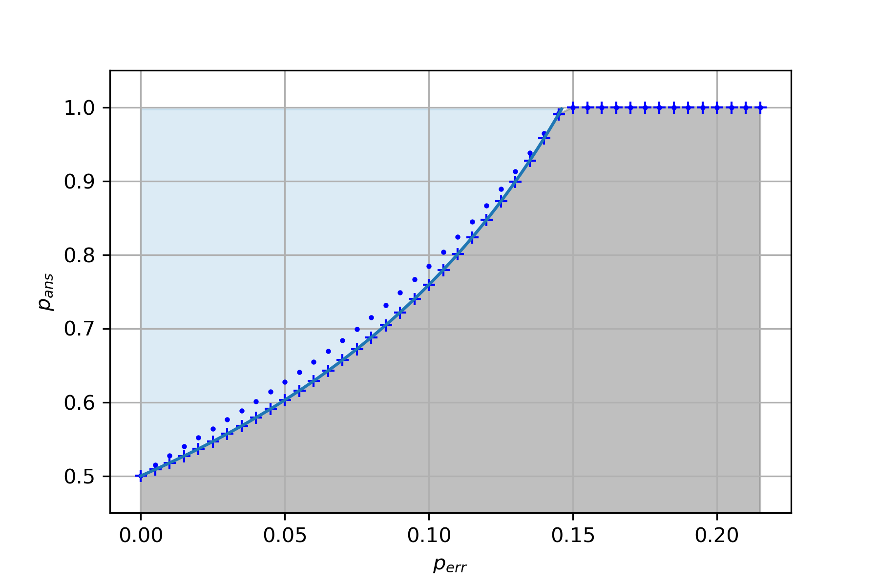
Figure 2: Solutions of the first, $\ell=1$, (blue dots) and second level, $\ell=2$, (blue pluses) of the NPA hierarchy for the SDP (19). The light blue and the gray area correspond to $SR$ and $AR$, respectively. The continuous line represents $\mathbf{S}_{MoE}^{mix}|_{p}$.

3 The $\mathrm{QPV}_{\mathrm{BB84}}^{\eta,f}$ protocol and its security under entangled attackers

In the previous section, we have shown security for the $\mathrm{QPV}_{\mathrm{BB84}}^{\eta}$ protocol. Our argument was restricted to attackers who do not pre-share entanglement, and it is well-known [KMS11] that such a protocol is broken with a single EPR pair. Recent work by Bluhm, Christandl and Speelman [BCS22], building on work by Buhrman, Fehr, Schaffner, and Speelman [BFSS13], has shown that when adding classical information to $\mathrm{QPV}_{\mathrm{BB84}}$, the $\mathrm{QPV}_{\mathrm{BB84}}^{f}$  protocol (see below), the protocol remains secure if the attackers hold less than $n/2-5$ qubits, making it secure against entangled attackers that hold an entangled state of smaller dimension. Recall that an attack on a QPV protocol can conceptually be split up into two rounds – the first in which the attackers hold part of the input and their pre-shared entangled state, and the second round in which the attackers have to respond to the closest verifier. The key to showing their result is by considering two possible joint states held by the attackers as a result of their first-round actions – one for an input where they have to measure the input qubit in the computational basis and one where they have to measure the qubit in the Hadamard basis. Then, these two states already have to be ‘far apart’ (even though Alice’s part does not depend on Bob’s input yet, and vice-versa), which by a counting argument makes it possible to obtain a bound on the size of the pre-shared state. In the spirit of applying an analogous counting argument to show security for the lossy case, we use the results of Section 2 to prove a lemma (Lemma 3.6) that allows us to apply a similar counting argument.

We define one round of the lossy-function-BB84 protocol as follows:

Definition 3.1.

(A round of the $\mathrm{QPV}_{\mathrm{BB84}}^{\eta,f}$ protocol). Let $n\in\mathbb{N}$, and consider a $2n$-bit boolean function $f:\{0,1\}^{n}\times\{0,1\}^{n}\to\{0,1\}$. We define one round of the lossy-function-BB84 protocol, denoted by $\mathrm{QPV}_{\mathrm{BB84}}^{\eta,f}$, as follows (see Fig. 3 for steps 2. and 3.):

1. $V_{0}$ and $V_{1}$ secretly agree on two random bit strings $x,y\in\{0,1\}^{n}$, which give a function value $f(x,y)\in\{0,1\}$. We will use function value 0 as denoting the computational basis and value 1 for the Hadamard basis. In addition, $V_{0}$ prepares the EPR pair $\left|\Omega\right\rangle=(\left|00\right\rangle+\left|11\right\rangle)/\sqrt{2}$.

2. $V_{0}$ sends one qubit $Q$ of $\left|\Omega\right\rangle$ and $x$ to $P$ and $V_{1}$ sends $y$ to $P$, coordinating their times so that $Q$, $x$ and $y$ arrive at $P$ at the same time. The verifiers are required to send the classical information at the speed of light, however, the quantum information can be sent arbitrarily slow .

3. Immediately, $P$ measures $Q$ in the basis $f(x,y)$ and broadcasts her outcome to $V_{0}$ and $V_{1}$. If the photon is lost, she sends $\perp$.

4. Let $a$ and $b$ denote answers that $V_{0}$ and $V_{1}$ receive, respectively. If

   1. both $a$ and $b$ arrive on time and $a=b$, and if

      • they are correct, the verifiers output ‘Correct’,

      • they are wrong, the verifiers output ‘Wrong’,

      • they are $\perp$, the verifiers output ‘No photon’,

   2. if either $a$ or $b$ do not arrive on time or $a\neq b$, the verifiers output ‘Abort’.

In the same way as for $\mathrm{QPV}_{\mathrm{BB84}}^{\eta}$, after $r$ rounds, the verifiers accept the prover’s location if they reproduce (1). Notice that $\mathrm{QPV}_{\mathrm{BB84}}^{f}$  corresponds to $\mathrm{QPV}_{\mathrm{BB84}}^{\eta,f}$  for $\eta=1$ and $p_{err}$=0.

Figure 3: Steps 2. and 3. of the $\mathrm{QPV}_{\mathrm{BB84}}^{\eta,f}$ protocol, where straight lines represent classical information and undulated lines represent quantum information. Image reproduced from [BCS22] with permission.

Consider a general attack to the $\mathrm{QPV}_{\mathrm{BB84}}^{\eta,f}$ protocol, where Alice and Bob take the same role as in Section 2, but in addition, they have quantum registers that are able to hold $q$ qubits each, which can be possibly entangled. Since they will intercept the qubit sent by the $V_{0}$, the joint system will consist of $2q+1$ qubits. We now describe a general attack with attackers who pre-share entanglement.

Attack 3.2.

A general attack for a round of the $\mathrm{QPV}_{\mathrm{BB84}}^{\eta,f}$ protocol consists of (the superscripts denote dependence on $x$ and $y$, correspondingly):

1. Alice intercepts the qubit $Q$ and applies an arbitrary quantum operation to it and to her qubits, possibly entangling them. She keeps part of the resulting state, $q$ qubits at most, and sends the rest to Bob. Since the qubit $Q$ can be sent arbitrarily slow by $V_{0}$ (the verifiers only time the classical information), this happens before Alice and Bob can intercept $x$ and $y$. At this stage, Alice, Bob, and $V_{0}$ share a quantum state $\left|\psi\right\rangle$ of $2q+1$ qubits.

2. Alice and Bob intercept $x$ and $y$, and apply a unitary $U_{A}^{x}$ and $U_{B}^{y}$ on their local registers, respectively. Alice sends a part of her local state and $x$ to Bob and, Bob sends a part of his local state and $y$ to Alice. Denote by $\rho^{xy}$ their joint state.

3. Each party performs a POVM $\{A^{xy}_{a}\}$ and $\{B^{xy}_{b}\}$, $a,b\in\{0,1,\perp\}$, on their registers and Alice sends her outcome $a$ to $V_{0}$ and Bob sends his outcome $b$ to $V_{1}$.

A $q$-qubit strategy [BCS22] for $\mathrm{QPV}_{\mathrm{BB84}}^{\eta,f}$ consists of a starting state $\left|\psi\right\rangle$, corresponding to the starting state to attack the $\mathrm{QPV}_{\mathrm{BB84}}^{\eta,f}$ protocol in step 1. before applying the unitary evolutions, unitaries $U_{A}^{x}$, $U_{B}^{y}$ and POVMs $\{A^{xy}_{a}\}$, $\{B^{xy}_{b}\}$, as described above. It can also be described by the tuple $\{\rho^{xy},A^{xy}_{a},B^{xy}_{b}\}_{x,y,a,b}$. The probabilities that the verifiers, after the attackers’ actions (for the random variable $\textsc{V}_{\textsc{AB}}$, as denoted above) record correct, wrong, no photon and different answers (the verifiers ‘Abort’ in such a case) are thus, respectively, given by

$$\begin{split}\mathbb{P}[\textsc{V}_{\textsc{AB}}=\textsc{Correct}]&=\frac{1}{2^{2n}}\sum_{a\in\{0,1\},x,y\in\{0,1\}^{n}}\mathrm{Tr}\left[\rho^{xy}V^{f(x,y)}_{a}\otimes A^{xy}_{a}\otimes B^{xy}_{a}\right],\\ \mathbb{P}[\textsc{V}_{\textsc{AB}}=\textsc{Wrong}]&=\frac{1}{2^{2n}}\sum_{a\in\{0,1\},x,y\in\{0,1\}^{n}}\mathrm{Tr}\left[\rho^{xy}V^{f(x,y)}_{a}\otimes A^{xy}_{1-a}\otimes B^{xy}_{1-a}\right],\\ \mathbb{P}[\textsc{V}_{\textsc{AB}}=\textsc{No photon}]&=\frac{1}{2^{2n}}\sum_{x,y\in\{0,1\}^{n}}\mathrm{Tr}\left[\rho^{xy}\mathbb{I}\otimes A^{xy}_{\perp}\otimes B^{xy}_{\perp}\right],\\ \mathbb{P}[\textsc{V}_{\textsc{AB}}=\textsc{Abort}]&=\frac{1}{2^{2n}}\sum_{a\neq b\in\{0,1,\perp\},x,y\in\{0,1\}^{n}}\mathrm{Tr}\left[\rho^{xy}\mathbb{I}\otimes A^{xy}_{a}\otimes B^{xy}_{b}\right].\end{split}$$ (20)

The criterion for a successful attack to a round of the protocol is the same as for $\mathrm{QPV}_{\mathrm{BB84}}^{\eta}$, i.e. (6) is fulfilled.

Our goal is to show that if the number of qubits that the attackers hold at the beginning of the protocol is linear, then given that they do not respond ‘$\perp$’, their probability of being correct is strictly less than the corresponding probability of the honest prover. To this end, we define a relaxation of the condition of being correct, and we consider $q$-qubit strategies which have a high chance that the verifiers record Correct at the end of the protocol. More specifically, we will define a set of quantum states that are ‘good’ for a given fixed input, conditioned on actually playing. The first definition, which is an extension of Definition 4.1 in [BCS22], considers single round attacks that are ‘good’ for $l\leq 2^{2n}$ pars of $x,y$. The reason to do so is that the attackers could be wrong for pairs that might be asked with exponentially small probability.

Definition 3.3.

Let $\varepsilon\geq 0$ and $l\in\mathbb{N}$. A $q$-qubit strategy $\{\rho^{xy},A^{xy}_{a},B^{xy}_{b}\}_{x,y,a,b}$ for $\mathrm{QPV}_{\mathrm{BB84}}^{\eta,f}$ is $(\varepsilon$,l)-perfect if on $l$ pairs of strings $(x,y)$ if the attackers ‘respond’ with probability $\eta$ and

$$\mathbb{P}[\textsc{V}_{\textsc{AB}}=\textsc{Correct}\mid\textsc{V}_{\textsc{AB}}\neq\textsc{No photon}]\leq(1-p_{err})-\varepsilon.$$ (21)

Definition 3.4.

Let $q\in\mathbb{N}$ be the number of qubits that each party Alice and Bob hold, and let $\varepsilon\geq 0$. We define $\mathcal{S}_{i}^{\varepsilon}$, for input $f(x,y)=i\in\{0,1\}$, as

$$\mathcal{S}_{i}^{\varepsilon}:=\{\left|\psi\right\rangle\in\mathbb{C}^{2q+1}\mid\exists\textrm{ POVMs }\{A^{xy}_{a}\}\textrm{ and }\{B^{xy}_{b}\}\textrm{ acting on }\left|\psi\right\rangle\textrm{ s.t. }\eqref{eq condition S_i^epsilon}\textrm{ and }\eqref{eq attacker's response rate eta}\textrm{ are fulfilled}\},$$ (22)

$$\mathbb{P}[\textsc{V}_{\textsc{AB}}=\textsc{Correct}(i)\mid\textsc{V}_{\textsc{AB}}\neq\textsc{No photon}]\leq(1-p_{err})-\varepsilon,$$ (23)

where $\textsc{Correct}(i)$ denotes being correct on input $i$, and

$$\mathbb{P}[\textsc{V}_{\textsc{AB}}\neq\textsc{No photon}]=\eta.$$ (24)

Notice that if $\left|\psi\right\rangle\in\mathcal{S}_{i}^{\varepsilon}$, then

$$\begin{split}&\mathbb{P}[\textsc{V}_{\textsc{AB}}=\textsc{Wrong}(i)\mid\textsc{V}_{\textsc{AB}}\neq\textsc{No photon}]\leq p_{err}+\varepsilon_{1},\\ &\mathbb{P}[\textsc{V}_{\textsc{AB}}=\textsc{Abort}(i)\mid\textsc{V}_{\textsc{AB}}\neq\textsc{No photon}]\leq\varepsilon_{2},\end{split}$$ (25)

where $\varepsilon_{1},\varepsilon_{2}\geq 0$ are such that $\varepsilon_{1}+\varepsilon_{2}=\varepsilon$.
Given input $i\in\{0,1\}$ and a state $\left|\phi\right\rangle$, fulfilling responding $a=b\neq\perp$ with probability $\eta$ and $\perp$ with probability $1-\eta$ for every input, and never responding $a\neq b$, the maximum probability of being correct for such input is given by

$$\begin{split}p_{\phi}^{i,\eta}:=\frac{1}{\eta}\max_{\begin{subarray}{c}\{A_{a}^{i},B_{a}^{i}\}_{a\in\{0,1,\perp\}}\\ \textrm{with }\mathrm{Tr}\left[\left|\phi\rangle\langle\phi\right|A_{a}^{i}B_{b}^{i}\right]=0,\forall a\neq b\in\{0,1,\perp\},\\ \textrm{and }\mathrm{Tr}\left[\left|\phi\rangle\langle\phi\right|A_{\perp}^{i}B_{\perp}^{i}\right]=1-\eta\end{subarray}}\sum_{a\in\{0,1\}}\mathrm{Tr}\left[\left|\phi\rangle\langle\phi\right|V_{a}^{i}A_{a}^{i}B_{a}^{i}\right],\end{split}$$ (26)

where $(i)$ indicates ‘on the specific input $i$’, ‘$\mid\left|\phi\right\rangle$’ indicates that the probabilities we obtained with the state $\left|\phi\right\rangle$, $V_{a}^{i}$ are as in (9) and $\{A_{a}^{i},B_{a}^{i}\}_{a\in\{0,1,\perp\}}$ are POVMs. As a consequence of the SDP (19), considering that, from (13) and $\mathbb{P}[\textsc{V}_{\textsc{AB}}=\textsc{Wrong}\mid\textsc{V}_{\textsc{AB}}\neq\textsc{No photon}]\leq\mathbb{P}[\textsc{V}_{\textsc{AB}}=\textsc{Wrong}]\leq p_{err}$, we have that $p_{win}+p_{err}\leq 1$, and thus we find that there exists a function $w:[0,1]\rightarrow[1-\cos^{2}(\frac{\pi}{8}),1]$ such that for all states $\left|\phi\right\rangle$, regardless of their dimension, upper bounds the performance of the attackers:

$$\frac{1}{2}\left(p_{\phi}^{0,\eta}+p_{\phi}^{1,\eta}\right)\leq w(\eta).$$ (27)

Moreover, consider the following relaxation of (26), where the restrictions are such that the attackers respond with different answers with probability $\xi$ and and have a response rate in the interval $[(1-\eta)-\xi,(1-\eta)+\xi]$,

$$\tilde{p}_{\phi}^{i,\eta,\xi}=\frac{1}{\eta}\max_{\begin{subarray}{c}\{A_{a}^{i},B_{a}^{i}\}_{a\in\{0,1,\perp\}}\\ \textrm{with }\mathrm{Tr}\left[\left|\phi\rangle\langle\phi\right|A_{a}^{i}B_{b}^{i}\right]\leq\xi,\forall a\neq b\in\{0,1,\perp\},\\ \textrm{and }(1-\eta)-\xi\leq\mathrm{Tr}\left[\left|\phi\rangle\langle\phi\right|A_{\perp}^{i}B_{\perp}^{i}\right]\leq(1-\eta)+\xi\end{subarray}}\sum_{a\in\{0,1\}}\mathrm{Tr}\left[\left|\phi\rangle\langle\phi\right|V_{a}^{i}A_{a}^{i}B_{a}^{i}\right].$$ (28)

On the other hand, let $\xi=0.005$, and consider the relaxation of (19) consisting of replacing (17) by ${\langle A^{x}_{a}B^{x}_{b}\rangle\leq\xi}$ $\forall a\neq b\in\{0,1,\perp\}$, $\forall x\in\{0,1\}$ and (18) by $\sum_{ab}(2-\|V_{a}^{x}+V_{b}^{x^{\prime}}\|)\langle A_{a}^{x}B_{b}^{x^{\prime}}\rangle\leq p_{err}\sum_{a}(4\xi+\langle A_{a}^{x}B_{a}^{x}\rangle+\langle A_{a}^{x^{\prime}}B_{a}^{x^{\prime}}\rangle)$, where the latter inequality is obtained analogously to (18) by bounding the terms $\langle A^{x}_{a}B^{x}_{b}\rangle\leq\xi$, for all $a\neq b$. This implies that there exists a function $\tilde{w}^{\xi}:[0,1]\rightarrow(1-\cos^{2}(\frac{\pi}{8})+\xi,1]$, obtained by the relaxation of the SDP (and allowing extra $\xi$ for the response rate), such that for all states $\left|\phi\right\rangle$, regardless of their dimension, upper bounds the performance of the attackers who are allowed to respond different answers with probability $\xi$ and have a response rate in the interval $[(1-\eta)-\xi,(1-\eta)+\xi]$:

$$\frac{1}{2}\left(\tilde{p}_{\phi}^{0,\eta,\xi}+\tilde{p}_{\phi}^{1,\eta,\xi}\right)\leq\tilde{w}^{\xi}(\eta),$$ (29)

and $\tilde{w}^{\xi}(\eta)$ is such that $w(\eta)\leq\tilde{w}^{\xi}(\eta)$. This inequality is due to the fact that the latter is obtained by a relaxation of the constraints of the SDP of the former.

Due to the fact that $p_{win}+p_{err}\leq 1$, the plot in Fig. 2 can be represented in terms of the winning probability $p_{win}$, see Fig. 4. The plotted points in Fig. 4 represent a numerical approximation of the functions $w(\eta)$ and $\tilde{w}^{\xi}(\eta)$.

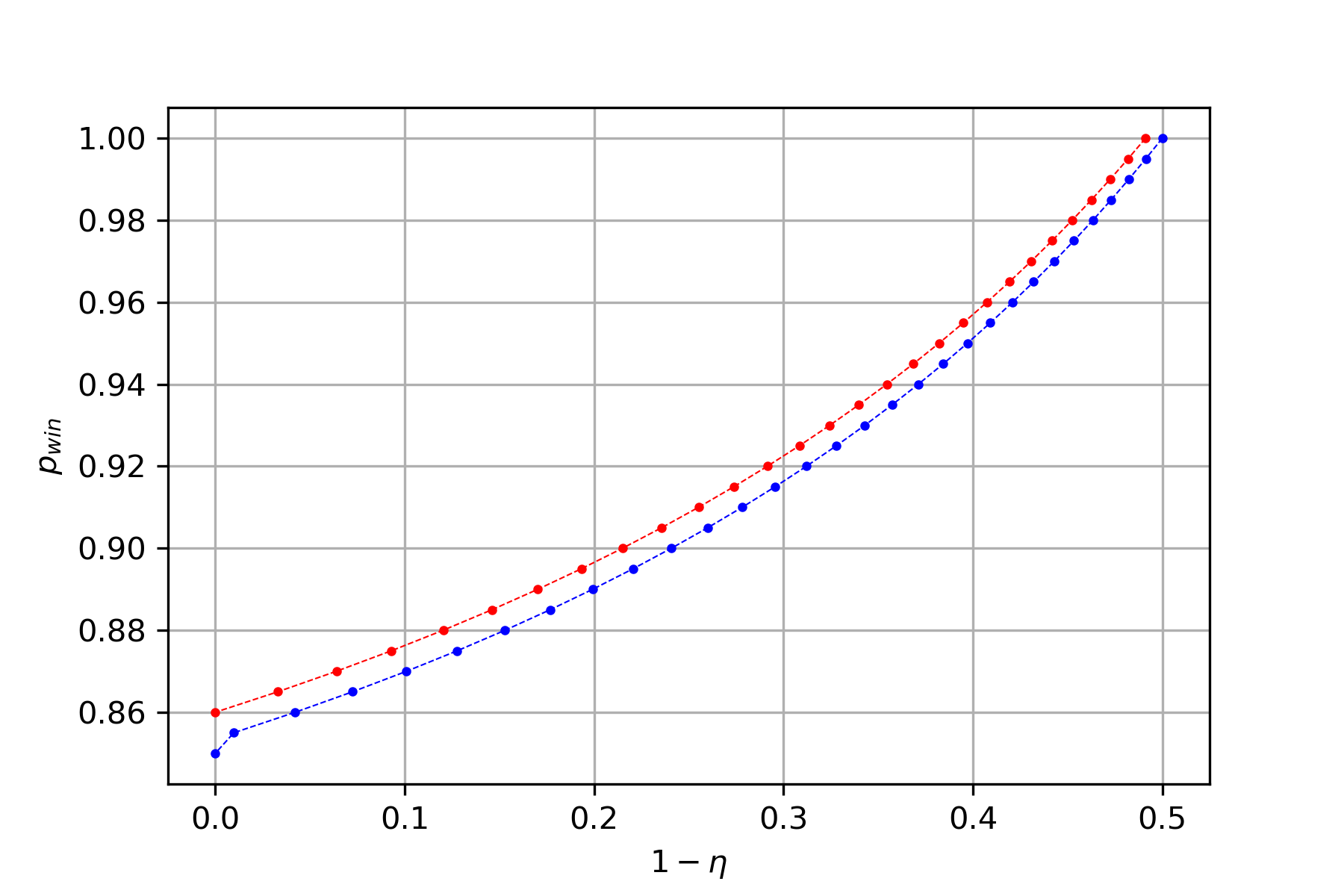
Figure 4: Upper bounds of the winning probability given by (19) (blue dots), (equivalent representation of the blue pluses in Fig. 2), which corresponds to a numerical representation of the function $w(\eta)$. Red dots correspond to a numerical representation of the function $\tilde{w}^{\xi}(\eta)$, which is obtained by adding $\xi=0.005$ to the relaxation of (19) where the attackers are allowed to make errors with probability $\xi$. The continuous interpolation between values is meant for a better viewing of the plot.

Now, we prove that the difference between the probabilities obtained by two quantum states projected into the same space is upper bounded by their trace distance. We then use this result to show that if two quantum states can be used to successfully attack around of the protocol with high probability with the POVMs $\{A^{xy}_{a}\}\textrm{ and }\{B^{xy}_{b}\}$ for input $0$ and $1$ of a $q-$qubit strategy for $\mathrm{QPV}_{\mathrm{BB84}}^{\eta,f}$, respectively, these two states have to differ by at least a certain amount. These results are formalized in the next proposition and lemma.

Proposition 3.5.

Let $\left|\psi\right\rangle$ and $\left|\varphi\right\rangle$ be two quantum states of (the same) arbitrary dimension, and let $\mathcal{D}(\left|\psi\right\rangle,\left|\varphi\right\rangle)$ denote their trace distance. Then, for every projector $\Pi$,

$$\lvert\mathrm{Tr}\left[(\left|\psi\rangle\langle\psi\right|-\left|\varphi\rangle\langle\varphi\right|)\Pi\right]\rvert\leq\mathcal{D}(\left|\psi\right\rangle,\left|\varphi\right\rangle).$$ (30)

Proof.

There exist $Q$ and $S$ positive operators with orthogonal support [NC11, Chapter 9] such that

$$\left|\psi\rangle\langle\psi\right|-\left|\varphi\rangle\langle\varphi\right|=Q-S,\textrm{ and }\mathcal{D}(\left|\psi\right\rangle,\left|\varphi\right\rangle)=\mathrm{Tr}\left[Q\right]=\mathrm{Tr}\left[S\right].$$ (31)

Then,

$$\begin{split}\mathrm{Tr}\left[(\left|\psi\rangle\langle\psi\right|-\left|\varphi\rangle\langle\varphi\right|\Pi)\right]&=\mathrm{Tr}\left[(Q-S)\Pi\right]=\mathrm{Tr}\left[Q\Pi\right]-\mathrm{Tr}\left[S\Pi\right]\leq\mathrm{Tr}\left[Q\Pi\right]\\ &\leq\mathrm{Tr}\left[Q\right]\|\Pi\|=\mathcal{D}(\left|\psi\right\rangle,\left|\varphi\right\rangle),\end{split}$$ (32)

where we used that $S$ is positive definite and $\|\Pi\|=1$. ∎

Lemma 3.6.

Let $\left|\psi\right\rangle$ and $\left|\varphi\right\rangle$ be such that $p_{\psi}^{1,\eta}\geq\tilde{w}^{\xi}(\eta)+\Delta$ and $p_{\varphi}^{0,\eta}\geq\tilde{w}^{\xi}(\eta)+\Delta$, for some $\Delta>0$, which, due to Definition 3.4, $\left|\psi\right\rangle\in\mathcal{S}_{0}^{\varepsilon}$ and $\left|\varphi\right\rangle\in\mathcal{S}_{1}^{\varepsilon}$, for $\varepsilon=1-(\tilde{w}^{\xi}(\eta)+\Delta)$. Then,

$$\mathcal{D}(\left|\psi\right\rangle,\left|\varphi\right\rangle)\geq\eta\Delta.$$ (33)

Notice that the hypothesis of Lemma 3.6 imply that $p_{\psi}^{1,\eta},p_{\varphi}^{0,\eta}\geq\tilde{w}^{\xi}(\eta)+\Delta>w(\eta)$ and thus these two states perform better in inputs $1$ and $0$, respectively, than any state would perform on average on both inputs. The greater is $\Delta$, the better they can perform.

Proof.

Let $\xi=\mathcal{D}(\left|\psi\right\rangle,\left|\varphi\right\rangle)$ and $\psi=\left|\psi\rangle\langle\psi\right|$, $\varphi=\left|\varphi\rangle\langle\varphi\right|$. Subtracting and adding $\varphi$ to $\psi$ in Equation (26) for $i=1$,

$$\begin{split}\eta p_{\psi}^{1,\eta}&=\max_{\begin{subarray}{c}\{A_{a}^{1},B_{a}^{1}\}_{a\in\{0,1,\perp\}}\\ \textrm{with }\mathrm{Tr}\left[\psi A_{a}^{1}B_{b}^{1}\right]=0,\forall a\neq b\in\{0,1,\perp\},\\ \textrm{and }\mathrm{Tr}\left[\psi A_{\perp}^{1}B_{\perp}^{1}\right]=1-\eta\end{subarray}}\sum_{a\in\{0,1\}}\mathrm{Tr}\left[(\psi-\varphi+\varphi)V_{a}^{1}A_{a}^{1}B_{a}^{1}\right]\\ &\leq 2\xi+\max_{\begin{subarray}{c}\{A_{a}^{1},B_{a}^{1}\}_{a\in\{0,1,\perp\}}\\ \textrm{with }\mathrm{Tr}\left[\psi A_{a}^{1}B_{b}^{1}\right]=0,\forall a\neq b\in\{0,1,\perp\},\\ \textrm{and }\mathrm{Tr}\left[\psi A_{\perp}^{1}B_{\perp}^{1}\right]=1-\eta\end{subarray}}\sum_{a\in\{0,1\}}\mathrm{Tr}\left[\varphi V_{a}^{1}A_{a}^{1}B_{a}^{1}\right]\\ &\leq 2\xi+\max_{\begin{subarray}{c}\{A_{a}^{1},B_{a}^{1}\}_{a\in\{0,1,\perp\}}\\ \textrm{with }\mathrm{Tr}\left[\varphi A_{a}^{1}B_{b}^{1}\right]\leq\xi,\forall a\neq b\in\{0,1,\perp\},\\ \textrm{and }(1-\eta)-\xi\leq\mathrm{Tr}\left[\varphi A_{\perp}^{1}B_{\perp}^{1}\right]\leq(1-\eta)+\xi\end{subarray}}\sum_{a\in\{0,1\}}\mathrm{Tr}\left[\varphi V_{a}^{1}A_{a}^{1}B_{a}^{1}\right]=2\xi+\eta\tilde{p}_{\varphi}^{1,\eta,\xi},\end{split}$$ (34)

where the first bound by $2\xi$ comes from (30) and we used that, because of (30), the condition $\mathrm{Tr}\left[\psi A_{a}^{1}B_{b}^{1}\right]=0,\forall a\neq b\in\{0,1,\perp\}$ implies $\mathrm{Tr}\left[\varphi A_{a}^{1}B_{b}^{1}\right]\leq\xi,\forall a\neq b\in\{0,1,\perp\}$ and condition $\mathrm{Tr}\left[\psi A_{\perp}^{1}B_{\perp}^{1}\right]=1-\eta$ implies $(1-\eta)-\xi\leq\mathrm{Tr}\left[\varphi A_{\perp}^{1}B_{\perp}^{1}\right]\leq(1-\eta)+\xi$.
Combining (34), the hypothesis $p_{\psi}^{1,\eta}\geq\tilde{w}^{\xi}(\eta)+\Delta$ and Equation (29), we have

$$\tilde{p}_{\varphi}^{0,\eta,\xi}\leq\tilde{w}^{\xi}(\eta)-\Delta+\frac{2\xi}{\eta}.$$ (35)

On the other hand, since $\tilde{p}_{\varphi}^{0,\eta,\xi}$ is obtained by relaxing the restrictions of $p_{\varphi}^{0,\eta}$, we have that $\tilde{p}_{\varphi}^{0,\eta,\xi}\geq p_{\varphi}^{0,\eta}$ and, by hypothesis, $p_{\varphi}^{0,\eta}\geq\tilde{w}^{\xi}(\eta)+\Delta$. These, together with (35), lead to $\xi\geq\eta\Delta$. ∎

Notice that Lemma 3.6 implies that Alice and Bob in some sense have to decide what strategy they follow before they communicate. Consequently, if the dimension of the state they share is small enough, a classical description of the first part of their strategy yields a compression of $f$. The notion of the following definition captures this classical compression.

Definition 3.7.

[BCS22] Let $q$, $k$, $n\in\mathbb{N}$, $\varepsilon>0$. Then,

$$g:\{0,1\}^{3k}\to\{0,1\}$$

is an $(\varepsilon,q)$-classical rounding of size $k$ if for all $f:\{0,1\}^{2n}\to\{0,1\}$, for all states $\left|\psi\right\rangle$ on $2q+1$ qubits, for all $l\in\{1,\ldots,2^{2n}\}$ and for all $(\varepsilon,l)$-perfect $q$-qubit strategies for $\mathrm{QPV}_{\mathrm{BB84}}^{f}$, there are functions $f_{A}:\{0,1\}^{n}\to\{0,1\}^{k}$, $f_{B}:\{0,1\}^{n}\to\{0,1\}^{k}$ and $\lambda\in\{0,1\}^{k}$ such that $g(f_{A}(x),f_{B}(y),\lambda)=f(x,y)$ on at least $l$ pairs $(x,y)$.

Lemma 3.8.

[LT91] Let $|||*|||$ be any norm on $\mathbb{R}^{n_{0}}$, for $n_{0}\in\mathbb{N}$. There is a $\delta$-net $S$ of the unit sphere of $(\mathbb{R}^{n_{0}},|||*|||)$ of cardinality at most $(1+2/\delta)^{n_{0}}$.

Lemma 3.9.

Let $\Delta>0$, and let $0\leq\varepsilon\leq\varepsilon_{0}$, where $\varepsilon_{0}$ is such that $\left|\psi_{i}\right\rangle\in\mathcal{S}_{i}^{\varepsilon}$ for $i\in\{0,1\}$ implies $\mathcal{D}(\left|\psi_{0}\right\rangle,\left|\psi_{1}\right\rangle)\geq\eta\Delta$. Then there is an $(\varepsilon,q)$-classical rounding of size $k=\log(\lceil\frac{4}{2^{\frac{2}{3}}(\eta\Delta+2)^{\frac{1}{3}}-2}\rceil)2^{2q+2}$.

Proof.

Sketch (see Lemma 5.4 for a detailed proof of the generalized version). Consider a $\delta$-net in Euclidean norm for the set of pure state on $2q+1$ qubits, where the net has cardinality at most $2^{k}$. Following the proof of Lemma 5.4 analogously, we have that $\delta$ is such that $3\delta+3\delta^{2}+\delta^{3}<\eta\Delta/2,$ which holds for $\delta<(2+\eta\Delta)^{\frac{1}{3}}/2^{\frac{1}{3}}-1$. By Lemma 3.8, we obtain the size $k=\log(\lceil\frac{4}{2^{\frac{2}{3}}(\eta\Delta+2)^{\frac{1}{3}}-2}\rceil)2^{2q+2}$. The remaining part of the proof is analogous to the proof of Lemma 5.4. ∎

Lemma 3.10.

Let $\Delta=0.013$, $\eta\in(0.509,1]$, $\varepsilon\in[0,1]$ $n$, $k$, $q\in\mathbb{N}$, $n\geq 10$. Moreover, fix an $(\varepsilon,q)$-classical rounding $g$ of size $k$ with $k=\log(\lceil\frac{4}{2^{\frac{2}{3}}(\eta\Delta+2)^{\frac{1}{3}}-2}\rceil)2^{2q+2}$. Let $q\leq\frac{1}{2}n-5$. Then, a uniformly random $f:\{0,1\}^{2n}\to\{0,1\}$ fulfills the following with probability at least $1-2^{-2^{n}}$: For any $f_{A}:\{0,1\}^{n}\to\{0,1\}^{k}$, $f_{B}:\{0,1\}^{n}\to\{0,1\}^{k}$, $\lambda\in\{0,1\}^{k}$, the equality $g(f_{A}(x),f_{B}(y),\lambda)=f(x,y)$ holds on less than $3/4$ of all pairs $(x,y)$.

Proof.

Sketch (see below Lemma 3.10 for a detailed proof of the generalized version). We want to estimate the probability that for a randomly chosen $f$, we can find $f_{A}$ and $f_{B}$ such that the corresponding function $g$ is such that $\mathbb{P}_{x,y}[f(x,y)=g(f_{A}(x),f_{B}(y),\lambda)]\geq 3/4$. In a similar manner as in (58), we have that

$$\mathbb{P}[f:\exists f_{A},f_{B},\lambda\textrm{ s.t. }\mathbb{P}_{x,y}[f(x,y)=g(f_{A}(x),f_{B}(y),\lambda)]]\leq 2^{(2^{n+1}+1)k}2^{2^{2n}h(1/4)}2^{-2^{2n}},$$ (36)

where $h$ denotes the binary entropy function. If $q\leq n/2-5$ and $k=\log(\lceil\frac{4}{2^{\frac{2}{3}}(\eta\Delta+2)^{\frac{1}{3}}-2}\rceil)2^{2q+2}$, with $\Delta=0.013$, for $\eta\in(0.509,1]$, the above expression is strictly upper bounded by $2^{-2^{n}}$. ∎

Lemma 3.10 shows that if the dimension of the initial state that Alice and Bob hold is small enough, any $(\varepsilon,3/4\cdot 2^{2n})$-perfect $q$-qubit strategy needs a number of qubits which is linear in $n$. This leads to our first main theorem:

Lemma 3.11.

Consider the most general attack to a round of the $\mathrm{QPV}_{\mathrm{BB84}}^{\eta,f}$ protocol for a transmission rate ${\eta\in(0.509,1]}$. Let $\Delta=0.013$. If the attackers respond with probability $\eta$ and control at most $q$ qubits at the beginning of the protocol, and $q$ is such that

$$q\leq\frac{n}{2}-5,$$ (37)

then

$$\mathbb{P}[\textsc{V}_{\textsc{AB}}\neq\textsc{ Correct}\mid\textsc{V}_{\textsc{AB}}\neq\textsc{No photon}]\geq\frac{1}{4}[1-(\tilde{w}^{\xi}(\eta)+\Delta)].$$ (38)

The proof of Lemma 3.11 is a particular case of the proof of Theorem 5.6. See Fig. 5 for a representation of the bound (38). As stated below, if $p_{err}$ is below these bounds, the attackers’ probability of being correct if they play is strictly smaller than the corresponding prover’s probability.

Theorem 3.12.

If the attackers respond with probability $\eta$ and control at most $q\leq\frac{n}{2}-5$ qubits at the beginning of the $\mathrm{QPV}_{\mathrm{BB84}}^{\eta,f}$ protocol and the honest prover’s error is such that $p_{err}<\frac{1}{4}[1-(\tilde{w}^{\xi}(\eta)+\Delta)]$, where $\Delta=0.013$, then the probability that the attackers are correct given that they respond is strictly smaller than the corresponding prover’s probability, i.e.

$$\mathbb{P}[\textsc{V}_{\textsc{AB}}=\textsc{ Correct}\mid\textsc{V}_{\textsc{AB}}\neq\textsc{No photon}]<\mathbb{P}[\textsc{V}_{\textsc{P}}=\textsc{ Correct}\mid\textsc{V}_{\textsc{P}}\neq\textsc{No photon}]=1-p_{err}.$$ (39)

Theorem 3.12 is an immediate consequence of Lemma 3.11. We see then that if $p_{err}<\frac{1}{4}[1-(\tilde{w}^{\xi}(\eta)+\Delta)]$ the $\mathrm{QPV}_{\mathrm{BB84}}^{\eta,f}$ protocol is secure even in the presence of photon loss and attackers who pre-share entanglement.

Figure 5: Lower bounds (red triangles pointing up) given by Theorem 3.11 on the probabilities that the attackers are not correct given that they answer.

4 The $\mathrm{QPV}_{m_{\theta\varphi}}^{\eta}$ protocol

In Section 2 we showed security of $\mathrm{QPV}_{\mathrm{BB84}}^{\eta}$  protocol for unentangled attackers. Nevertheless, the protocol was shown to be secure only for transmission rate $\eta>\frac{1}{2}$, which is still very hard for current technology to achieve. For this reason, we propose a protocol which generalizes $\mathrm{QPV}_{\mathrm{BB84}}^{\eta}$  to more basis settings, for which we can apply similar techniques to prove security in the lossy case. In this section, we generalize the results of Section 3, showing security for non-entangled attackers and reaching arbitrary big photon loss.

Independently and around the same time, Buhrman, Schaffner, Speelman, Zbinden [Spe16b, Chapter 5] and Qi and Siopsis [QS15] introduced extensions of the $\mathrm{QPV_{BB84}}$ protocol. Both are based on allowing the verifiers to choose among more than two different qubit bases, which for the $\mathrm{QPV}_{\mathrm{BB84}}$  protocol corresponded to the computational and the Hadamard basis. The protocol in [Spe16b] allows $V_{0}$ choosing among $m$, for an arbitrary $m\geq 2$, different orthonormal bases in the meridian $\varphi=0$ of the Bloch sphere depending on the angle $\theta\in[0,\pi)$, where these are uniformly distributed, i.e. $\theta\in\{\frac{0}{m}\pi,...,\frac{m-1}{m}\pi\}$, and the bases are $\{\left|0_{\theta}\right\rangle,\left|1_{\theta}\right\rangle\}$, where

$$\begin{split}&\left|0_{\theta}\right\rangle:=\cos\frac{\theta}{2}\left|0\right\rangle+\sin\frac{\theta}{2}\left|1\right\rangle,\hskip 28.45274pt\left|1_{\theta}\right\rangle:=\sin\frac{\theta}{2}\left|0\right\rangle-\cos\frac{\theta}{2}\left|1\right\rangle.\end{split}$$ (40)

Recall that the $\mathrm{QPV_{BB84}}$ protocol is recovered taking $m=2$, where $\theta=0$ and $\theta=\frac{\pi}{2}$ correspond to the computational and Hadamard basis, respectively. On the other hand, the extension in [QS15] allows the verifiers to choose among $m$ encoding bases over the whole Bloch sphere, however such an extension only works for $m$ large enough and not all large integers are allowed.

Here we present a similar extension allowing to choose $m$ random bases over the Bloch sphere for all $m\geq 2$, which works regardless whether $m$ is large or small, and we prove that this translates to better security in case terms of the loss-tolerance of the quantum information in an experimental implementation. We add the $\varphi$ parameter corresponding to the azimuth angle to the states in (40) as a phase $e^{i\varphi}$ in front of $\left|1\right\rangle$, in a similar way as in [QS15]. We do however use a slightly different procedure than [QS15] to compute the precise angles, to make the basis choice more uniform (see below).

4.1 Discrete uniform choice of basis over the Bloch sphere

In order to avoid accumulation of points in the sphere around the poles due to the unit sphere area element $d\Omega=\sin\theta d\theta d\varphi$, a continuous uniform distribution of points can be made by taking [Wei]

$$\begin{split}&\theta=\cos^{-1}(2u-1),\hskip 28.45274pt\varphi=2\pi v,\end{split}$$ (41)

where $u$ and $v$ are uniformly distributed over the interval $(0,1)$. Notice that allowing $\varphi\in[0,2\pi)$ would imply to have duplicate bases (i.e., the same basis vectors in different order), thus, $\varphi$ will be restricted to take values in the range $[0,\pi)$. Moreover, in the discrete case we are interested also in the north pole of the sphere ($\theta=0$), corresponding to the computational basis, and therefore in order to include it, discretizing the sphere with $m_{\theta}$ different $\theta$ and with $m_{\varphi}$ different $\varphi$, the 0 must be included in the range of $u$, i.e.  $u\in\{\frac{0}{m_{\theta}},...,\frac{m_{\theta}-1}{m_{\theta}}\}$. Similarly, in order to have the Hadamard basis (and the bases in between them in the meridian $\varphi=0$), $v\in\{\frac{0}{m_{\varphi}},...,\frac{m_{\varphi}-1}{m_{\varphi}}\}$. Let $\tilde{u}:=m_{\theta}u$ and $\tilde{v}:=m_{\varphi}v$, which determine the $m_{\theta}m_{\varphi}$ points of the discretization. Let $x:=\tilde{u}\tilde{v}\equiv m_{\varphi}\tilde{u}+\tilde{v}$, therefore, given $x\in[m_{\theta}m_{\varphi}]$, one can recover $\tilde{u}=\left\lfloor x/m_{\varphi}\right\rfloor$ and $\tilde{v}=x\bmod m_{\varphi}$, where $\left\lfloor*\right\rfloor$ stands for the floor function. Notice that this discrete parametrization has $m_{\varphi}$ degenerate points for $\tilde{u}=m_{\theta}-1$, corresponding to $(\theta=0,\varphi)$, which can be easily removed by $x$ taking values in the range $\{0,...,m-1\}=:[m]$, where $m:=m_{\varphi}(m_{\theta}-1)+1$. Therefore, we can discretize the bases in the Bloch sphere depending on $x$ so that $\forall x\in[m]$,

$$\begin{split}\theta(x)=\arccos{(\frac{2}{m_{\theta}}(\left\lfloor\frac{x}{m_{\varphi}}\right\rfloor+1)-1)},\hskip 28.45274pt\varphi(x)=\pi\frac{x\bmod m_{\varphi}}{m_{\varphi}}.\end{split}$$ (42)

Then the protocol is extended allowing the verifiers to choose among the bases $\{\left|0_{x}\right\rangle,\left|1_{x}\right\rangle\}$ for $x\in[m]$, where

$$\begin{split}&\left|0_{x}\right\rangle:=\cos\frac{\theta(x)}{2}\left|0\right\rangle+e^{i\varphi(x)}\sin\frac{\theta(x)}{2}\left|1\right\rangle,\hskip 28.45274pt\left|1_{x}\right\rangle:=\sin\frac{\theta(x)}{2}\left|0\right\rangle-e^{i\varphi(x)}\cos\frac{\theta(x)}{2}\left|1\right\rangle.\end{split}$$ (43)

Note that for any $m$, we can discretize the bases in as many ways as divisors $m-1$ has in the following way: one chooses the number of $\theta$ and $\varphi$ as $(m_{\theta},m_{\varphi})=(d_{m}+1,\frac{m-1}{d_{m}})$, for each $d_{m}$ divisor of $m-1$. See Fig. 6 for the representation of the $\left|0_{x}\right\rangle$ for all $x\in[m]$ in the Bloch sphere for different choices of $m_{\theta}$ and $m_{\varphi}$. The $\left|1_{x}\right\rangle$ corresponds to the diametrically opposite point, and therefore representing the kets $\left|0_{x}\right\rangle$ determines the $m$ orthonormal bases, e.g. the computational basis is associated with the north pole. As examples, the choice $(m,m_{\theta},m_{\varphi})=(2,2,1)$ corresponds to the computational and Hadamard bases, and the choice $(m,m_{\theta},m_{\varphi})=(3,2,2)$ to the computational, Hadamard bases and the basis formed by the eigenvectors of the Pauli $Y$ matrix.

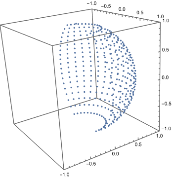
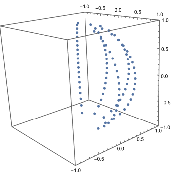
Figure 6: Discretization of $m$ bases in the Bloch sphere, where the points on the surface of the sphere represent the ket $\left|0_{x}\right\rangle$ of the orthonormal basis $\{\left|0_{x}\right\rangle,\left|1_{x}\right\rangle\}$ for $x\in[m]$. (a) $m_{\theta}=m_{\varphi}=20$, (b) $m_{\theta}=10,m_{\varphi}=5$.

Based on Section 4.1, we introduce an extension of the $\mathrm{QPV}_{\mathrm{BB84}}^{\eta}$  protocol, which we denote by $\mathrm{QPV}_{m_{\theta\varphi}}^{\eta}$, where $m_{\theta\varphi}$ is the sort notation of $(m,m_{\theta},m_{\varphi})$.

Definition 4.1.

We define one round of the $\mathrm{QPV}_{m_{\theta\varphi}}^{\eta}$ protocol as:

1. $V_{0}$ and $V_{1}$ secretly agree on $m_{\theta}$, $m_{\varphi}$ and $x\in[m]$. In addition, $V_{0}$ prepares the EPR pair $\left|\Omega\right\rangle=(\left|00\right\rangle+\left|11\right\rangle)/\sqrt{2}$.

2. $V_{0}$ sends one qubit $Q$ of $\left|\Omega\right\rangle$ to $P$ and $V_{1}$ sends $x$ to $P$ coordinating their times so that $Q$ and $x$ arrive at $P$ at the same time.

3. $P$ measures $Q$ in the basis $\{\left|0_{x}\right\rangle,\left|1_{x}\right\rangle\}$ and broadcasts her outcome to $V_{0}$ and $V_{1}$. If, due to experimental losses, $Q$ does not arrive at $P$, she broadcasts ‘no detection’ with the symbol $\perp$.

4. If $V_{0}$ and $V_{1}$ receive both the same bit at the corresponding time, they accept. If they receive $\perp$, they record ‘no photon’.

At the end of the protocol, when sequentially run $r$ times, the verifiers check that the relative frequency of $\perp$ is upper bounded by $1-\eta$. Notice that $\mathrm{QPV}_{\mathrm{BB84}}^{\eta}$ is recovered for $m=2$, with the unique choice of $m_{\theta}=2$ and $m_{\varphi}=1$.

4.2 Security of the $\mathrm{QPV}_{m_{\theta\varphi}}^{\eta}$ protocol under photon loss and non-entangled attackers

In an analogy to the $\mathrm{QPV}_{\mathrm{BB84}}^{\eta}$ protocol, an attack on the $\mathrm{QPV}_{m_{\theta\varphi}}^{\eta}$ protocol can be associated with a MoE (monogamy-of-entanglement) game in the following way. Let $V$ be the register of the qubit of the verifier, with associated Hilbert space $\mathcal{H}_{V}=\mathbb{C}^{2}$, with $\mathcal{X}=[m]$ and $\mathcal{V}=\{0,1\}$. The verifiers perform the collection of measurements

$$\{V_{0}^{x},V_{1}^{x}\}_{x\in[m]},$$ (44)

where $V_{0}^{x}=\left|0_{x}\rangle\langle 0_{x}\right|$ and $V_{1}^{x}=\left|1_{x}\rangle\langle 1_{x}\right|$. The two collaborating parties in the MoE game correspond to the attackers who want to break the protocol with their guess. Then, the attackers Alice and Bob, with associated Hilbert spaces $\mathcal{H}_{A}$ and $\mathcal{H}_{B}$, respectively, have to win against the verifiers $V$ both giving the same outcome to $V$ or declare photon loss. Thus, having a strategy to attack the protocol implies having an strategy for a MoE game. An extension of a strategy for a lossy MoE game, see Section 2, naturally generalizes as $\mathbf{S}^{\eta}_{MoE}=\{\left|\psi\right\rangle,A_{a}^{x},B_{a}^{x}\}_{a\in\{0,1,\perp\},x\in[m]}$.

In [TFKW13] the following upper bound to win a general MoE game is given:

$$p_{win}\leq\frac{1}{|\mathcal{X}|}+\frac{|\mathcal{X}|-1}{|\mathcal{X}|}\sqrt{\max_{x\neq x^{\prime}\in\mathcal{X}}\max_{a,a^{\prime}\in\mathcal{A}}\|\sqrt{V_{a}^{x}}\sqrt{V_{a^{\prime}}^{x^{\prime}}}\|^{2}}.$$ (45)

The security analysis of the $\mathrm{QPV}_{m_{\theta\varphi}}^{\eta}$ protocol will be based, in the same way as the $\mathrm{QPV}_{\mathrm{BB84}}^{\eta}$
protocol, on maximizing the probability that the attackers ‘play’ without being caught:

$$p_{ans}=\frac{1}{m}\sum_{x\in[m],a\in\{0,1\}}\left\langle\psi\right|A_{a}^{x}B_{a}^{x}\left|\psi\right\rangle.$$ (46)

As in the $\mathrm{QPV}_{\mathrm{BB84}}^{\eta}$  protocol, the constraints will be the linear constraints implied by $\mathbf{S}^{\eta}_{MoE}\in\mathcal{Q}_{\ell}$, the analogous to (17), i.e.,

$$\langle A_{a}^{x}B_{b}^{x}\rangle=0\hskip 14.22636pt\forall a\neq b\in\{0,1,\perp\},\forall x\in[m],$$ (47)

and the inequalities given in Proposition 4.2 bounded by $p_{err}$.

Proposition 4.2.

Let $a,b\in\{0,1\}$, $\alpha_{i}^{a}=\left\langle i_{x^{\prime}}\lvert a_{x}\right\rangle$ and $\beta_{i}^{b}=\left\langle i_{x}\lvert b_{x^{\prime}}\right\rangle$ for $i\in\{0,1\}$. The terms $\langle A_{a}^{x}B_{b}^{x^{\prime}}\rangle$ can be bounded by $p_{err}$ by the two inequalities below:

$$\sum_{ab}(2-\|V_{a}^{x}+V_{b}^{x^{\prime}}\|)\langle A_{a}^{x}B_{b}^{x^{\prime}}\rangle\leq p_{err}\sum_{a}(\langle A_{a}^{x}B_{a}^{x}\rangle+\langle A_{a}^{x^{\prime}}B_{a}^{x^{\prime}}\rangle),$$ (48)

$$\begin{split}&\sum_{a,b}\big{(}4-\|(1+\lvert\beta_{a}^{b}\rvert^{2})V_{a}^{x}+(1+\lvert\alpha_{b}^{a}\rvert^{2})V_{b}^{x^{\prime}}+\beta_{0}^{b}\beta_{1}^{b*}\left|0_{x}\rangle\langle 1_{x}\right|+\beta_{0}^{b*}\beta_{1}^{b}\left|1_{x}\rangle\langle 0_{x}\right|+\alpha_{0}^{a}\alpha_{1}^{a*}\left|0_{x^{\prime}}\rangle\langle 1_{x^{\prime}}\right|\\ &+\alpha_{0}^{a*}\alpha_{1}^{a}\left|1_{x^{\prime}}\rangle\langle 0_{x^{\prime}}\right|\|\big{)}\langle A_{a}^{x}B_{b}^{x^{\prime}}\rangle\leq p_{err}\big{(}(2+\max_{i,j}\lvert\beta_{i}^{j}\rvert^{2})\sum_{a}\langle A_{a}^{x}B_{a}^{x}\rangle+(2+\max_{i,j}\lvert\alpha_{i}^{j}\rvert^{2})\sum_{a}\langle A_{a}^{x^{\prime}}B_{a}^{x^{\prime}}\rangle\big{)},\end{split}$$ (49)

The proof of Proposition 4.2, see Appendix B, relies on combining both expressions in (16),using $A_{0}^{x}+A_{1}^{x}\preceq\mathbb{I}$ and $B_{0}^{x^{\prime}}+B_{1}^{x^{\prime}}\preceq\mathbb{I}$ and bounding terms by the norm of the sums of the projectors $V_{a}^{x}$.

Therefore, using the above constraints, $p_{ans}$ can be upper bounded by the SDP problem:

$$\boxed{\begin{split}&\max\frac{1}{m}\sum_{x}(\langle A_{0}^{x}B_{0}^{x}\rangle+\langle A_{1}^{x}B_{1}^{x}\rangle);\\ &\textrm{subject to: the linear constraints for }\mathbf{S}^{\eta}_{MoE}\in\mathcal{Q}_{\ell},\\ &\textrm{ \hskip 42.67912pt and equations \eqref{eq restriction error epsilon}, \eqref{eq perr constraint sum ab} and \eqref{eq constraint perr 2 simplified}}.\end{split}}$$ (50)

Fig. 7 shows a $SSR$ for the $\mathrm{QPV^{\eta}_{(3,2,2)}}$ protocol obtained from the solutions of the SDP (50) using the Ncpol2sdpa package [Wit15] in Python, see [EFS] for the code. Notice that Fig. 7 shows that the security region for this protocol is greater than the $SR$ of $\mathrm{QPV}_{\mathrm{BB84}}^{\eta}$, meaning that it is more secure. However, analytical bounds on the best attack (even no loss) for these MoE games are so far only known for the BB84 game, and therefore we can not show tightness of our results beyond the $\mathrm{QPV}_{\mathrm{BB84}}^{\eta}$  protocol – a gap between our best upper bounds and lower bounds remains. Numerical results from (50) show that for different arbitrary $m$, $p_{ans}$ for $p_{err}=0$ is upper bounded by $\frac{1}{m}$, which is attainable by the strategy of Alice randomly guessing $x$, measuring in this basis, broadcasting the outcome and answering if she was correct and otherwise claiming no photon.

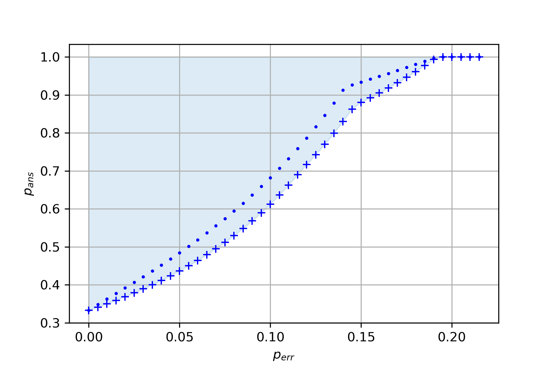
Figure 7: Solutions of the first (blue dots) and second level (blue pluses) of the NPA hierarchy for the SDP (50) highlighting a $SSR\subseteq SR$ of the $\mathrm{QPV^{\eta}_{(3,2,2)}}$ protocol in light blue.

As stated above, finding the smallest $p_{err}$ such that $p_{ans}=1$ can be used to upper bound the winning probability $p_{win}$. Fig. 8 shows the values upper bounding $p_{win}$ with the SDP (50), showing security of the protocol for different $(m,m_{\theta},m_{\varphi})$, compared with the upper bound obtained by (45) [TFKW13], when the attackers always ‘play’, where significant differences between both methods can be appreciated.

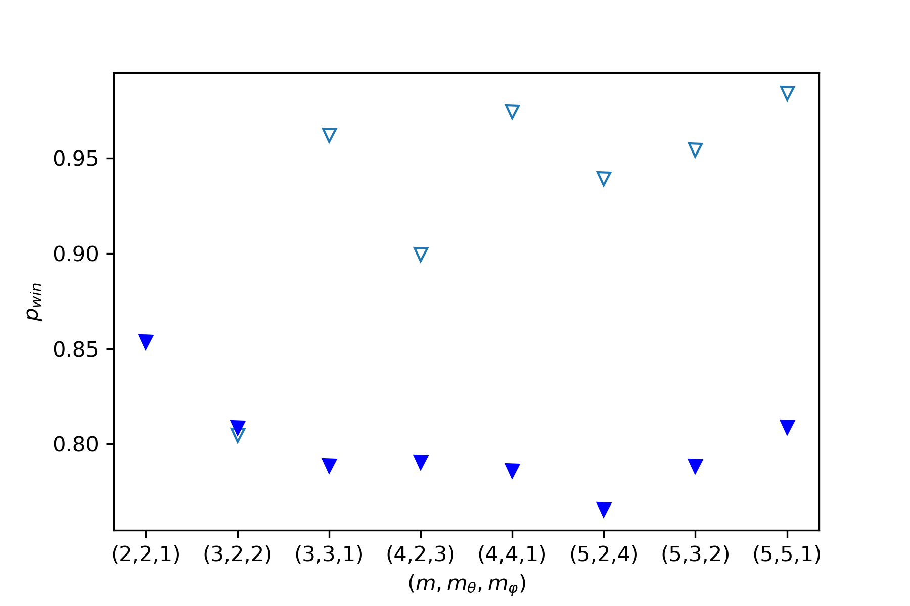
Figure 8: Upper bounds of $p_{win}$ using (45) (empty triangles) and the solution of SDP (50) (solid triangles) for the $\mathrm{QPV}_{m_{\theta\varphi}}^{\eta}$ protocol for different values of $(m,m_{\theta},m_{\varphi})$.

5 The $\mathrm{QPV}^{\eta,f}_{m_{\theta\varphi}}$ protocol and its security under entangled attackers

In Section 3 we have shown that $\mathrm{QPV}_{\mathrm{BB84}}^{\eta,f}$ is secure against entangled attackers if they hold a bounded number of qubits, but it is currently non-implementable experimentally due to the fact that it is not secure for $\eta\leq 1/2$. On the other hand, in Section 4 we have shown that extending the $\mathrm{QPV}_{\mathrm{BB84}}^{\eta}$  protocol to $m$ bases allows for more resistance to photon loss. In this section, we use the results from Section 4 to prove Lemma 5.1. This lemma will form the key tool to re-apply the analysis in [BCS22] to our case, and as a consequence we will show that the $\mathrm{QPV}^{\eta,f}_{m_{\theta\varphi}}$ protocol is secure against entangled attackers (and more loss-tolerant than $\mathrm{QPV}_{\mathrm{BB84}}^{\eta,f}$). The results in this section are proven for arbitrary $m$, however they are based on solving the SDP described in (50), which needs $m$ to be fixed. Here, we obtain numerical results for the two particular cases $m_{\theta\varphi}=(3,2,2)$ and $m_{\theta\varphi}=(5,3,2)$, but to obtain the results for any $m_{\theta\varphi}$ that would potentially be applied experimentally, one just needs to solve (50) and the corresponding relaxation, see below. Moreover, here we solve the semidefinite programs for a complete range of $p_{err}$, thereby obtaining an exhaustive characterization for the fixed $m_{\theta\varphi}$, but for an experimental implementation it would just be needed to solve the SDPs for the ranges that the experimental set-up requires.

For some $n\in\mathbb{N}$, consider a $2n$-bit function $f:\{0,1\}^{n}\times\{0,1\}^{n}\to[m]$. One round of the $m_{\theta\varphi}$-basis lossy-function protocol, denoted by $\mathrm{QPV}^{\eta,f}_{m_{\theta\varphi}}$, is described as in Definition 3.1 changing the range of $f$. The corresponding general attack is described as in Attack 3.2, extended by changing the range of the function $f$, and similarly for the $q$-qubit strategy.

With the same reasoning as in Section 3, from (50) and its corresponding relaxation given by $\langle A^{x}_{a}B^{x}_{b}\rangle\leq\xi$, for all $a\neq b$, we have that there exists functions $w_{m_{\theta\varphi}}(\eta)$ and $\tilde{w}_{m_{\theta\varphi}}^{\xi}(\eta)$ such that

$$\frac{1}{m}\sum_{i\in[m]}p_{\phi}^{i,\eta}\leq w_{m_{\theta\varphi}}(\eta),$$ (51)

and

$$\frac{1}{m}\sum_{i\in[m]}\tilde{p}_{\phi}^{i,\eta,\xi}\leq\tilde{w}^{\xi}_{m_{\theta\varphi}}(\eta),$$ (52)

that are such that $w_{m_{\theta\varphi}}(\eta)\leq\tilde{w}_{m_{\theta\varphi}}^{\xi}(\eta)$. The probabilities $p_{\phi}^{i,\eta}$ and $\tilde{p}_{\phi}^{i,\eta,\xi}$ are as in (26) and (28), respectively, with $i\in[m]$. See Fig. 9 for a numerical approximation of the functions $w_{m_{\theta\varphi}}(\eta)$ and $\tilde{w}_{m_{\theta\varphi}}^{\xi}(\eta)$ for different $m_{\theta\varphi}$, see [EFS] for the code.

Now, we show a lemma that formalizes the idea that if a set of $m$ quantum states can be used to be correct with high probability in an attack of the protocol, then, their average distance is lower bounded by a certain amount. This has the interpretation that these states cannot all be simultaneously arbitrarily close. This means that exists an $\varepsilon_{0}$ such that for all $\varepsilon\leq\varepsilon_{0}$, $\bigcap_{i\in[m]}\mathcal{S}_{i}^{\varepsilon}=\emptyset$, where $\mathcal{S}_{i}^{\varepsilon}$ is defined as in Definition 3.4 with $i\in[m]$.

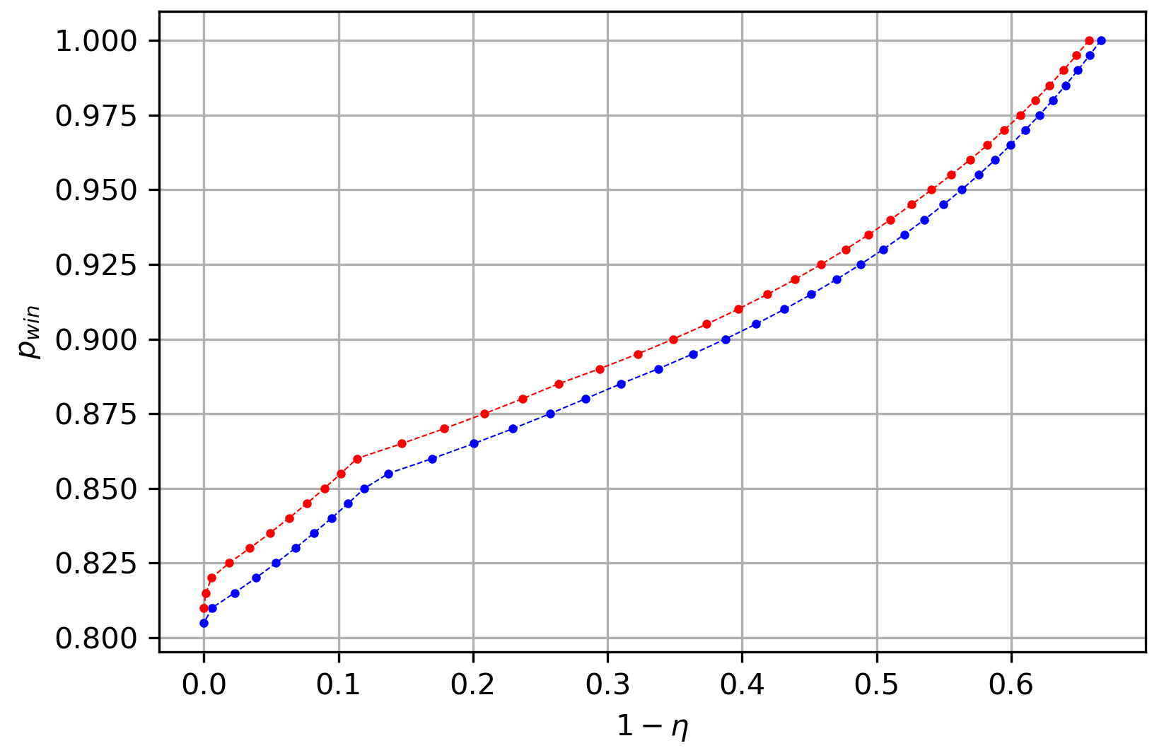
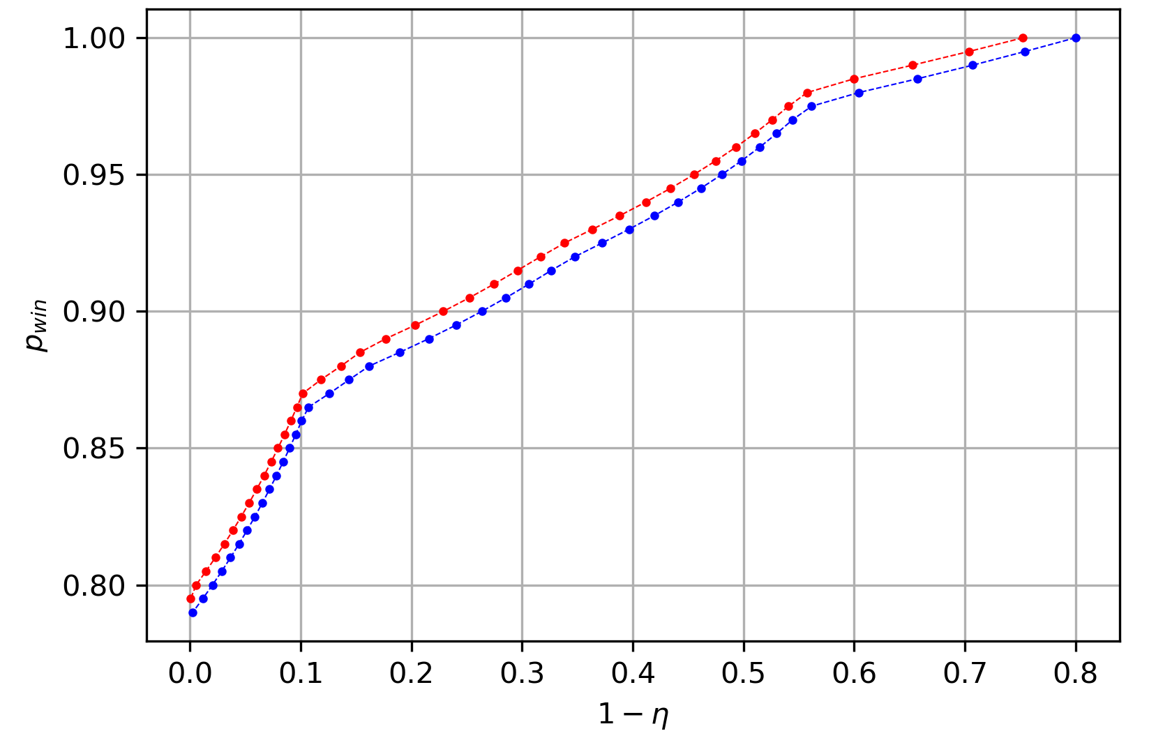
Figure 9: Upper bounds of the winning probability given by (50) (blue dots), corresponding to a numerical representation of the function $w_{m_{\theta\varphi}}(\eta)$. Red dots correspond to a numerical representation of the function $\tilde{w}^{\xi}_{m_{\theta\varphi}}(\eta)$, which is obtained by adding $\xi=0.005$ to the relaxation of (50) where the attackers are allowed to make errors with probability $\xi$, for (a) $m_{\theta\varphi}=(3,2,2)$, and (b) $m_{\theta\varphi}=(5,3,2)$. The values in (a) and (b) are obtained by the level 2 and level ‘1+AB’ of the NPA hierarchy, respectively. The continuous interpolation between values is meant for a better viewing of the plot.

Lemma 5.1.

Let $\left|\psi_{i}\right\rangle$ be such that $p^{i,\eta}_{\psi_{i}}\geq\tilde{w}^{\xi}_{m_{\theta\varphi}}(\eta)+\Delta$, for all $i\in[m]$, for some $\Delta>0$, which implies that  $\left|\psi_{i}\right\rangle\in\mathcal{S}_{i}^{\varepsilon}$, for $\varepsilon=1-(\tilde{w}^{\xi}(\eta)+\Delta)$. Then, for all $j\in[m]$

$$\underset{i\in[m]}{\mathbb{E}}[\mathcal{D}(\left|\psi_{j}\right\rangle,\left|\psi_{i}\right\rangle)]\geq\frac{\eta\Delta}{2}.$$ (53)

Proof.

Let $\xi_{ij}=\mathcal{D}(\left|\psi_{j}\right\rangle,\left|\psi_{i}\right\rangle)$ and let $\xi=\max_{ij}\xi_{ij}$. From an analogous application of equation (34), we have that for all $i,j\in[m]$,

$$p^{i,\eta}_{\psi_{i}}\leq\frac{2}{\eta}\xi_{ij}+\tilde{p}^{i,\eta,\xi_{ij}}_{\psi_{j}}\leq\frac{2}{\eta}\xi_{ij}+\tilde{p}^{i,\eta,\xi}_{\psi_{j}},$$ (54)

where in the second inequality we used that replacing $\xi_{ij}$ by $\xi$ is a relaxation of the restrictions of the maximization (28). Fixing $j$ and summing over $i$,

$$\sum_{i\in[m]}p^{i,\eta}_{\psi_{i}}\leq\frac{2}{\eta}\sum_{i\in[m]}\xi_{ij}+\sum_{i\in[m]}\tilde{p}^{i,\eta,\xi}_{\psi_{j}}.$$ (55)

By hypothesis, each term in the left-hand side is lower bounded by $\tilde{w}^{\xi}_{m_{\theta\varphi}}(\eta)+\Delta$. This, together with (52), lead to (53). ∎

Since Lemma 5.1 implies that if a set of $m$ states ‘performs well’ on their respective inputs, their average distance with respect to an arbitrary state is at least a certain amount, meaning that there are at least two states that differ by such an amount, it has as consequence that Alice and Bob in some sense have to decide (at least one) strategy not to follow before they communicate. Consequently, if the dimension of the state they share is small enough, a classical description of the first part of their strategy yields a compression of $f$. The notion of the following definition captures this classical compression.

Definition 5.2.

Let $q,k,n\in\mathbb{N}$, $\varepsilon>0$. Then,

$$g_{m_{\theta\varphi}}:\{0,1\}^{3k}\rightarrow 2^{[m]}\setminus[m]$$ (56)

is an $(\varepsilon,q)$-classical rounding restriction of size $k$ is for all $f:\{0,1\}^{2n}$, for all states $\left|\phi\right\rangle$ on $2q+1$ qubits, for all $l\in\{1,...,2^{2n}\}$ and for all $(\varepsilon,l)$-perfect $q$-qubit strategies for $QPV^{f}_{m_{\theta\varphi}}$, there are functions $f_{A}:\{0,1\}^{n}\rightarrow\{0,1\}^{k}$, $f_{B}:\{0,1\}^{n}\rightarrow\{0,1\}^{k}$ and $\lambda\in\{0,1\}^{k}$ such that $f(x,y)\in g(f_{A}(x),f_{B}(y),\lambda)$.

Lemma 5.3.

[BCS22] Let $\left|x\right\rangle,\left|y\right\rangle\in\mathbb{C}^{d}$, for $d\in\mathbb{N}$, be two unit vectors. Then, $\mathcal{D}(\left|x\right\rangle,\left|y\right\rangle)\leq\|\left|x\right\rangle-\left|y\right\rangle\|_{2}$.

Lemma 5.4.

Let $\Delta>0$, and let $0\leq\varepsilon\leq\varepsilon_{0}$, where $\varepsilon_{0}$ is such that $\left|\psi_{i}\right\rangle\in\mathcal{S}_{i}^{\varepsilon}$, implies $\underset{i\in[m]}{\mathbb{E}}[\mathcal{D}(\left|\psi_{j}\right\rangle,\left|\psi_{i}\right\rangle)]\geq\frac{\eta\Delta}{2}$. Then there exists an $(\varepsilon,q)$-classical rounding restriction of size $k=\log(\lceil\frac{4}{2^{\frac{1}{3}}(\eta\Delta+4)^{\frac{1}{3}}-2}\rceil)2^{2q+2}$.

Proof.

We follow the same techniques as in the proof of Lemma 3.12 in [BCS22]. Let $\delta=\frac{\sqrt[3]{\eta\Delta+4}}{2^{2/3}}-1-\epsilon$, where $\epsilon>0$ is infinitesimally small, and consider $\delta$-nets $\mathcal{N}_{S}$, $\mathcal{N}_{A}$ and $\mathcal{N}_{B}$, where the first is for the set of pure states on $2q+1$ qubits in Euclidean norm and the other nets are for the set of unitaries in dimension $2^{q}$ in operator norm. They are such that $\lvert\mathcal{N}_{S}\rvert$, $\lvert\mathcal{N}_{A}\rvert$, $\lvert\mathcal{N}_{B}\rvert\leq 2^{k}$. Let $\left|\varphi\right\rangle\in\mathcal{N}_{S}$, $U_{A}\in\mathcal{N}_{A}$, and $U_{B}\in\mathcal{N}_{B}$ be the elements with indices $x^{\prime}\in\{0,1\}^{k}$, $y^{\prime}\in\{0,1\}^{k}$ and $\lambda\in\{0,1\}^{k}$, respectively. We define $g$ as $g(x,y,\lambda)=\{j\mid U\otimes V\left|\varphi\right\rangle\in\mathcal{S}_{j}^{\varepsilon}\}$. We are going to show that $g$ is an $(\varepsilon,q)$-classical rounding restriction.
Let $i$, $j$ be such that $\mathcal{D}(\left|\psi_{i}\right\rangle,\left|\psi_{j}\right\rangle)\geq\eta\Delta/2$. Let $\left|\psi\right\rangle$, $\{U_{A}^{x},U_{B}^{y}\}_{xy}$ be from a $q$-qubit strategy for $\mathrm{QPV}^{\eta,f}_{m_{\theta\varphi}}$, and choose $\lambda$, $f_{A}(x)$ and $f_{B}(y)$ to be the closest elements to $\left|\psi\right\rangle$, $U_{A}^{x}$ and $U_{B}^{y}$, respectively, in their corresponding $\delta$-nets in the Euclidean and operator norm, respectively, (if not unique, make an arbitrary choice) and let $\left|\varphi\right\rangle,U_{A},U_{B}$ be their corresponding elements. Assume $U_{A}^{x}\otimes U_{B}^{y}\left|\psi\right\rangle\in\mathcal{S}_{i}^{\varepsilon}$. Then,

$$\begin{split}\mathcal{D}(&U_{A}^{x}\otimes U_{B}^{y}\left|\psi\right\rangle,U_{A}\otimes U_{B}\left|\varphi\right\rangle)\leq\|U_{A}^{x}\otimes U_{B}^{y}\left|\psi\right\rangle-U_{A}\otimes U_{B}\left|\varphi\right\rangle\|_{2}\\ &\leq\|(U_{A}+U_{A}^{x}-U_{A})\otimes(U_{B}+U_{B}^{y}-U_{B})(\left|\varphi\right\rangle+\left|\psi\right\rangle-\left|\varphi\right\rangle)-U_{A}\otimes U_{B}\left|\varphi\right\rangle\|_{2}\\ &\leq 3\delta+3\delta^{2}+\delta^{3}<\frac{\eta\Delta/2}{2},\end{split}$$ (57)

where in the first inequality, we have used Lemma 5.3, in the second, we have used the triangle inequality and the inequality $\|X\otimes Y\left|x\right\rangle\|_{2}\leq\|X\|_{\infty}\|Y\|_{\infty}\|\left|x\right\rangle\|_{2}$, together with $\|U_{A}^{x}-U_{A}\|_{\infty},\\ {\|U_{B}^{y}-U_{B}\|_{\infty}},\|\left|\psi\right\rangle-\left|\varphi\right\rangle\|\leq\delta$, and, finally, in the last inequality we used that $\delta<\frac{\sqrt[3]{\eta\Delta+4}}{2^{2/3}}-1$. Thus, $U_{A}\otimes U_{B}\left|\varphi\right\rangle$ is closer to $\mathcal{S}_{i}^{\varepsilon}$ than to $\mathcal{S}_{j}^{\varepsilon}$.
Consider an $(\varepsilon,l)$-perfect strategy for $\mathrm{QPV}^{\eta,f}_{m_{\theta\varphi}}$  and let $(x,y)$ be such that the attackers are caught with probability at most $\varepsilon$ and such that $f(x,y)=i$. In particular, we have that $U_{A}^{x}\otimes U_{B}^{y}\left|\psi\right\rangle\in\mathcal{S}_{i}^{\varepsilon}$, and because of (57), $f(x,y)\in g(f_{A}(x),f_{B}(y),\lambda)$. Since there are at least $l$ pairs $(x,y)$ fulfilling it, $f(x,y)\in g(f_{A}(x),f_{B}(y),\lambda)$ holds on at least $l$ pairs $(x,y)$ and therefore $g$ is an $(\varepsilon,q)$-classical rounding restriction. The size of $k$ follows from Lemma 3.8.

∎

Given $m_{\theta\varphi}$, we denote by $\eta_{m_{\theta\varphi}}$ the maximum $\eta$ such that $\tilde{w}_{m_{\theta\varphi}}^{\xi}(\eta)+\Delta\leq 1$, e.g. for $m_{\theta\varphi}=(2,2,1)$, i.e. $\mathrm{QPV}_{\mathrm{BB84}}^{\eta}$, that corresponds to 0.509. From (52) and picking $\Delta=0.009$, $\eta_{m_{\theta\varphi}}=0.36$ for $m_{\theta\varphi}=(3,2,2)$ and $\eta_{m_{\theta\varphi}}=0.34$ for $m_{\theta\varphi}=(5,3,2)$ (by picking a smaller $\Delta$, the latter gets closer to 0.2).

Lemma 5.5.

Let $\Delta=0.009$, $\eta\in(\eta_{m_{\theta\varphi}},1]$, $\varepsilon\in[0,1]$ $n$, $k$, $q\in\mathbb{N}$, $n\geq 10$. Moreover, fix an $(\varepsilon,q)$-classical rounding $g$ of size $k$ with $k=\log(\lceil\frac{4}{2^{\frac{1}{3}}(\eta\Delta+4)^{\frac{1}{3}}-2}\rceil)2^{2q+2}$. Let $q\leq\frac{1}{2}n-5$. Then, a uniformly random $f:\{0,1\}^{2n}\to\{0,1\}$ fulfills the following with probability at least $1-2^{-2^{n}}$: For any $f_{A}:\{0,1\}^{n}\to\{0,1\}^{k}$, $f_{B}:\{0,1\}^{n}\to\{0,1\}^{k}$, $\lambda\in\{0,1\}^{k}$, $f(x,y)\in g(f_{A}(x),f_{B}(y),\lambda)$ holds on less than $1-\beta_{m_{\theta\varphi}}$ of all pairs $(x,y)$, for certain $\beta_{m_{\theta\varphi}}>0$ ($\beta_{m_{\theta\varphi}}=0.15$ for $m_{\theta\varphi}=(3,2,2)$ and $\beta_{m_{\theta\varphi}}=0.13$ for $m_{\theta\varphi}=(5,3,2)$ ).

Proof.

For simplicity, denote $\beta_{m_{\theta\varphi}}$ by $\beta$. We want to estimate the probability that for a randomly chosen $f$, we can find $f_{A}$ and $f_{B}$ such that the corresponding function $g$ is such that $\mathbb{P}_{x,y}[f(x,y)\in g_{m_{\theta\varphi}(f_{A}(x),f_{B}(y),\lambda)}]\geq(1-\beta)$.

$$\begin{split}\mathbb{P}&[f:\exists f_{A},f_{B},\lambda\textrm{ s.t. }\mathbb{P}[x,y:f(x,y)\in g_{m_{\theta\varphi}}(f_{A}(x),f_{B}(y),\lambda)]\geq(1-\beta)]\\ &=\frac{\lvert\{f:\exists f_{A},f_{B},\lambda\textrm{s.t. }\mathbb{P}[x,y:f(x,y)\in g_{m_{\theta\varphi}}(f_{A}(x),f_{B}(y),\lambda)]\geq(1-\beta)\}\rvert}{\lvert\{f:\{0,1\}^{2n}\rightarrow[m]\}\rvert}\\ &\leq\frac{\lvert\{f:\exists f_{A},f_{B},\lambda\textrm{ s.t. }\forall x,y,f(x,y)\in g_{m_{\theta\varphi}}(f_{A}(x),f_{B}(y),\lambda)\}\rvert}{m^{2^{2n}}}\sum_{i=0}^{\beta 2^{2n}}\binom{2^{2n}}{i}(m-1)^{i}\\ &\leq\frac{1}{m^{2^{2n}}}2^{(2^{n+1}+1)k}(m-1)^{2^{2n}}(m-1)^{\beta 2^{2n}}2^{h(\beta)2^{2n}}\\ &=2^{(h(\beta)-\log m+(1+\beta)\log m-1)2^{2n}+(2^{n+1}+1)k}.\end{split}$$ (58)

Where in the first equality we used that $f$ is chosen uniformly at random, in the second step we estimate the numerator by considering a ball in Hamming distance around every function $g$ that cab be expressed suitable by $f_{A}$, $f_{B}$, $\lambda$, and in the third step we bounded $(m-1)^{i}$ in the sum by $(m-1)^{\beta 2^{2n}}$ and we used the inequality $\sum_{l=0}^{\lambda n}\binom{n}{n}\leq 2^{nh(\lambda)}$ for $n\in\mathbb{N}$ and $\lambda\in(0,1/2)$ [MJAS77]. For $m_{\theta\varphi}=(3,2,2)$ and $m_{\theta\varphi}=(5,3,2)$, $\Delta=0.009$, $k=\log(\lceil\frac{4}{2^{\frac{1}{3}}(\eta\Delta+4)^{\frac{1}{3}}-2}\rceil)2^{2q+2}$ for $\eta\in(\eta_{m_{\theta\varphi}},1]$ and $q\leq n/2-5$, (58) is strictly upper bounded by $2^{-2^{n}}$. ∎

Lemma 5.5 has the same interpretation as Lemma 5.5. This leads to our second main theorem, which provides a lower bound of the probability that attackers pre-sharing entanglement are caught in a round of the $\mathrm{QPV}^{\eta,f}_{m_{\theta\varphi}}$  protocol.

Lemma 5.6.

Consider the most general attack a round of the $\mathrm{QPV}^{\eta,f}_{m_{\theta\varphi}}$ protocol for a transmission rate $\eta\in(\eta_{m_{\theta\varphi}},1]$ and prover’s error rate $p_{err}$. Let $\Delta=0.009$. If the attackers respond with probability $\eta$ and control at most $q$ qubits at the beginning of the protocol, and $q$ is such that

$$q\leq\frac{n}{2}-5,$$ (59)

then,

$$\mathbb{P}[\textsc{V}_{\textsc{AB}}\neq\textsc{Correct}\mid\textsc{V}_{\textsc{AB}}\neq\textsc{No photon}]\geq\beta_{m_{\theta\varphi}}[1-(\tilde{w}^{\xi}(\eta)+\Delta)].$$ (60)

Proof.

Let $0\leq\varepsilon\leq\varepsilon_{0}=1-(\tilde{w}^{\xi}_{m_{\theta\varphi}}(\eta)+\Delta)$. By Lemma 5.4 there exists $g_{m_{\theta\varphi}}$ $(\varepsilon,q)$-classical rounding of size $k=\log(\lceil\frac{4}{2^{\frac{1}{3}}(\eta\Delta+4)^{\frac{1}{3}}-2}\rceil)2^{2q+2}$. Fix $f:\{0,1\}^{2n}\to[m]$ such that $f(x,y)\in g(f_{A}(x),f_{B}(y),\lambda)$ holds on less than $1-\beta_{m_{\theta\varphi}}$ of all pairs $(x,y)$, for all $f_{A},f_{B}$ and $\lambda$ as defined previously. By Lemma 5.5, a uniformly random $f$ will have this property with probability at least $1-2^{-2^{n}}$.
On the other hand, assume that there is a $(\varepsilon,(1-\beta_{m_{\theta\varphi}})\cdot 2^{2n})$-perfect $q$-qubit strategy for $\mathrm{QPV}^{\eta,f}_{m_{\theta\varphi}}$. Then, the corresponding $f_{A},f_{B},\lambda$ satisfy $f(x,y)\in g_{m_{\theta\varphi}}(f_{A}(x),f_{B}(y),\lambda)$ on at least $(1-\beta_{m_{\theta\varphi}})\cdot 2^{2n}$ pairs $(x,y)$. This is a contradiction of the choice of $f$. Therefore, with probability at least $1-2^{-2^{n}}$ the function $f$ is such that there are no $(\varepsilon,(1-\beta_{m_{\theta\varphi}})\cdot 2^{2n})$-perfect $q$-qubit strategies for $\mathrm{QPV}^{\eta,f}_{m_{\theta\varphi}}$. Hence, for every strategy that the attackers can implement, on at least $\beta_{m_{\theta\varphi}}$ of the possible strings $(x,y)$, they will not be correct with probability at least $\varepsilon$. ∎

Theorem 5.7.

If the attackers respond with probability $\eta$ and control at most $q\leq\frac{n}{2}-5$ qubits at the beginning of the $\mathrm{QPV}^{\eta,f}_{m_{\theta\varphi}}$  protocol and the prover’s error is such that $p_{err}<\beta_{m_{\theta\varphi}}[1-(\tilde{w}^{\xi}_{m_{\theta\varphi}}(\eta)+\Delta)]$, where $\Delta=0.009$, then the probability that the attackers are correct given that they respond is strictly smaller than the corresponding prover’s probability, i.e.

$$\mathbb{P}[\textsc{V}_{\textsc{AB}}=\textsc{ Correct}\mid\textsc{V}_{\textsc{AB}}\neq\textsc{No photon}]<\mathbb{P}[\textsc{V}_{\textsc{P}}=\textsc{ Correct}\mid\textsc{V}_{\textsc{P}}\neq\textsc{No photon}]=1-p_{err},$$ (61)

for $m_{\theta\varphi}$ and $\beta_{m_{\theta\varphi}}$ as in Lemma 5.5.

Theorem 5.7 is a direct consequence of Lemma 5.6. We see then that if $p_{err}<\beta_{m_{\theta\varphi}}[1-(\tilde{w}^{\xi}_{m_{\theta\varphi}}(\eta)+\Delta)]$ the $\mathrm{QPV}^{\eta,f}_{m_{\theta\varphi}}$ protocol is secure even in the presence of photon loss (more loss-tolerant than the $\mathrm{QPV}_{\mathrm{BB84}}^{\eta,f}$ protocol) and attackers who pre-share entanglement.

6 Application to QKD

In [TFKW13] security of one-sided device-independent quantum key distribution (DIQKD) BB84 [BB84] was proven using a monogamy-of-entanglement game. In order to reduce an attack to the protocol to a MoE game, we consider an entanglement-based variant of the original BB84 protocol, which implies security of the latter [BBM92]. The BB84 entangled version, tolerating an error $p_{err}$ in Bob’s measurement results, is described as follows [TFKW13]:

1. Alice prepares $n$ EPR pairs, keeps a half and sends the other half to Bob from each EPR pair. Bob confirms he received them.

2. Alice picks a random basis, either computational or Hadamard, to measure each qubit, sends them to Bob and both measure, obtaining $X$ and $Y$, respectively.

3. Alice sends a random subset $X_{T}\subset X$ of size $t$ and sends it to Bob. If the corresponding $Y_{T}$ has a relative Hamming distance greater than $p_{err}$, they abort.

4. In order to perform error correction, Alice sends a syndrome $S(X_{\bar{T}})$ of length $s$ (the leakage) and a random hash function $F:\{0,1\}^{n-t}\rightarrow\{0,1\}^{l}$, where $l$ is the length of the final key, from a universal family of hash functions to Bob.

5. Finally, for privacy amplification, Alice and Bob compute $K=F(X_{T^{c}})$ and $\hat{K}=F(\hat{X}_{T^{c}})$, where $\hat{X}_{T^{c}}$ is the corrected version of $Y_{T^{c}}$.

The security proof relies on considering an eavesdropper Eve and an untrusted Bob’s measurement device which could behave maliciously, associating this situation with a MoE game where Eve’s goal is to guess the value of Alice’s (playing now the role of the referee) raw key $X$. They prove that it can tolerate a noise up to 1.5% asymptotically. Here, we apply the techniques used above for QPV to pass from a MoE game to SDP to get numerical results. We prove security for $n=1$, still remaining if the results can be generalized to arbitrary $n$, and furthermore we prove security considering photon loss. The latter consideration takes into account the loss of photons after Bob confirmed their reception in step 1., see e.g. [NFLR21].
In a similar way as deriving the restrictions of (50), we maximize the probability of answering for Eve controlling maliciously Bob’s measurement device. Alice measures $\{V^{x}_{0},V^{x}_{1}\}_{x\in\{0,1\}}$, where $V_{0}^{x}=\left|0_{x}\rangle\langle 0_{x}\right|$ and $V_{1}^{x}=\left|1_{x}\rangle\langle 1_{x}\right|$, i.e. measures in the computational or Hadamard basis and the two cooperative adversaries (Eve and Bob’s device), as argued above, perform projective measurements $\{E^{x}_{e}\}$, $\{B^{x}_{b}\}$, respectively, where $e,b\in\{0,1,\perp\}$. Therefore, the above techniques applied to QKD reduce to maximize $p_{ans}=\frac{1}{2}\sum_{x\in\{0,1\},e\in\{0,1\}}\langle E_{e}^{x}B_{e}^{x}\rangle$ subject to (i) the strategy for the extended MoE game in $\mathcal{Q}_{\ell}$, (ii) the restrictions of the QKD protocol and (iii) Bob’s device subject to a measurement error $p_{err}$.
Constraint (i) remains unaltered from the above discussion, and (ii) and (iii) are given in the following way:
Constraint (ii) Since Eve’s task is to guess Alice’s raw key, her measurements cannot be distinct, and therefore, for all $e\in\{0,1\}$, and for all $b$,

$$\langle V_{e}E_{1-e}B_{b}\rangle=0.$$ (62)

Constraint (iii) Bob’s device measurement error is mathematically expressed as

$$\frac{\langle V_{0}^{x}E_{0}^{x}B_{1}^{x}\rangle}{\langle V_{0}^{x}(E_{0}^{x}+E_{1}^{x})(B_{0}^{x}+B_{1}^{x})\rangle}\leq p_{err},\hskip 28.45274pt\frac{\langle V_{1}^{x}E_{1}^{x}B_{0}^{x}\rangle}{\langle V_{1}^{x}(E_{0}^{x}+E_{1}^{x})(B_{0}^{x}+B_{1}^{x})\rangle}\leq p_{err}.$$ (63)

Proposition 6.1.

Let $e,b\{0,1\}$, then the terms $\langle E_{e}^{x}B_{b}^{x^{\prime}}\rangle$ can be bounded by $p_{err}$ by the below inequality:

$$\sum_{eb}(2-\|V_{e}^{x}+V_{b}^{x^{\prime}}\|)\langle E_{e}^{x}B_{b}^{x^{\prime}}\rangle\leq p_{err}\sum_{e,b}\langle E_{e}^{x^{\prime}}B_{b}^{x^{\prime}}\rangle.$$ (64)

The proof, see Appendix C, uses the same techniques as for the proof of Proposition 4.2. Using the above constraints, we can find a subset of the security region ($SSR$), defined analogously for the current case, for the QKD protocol with the following SDP:

$$\boxed{\begin{split}&\max\frac{1}{2}\sum_{x}(\langle E_{0}^{x}B_{0}^{x}\rangle+\langle E_{1}^{x}B_{1}^{x}\rangle);\\ &\textrm{subject to: the linear constraints for }\mathbf{S}^{\eta}_{MoE}\in\mathcal{Q}_{n},\\ &\textrm{ \hskip 42.67912pt and Equation~{}\eqref{eq perr constraint sum ab QKD}}.\end{split}}$$ (65)

A $SSR$ from the solutions of (65) for different $p_{err}$ for the first level of the NPA hierarchy is plotted in Fig. 10

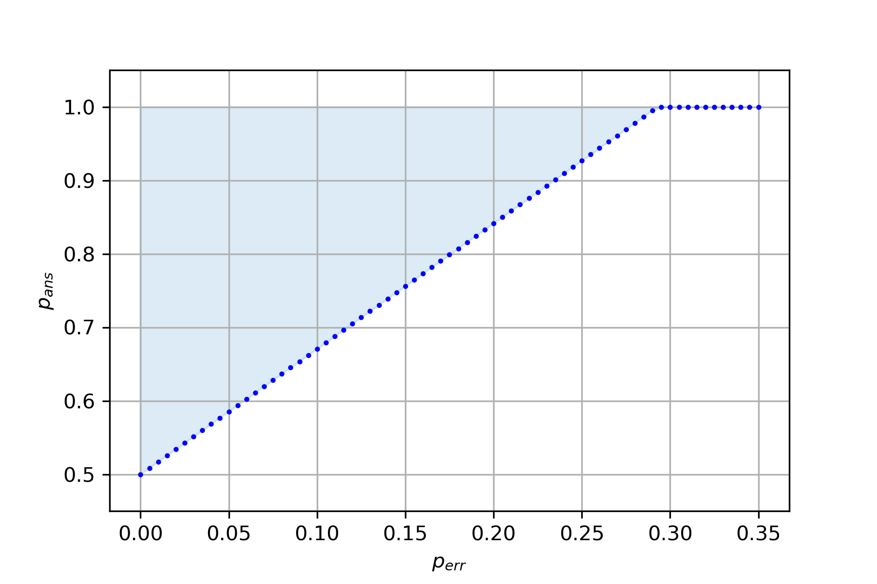
Figure 10: Solution of the first level of the NPA hierarchy of the SPD (65) (blue dots) and the light blue area corresponds to a $SSR$.

From the solutions of (65), represented in Fig. 10, we find that for $p_{err}\approx 0.2929$, an eavesdropper Eve controlling Bob’s device can always answer without being caught, implying that the probability of winning such a MoE game is upper bounded by $0.7071$. Therefore, the protocol, for $n=1$, can tolerate a noise at least up to $0.2929$.

7 Discussion

We have studied the $\mathrm{QPV_{BB84}}$ protocol, providing a tight characterization of its security with loss of quantum information and a prover subject to an experimental error under non-entangled attackers that can do LOQC. Since this protocol is secure only for a transmission rate of photons $\eta\geq\frac{1}{2}$, which is still hard for current technology to achieve, we introduced an extension of the protocol more resistant to transmission loss of the quantum information. The new protocol has the advantage, like the $\mathrm{QPV_{BB84}}$ protocol, that only a single qubit is required to be transmitted in per round of the protocol and the honest prover only needs to broadcast classical information, which does not encounter the problems of loss and slow transmission, making it a good candidate for future implementation.

We have also extended our analysis to the lossy version of the $\mathrm{QPV}_{\mathrm{BB84}}^{f}$  protocol, thereby exhibiting a protocol which is secure against attackers sharing an amount of entanglement that scales in the amount of classical information, while the honest parties only need to manipulate a single qubit per round. By showing (partial) loss-tolerance, the resulting (especially multi-basis) protocol will be much easier to implement in practice. The security proof of that protocol still holds identically in case the transmission of the quantum state is slow, but only the classical bits are transmitted fast, which can be experimentally convenient.

We applied the proof techniques used to show security to improve the upper bounds known so far for certain types of monogamy-of-entanglement games and, as a particular application, we improve the security analysis of one-sided device-independent quantum key distribution for the particular case of $n=1$. However, we leave as an open question whether this can be generalized to show security for arbitrary $n$.

Open questions.

A technical question in the QPV setting which we leave open is to obtain a tight finite statistical analysis for these protocols over multiple rounds. It seems intuitively clear that, since honest parties can achieve a better combination of error and response rate than any attacker for any round, the serial repetition of the proposed protocols should be secure – and we indeed expect this to be the case. However, attackers have a choice in what attack strategy to apply every round, and might even gain a slight amount by being adaptive, e.g., play a low-loss low-error round if the attackers had a lucky guess in a previous round. Because of this, finding the technical tools to bounds the best possible attack over many rounds is non-trivial.

The work of Johnston, Mittal, Russo, and Watrous [JMRW16] shows techniques how to handle extended non-local games, such as the monogamy-of-entanglement games, using SDPs. Because our work directly extends the earlier independent partial results of Buhrman, Schaffner, Speelman, and Zbinden [Spe16b, Chapter 5], we use a slightly-different SDP formulation. It would be very interesting to attempt to extend the results from [JMRW16] to extended non-local games where the players are allowed to return ‘loss’ with some probability – and investigate whether their SDP formulation gives equivalent results to ours.

Additionally, we note that (also for the proposed lossy protocols) an exponential gap remains between the entanglement required of the best attack known and the lower bounds we are able to prove. That is, we show security against attackers sharing a linear amount of entanglement, but we only know of an explicit attack whenever the attackers share an exponential number of qubits. More efficient attacks are known for specific functions, such as $f$ computable in logarithmic space [BFSS13] (for a routing version of the protocol, however the technique can easily be adapted), cf. [CM22], but even these take a polynomial amount of entanglement. Closing this gap remains a large and interesting open problem.

A related open question from the other side therefore also remains: It would be helpful to exhibit these linear lower bounds for specific efficiently-computable functions, instead of just showing that the bound holds for most functions.

Appendix A Non-local games and the NPA hierarchy

Let $\mathcal{G}$ be a non-local game where two non-communicating distant parties, Alice and Bob, have respective questions $x\in\mathcal{X}$ and $y\in\mathcal{Y}$, given according to a probability distribution $q(x,y)$, they input their questions in a respective black box, and they get as outputs measurement outcomes $a\in\mathcal{A}$ and $b\in\mathcal{B}$, for $\mathcal{X},\mathcal{Y},\mathcal{A},\mathcal{B}$, finite alphabets. The winning condition is determined by the predicate $f(a,b,x,y)$, taking value 1 if the game is won and 0, otherwise. The behavior of the box is completely characterized by the probability of getting outcomes $a$ and $b$ having measured $x$ and $y$, $p(a,b|x,y)$, and the set of all probabilities, $\{p(a,b|x,y)\}$, encoded in a stochastic matrix $P\in L(\mathbb{R}^{\mathcal{X}}\otimes\mathbb{R}^{\mathcal{Y}},\mathbb{R}^{\mathcal{A}}\otimes\mathbb{R}^{\mathcal{B}})$, where $L$ is the set of linear operators, such that $P(a,b|x,y)=p(a,b|x,y)$, is called behavior. The average winning probability is given by

$$\omega(\mathcal{G})=\sum_{x,y,a,b}q(x,y)f(a,b,x,y)p(a,b|x,y):=\langle K,P\rangle,$$ (66)

where $K$ is the matrix defined as $K(a,b|x,y)=q(x,y)f(a,b,x,y)$.

Definition A.1.

A behavior $P$ is quantum if there exists a pure state $\left|\psi\right\rangle$ in a Hilbert space $\mathcal{H}$, a set of measurement operators $\{A_{a}^{x}\}_{a\in\mathcal{A}}$ for Alice, and a set of measurement operators $\{B_{b}^{y}\}_{b\in\mathcal{B}}$ for Bob such that for all $a\neq a^{\prime}\in\mathcal{A}$ and $b\neq b^{\prime}\in\mathcal{B}$,

$$p(a,b|x,y)=\left\langle\psi\right|A_{a}^{x}B_{b}^{y}\left|\psi\right\rangle,$$ (67)

with the measurement operators satisfying

1. $A_{a}^{x\dagger}=A_{a}^{x}$ and $B_{b}^{y\dagger}=B_{b}^{y}$,

2. $A_{a}^{x}A_{a^{\prime}}^{x}$=0 and $B_{b}^{y}B_{b^{\prime}}^{y}=0$,

3. $\sum_{a\in\mathcal{A}}A_{a}^{x}=\mathbb{I}$ and $\sum_{b\in\mathcal{B}}B_{b}^{y}=\mathbb{I}$,

4. $[A_{a}^{x},B_{b}^{y}]=0$.

The tuple $\mathcal{S}=\{\left|\psi\right\rangle,A_{a}^{x},B_{b}^{y}\}_{x\in\mathcal{X},y\in\mathcal{Y},a\in\mathcal{A},b\in\mathcal{B}}$ is called strategy, and the set of all quantum behaviors is denoted by $\mathcal{Q}$. Abusing notation, we will denote $\mathcal{S}\in\mathcal{Q}$.

Similarly, a behavior $P$ belongs to the set of quantum behaviors $\mathcal{Q}^{\prime}$ if the Hilbert space can be written as $\mathcal{H}=\mathcal{H}_{A}\otimes\mathcal{H}_{B}$ and the measurement operators for Alice and Bob act on $\mathcal{H}_{A}$ and $\mathcal{H}_{B}$, respectively, and fulfil the same constraints as in Definition A.1 (notice that commutativity is immediately implied because of the tensor product structure). Notice that by construction, $\mathcal{Q}^{\prime}\subseteq\mathcal{Q}$ and for finite dimensional Hilbert space, they turn out to be identical [NPA08].

Therefore, the behaviors (67) can be obtained via tensor product structure, which is the case that we will consider from now on. The maximum winning probability using a quantum behavior $P$ is given by

$$\omega^{*}(\mathcal{G})=\sup_{P\in\mathcal{Q}}\langle K,P\rangle.$$ (68)

In [NPA08], Navascués, Pironio and Acín (NPA) introduced an infinite hierarchy of conditions satisfied by any set of quantum correlations $\mathcal{Q}$ that, each of them, can be tested using semidefinite programming, where the set $\mathcal{Q}$ is fully characterized by it. First, consider the Gram matrix $G$ of the vectors

$$\mathcal{T}=\{\left|\psi\right\rangle\}\cup\{A_{a}^{x}\left|\psi\right\rangle:a\in\mathcal{A},x\in\mathcal{X}\}\cup\{B_{b}^{y}\left|\psi\right\rangle:b\in\mathcal{B},y\in\mathcal{Y}\},$$ (69)

then $G$ contains all the values appearing in $P$. The matrix $G$, which we naturally label by the set $\mathcal{T}$, and its entreis fulfill the following constraints:

1. $G$ is positive semidefinite,

   $$G\succeq 0.$$ (70)

2. $\left|\psi\right\rangle$ is a normalized state, thus $\left\langle\psi\lvert\psi\right\rangle=1$, i.e., $G_{0,0}=1$.

3. $A_{a}^{x}$ and $B_{b}^{y}$ are projector operators, therefore, $\forall x\in\mathcal{X}$, $\forall y\in\mathcal{Y}$, $\forall a\neq a^{\prime}\in\mathcal{A}$, $\forall b\neq b^{\prime}\in\mathcal{B}$ and $\forall T\in\mathcal{T}$:

   1. $\langle A_{a}^{x}A_{a}^{x}\rangle=\langle A_{a}^{x}\rangle$ and likewise for $B_{b}^{y}$.

   2. Because of completeness of measurements:

      $$\begin{split}&\sum_{a\in\mathcal{A}}\langle\psi|A_{a}^{x}T\rangle=\langle\psi|T\rangle,\hskip 28.45274pt\sum_{a\in\mathcal{A}}\langle TA_{a}^{x}|\psi\rangle=\langle T|\psi\rangle,\\ &\sum_{b\in\mathcal{B}}\langle\psi|B_{b}^{y}T\rangle=\langle\psi|T\rangle,\hskip 28.45274pt\sum_{b\in\mathcal{B}}\langle TB_{b}^{y}|\psi\rangle=\langle T|\psi\rangle.\end{split}$$ (71)

   3. Because they are orthogonal projections: $\langle A_{a}^{x}A_{a^{\prime}}^{x}\rangle=0=\langle B_{b}^{y}B_{b^{\prime}}^{y}\rangle$.

   4. Because they commute: $\langle A_{a}^{x}B_{b}^{y}\rangle=\langle B_{b}^{y}A_{a}^{x}\rangle$.

Define

$$\mathcal{Q}_{1}=\{P\textrm{ }\mid\textrm{ }\exists\textrm{ }G\textrm{ fulfilling 1.-3. and }P(a,b|x,y)=\langle A_{a}^{x}B_{b}^{y}\rangle\}\subset L(\mathbb{R}^{\mathcal{X}}\otimes\mathbb{R}^{\mathcal{Y}},\mathbb{R}^{\mathcal{A}}\otimes\mathbb{R}^{\mathcal{B}}),$$ (72)

By construction, $\mathcal{Q}_{1}\supseteq\mathcal{Q}$ and therefore,

$$\omega^{*}(\mathcal{G})=\sup_{P\in\mathcal{Q}}\langle K,P\rangle\leq\sup_{P\in\mathcal{Q}_{1}}\langle K,P\rangle.$$ (73)

Define the Hermitian operator $H$ as the matrix whose entries are $H(xa,yb)=H(yb,xa)=\frac{1}{2}q(x,y)f(a,b,x,y)$ for all $x\in\mathcal{X}$, $y\in\mathcal{Y}$, $a\in\mathcal{A}$, $b\in\mathcal{B}$ and all the other entries are $0$, so that $\langle K,P\rangle=\langle H,G\rangle$. The semidefinite program over all positive semidefinite matrices $G$ satisfying items $1$ to $3$ is the first level of the NPA hierarchy. The level $l$ of the hierarchy, $\mathcal{Q}_{l}$, see [NPA08] for a formal definition, is built considering the Gram matrix of the vectors of the Gram matrix of level $l-1$ and vectors corresponding to $l$ degree products of the projection operators. By construction, $\mathcal{Q}_{l}\supseteq\mathcal{Q}$.

Theorem A.2.

[NPA08] The NPA hierarchy converges to the set of quantum behaviors:

$$\mathcal{Q}=\bigcap_{\ell\in\mathbb{N}}\mathcal{Q}_{\ell}.$$ (74)

Appendix B Proof of Proposition 4.2

Combining both expressions in (16), using the properties of the projectors and equation (47), we obtain the inequality

$$\langle V_{1}^{x}A_{0}^{x}B_{0}^{x}\rangle+\langle V_{0}^{x}A_{1}^{x}B_{1}^{x}\rangle\leq p_{err}(\langle A_{0}^{x}B_{0}^{x}\rangle+\langle A_{1}^{x}B_{1}^{x}\rangle).$$ (75)

Because of (47), from (75) we get

$$\langle V_{1}^{x}A_{0}^{x}\rangle+\langle V_{0}^{x}A_{1}^{x}\rangle\leq p_{err}(\langle A_{0}^{x}B_{0}^{x}\rangle+\langle A_{1}^{x}B_{1}^{x}\rangle),$$ (76)

$$\langle V_{1}^{x}B_{0}^{x}\rangle+\langle V_{0}^{x}B_{1}^{x}\rangle\leq p_{err}(\langle A_{0}^{x}B_{0}^{x}\rangle+\langle A_{1}^{x}B_{1}^{x}\rangle),$$ (77)

$$\langle V_{1}^{x}A_{0}^{x}\rangle+\langle V_{0}^{x}B_{1}^{x}\rangle\leq p_{err}(\langle A_{0}^{x}B_{0}^{x}\rangle+\langle A_{1}^{x}B_{1}^{x}\rangle),$$ (78)

$$\langle V_{1}^{x}B_{0}^{x}\rangle+\langle V_{0}^{x}A_{1}^{x}\rangle\leq p_{err}(\langle A_{0}^{x}B_{0}^{x}\rangle+\langle A_{1}^{x}B_{1}^{x}\rangle).$$ (79)

We will use it to find linear constraints on the entries of the gram matrix $G$ corresponding to $\langle A_{a}^{x}B_{b}^{x^{\prime}}\rangle$. Consider

$$\begin{split}2\langle A_{a}^{x}B_{b}^{x^{\prime}}\rangle&=2\langle\mathbb{I}\otimes A_{a}^{x}\otimes B_{b}^{x^{\prime}}\rangle=\langle(V_{a}^{x}+V_{1-a}^{x})A_{a}^{x}B_{b}^{x^{\prime}}\rangle+\langle(V_{b}^{x^{\prime}}+V_{1-b}^{x^{\prime}})A_{a}^{x}B_{b}^{x^{\prime}}\rangle\\ &=\langle(V_{a}^{x}+V_{b}^{x^{\prime}})A_{a}^{x}B_{b}^{x^{\prime}}\rangle+\langle V_{1-a}^{x}A_{a}^{x}B_{b}^{x^{\prime}}\rangle+\langle V_{1-b}^{x^{\prime}}A_{a}^{x}B_{b}^{x^{\prime}}\rangle,\end{split}$$ (80)

then, summing over $a$ and $b$, we get

$$\begin{split}2\sum_{ab}\langle A_{a}^{x}B_{b}^{x^{\prime}}\rangle&=\sum_{ab}\langle((V_{a}^{x}+V_{b}^{x^{\prime}}))A_{a}^{x}B_{b}^{x^{\prime}}\rangle+\langle V_{1}^{x}A_{0}^{x}(B_{0}^{x^{\prime}}+B_{1}^{x^{\prime}})\rangle+\langle V_{0}^{x}A_{1}^{x}(B_{0}^{x^{\prime}}+B_{1}^{x^{\prime}})\rangle+\\ &\langle V_{1}^{x^{\prime}}(A_{0}^{x}+A_{1}^{x})B_{0}^{x^{\prime}}\rangle+\langle V_{0}^{x^{\prime}}(A_{0}^{x}+A_{1}^{x})B_{1}^{x^{\prime}}\rangle\\ &\leq\sum_{ab}\langle((V_{a}^{x}+V_{b}^{x^{\prime}}))A_{a}^{x}B_{b}^{x^{\prime}}\rangle+\langle V_{1}^{x}A_{0}^{x}\rangle+\langle V_{0}^{x}A_{1}^{x}\rangle+\langle V_{1}^{x^{\prime}}B_{0}^{x^{\prime}}\rangle+\langle V_{0}^{x^{\prime}}B_{1}^{x^{\prime}}\rangle,\end{split}$$ (81)

where we used that $A_{0}^{x}+A_{1}^{x}\preceq\mathbb{I}$ and $B_{0}^{x^{\prime}}+B_{1}^{x^{\prime}}\preceq\mathbb{I}$. Then, using (76) and (77), we recover (48).

On the other hand, recall that

$$V_{a}^{x}=\left|a_{x}\rangle\langle a_{x}\right|\textrm{ and }V_{b}^{x^{\prime}}=\left|b_{x^{\prime}}\rangle\langle b_{x^{\prime}}\right|,$$ (82)

and we can write

$$\begin{split}&\left|a_{x}\right\rangle=\alpha_{0}^{a}\left|0_{x^{\prime}}\right\rangle+\alpha_{1}^{a}\left|1_{x^{\prime}}\right\rangle\\ &\left|b_{x^{\prime}}\right\rangle=\beta_{0}^{b}\left|0_{x}\right\rangle+\beta_{1}^{b}\left|1_{x}\right\rangle,\\ \end{split}$$ (83)

where $\alpha_{i}^{a}=\left\langle i_{x^{\prime}}\lvert a_{x}\right\rangle$ and $\beta_{j}^{b}=\left\langle j_{x}\lvert b_{x^{\prime}}\right\rangle$, where the dependence on $x$ and $x^{\prime}$ is omitted for simplicity. We write the projectors (82) in the other basis in such a way that

$$\begin{split}&V_{a}^{x}=\lvert\alpha_{0}^{a}\rvert^{2}V_{0}^{x^{\prime}}+\lvert\alpha_{1}^{a}\rvert^{2}V_{1}^{x^{\prime}}+\alpha_{0}^{a}\alpha_{1}^{a*}\left|0_{x^{\prime}}\rangle\langle 1_{x^{\prime}}\right|+\alpha_{0}^{a*}\alpha_{1}^{a}\left|1_{x^{\prime}}\rangle\langle 0_{x^{\prime}}\right|,\\ &V_{b}^{x^{\prime}}=\lvert\beta_{0}^{b}\rvert^{2}V_{0}^{x}+\lvert\beta_{1}^{b}\rvert^{2}V_{1}^{x}+\beta_{0}^{b}\beta_{1}^{b*}\left|0_{x}\rangle\langle 1_{x}\right|+\beta_{0}^{b*}\beta_{1}^{b}\left|1_{x}\rangle\langle 0_{x}\right|.\end{split}$$ (84)

Plugging (84) in (80), summing (80) and summing over $a$ and $b$ in $\{0,1\}$,

$$\begin{split}&4\sum_{a,b}\langle A_{a}^{x}B_{b}^{x^{\prime}}\rangle=\\ &\langle((1+\lvert\beta_{0}^{0}\rvert^{2})V_{0}^{x}+(1+\lvert\alpha_{0}^{0}\rvert^{2})V_{0}^{x^{\prime}}+\beta_{0}^{0}\beta_{1}^{0*}\left|0_{x}\rangle\langle 1_{x}\right|+\beta_{0}^{0*}\beta_{1}^{0}\left|1_{x}\rangle\langle 0_{x}\right|+\\ &\alpha_{0}^{0}\alpha_{1}^{0*}\left|0_{x^{\prime}}\rangle\langle 1_{x^{\prime}}\right|+\alpha_{0}^{0*}\alpha_{1}^{0}\left|1_{x^{\prime}}\rangle\langle 0_{x^{\prime}}\right|)A_{0}^{x}B_{0}^{x^{\prime}}\rangle+(2+\lvert\beta_{1}^{0}\rvert^{2})\langle V_{1}^{x}A_{0}^{x}B_{0}^{x^{\prime}}\rangle+(2+\lvert\alpha_{1}^{0}\rvert^{2})\langle V_{1}^{x^{\prime}}A_{0}^{x}B_{0}^{x^{\prime}}\rangle+\\ &\langle((1+\lvert\beta_{0}^{1}\rvert^{2})V_{0}^{x}+(1+\lvert\alpha_{1}^{0}\rvert^{2})V_{1}^{x^{\prime}}+\beta_{0}^{1}\beta_{1}^{1*}\left|0_{x}\rangle\langle 1_{x}\right|+\beta_{0}^{1*}\beta_{1}^{1}\left|1_{x}\rangle\langle 0_{x}\right|+\\ &\alpha_{0}^{0}\alpha_{1}^{0*}\left|0_{x^{\prime}}\rangle\langle 1_{x^{\prime}}\right|+\alpha_{0}^{0*}\alpha_{1}^{0}\left|1_{x^{\prime}}\rangle\langle 0_{x^{\prime}}\right|)A_{0}^{x}B_{1}^{x^{\prime}}\rangle+(2+\lvert\beta_{1}^{1}\rvert^{2})\langle V_{1}^{x}A_{0}^{x}B_{1}^{x^{\prime}}\rangle+(2+\lvert\alpha_{0}^{0}\rvert^{2})\langle V_{0}^{x^{\prime}}A_{0}^{x}B_{1}^{x^{\prime}}\rangle+\\ &\langle((1+\lvert\beta_{1}^{0}\rvert^{2})V_{1}^{x}+(1+\lvert\alpha_{0}^{1}\rvert^{2})V_{0}^{x^{\prime}}+\beta_{0}^{0}\beta_{1}^{0*}\left|0_{x}\rangle\langle 1_{x}\right|+\beta_{0}^{0*}\beta_{1}^{0}\left|1_{x}\rangle\langle 0_{x}\right|+\\ &\alpha_{0}^{1}\alpha_{1}^{1*}\left|0_{x^{\prime}}\rangle\langle 1_{x^{\prime}}\right|+\alpha_{0}^{1*}\alpha_{1}^{1}\left|1_{x^{\prime}}\rangle\langle 0_{x^{\prime}}\right|)A_{1}^{x}B_{0}^{x^{\prime}}\rangle+(2+\lvert\beta_{0}^{0}\rvert^{2})\langle V_{0}^{x}A_{1}^{x}B_{0}^{x^{\prime}}\rangle+(2+\lvert\alpha_{1}^{1}\rvert^{2})\langle V_{1}^{x^{\prime}}A_{1}^{x}B_{0}^{x^{\prime}}\rangle+\\ &\langle((1+\lvert\beta_{1}^{1}\rvert^{2})V_{1}^{x}+(1+\lvert\alpha_{1}^{1}\rvert^{2})V_{1}^{x^{\prime}}+\beta_{0}^{1}\beta_{1}^{1*}\left|0_{x}\rangle\langle 1_{x}\right|+\beta_{0}^{1*}\beta_{1}^{1}\left|1_{x}\rangle\langle 0_{x}\right|+\\ &\alpha_{0}^{1}\alpha_{1}^{1*}\left|0_{x^{\prime}}\rangle\langle 1_{x^{\prime}}\right|+\alpha_{0}^{1*}\alpha_{1}^{1}\left|1_{x^{\prime}}\rangle\langle 0_{x^{\prime}}\right|)A_{1}^{x}B_{1}^{x^{\prime}}\rangle+(2+\lvert\beta_{0}^{1}\rvert^{2})\langle V_{0}^{x}A_{1}^{x}B_{1}^{x^{\prime}}\rangle+(2+\lvert\alpha_{0}^{1}\rvert^{2})\langle V_{0}^{x^{\prime}}A_{1}^{x}B_{1}^{x^{\prime}}\rangle\\ \end{split}$$ (85)

Using that $A_{0}^{x}+A_{1}^{x}\preceq\mathbb{I}$ and $B_{0}^{x^{\prime}}+B_{1}^{x^{\prime}}\preceq\mathbb{I}$ and (76) and (77), as in derivation of (48), and bounding the terms that do not correspond to $\langle V_{1-a}A_{a}B_{b}\rangle$ or $\langle V_{1-b}^{\prime}A_{a}B_{b}\rangle$ by the operator norm, we obtain (49).

Appendix C Proof of Proposition 6.1

Combining both expressions in (63), using the properties of the projectors and equation (62), we obtain the inequality, for $e,b\in\{0,1\}$

$$\langle V_{0}^{x}E_{0}^{x}B_{1}^{x}\rangle+\langle V_{1}^{x}E_{1}^{x}B_{0}^{x}\rangle\leq p_{err}\sum_{e,b}\langle E_{e}^{x}B_{b}^{x}\rangle.$$ (86)

Because of (62), from (86) we get

$$\langle V_{0}^{x}B_{1}^{x}\rangle+\langle V_{1}^{x}B_{0}^{x}\rangle\leq p_{err}\sum_{e,b}\langle E_{e}^{x}B_{b}^{x}\rangle.$$ (87)

In an analogy with (80), consider

$$2\langle E_{e}^{x}B_{b}^{x^{\prime}}\rangle=\langle(V_{e}^{x}+V_{b}^{x^{\prime}})E_{e}^{x}B_{b}^{x^{\prime}}\rangle+\langle V_{1-e}^{x}E_{e}^{x}B_{b}^{x^{\prime}}\rangle+\langle V_{1-b}^{x^{\prime}}E_{e}^{x}B_{b}^{x^{\prime}}\rangle,$$ (88)

because of (62), $\langle V_{1-e}^{x}E_{e}^{x}B_{b}^{x^{\prime}}\rangle=0$, summing (88) over $e,b\in\{0,1\}$, using $A_{0}^{x}+A_{1}^{x}\preceq\mathbb{I}$ applying (87), we recover (64).

References

- [ABSL22] Rene Allerstorfer, Harry Buhrman, Florian Speelman, and Philip Verduyn Lunel. On the role of quantum communication and loss in attacks on quantum position verification. arXiv preprint arXiv:2208.04341, 2022.
- [ABSV21] Rene Allerstorfer, Harry Buhrman, Florian Speelman, and Philip Verduyn Lunel. Towards practical and error-robust quantum position verification. arXiv preprint arXiv:2106.12911, 2021.
- [AKB06] Tomothy Spiller Adrian Kent, William Munro and Raymond Beausoleil. Tagging systems. us patent nr 2006/0022832. 2006.
- [BB84] Charles H. Bennett and Gilles Brassard. Quantum cryptography: public key distribution and coin tossing. Proc. IEEE Int. Conf. on Computers, Systems, and Signal Process (Bangalore) (Piscataway, NJ: IEEE), 1984.
- [BBM92] Charles H. Bennett, Gilles Brassard, and N. David Mermin. Quantum cryptography without Bell’s theorem. Phys. Rev. Lett., 68:557–559, Feb 1992.
- [BCF+14] Harry Buhrman, Nishanth Chandran, Serge Fehr, Ran Gelles, Vipul Goyal, Rafail Ostrovsky, and Christian Schaffner. Position-based quantum cryptography: Impossibility and constructions. SIAM Journal on Computing, 43(1):150–178, jan 2014.
- [BCP+14] Nicolas Brunner, Daniel Cavalcanti, Stefano Pironio, Valerio Scarani, and Stephanie Wehner. Bell nonlocality. Rev. Mod. Phys., 86:419–478, Apr 2014.
- [BCS22] Andreas Bluhm, Matthias Christandl, and Florian Speelman. A single-qubit position verification protocol that is secure against multi-qubit attacks. Nature Physics, pages 1–4, 2022.
- [BFSS13] Harry Buhrman, Serge Fehr, Christian Schaffner, and Florian Speelman. The garden-hose model. In Proceedings of the 4th conference on Innovations in Theoretical Computer Science - ITCS '13. ACM Press, 2013.
- [BK11] Salman Beigi and Robert König. Simplified instantaneous non-local quantum computation with applications to position-based cryptography. New Journal of Physics, 13(9):093036, sep 2011.
- [CGMO09] Nishanth Chandran, Vipul Goyal, Ryan Moriarty, and Rafail Ostrovsky. Position based cryptography. In Advances in Cryptology - CRYPTO 2009, 29th Annual International Cryptology Conference, volume 5677 of Lecture Notes in Computer Science, pages 391–407. Springer, 2009.
- [CHTW04] Richard Cleve, Peter Hoyer, Ben Toner, and John Watrous. Consequences and limits of nonlocal strategies, 2004.
- [CL15] Kaushik Chakraborty and Anthony Leverrier. Practical position-based quantum cryptography. Physical Review A, 92(5), nov 2015.
- [CM22] Sam Cree and Alex May. Code-routing: a new attack on position-verification. arXiv preprint arXiv:2202.07812, 2022.
- [DC22] Kfir Dolev and Sam Cree. Non-local computation of quantum circuits with small light cones. arXiv preprint arXiv:2203.10106, 2022.
- [Dol19] Kfir Dolev. Constraining the doability of relativistic quantum tasks. arXiv preprint arXiv:1909.05403, 2019.
- [EFS] Llorenç Escolà-Farràs and Florian Speelman. https://github.com/llorensescola/QPV_NPA_hierarchy.
- [GC19] Alvin Gonzales and Eric Chitambar. Bounds on instantaneous nonlocal quantum computation. IEEE Transactions on Information Theory, 66(5):2951–2963, 2019.
- [GLW16] Fei Gao, Bin Liu, and QiaoYan Wen. Quantum position verification in bounded-attack-frequency model. SCIENCE CHINA Physics, Mechanics & Astronomy, 59(11):1–11, 2016.
- [JKPPG22] Marius Junge, Aleksander M Kubicki, Carlos Palazuelos, and David Pérez-García. Geometry of banach spaces: a new route towards position based cryptography. Communications in Mathematical Physics, pages 1–54, 2022.
- [JMRW16] Nathaniel Johnston, Rajat Mittal, Vincent Russo, and John Watrous. Extended non-local games and monogamy-of-entanglement games. Proceedings of the Royal Society A: Mathematical, Physical and Engineering Sciences, 472(2189):20160003, may 2016.
- [KMS11] Adrian Kent, William J. Munro, and Timothy P. Spiller. Quantum tagging: Authenticating location via quantum information and relativistic signaling constraints. Physical Review A, 84(1), Jul 2011.
- [LL11] Hoi-Kwan Lau and Hoi-Kwong Lo. Insecurity of position-based quantum-cryptography protocols against entanglement attacks. Physical Review A, 83(1), jan 2011.
- [LLQ21] Jiahui Liu, Qipeng Liu, and Luowen Qian. Beating classical impossibility of position verification. arXiv preprint arXiv:2109.07517, 2021.
- [LT91] Michel Ledoux and Michel Talagrand. Probability in Banach Spaces: Isoperimetry and Processes, volume 23 of A Series of Modern Surveys in Mathematics Series. Springer, Berlin, 1991.
- [LXS+16] Charles Ci Wen Lim, Feihu Xu, George Siopsis, Eric Chitambar, Philip G Evans, and Bing Qi. Loss-tolerant quantum secure positioning with weak laser sources. Physical Review A, 94(3):032315, 2016.
- [MJAS77] F. Jessie MacWilliams and Neil. J. A. Sloane. The Theory of Error-Correcting Codes, volume 16 of NorthHolland Mathematical Library. North-Holland, 1977.
- [NC11] Michael A. Nielsen and Isaac L. Chuang. Quantum Computation and Quantum Information: 10th Anniversary Edition. Cambridge University Press, 2011.
- [NFLR21] Dominik Niemietz, Pau Farrera, Stefan Langenfeld, and Gerhard Rempe. Nondestructive detection of photonic qubits. Nature, 591(7851):570–574, mar 2021.
- [NPA08] Miguel Navascués, Stefano Pironio, and Antonio Acín. A convergent hierarchy of semidefinite programs characterizing the set of quantum correlations. New Journal of Physics, 10(7):073013, Jul 2008.
- [QS15] Bing Qi and George Siopsis. Loss-tolerant position-based quantum cryptography. Physical Review A, 91(4), Apr 2015.
- [RG15] Jérémy Ribeiro and Frédéric Grosshans. A tight lower bound for the bb84-states quantum-position-verification protocol, 2015.
- [Spe16a] Florian Speelman. Instantaneous non-local computation of low T-depth quantum circuits. In 11th Conference on the Theory of Quantum Computation, Communication and Cryptography (TQC 2016). Schloss Dagstuhl-Leibniz-Zentrum fuer Informatik, 2016.
- [Spe16b] Florian Speelman. Position-based quantum cryptography and catalytic computation. PhD thesis, University of Amsterdam, 2016.
- [TFKW13] Marco Tomamichel, Serge Fehr, Jędrzej Kaniewski, and Stephanie Wehner. A monogamy-of-entanglement game with applications to device-independent quantum cryptography. New Journal of Physics, 15(10):103002, Oct 2013.
- [Unr14] Dominique Unruh. Quantum position verification in the random oracle model. In Juan A. Garay and Rosario Gennaro, editors, Advances in Cryptology – CRYPTO 2014, pages 1–18, Berlin, Heidelberg, 2014. Springer Berlin Heidelberg.
- [Weh06] Stephanie Wehner. Tsirelson bounds for generalized clauser-horne-shimony-holt inequalities. Physical Review A, 73(2), feb 2006.
- [Wei] Eric W. Weisstein. Sphere point picking. from mathworld–a wolfram web resource. https://mathworld.wolfram.com/spherepointpicking.html.
- [Wit15] Peter Wittek. Algorithm 950. ACM Transactions on Mathematical Software, 41(3):1–12, jun 2015.
- [WZ82] William K. Wootters and Wojciech Zurek. A single quantum cannot be cloned. Nature, 299:802–803, 1982.