Network Analysis of Count Data from Mixed Populations

\nameJunjie Tang \emailjunjie.tang@pku.edu.cn
\nameChanghu Wang \emailwangch156@pku.edu.cn
\nameFeiyi Xiao \emailxiaofeiyi1217@pku.edu.cn
\nameRuibin Xi \emailruibinxi@math.pku.edu.cn
\addrSchool of Mathematical Sciences
Peking University
Beijing, 100871, CHN
Abstract

In applications such as gene regulatory network analysis based on single-cell RNA sequencing data, samples often come from a mixture of different populations and each population has its own unique network. Available graphical models often assume that all samples are from the same population and share the same network. One has to first cluster the samples and use available methods to infer the network for every cluster separately. However, this two-step procedure ignores uncertainty in the clustering step and thus could lead to inaccurate network estimation. Motivated by these applications, we consider the mixture Poisson log-normal model for network inference of count data from mixed populations. The latent precision matrices of the mixture model correspond to the networks of different populations and can be jointly estimated by maximizing the lasso-penalized log-likelihood. Under rather mild conditions, we show that the mixture Poisson log-normal model is identifiable and has the positive definite Fisher information matrix. Consistency of the maximum lasso-penalized log-likelihood estimator is also established. To avoid the intractable optimization of the log-likelihood, we develop an algorithm called VMPLN based on the variational inference method. Comprehensive simulation and real single-cell RNA sequencing data analyses demonstrate the superior performance of VMPLN.

Keywords: Graphical model, Identifiability, Mixed model, Single-cell RNA sequencing, Variational inference

1 Introduction

Graphical models (Drton and Maathuis, 2017) such as the Gaussian graphical model (Meinshausen and Bühlmann, 2006; Friedman et al., 2008) have been widely applied to many different fields for identifying key interactions between random variables (Farasat et al., 2015; Wille et al., 2004; Dobra and Lenkoski, 2011). These graphical models usually assume that all samples, or at least the samples under a known condition, are sampled from the same population and thus have the same network. However, in applications such as the recent single-cell RNA sequencing (scRNA-seq) studies (Aibar et al., 2017; Specht and Li, 2017; Chan et al., 2017; Aibar et al., 2017; Song et al., 2022), samples often come from a mixture of different populations and each population has its own unique network. In scRNA-seq studies, samples are single cells of different cell types and each cell type has its unique gene regulatory network. Gene expressions of single cells are measured as counts of short reads or unique molecular identifiers. Because the cell identities are unknown, one has to first assign single cells to different cell types (e.g. by clustering) and then estimates the gene regulatory networks using available methods. This two-step procedure can provide accurate network estimation if different populations are well separated. If, instead, different populations have a higher mixing degree, a large proportion of samples cannot be confidently assigned with a label and the incorrect label assignment could seriously influence the performance of network inference (See Figure 1 for an example).

Refer to caption
Figure 1: An example of data from a two-dimensional mixture Gaussian distribution. We sample 2000 observations from the Gaussian mixture model $0.5\ \mbox{N}\left(\mu=(0,0),\Sigma=\Theta_{1}^{-1}\right)+0.5\ \mbox{N}\left(\mu=(1.7,1.7),\Sigma=\Theta_{2}^{-1}\right)$. The diagonal elements of precision matrices $\Theta_{1}$ and $\Theta_{2}$ are 1, and the non-diagonal elements of $\Theta_{1}$ and $\Theta_{2}$ are 0 and $-0.3$, respectively. (a) The scatter plot of the 2000 samples with true labels (red: population 1, blue: population 2). Using the true label, as expected, samples in population 1 demonstrate a partial correlation very close to 0, and samples in population 2 have a large nonzero partial correlation (0.30). (b) The samples are first clustered using the K-means algorithm. Partial correlations are calculated for each cluster and are far away from the true partial correlations, which would lead to incorrect network estimates. (c) Parameters are estimated by maximizing the likelihood of the mixture Gaussian distribution. The estimates of the partial correlations are now close to the true values.

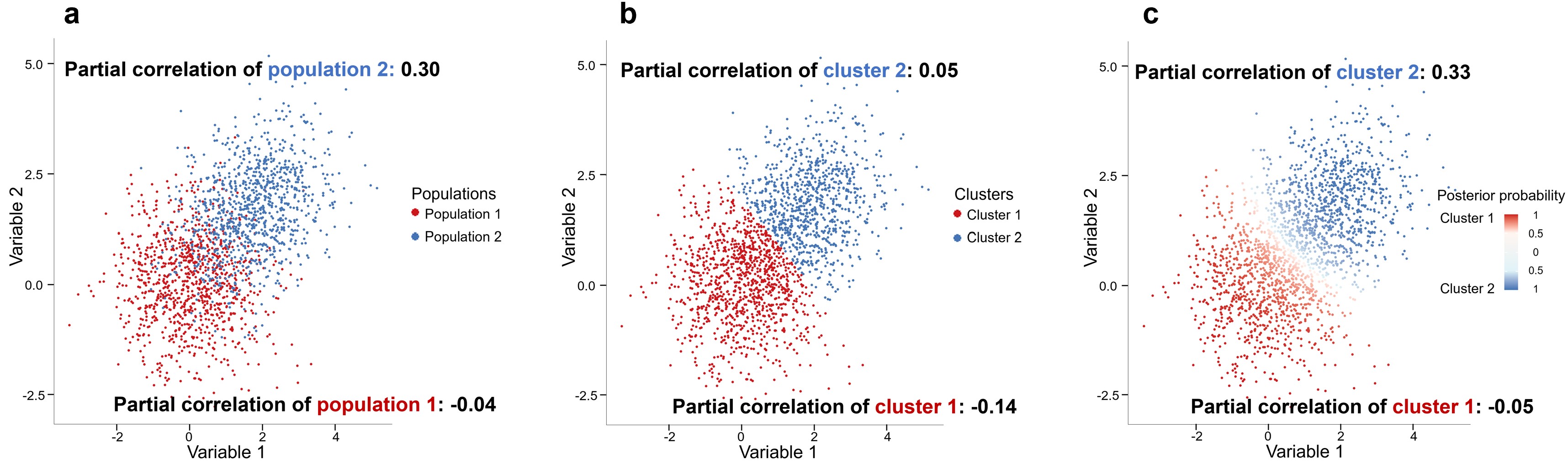
Motivated by the gene regulatory network inference problem in scRNA-seq studies, we consider developing a network inference method for count data from mixed populations using mixture models. One major advantage of mixture models for network inference is that sample identities need not be predetermined before network inference. Instead, mixture models can allow joint analyses of clustering and network inference, and thus could give better network estimation when different populations are poorly separated (See Figure 1 for an example). Available graphical models for count data include Poisson graphical models and their extensions (Yang et al., 2012; Allen and Liu, 2013), negative binomial graphical models (Park et al., 2021) and Poisson log-normal models (Wu et al., 2018; Chiquet et al., 2019; Silva et al., 2019). The Poisson and negative binomial graphical models can only allow negative interactions, and the extension of the Poisson graphical models have no explicit form of the joint distribution and cannot adequately account for over-dispersion in the data, such as in the scRNA-seq data (Ziegenhain et al., 2017). We therefore consider the mixture of Poisson log-normal models for network inference of count data from mixed populations.

A non-negative integer random vector $Y=(Y_{1},\dots,Y_{p})^{T}\in\mathbb{R}^{p}$ follows a Poisson log-normal distribution, if conditional on a latent normal random vector $X=(X_{1},\dots,X_{p})^{T}\sim\mbox{N}(\mu,\Sigma)$, each element $Y_{j}$ of $Y$ independently follows the univariate Poisson distribution $\mbox{Poisson}\left\{\exp(X_{j})\right\}$ ($j=1,\dots,p$). Similar to the Gaussian graphical model, the network of the Poisson log-normal model is the precision matrix $\Theta={\Sigma}^{-1}$ of the latent variable $X$. The mixture Poisson log-normal model is a mixture of $G$ different Poisson log-normal models, and the underlying $G$ latent precision matrices are the networks of different populations. Assuming that the networks are sparse, we can maximize the lasso-penalized log-likelihood of the mixture Poisson log-normal model to estimate the networks. The mixture Poisson log-normal model has been used for clustering count data (Silva et al., 2019) and EM algorithms coupled with MCMC steps are developed to maximize its computational intractable log-likelihood. However, theoretical properties of the mixture Poisson log-normal model are not studied, and EM algorithms with MCMC steps are computationally very expensive.

Here, we propose to use these mixture models for network inference. We establish the basic properties of the mixture Poisson log-normal model including its identifiability and the positive definiteness of its Fisher information matrix. We further show that the network estimator by maximizing the lasso-penalized log-likelihood is consistent. All technical proofs are in appendix Section A. We adopt the variational inference approach (Jordan et al., 1999; Wainwright et al., 2008) and develop a more efficient algorithm called VMPLN for the network inference. We compare VMPLN with popular graphical methods and state-of-the-art gene regulatory network inference methods using simulation and real data analyses. We also demonstrate an application of VMPLN to a large scRNA-seq dataset from patients infected with severe acute respiratory syndrome coronavirus 2 (SARS-CoV-2). All data used and corresponding source codes are available and can be accessed at https://doi.org/10.5281/zenodo.7069698.

2 Model and Theoretical Properties

In this section, we describe the mixture Poisson log-normal model for network inference of count data from mixed populations, and then establish the theoretical properties of the mixture Poisson log-normal model as well as the consistency of network estimator by maximizing the lasso-penalized log-likelihood.

2.1 The Mixture Poisson Log-normal Model of Count data from Mixed Populations

Let $Y_{i}=\left(Y_{i1},\dots,Y_{ip}\right)^{T}$ be the $i$th observation ($i=1,\dots,n$), where $Y_{ij}$’s are all non-negative integers. The $n$ samples belong to $G$ different populations. Conditional on latent variables $X_{ij}$, we assume that $Y_{ij}$’s are independent Poisson variables with parameters $\lambda_{ij}=l_{i}\exp\left(X_{ij}\right)$, where $l_{i}$’s are known scaling factors. The underlying population $Z_{i}$ of the $i$th sample follows a multinomial distribution $\mbox{Multinomial}(1,\pi)$, where $\pi=(\pi_{1},\dots,\pi_{G})^{T}$ is the proportion parameter representing the composition of the mixture components. Given $Z_{i}=g$ ($g=1,\dots,G$), the latent vector $X_{i}=\left(X_{i1},\dots,X_{ip}\right)^{T}$ is normally distributed with a mean $\mu_{g}\in\mathbb{R}^{p}$ and a covariance matrix $\Theta_{g}^{-1}$. In summary, the mixture Poisson log-normal model can be written as,

$\displaystyle Y_{i}\mid X_{i}$ $\displaystyle\sim\prod_{j=1}^{p}\mbox{Poisson}\left\{l_{i}\ \exp\left(X_{ij}\right)\right\},$ (1)
$\displaystyle X_{i}\mid Z_{i}=g$ $\displaystyle\sim\mbox{N}\left(\mu_{g},{\Theta_{g}}^{-1}\right),\Theta_{g}\succ 0,$
$\displaystyle Z_{i}$ $\displaystyle\sim\mbox{Multinomial}(1,\pi),$

where $\Theta_{g}\succ 0$ means that $\Theta_{g}$ is positive definite. In scRNA-seq data, $Y_{ij}$ is the observed expression of the $j$th gene in the $i$th cell, $\exp\left(X_{ij}\right)$ represents the underlying “true” expression, and $l_{i}$ is the library size of the $i$th cell and can be readily estimated (Hafemeister and Satija, 2019; Lun et al., 2016).

Denote $\theta=\big{(}\pi,\mu=\{\mu_{g}\}_{g=1}^{G},\Theta=\{\Theta_{g}\}_{g=1}^{G}\big{)}$ as unknown parameters of the model (1). Let $p(Y_{i}\mid X_{i})=\prod_{j=1}^{p}\left[\left\{l_{i}\exp\left(X_{ij}\right)\right\}^{Y_{ij}}\exp\{-l_{i}\exp\left(X_{ij}\right)\}(Y_{ij}!)^{-1}\right]$ be the conditional probability mass function of $Y_{i}$ given $X_{i}$. The conditional density function $p(X_{i}\mid Z_{i};\mu,\Theta)$ of $X_{i}$ given $Z_{i}$ can be written as $p(X_{i}\mid Z_{i};\mu,\Theta)=\prod_{g=1}^{G}\left\{p(X_{i};\mu_{g},\Theta_{g})\right\}^{I\left(Z_{i}=g\right)}$, where $p(\cdot\ ;\mu_{g},\Theta_{g})$ is the density of $\mbox{N}\left(\mu_{g},{\Theta_{g}}^{-1}\right)$. Denote $p(Z_{i};\pi)=\prod_{g=1}^{G}\pi_{g}^{I(Z_{i}=g)}$ as the probability mass function of the multinomial distribution. The log-likelihood of the mixture model (1) is

$$\ell_{n}(\theta)=\sum_{i=1}^{n}\log\left\{p(Y_{i};\theta)\right\}=\sum_{i=1}^{n}\log\iint p(Y_{i}\mid X_{i})p(X_{i}\mid Z_{i};\mu,\Theta)p(Z_{i};\pi)\mathrm{d}X_{i}\mathrm{d}Z_{i}\ ,$$ (2)

where $p(Y_{i};\theta)$ is the marginal probability mass function of $Y_{i}$. The precision matrices $\Theta_{g}$’s represent the population-specific network. Let $\Theta_{g,lm}$ be the $(l,m)$th element of $\Theta_{g}$. The networks are sparse and can be estimated by minimizing the lasso-penalized negative log-likelihood

$$-n^{-1}\ell_{n}(\theta)+\lambda_{n}\sum_{g=1}^{G}\|{\Theta_{g}}\|_{1,\text{ off }},$$ (3)

where $\lambda_{n}>0$ is a tuning parameter and $\|{\Theta_{g}}\|_{1,\text{ off }}=\sum_{l\neq m}|{\Theta_{g,lm}}|$ is the off-diagonal $l_{1}$-norm of $\Theta_{g}$. In the following, we first establish the consistency of the estimator obtained by minimizing (3) and then derive an algorithm for estimating the precision matrices.

2.2 Theoretical Properties

In this section, we always assume that the true means $\mu_{g}^{*}$ and proportions $\pi_{g}^{*}$ ($g=1,\dots,G$) are known. Let $\nu_{g}={\rm vech}(\Theta_{g})$ be the vectorization of the precision matrix $\Theta_{g}$ (appendix Section A.1) and ${\nu}=(\nu_{1}^{\rm T},\ldots,\nu_{G}^{\rm T})^{\rm T}$ . In this case, the log-likelihood $\ell_{n}(\theta)$ can be viewed as a function of ${\nu}$, also denoting as $\ell_{n}(\nu)$, and we consider the estimator $\hat{\nu}_{n}$ that minimizes $-n^{-1}\ell_{n}(\nu)+\lambda_{n}\sum_{g=1}^{G}\|{\Theta_{g}}\|_{1,\text{ off }}$ subject to $\Theta_{g}\succ 0\ (g=1,\dots,G)$. Denote $\nu^{*}$ as the true value of the unknown parameter $\nu$, $S(\nu)=\{i\mid\ \nu_{i}\neq 0\}$ as the support of $\nu$, and $S^{*}=S({\nu}^{*})$. Suppose that $Y$ follows the mixture model (1) with its log-likelihood function $\ell(\nu,Y)$. Denote $\Gamma^{*}=\Gamma(\nu^{*})=-{\rm E}\left\{\partial^{2}\ell(\nu,Y)/\partial\nu\partial\nu^{T}\right\}\mid_{\nu=\nu^{*}}$ as the Fisher information matrix at $\nu^{*}$, and ${\Gamma^{*}}_{T_{1}T_{2}}$ as the submatrix of ${\Gamma^{*}}$ with rows and columns index by sets $T_{1}$ and $T_{2}$, respectively. Before presenting the theoretical properties, we give the following conditions:
Condition C1. The eigenvalues of the precision matrices are bounded in $[m,M]$, where $0<m<M<\infty$.
Condition C2. The scaling factors $l_{i}>0$ ($i=1,\dots,n$) are independent and identically distributed random variables with a bounded support.
Condition C3. The true mean vectors $\mu_{g}^{*}$ ($g=1,\dots,G$) are bounded and different from each other.
Condition C4 (The irrepresentability condition). $||\Gamma^{*}_{{S^{*}}^{c}S^{*}}{(\Gamma^{*}_{S^{*}S^{*}})}^{-1}||_{\infty}<1$.

Denote $\lambda_{min}(\Theta_{g})$ and $\lambda_{max}(\Theta_{g})$ as the minimum and maximum eigenvalue of $\Theta_{g}$. Define $\mathcal{D}=\{{\nu}=(\nu_{1}^{\rm T},\nu_{2}^{\rm T},\ldots,\nu_{G}^{\rm T})^{\rm T}|\leavevmode\nobreak\ \nu_{g}={\rm vech}(\Theta_{g}),m\leq\lambda_{min}(\Theta_{g})\leq\lambda_{max}(\Theta_{g})\leq M\}$ and $\kappa=\lambda_{min}(\Gamma^{*})$ be the minimum eigenvalue of the Fisher information matrix at $\nu^{*}$. Condition C1-C2 are commonly used in the literature (Cai et al., 2011; Li et al., 2020). Condition C3 is to ensure that different components of the mixture model (1) can be distinguished from each other. Under Condition C3, the mixture model (1) is identifiable and its Fisher information matrix $\Gamma^{*}$ is positive definite, and thus $\kappa>0$. The irrepresentability condition C4 is also commonly used (Zhao and Yu, 2006; Ravikumar et al., 2011). Based on the above conditions, we present the theoretical properties of the mixture model (1) and the estimator $\hat{\nu}_{n}$ in the following theorems.

Theorem 1

Under Condition C1-C3, the mixture Poisson log-normal model (1) is identifiable, and its Fisher information matrix $\Gamma^{*}$ at $\nu^{*}$ is positive definite.

Theorem 1 establishes basic properties of the mixture model (1) and ensures that it is well-behaved under rather mild conditions. The proof of this theorem is nontrivial because the Poisson log-normal distribution has no finite moment-generating function and its density function is rather complex. However, its moments are finite and have closed forms. We use its moments to prove Theorem 1. For the identifiability, the basic idea of the proof is that identifiability of a mixture model is equivalent to linear independence of its components. Using moments of the Poisson log-normal distribution, we can show that only the zero vector can make the linear combination of the components of the mixture model (1) as zero. To prove the positive definiteness of the Fisher information matrix, we also use the moments of the Poisson log-normal distribution and convert the problem to showing that a set of equations only have zero solutions. Based on this result, we can further prove the consistency and the sign consistency of the estimator $\hat{\nu}_{n}$.

Theorem 2

Under Condition C1-C3, we have

$$pr\left[||\hat{\nu}_{n}-\nu^{*}||_{2}\leq(3/\kappa)\left\{G{p(p+1)}/2\right\}^{1/2}\big{(}n^{-1}||\nabla{\ell}_{n}(\nu^{*})||_{\infty}+2{\lambda_{n}}\big{)}\right]\rightarrow 1,\mbox{ as }n\rightarrow\infty,$$

where $\nabla{\ell}_{n}(\nu^{*})$ is the gradient of $\ell_{n}(\nu)$ at $\nu^{*}$ and $\lambda_{n}>0$ is the regularization parameter.

Theorem 3

Under Condition C1-C4, choosing $\lambda_{n}>0$ such that $\lambda_{n}\rightarrow 0$ and ${n^{1/2}\lambda_{n}}\rightarrow\infty$, we have $pr\left\{S(\hat{\nu}_{n})=S^{*}\right\}\rightarrow 1\mbox{ as }n\rightarrow\infty.$

Theorem 3 says that if we choose $\lambda_{n}>0$ such that it does not converge to 0 too fast, e.g. $\lambda_{n}=\left(\log n/n\right)^{1/2}$, $\hat{\nu}_{n}$ can consistently recover the nonzero elements of $\nu^{*}$. Theorem 2 and 3 imply that, for the Poisson log-normal model, the network estimated by minimizing its lasso-penalized negative log-likelihood is consistent. All proofs are given in appendix Section A.

3 Variational Inference for the Mixture Poisson Log-normal Model

The log-likelihood (2) of the mixture Poisson log-normal model involves an intractable integration and thus directly minimizing (3) is computationally very difficult. We therefore adopt the variational inference approach to estimate the networks (Jordan et al., 1999; Wainwright et al., 2008). We approximate the log-likelihood by the evidence low bound $\ell_{\text{E}}\left(\eta,\theta\right)$ and estimate $\theta$ by minimizing $-\ell_{\text{E}}\left(\theta,\eta\right)+\lambda_{n}\sum_{g=1}^{G}\left\|{\Theta_{g}}\right\|_{{1,\text{ off }}}$, where $\eta\in\mathscr{H}$ is the parameter of the variational distribution family $\mathscr{L}=\{q(X,Z;\eta):\eta\in\mathscr{H}\}$. For $\eta\in\mathscr{H}$, the evidence low bound $\ell_{\text{E}}\left(\eta,\theta\right)$ is defined as $\ell_{\text{E}}\left(\eta,\theta\right)={\mbox{E}}_{q(X,Z;\eta)}\left\{\log p(X,Z,Y;\theta)-\log q(X,Z;\eta)\right\}$.

For computational considerations, we consider the following variational distribution family. Conditional on $Z_{i}=g$, this distribution family assumes that $X_{ij}$ ($j=1,\dots,p$) are independent normal variables with a mean $M_{g,ij}$ and a variance $S_{g,ij}$. The distribution of $Z_{i}$ is a multinomial distribution with proportion parameters $P_{i}=(P_{i1},\dots,P_{iG})^{T}$. Denote $M_{g}=(M_{g,ij})_{n\times p}$, $S_{g}=(S_{g,ij})_{n\times p}$ and $P=(P_{1},\dots,P_{n})^{T}$. The variational parameters are $\eta=\left\{\eta_{g}\right\}_{g=1}^{G}=\left\{M_{g},S_{g},\{P_{ig}\}_{i=1}^{n}\right\}_{g=1}^{G}$ with $\eta\in\mathscr{H}=\left\{\eta\big{|}\ S_{g,ij}>0,\leavevmode\nobreak\ P_{ig}\geq 0,\leavevmode\nobreak\ \sum_{g=1}^{G}P_{ig}=1\right\}$. Thus, the variational distribution family is

$$\mathscr{Q}=\left\{q(X,Z;\eta)=\prod_{i=1}^{n}\left\{q(Z_{i};P_{i})\prod_{j=1}^{p}\prod_{g=1}^{G}q\big{(}X_{ij}\mid Z_{i}=g;M_{g,ij},S_{g,ij}\big{)}\right\},\ \eta\in\mathscr{H}\right\},$$

where $q\big{(}X_{ij}\mid Z_{i}=g;M_{g,ij},S_{g,ij}\big{)}$ is the density of $N(M_{g,ij},S_{g,ij})$ and $q(Z_{i};P_{i})$ is the density of $\mbox{Multinomial}(1,P_{i})$.

Given two matrices $A$ and $B$, let $A\odot B$ be their Hadamard product. Denote $A_{i\cdot}$ and $A_{\cdot j}$ as the $i$th row and the $j$th column vectors of $A$, respectively. Given a vector $c$, define $D(c)$ as the diagonal matrix whose diagonal elements are $c$. Denote $l=\left(l_{1},\dots,l_{n}\right)^{T}$, $\Sigma_{gi}=(M_{g,i\cdot}-\mu_{g}){(M_{g,i\cdot}-\mu_{g})}^{T}+D\left(S_{g,i\cdot}\right)$, $F_{1}\left(l_{i},M_{g,ij},S_{g,ij}\right)=\exp\left(M_{g,ij}+2^{-1}S_{g,ij}+\log l_{i}\right)$, $F_{2}\left(\Theta_{g},M_{g,i\cdot},S_{g,i\cdot},\mu_{g}\right)=$
$2^{-1}\left\{\log\det\Theta_{g}-\operatorname{tr}(\Theta_{g}\Sigma_{gi})\right\}$ and $\theta_{g}=\left(\pi_{g},\mu_{g},\Theta_{g}\right)$ as the unknown model parameters of the $g$th population. With the variational distribution family $\mathscr{L}$, the evidence low bound can be written as $\ell_{\text{E}}\left(\eta,\theta\right)=\sum_{g=1}^{G}\ell_{\text{E}}^{(g)}\left(\eta_{g},\theta_{g}\right)$ with

$$\ell_{\text{E}}^{(g)}\left(\eta_{g},\theta_{g}\right)=P_{\cdot g}^{T}\left(\Lambda_{g}^{(1)}-\Lambda_{g}^{(2)}+\Lambda_{g}^{(3)}\right)1_{p}+P_{\cdot g}^{T}\left(\Lambda_{g}^{(4)}+\Lambda_{g}^{(5)}\right)+K_{g}\left(Y\right),$$

where $\Lambda_{g}^{(1)}=Y\odot M_{g}$, $\Lambda_{g}^{(2)}=\left(\Lambda_{g,ij}^{(2)}\right)_{n\times p}=\big{(}F_{1}\left(l_{i},M_{g,ij},S_{g,ij}\right)\big{)}_{n\times p}$, $\Lambda_{g}^{(3)}=2^{-1}\log S_{g}$, $\Lambda_{g}^{(4)}=\log(\pi_{g})1_{n}-\log\left(P_{\cdot g}\right)$, $\Lambda_{g}^{(5)}=\left(\Lambda_{g,i}^{(5)}\right)_{n}=\big{(}F_{2}\left(\Theta_{g},M_{g,i\cdot},S_{g,i\cdot},\mu_{g}\right)\big{)}_{n}$ and $K_{g}(Y)=\sum_{i,j}P_{ig}\left\{-\log\left(Y_{ij}!\right)+Y_{ij}\log l_{i}\right\}$.

In real applications, we may have prior knowledge that some node pairs cannot have direct interactions. In this case, we can directly set the corresponding edges as zero. Denote $E_{p}$ as the set of the edges that are priorly known to be zero. Generally, we consider the following optimization problem

$\displaystyle\underset{\eta,\theta}{\min}\left\{-\ell_{\text{E}}\left(\theta,\eta\right)+\lambda_{n}\sum_{g=1}^{G}\left\|{\Theta_{g}}\right\|_{{1,\text{ off }}}:\leavevmode\nobreak\ {\Theta}_{g}\succ 0,\ {\Theta_{g,lm}}=0\leavevmode\nobreak\ \mbox{for}\leavevmode\nobreak\ (l,m)\in E_{p},\ \eta\in\mathscr{H}\right\}.$ (4)
Input: Count data $Y$, the pre-estimated scaling factor $l$, the number of populations $G$, the tuning parameter $\lambda_{n}$, the optional prior set of zero edges $E_{p}$, the maximum iteration number $K>0$ and the convergence thresholds $\epsilon_{L},\epsilon_{s}$.
Output: $\hat{\pi},\hat{\mu},\{\hat{\Theta}_{g}\}_{g=1}^{G},\{\hat{M}_{g}\}_{g=1}^{G},\{\hat{S}_{g}\}_{g=1}^{G},\hat{P}$.
Initialization step. Let $\delta_{L}=10^{6},\delta_{s}=p(p+1)/2,k=0$ and initialize $\theta,\eta$ as $\theta^{(0)},\eta^{(0)}$.
while  $\left(\delta_{L}>\epsilon_{L}\ \text{ or }\ \delta_{s}>\epsilon_{s}\right)\ \text{ and }\ k\leq K$  do
       $P$-step. For each $\left(i,g\right)\in\mathscr{N}\times\mathscr{G}$, compute $U_{ig}^{(k)}=F_{2}\left(\hat{\Theta}_{g}^{(k)},\hat{M}_{g,i\cdot}^{(k)},\hat{S}_{g,i\cdot}^{(k)},\hat{\mu}_{g}^{(k)}\right)$ and update
$${\hat{P}_{ig}}^{(k+1)}=\hat{\pi}_{g}^{(k)}\exp\left({U}_{ig}^{(k)}\right)\bigg{/}\sum_{l=1}^{G}\left\{\hat{\pi}_{l}^{(k)}\exp\left({U}_{il}^{(k)}\right)\right\}.$$
      $\pi$-step. For each $g\in\mathscr{G}$, update
$${\hat{\pi}_{g}}^{(k+1)}=n^{-1}\sum_{i=1}^{n}{\hat{P}_{ig}}^{(k+1)}.$$
      $M$-step. For each $\left(i,g\right)\in\mathscr{N}\times\mathscr{G}$, update
$${\hat{M}_{g,i\cdot}}^{(k+1)}=\underset{M_{g,i\cdot}}{\operatorname*{\arg\min}}\left\{L_{1}\left(M_{g,i\cdot},\hat{\Theta}_{g}^{(k)},\hat{\mu}_{g}^{(k)}\right)+\sum_{j=1}^{p}L_{2}\left(M_{g,ij},l_{i},\hat{S}_{g,ij}^{(k)}\right)\right\}.$$ (5)
      $S$-step. For each $\left(i,g,j\right)\in\mathscr{N}\times\mathscr{G}\times\mathscr{P}$, update
$${\hat{S}_{g,ij}}^{(k+1)}=\underset{S_{g,ij}>0}{\operatorname*{\arg\min}}\left\{F_{1}\left(l_{i},\hat{M}_{g,ij}^{(k+1)},S_{g,ij}\right)+2^{-1}\hat{\Theta}_{g,jj}^{(k)}S_{g,ij}-2^{-1}\log S_{g,ij}\right\}.$$
      $\mu$-step. For each $\left(g,j\right)\in\mathscr{G}\times\mathscr{P}$, update
$$\hat{\mu}_{gj}^{(k+1)}=\sum_{i=1}^{n}\left(\hat{P}_{ig}^{(k+1)}\hat{M}_{g,ij}^{(k+1)}\right)\bigg{/}\sum_{i=1}^{n}\hat{P}_{ig}^{(k+1)}.$$
      $\Theta_{g}$-step.  For each $g\in\mathscr{G}$, compute $\hat{\Sigma}_{g}^{(k+1)}=\Sigma\left(\hat{P}_{.g}^{(k+1)},\hat{\mu}_{g}^{(k+1)},\hat{M}_{g}^{(k+1)},\hat{S}_{g}^{(k+1)}\right)$ and update
$\displaystyle\hat{\Theta}_{g}^{(k+1)}=\underset{\Theta_{g}}{\operatorname*{\arg\min}}\bigg{\{}$ $\displaystyle-2^{-1}\log\det\Theta_{g}+2^{-1}\operatorname{tr}\big{(}\Theta_{g}\hat{\Sigma}_{g}^{(k+1)}\big{)}+\left(\lambda_{n}/1_{n}^{T}\hat{P}_{\cdot g}^{(k+1)}\right)\left\|{\Theta_{g}}\right\|_{{1,\text{ off }}}:$
$\displaystyle{\Theta}_{g}\succ 0,\ {\Theta_{g,lm}}=0\leavevmode\nobreak\ \mbox{for}\leavevmode\nobreak\ (l,m)\in E_{p}\bigg{\}}.$
      Evaluation step.  Update
$\displaystyle\delta_{s}$ $\displaystyle=\underset{g\in\mathscr{G}}{\max}\left\{\sum_{l<m}\left|\text{sign}\left(\hat{\Theta}_{g,lm}^{(k+1)}\right)-\text{sign}\left(\hat{\Theta}_{g,lm}^{(k)}\right)\right|{\tbinom{p}{2}}^{-1}\right\},$
$\displaystyle\delta_{L}$ $\displaystyle=\delta\left(\ell_{\text{E}}\left(\hat{\eta}^{(k+1)},\hat{\theta}^{(k+1)}\right),\ell_{\text{E}}\left(\hat{\eta}^{(k)},\hat{\theta}^{(k)}\right)\right),\ \ \delta\left(a,b\right)=\left|a-b\right|/b,\ k=k+1.$
Algorithm 1 Framework of VMPLN.

3.1 The Optimization Process

We develop a block-wise descent algorithm called VMPLN to optimize (4). Given initial values, we iteratively update $P$, $\pi$, $\left\{M_{g}\right\}_{g=1}^{G}$, $\left\{S_{g}\right\}_{g=1}^{G}$, $\mu$ and $\left\{\Theta_{g}\right\}_{g=1}^{G}$ and terminate the iteration if changes between two successive update steps are small. The VMPLN algorithm is summarized in Algorithm 1, where we have used the following notations, $\mathscr{N}=\left\{1,\dots,n\right\},\mathscr{G}=\left\{1,\dots,G\right\},\mathscr{P}=\left\{1,\dots,p\right\}$, $L_{1}\left(M_{g,i\cdot},\Theta_{g},\mu_{g}\right)=2^{-1}{\left(M_{g,i\cdot}-\mu_{g}\right)}^{T}\Theta_{g}\left(M_{g,i\cdot}-\mu_{g}\right)$, $L_{2}\left(M_{g,ij},l_{i},S_{g,ij}\right)=-\Lambda_{g,ij}^{(1)}+F_{1}\left(l_{i},M_{g,ij},S_{g,ij}^{(k+1)}\right)$, and

$$\Sigma\left(P_{\cdot g},\mu_{g},M_{g},S_{g}\right)=\left[\sum_{i=1}^{n}P_{ig}\left\{(M_{g,i\cdot}-\mu_{g}){(M_{g,i\cdot}-\mu_{g})}^{T}+D\left(S_{g,i\cdot}\right)\right\}\right]\bigg{/}\sum_{i=1}^{n}P_{ig}.$$

The parameters $P$, $\pi$ and $\mu$ all have explicit updating formulas and can be efficiently calculated. For the parameter $S$, given all other parameters, the loss function (4) can be decomposed into a sum of $npG$ functions, each of which only involves one $S_{g,ij}$ and can be efficiently solved by the Newton-Raphson algorithm. For the network parameters $\Theta_{g}$ ($g=1,\dots,G$), given all other parameters, the corresponding sub-optimization problem is equivalent to solving $G$ independent Glasso problems (Meinshausen and Bühlmann, 2006; Friedman et al., 2008). The step for updating $M_{g}$ ($g=1,\dots,G$) is presented in the next Subsection 3.2.

3.2 The Optimization of the $M$-step in Algorithm 1

The sub-optimization problem corresponding to $M_{g}$ ($g=1,\dots,G$) is

$$\underset{\{M_{g},\ g\in\mathscr{G}\}}{\operatorname*{\arg\min}}\sum_{g\in\mathscr{G},\ i\in\mathscr{N}}P_{ig}\left\{L_{1}\left(M_{g,i\cdot},\hat{\Theta}_{g}^{(k)},\hat{\mu}_{g}^{(k)}\right)+\sum_{j=1}^{p}L_{2}\left(M_{g,ij},l_{i},\hat{S}_{g,ij}^{(k)}\right)\right\},$$

which is equivalent to $nG$ independent optimization problems (5) (See Algorithm 1). We develop an efficient algorithm based on the alternating direction method of multipliers algorithm (Boyd et al., 2011) to optimize (5). Specifically, we introduce an auxiliary matrix $N_{g}$ for $M_{g}$, and denote $L_{M}\left(M_{g,i\cdot},N_{g,i\cdot}\right)=L_{1}\left(N_{g,i\cdot},\hat{\Theta}_{g}^{(k)},\hat{\mu}_{g}^{(k)}\right)$ $+\sum_{j=1}^{p}L_{2}\left(M_{g,ij},l_{i},\hat{S}_{g,ij}^{(k)}\right)$. Solving (5) is equivalent to solving the following problem

$$\underset{M_{g,i\cdot}=N_{g,i\cdot}}{\operatorname*{\arg\min}}L_{M}\left(M_{g,i\cdot},N_{g,i\cdot}\right).$$ (6)

The augmented Lagrangian of optimization problem (6) is

$$L_{M}\left(M_{g,i\cdot},N_{g,i\cdot}\right)+\sum_{j=1}^{p}{\alpha}_{j}\left(M_{g,ij}-N_{g,ij}\right)+\rho/2\sum_{j=1}^{p}{\left(M_{g,ij}-N_{g,ij}\right)}^{2},$$

where $\alpha=\left(\alpha_{1},\dots,\alpha_{p}\right)$ is the Lagrangian multiplier, and $\rho$ is the step size. Given initial values, we iteratively update $M_{g,i\cdot}$, $N_{g,i\cdot}$ and $\alpha$ (Algorithm 2). The optimization problem for $M_{g,i\cdot}$ can be decomposed into $p$ independent one-dimensional optimization problems, which can be easily optimized by the one-dimensional Newton-Raphson algorithm (Step 1 in Algorithm 2). The optimization problem for $N_{g,i\cdot}$ has an explicit solution and involves inverting the matrix $\rho I+\hat{\Theta}_{g}^{(k)}$. We only need to invert the matrix $\rho I+\hat{\Theta}_{g}^{(k)}$ once. In total, the $M$-step of Algorithm 1 involves $nG$ optimization problems (5), but we only need to calculate $G$ $p\times p$ matrix inversions in the $nG$ runs of Algorithm 2.

Input: Count data $Y$, the pre-estimated scaling factor $l$, the current estimation of parameters $\hat{S}_{g,i\cdot},\hat{\Theta}_{g},\hat{\mu}_{g}$, the maximum iteration number $T>0$ and the convergence threshold $\epsilon_{M}$.
Output: $\hat{M}_{g,i\cdot}$.
Initialization step. Let $t=0,\delta_{M}=10^{6}$, and initialize $\hat{M}_{g,i\cdot}^{\left(0\right)}=\hat{N}_{g,i\cdot}^{\left(0\right)}=\hat{M}_{g,i\cdot}$, $\hat{\alpha}^{(0)}=0$.
while $t\leq T$ and $\delta_{M}>\epsilon_{M}$ do
      
      Step 1. For each $j\in\mathscr{P}$, update
$$\hat{M}_{g,ij}^{(t+1)}=\underset{M_{g,ij}}{\operatorname*{\arg\min}}\bigg{\{}L_{2}\left(M_{g,ij},l_{i},\hat{S}_{g,ij}\right)+{\hat{\alpha}}_{j}^{(t)}(M_{g,ij}-\hat{N}_{g,ij}^{(t)})+\frac{\rho}{2}{(M_{g,ij}-\hat{N}_{g,ij}^{(t)})}^{2}\bigg{\}}.$$
      Step 2. Update
$$\hat{N}_{g,i\cdot}^{(t+1)}={\left(\rho I+\hat{\Theta}_{g}\right)}^{-1}\left(\rho\hat{M}_{g,i\cdot}^{(t+1)}-\hat{\alpha}^{(t)}+\hat{\Theta}_{g}\hat{\mu}_{g}\right).$$
      Step 3. Update
$${\hat{\alpha}}^{(t+1)}={\hat{\alpha}}^{(t)}+\rho\left(\hat{M}_{g,i\cdot}^{(t+1)}-\hat{N}_{g,i\cdot}^{(t+1)}\right).$$
      Evaluation step.  Update
$\displaystyle\delta_{M}$ $\displaystyle=\delta\left(L_{M}\left(\hat{M}_{g,i\cdot}^{(t+1)},\hat{N}_{g,i\cdot}^{(t+1)}\right),L_{M}\left(\hat{M}_{g,i\cdot}^{(t)},\hat{N}_{g,i\cdot}^{(t)}\right)\right),\ \ \delta\left(a,b\right)=\left|a-b\right|/b,\ t=t+1.$
Algorithm 2 ADMM algorithm for updating $M_{g,i\cdot}$.

3.3 Tuning Parameters Selection

We select the tuning parameter $\lambda_{n}>0$ for each $\Theta_{g}$ independently by minimizing the integrated complete likelihood criterion (ICL) (Biernacki et al., 2000)

$$-2\ {l^{(g)}_{\text{E}}}\left(\hat{\eta},\hat{\theta}\right)+\log\left(1_{n}^{T}\hat{P}_{\cdot g}\right)s(\hat{\Theta}_{g}),$$ (7)

where $s(\hat{\Theta}_{g})$ denotes the number of nonzero elements in $\hat{\Theta}_{g}$. We can also select the tuning parameter $\lambda_{n}$ such that the estimated network has a desired density.

4 Simulation

In this section, we perform simulation to evaluate the performance of VMPLN and compare with state-of-the-art graphical methods and single-cell gene regulatory network estimation methods, including Glasso (Friedman et al., 2008), LPGM (Allen and Liu, 2013), VPLN (Chiquet et al., 2019), PPCOR (Kim, 2015), GENIE3 (Huynh-Thu et al., 2010) and PIDC (Chan et al., 2017). For VMPLN, we use clustering results given by the K-means algorithm as the initial value and infer the networks jointly for all populations. For the other algorithms, we cluster the samples using the K-means algorithm and infer network for each cluster separately.

4.1 Simulation Setups

We first generate simulation data based on the mixture Poisson log-normal model. The number of populations is set as $G=3$ and the proportion parameter $\pi$ is set as $(1/3,1/3,1/3)$. The number of observations is $n=3000$. We consider 48 different simulation scenarios, which are 3 population-mixing levels (low, middle and high) $\times$ 2 dropout levels (i.e. the percent of zeros in data, low and high) $\times$ 2 dimension setups ($p=100$ and $300$) $\times$ 4 graph structures. In each scenario, we generate 50 datasets, and the details of the data generation process are shown in appendix Section B.1. The four graph structures are as follows.

1. Random Graph: Pairs of nodes are connected with probability 0.1. The nonzero edges are randomly set as 0.3 or -0.3.

2. Hub Graph: 20 $\%$ nodes are set as hub nodes. A hub node is connected with another node with probability 0.1. Non-hub nodes are not connected with each other. The nonzero edges are randomly set as 0.3 or -0.3.

3. Blocked random Graph: The nodes are divided into 5 blocks of equal sizes. Pairs of nodes within the same block are connected with probability 0.1. Nodes in different blocks are not connected. The nonzero edges are randomly set as 0.3 or -0.3.

4. Scale-free Graph: The Barabasi-Albert model (Barabási and Albert, 1999) is used to generate a scale-free graph with power 1. The nonzero edges are randomly set as 0.3 or -0.3.

4.2 Performance Comparison

Refer to caption
Figure 2: The pAUPRC ratios for four graphs. The parameters are set as their default values or are tuned by their default methods.

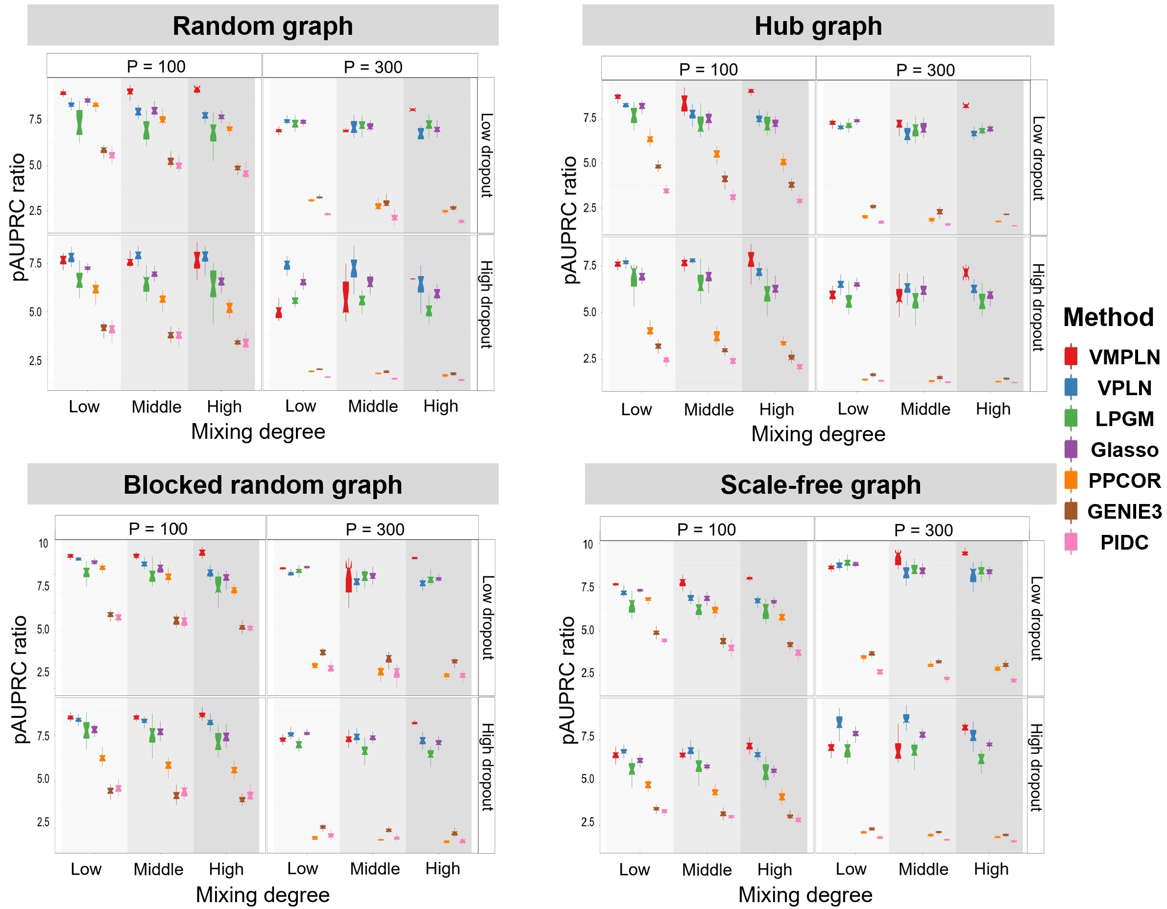
The available methods often report network estimates with very different densities. Dense network predictions usually have a high sensitivity and a low specificity, but sparse network predictions have a low sensitivity and a high specificity. In order to make dense and sparse network predictions comparable, we adopt one criteria used in a previous benchmark work on network estimation methods (Pratapa et al., 2020), called the pAUPRC ratio, to evaluate the algorithms. Briefly, given a network estimation by an algorithm, we calculate its area under the partial precision-recall curve (called pAUPRC) by applying varying thresholds to the edge scores given by the algorithm (appendix Section B.2). The pAUPRC ratio is defined as the ratio between the pAUPRC and the expected pAUPRC of the random network prediction of the same density.

We first compare the algorithms using their default parameters or default ways of selecting tuning parameters (appendix Section B.2). Figure 2 show the boxplots of pAUPRC ratios of different algorithms. Overall, VMPLN is the best-performing algorithm in terms of the pAUPCR ratio. The advantage of VMPLN is more pronounced when the populations have a higher mixing level, suggesting that compared with the two-step procedure, the joint analysis of network inference and clustering can help to improve the network inference.

Refer to caption
Figure 3: The pAUPRC ratios for four graphs. The edge score cutoffs or the tuning parameters are selected such that the network density is 20%.

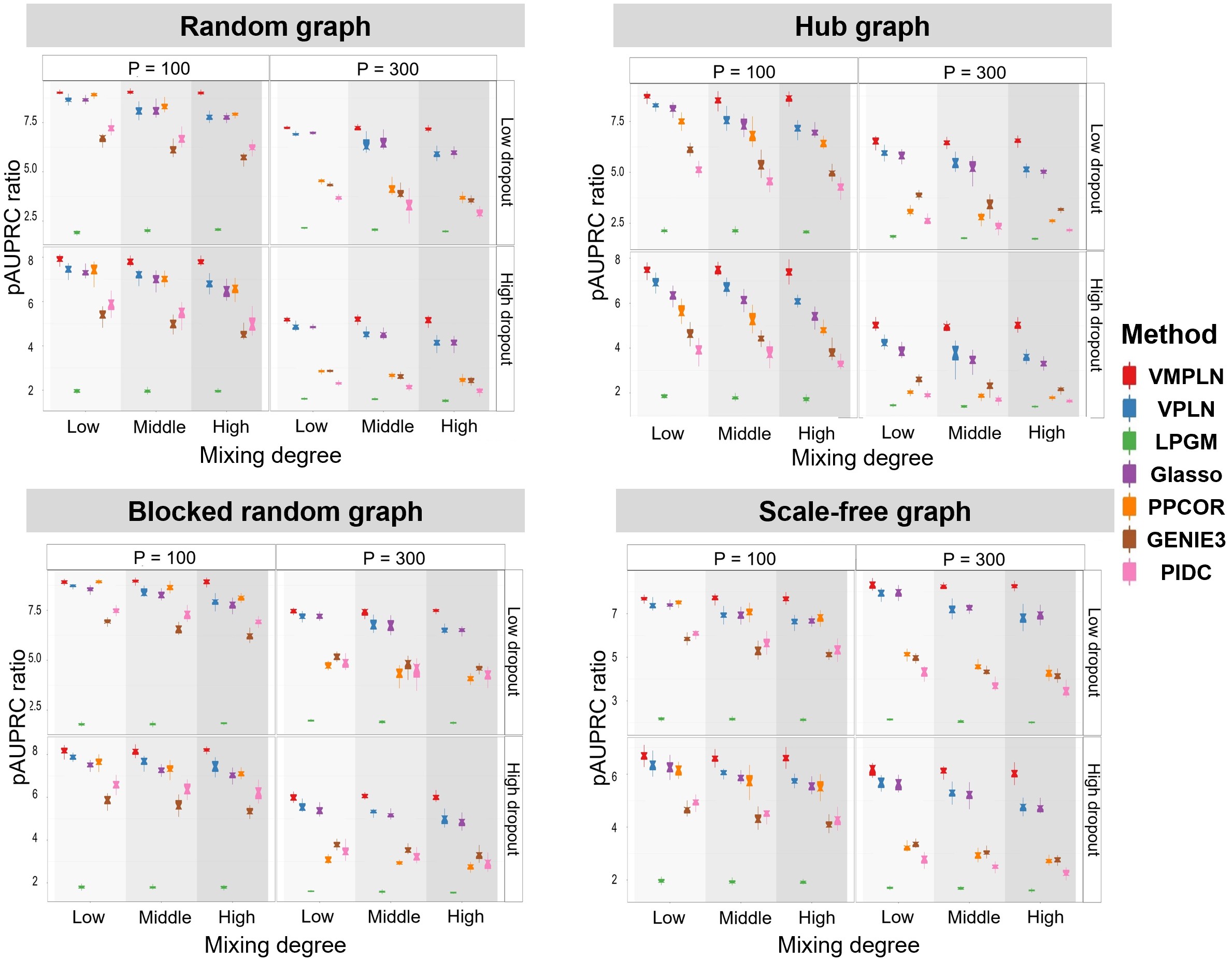
Tuning parameter selection methods can have a large impact on the network estimates. To eliminate this influence, we tune the parameters such that the estimated network from different algorithms having 20% nonzero edges (2 $\times$ the density of the true network) (appendix Section B.2), and compare their pAUPRC ratios (Figure 3). Similarly, VMPLN has the best-performance in most scenarios, especially in the cases with high mixing levels. For example, in the simulation of the hub graph with $p=100$ and low-dropout, VMPLN has mean AUPRC ratios $8.63$ and $8.72$ in the high and low mixing scenarios, respectively, about $21\%$ and $5\%$ larger than the AUPRC ratios ($7.12$ and $8.26$) of VPLN under the same scenarios. All algorithms tend to have decreased performances in higher dimensions or with high dropout rates and VMPLN consistently has better performances in these more difficult settings.

5 Real Data Analysis

Refer to caption
Figure 4: The performance of the netwok inference algorithms in two evaluation scRNA-seq datasets. The colors represent the scaled values of these metrics within each cell type and the actual values are marked in the boxes. Black color in the boxes: random predictor performs better.

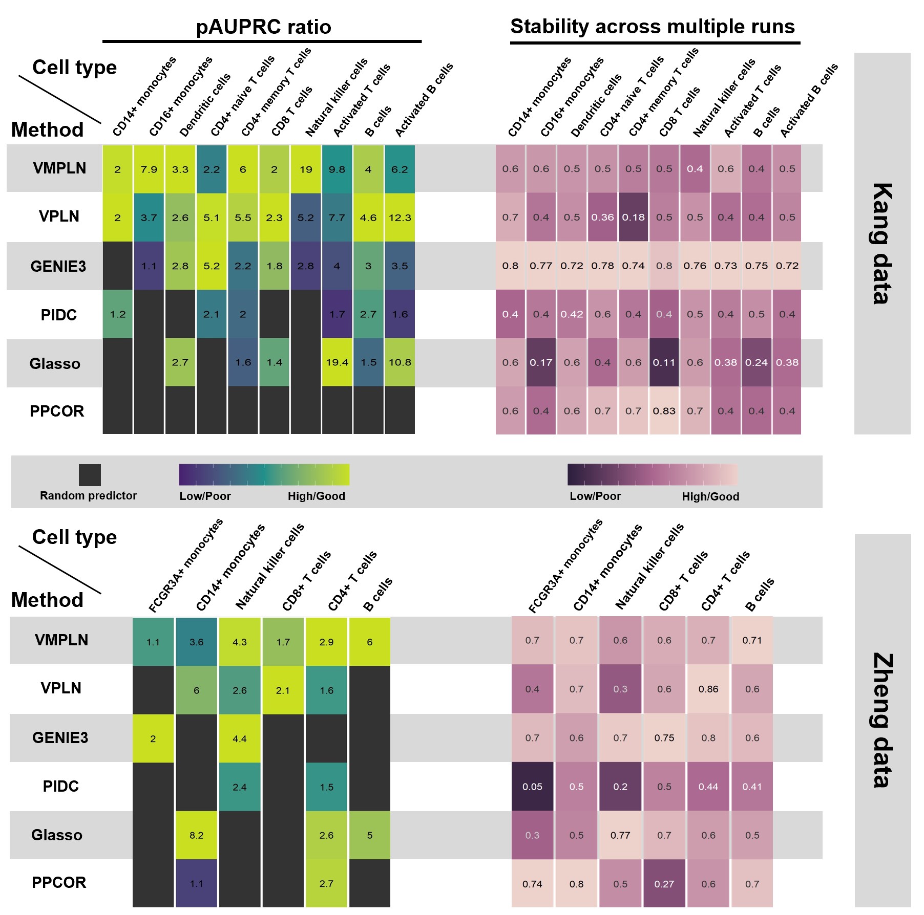
In this section, we first evaluate the performance of VMPLN and compare with other methods using two real scRNA-seq datasets for gene regulatory network inference. Then, we demonstrate an application of VMPLN to a large scRNA-seq dataset from patients infected with SARS-CoV-2. The two evaluation datasets are scRNA-seq data profiled by Kang et al. (2018) (Kang data, 7217 cells from 10 cell types) and Zheng et al. (2017) (Zheng data, 5962 cells from 6 cell types), respectively. Both datasets consist of two batches. We use one of the two batches and public gene regulatory network databases to construct silver standards (appendix Section C.1 - C.2), and test different algorithms using another batches. Regulatory relationships are inferred for the top 500 highly variable genes given by Seurat (Stuart et al., 2019) and evaluated by comparing with the silver standards.

We compare the algorithms at the same network density ($5\%$) in terms of the pAUPRC ratio and the stability (Figure 4). The pAUPRC ratios are calculated by comparing with the silver standard. The stability is defined as the median of pairwise Jaccard indexes between the networks estimated from 100 random down-sampled ($90\%$) datasets. VMPLN has the highest pAUPRC ratios in most cases and is the only method that consistently performs better than the random predictor. The stability of VMPLN is also reasonable and roughly similar to GENIE3, which is expected because GENIE3 uses data perturbation for network estimation and should have good stability.

Refer to caption
Figure 5: The gene regulatory network analysis of the SARS-CoV-2 data. (a) The inferred gene regulatory networks of Group4 macrophages in severe and moderate patients. The size of the node represents the weighted node degree. (b) Gene ontology enrichment analysis of Transcription factors’ target genes. Transcription factors are selected as those with a large weighted degree differences ($>0.2$) between severe and moderate patients. Activation and Inhibition mean that the regulatory relationships are positive and negative, respectively. Left panel: p-values of gene ontology terms. Right panel: differences of number of genes in the gene ontology terms between severe and moderate patients.

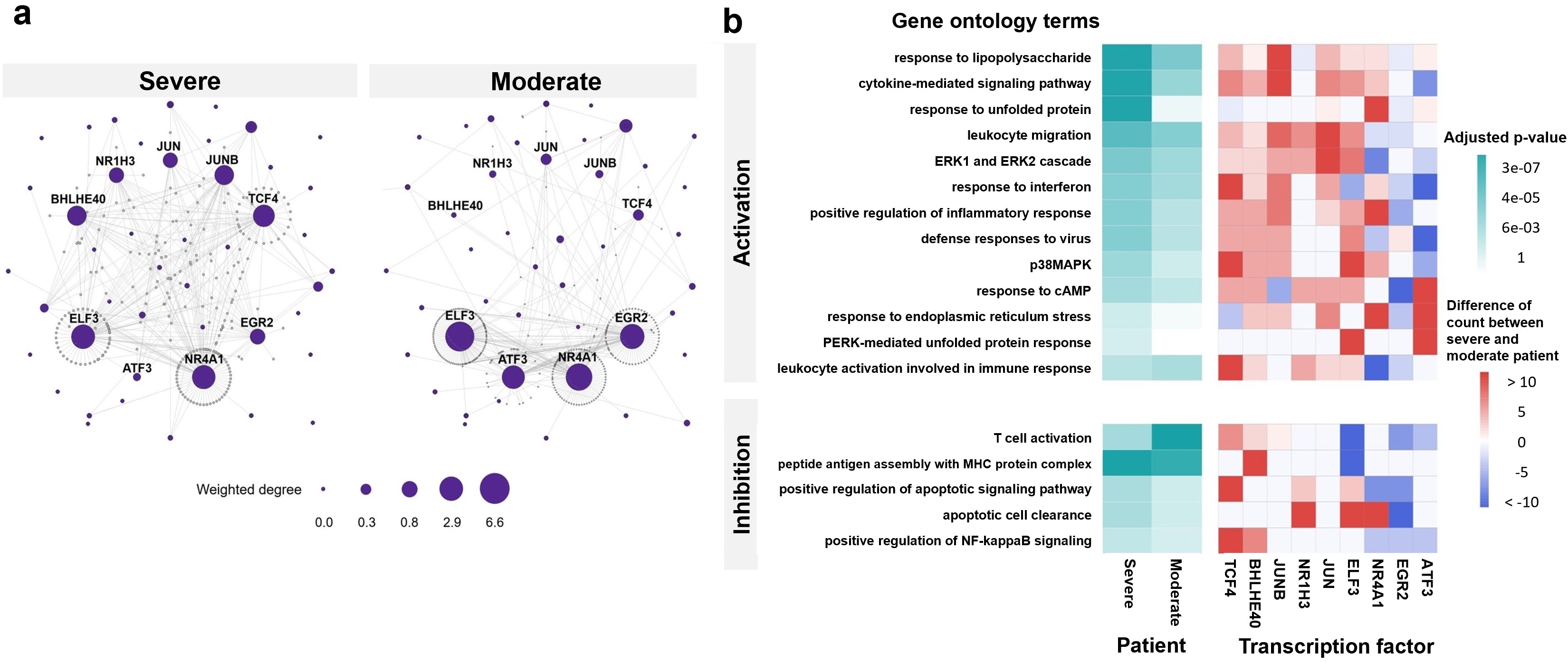
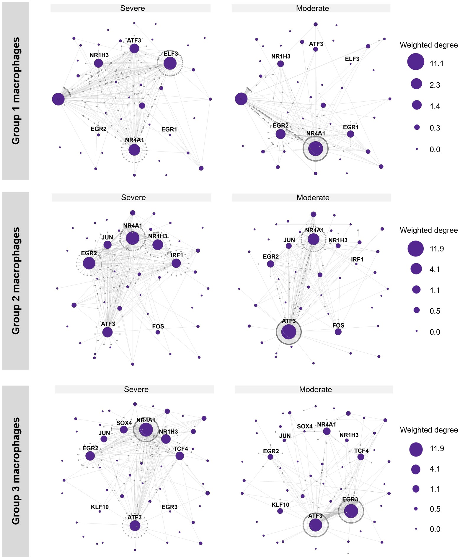
We then apply VMPLN to a SARS-CoV-2 data dataset consisting of 29,980 bronchoalveolar lavage fluid macrophage cells from 8 patients, including 2 patients with SARS-CoV-2 infection and 6 patients with severe infection. Liao et al. (2020) clustered the macrophages to four clusters including two classic M1-like macrophage groups (Group1 and Group2), the alternative M2-like macrophages (Group3) and the alveolar macrophages (Group4). The gene regulatory network of the top 1000 highly variable genes are inferred using VMPLN (Figure 5 a; appendix Section C.3 and Figure 6). We focus on the alveolar macrophages, since unlike other macrophage groups, the proportion of the alveolar macrophages tends to be smaller in patients with severe infection (Liao et al., 2020).

A number of transcription factors exhibit a large weighted degree (weighted by absolute partial correlations) difference between the gene regulatory networks in the moderate and severe patients. Gene oncology enrichment analysis of their target genes (Figure 5 b) shows that, as expected, many of target genes are involved in immune responses such as leukocyte migration and regulation of T cell activation. Interestingly, we observe that a number of gene ontology terms are only enriched in severe patients such as response to unfolded protein and response (UPR) to endoplasmic reticulum (ER) stress, mainly due to the activation of target genes of NR4A1 (Figure 5 b). The UPR and ER stress processes are frequently activated in cells infected by viruses (Janssens et al., 2014) including coronavirus (Chan et al., 2006), indicating that alveolar macrophages might be infected by SARS-CoV-2. In fact, a recent study showed that macrophages can be infected by SARS-CoV-2 and the infected macrophages activate T-cells to promote alveolitis in severe patients (Grant et al., 2021). In light of these findings, we reason that NR4A1 might play an important role in regulating cellular responses to SARS-CoV-2 infection.

6 Discussion

In this paper, we develop a regulatory network inference method called VMPLN for count data from mixed populations. Instead of using the two-step procedure for network inference, VMPLN performs clustering and network inference simultaneously, thus are better suitable for applications such as scRNA-seq studies. Since the Poisson log-normal model does not have a finite moment-generating function, common techniques for proving mixture models’ identifiability and positive-definiteness of the Fisher information matrix do not work for the mixture Poisson log-normal model. We instead use all moments to prove these basic properties of mixture models. The techniques used here may also be useful for other mixture models.


Acknowledgments and Disclosure of Funding

This work was supported by the National Key Basic Research Project of China, the National Natural Science Foundation of China, and Sino-Russian Mathematics Center.

Appendix A Appendix: Technical proofs.

A.1 Notation

For notational simplicity, we do not distinguish different lower (upper) bounds in Condition 1-3, and always use $m$ to denote the lower bound and $M$ to denote the upper bound. We always assume $M>0$. When $m$ is the lower bound for eigenvalues of precision matrices, we always assume $m>0$. We define two vectorization operators, ${\rm vech}$ and ${\rm vech_{2}}$. For a symmetric matrix $A\in\mathbb{R}^{p\times p}=[a_{ij}]$, ${\rm vech}(A)$ is defined as

$${\rm vech}(A)=(a_{11},a_{12},a_{13},\ldots,a_{1p},a_{22},a_{23},\ldots,a_{2p},\ldots,a_{(p-1)(p-1)},a_{(p-1)p},a_{pp})^{\rm T},$$

and ${\rm vech_{2}}(A)$ is

$${\rm vech_{2}}(A)=(a_{11},2a_{12},2a_{13},\ldots,2a_{1p},a_{22},2a_{23},\ldots,2a_{2p},\ldots,a_{(p-1)(p-1)},2a_{(p-1)p},a_{pp})^{\rm T}.$$

Observe that ${\rm vech}$ and ${\rm vech_{2}}$ only differ at off-diagonal elements. Define ${\nu}=(\nu_{1}^{\rm T},\ldots,\nu_{g}^{\rm T},\ldots,\nu_{G}^{\rm T})^{\rm T},$ where $\nu_{g}={\rm vech}(\Theta_{g})$. We assume the true parameter $\nu^{*}$ is an interior point of $\mathcal{D}$. For the Poisson log-normal model, we can write the log-likelihood as follows,

$$\log\,p(y,\l;\Theta,\mu)=\sum_{i=1}^{n}\log\int f(x;\Theta,\mu)p(y_{i}\mid x,l_{i})dx+\sum_{i=1}^{n}\log\left\{p(l_{i})\right\},$$

where $f(x;\Theta,\mu)$ is the probability density function of ${\rm N}(\Theta,\mu)$. Observe that $\sum_{i=1}^{n}\log\left\{p(l_{i})\right\}$ does not depend on $\Theta$. We only need to consider the conditional distribution $p(y_{i}\mid l_{i};\Theta,\mu_{g})$. Since $p(l)$ is independent of the unknown parameters and has a bounded support, it can be seen from the following section that the scaling factor $l$ does not have essential influence on the proof. For brevity, we assume that the scaling factor is the constant $1$ in the proof.

In the following sections, we always use $p(y;\Theta,\mu)$ and $p\left(y;\nu,\{\mu_{g}\}_{g=1}^{G}\right)$ to represent the density of the Poisson log-normal distribution ${\rm PLN}\left(\Theta,\mu\right)$ and the density of the mixture Poisson log-normal distribution MPLN $\left(\nu,\{\mu_{g}\}_{g=1}^{G}\right)$, respectively. Given a single sample $i$, we write the log-likelihood function of the Poisson log-normal model at $y_{i}$ as

$\displaystyle\ell(\Theta,y_{i})$ $\displaystyle=\log\left\{p(y_{i};\Theta,\mu)\right\}=2^{-1}\log\det(\Theta)$
$\displaystyle+\log\int\det(\Theta)^{1/2}\exp\left\{-2^{-1}(x-\mu)^{\rm T}\Theta(x-\mu)\right\}{h(y_{i},x)}dx+C(y_{i}),$

where

$$h(y_{i},x)=\prod_{j=1}^{p}\exp(x_{j}y_{ij})\exp\left\{-\exp(x_{j})\right\}$$ (8)

and $C(y_{i})=\sum_{j=1}^{p}\log y_{ij}!-2^{-1}p\log(2\pi)$. In the following sections, we always write $h(y,x)=\prod_{j=1}^{p}\exp(x_{j}y_{j})\exp\left\{-\exp(x_{j})\right\}$. Also, we define $\ell_{n}(\Theta)=\sum_{i=1}^{n}\ell(\Theta,y_{i})$ as the log-likelihood in the Poisson log-normal model. For the mixture Poisson log-normal model, its log-likelihood function at $y_{i}$ is

$\displaystyle\ell(\nu,y_{i})$ $\displaystyle=\log\left\{\sum_{g=1}^{G}\pi_{g}p(y_{i};\Theta_{g},\mu_{g})\right\}$
$\displaystyle=\log\left[\sum_{g=1}^{G}\pi_{g}\int\det\left(\Theta_{g}\right)^{1/2}\exp\left\{-2^{-1}(x-\mu_{g})^{\rm T}\Theta_{g}(x-\mu_{g})\right\}{h(y_{i},x)}dx\right]+C(y_{i}),$

where $C(y_{i})=\sum_{j=1}^{p}\log y_{j}!-2^{-1}p\log(2\pi)$. The log-likelihood of the mixture Poisson log-normal model is ${\ell}_{n}(\nu)=\sum_{i=1}^{n}\ell(\nu,y_{i}).$ If we define

$$L_{g}(\nu_{g},y)=\int\det(\Theta_{g})^{1/2}\exp\left\{-2^{-1}(x-\mu_{g})^{\rm T}\Theta_{g}(x-\mu_{g})\right\}{h(y,x)}dx,$$

and $L_{M}(\nu,y)=\sum_{g=1}^{G}\pi_{g}L_{g}(\nu_{g},y)$, then ${\ell}(\nu,y_{i})=\log\left\{L_{M}(\nu,y_{i})\right\}+C(y_{i})$. Observe that the function $L_{g}(\nu_{g},y)$ is proportional to the density $p(y;\Theta_{g},\mu_{g})$. Let $\mathcal{L}_{n}(\nu)=-n^{-1}\ell_{n}(\nu)$. The optimization problem (3) in the main manuscript can be written as

$$\hat{\nu}_{n}\in\operatorname*{\arg\min}_{\nu\in{\mathcal{D}}}\left\{\mathcal{L}_{n}(\nu)+{\lambda_{n}}\mathcal{R}(\nu)\right\},$$ (9)

where $\mathcal{R}(\nu)=\sum_{g=1}^{G}||\Theta_{g}||_{1,\rm off}.$

For the Poisson log-normal model, denote the derivative (the score function) and the Hessian matrix of its log-likelihood as

$$\mathcal{S}(\Theta,y)=\frac{\partial\ell(\Theta,y)}{\partial{\rm vech}(\Theta)},\quad H(\Theta,y)=\frac{\partial^{2}\ell(\Theta,y)}{\partial{\rm vech}(\Theta)\partial{\rm vech}(\Theta)^{\rm T}}.$$

For the mixture Poisson log-normal model, we can similarly define its score function $\mathcal{S}^{M}(\nu,y)$, its Hessian matrix ${F}(\nu,y)$, and its Fisher information matrix $\Gamma^{*}=\Gamma(\nu^{*})$.

$${D}(\nu)={E}_{\nu^{*}}\left\{{F}(\nu,y)\right\}.$$ (10)

Observe that ${D}(\nu^{*})=-\Gamma(\nu^{*})$.

Finally, we denote $\mathbb{N}^{p}$ as the set of all $p$-dimensional non-negative integer vectors. For a vector ${a}=(a_{1},\ldots,a_{p})$, we denote $||{a}||_{2}=\sqrt{\sum_{j=1}^{p}a_{j}^{2}}$ as its $L_{2}$-norm and $||{a}||_{\infty}=\max_{j}|a_{j}|$ as its $L_{\infty}$-norm. For a matrix ${A}$, we denote $||{A}||_{2}$ as its largest singular value of ${A}$ and $||{A}||_{1,\infty}$ as its maximum absolute row sum of ${A}$. Given ${\Theta}$ and ${\mu}$, we define an operator $\mathcal{T}$ that maps functions in $x$ to functions in $y$, $\mathcal{T}(f)=\int\exp\left\{-2^{-1}({x}-{\mu})^{\rm T}{\Theta}({x}-{\mu})\right\}f({x})h({y},{x})d{x}.$ We use $\mathbb{I}({x})\equiv 1$ as the constant function taking value 1.

A.2 Some Lemmas

Lemma 4

Let ${y}\sim{\rm PLN}({\Theta},{\mu})$. For any $n,y\in\mathbb{N}$, we define $\phi(y,n)=\prod_{i=1}^{n}(y-i+1)$ if $n>0$ and $\phi(y,n)=1$ if $n=0$. Then, for ${N}=(n_{1},\dots,n_{p})^{\rm T}$, we have ${E}\left(\prod_{j=1}^{p}\phi({n_{j}},y_{j})\right)=\exp\left({{N}}^{\rm T}{\mu}+{{N}}^{\rm T}{\Theta}^{-1}{N}/2\right).$

Lemma 5 (1-dimensional dominating function)

Suppose $\theta\in[m,M]$ ($m,M>0$), and $|\mu|\leq M$. Let

$$f^{1}(y,\theta,\mu)={\int\exp\left\{-2^{-1}\theta(x-\mu)^{2}\right\}\exp\left\{-\exp(x)\right\}\exp(xy)dx}.$$

Then, for any large enough positive integer $y$, we have $f^{1}(y,\theta,\mu)\geq C\exp\left\{y\log(y+1)/2\right\},$ where $C>0$ is constant depending on $m,M$.

Lemma 6 ($p$-dimensional dominating function)

Let

$$f^{p}({y},{\Theta},{\mu})=\frac{\mathcal{T}\left\{(x_{1}-\mu_{1})^{4}\right\}}{\mathcal{T}(\mathbb{I})},$$ (11)

where ${y}=(y_{1},\dots,y_{p})\in\mathbb{N}^{p}$. Assuming ${y}\sim{\rm PLN}({\Theta}^{*},{\mu})$, under Condition 1-3, there exists a polynomial function $g({y})=\left(4||{y}||_{2}/m\right)^{4}+C_{p}$ with a constant $C_{p}$ only depending on $p,m$ and $M$, such that ${E}_{{\Theta}^{*}}(g({y}))<\infty$ and $|f^{p}({y},{\Theta},{\mu})|\leq g({y})$ for any ${\Theta},{\mu}$ satisfying Condition 1-3.

Remark 7

Applying the same proof as in Lemma 6, the polynomial $(x_{1}-\mu_{1})^{4}$ can be replaced by any polynomial with respect to ${x}$, e.g. $(x_{i}-\mu_{i})^{2}(x_{j}-\mu_{j})^{2}$ and $(x_{i}-\mu_{i})(x_{j}-\mu_{j})(x_{k}-\mu_{k})^{2}$. Further, for any two polynomial functions ${\psi}_{1}({x}),{\psi}_{2}({x})$ and $f^{p}({y},{\Theta},{\mu})={\mathcal{T}\left\{{\psi}_{1}({x})\right\}\mathcal{T}\left\{{\psi}_{2}({x})\right\}}/{\mathcal{T}^{2}(\mathbb{I})},$ there exists a polynomial function $g({y})$ with ${E}_{\Theta^{*}}(g({y}))<\infty$ such that $|f^{p}({y},{\Theta},{\mu})|\leq g({y})$ for any ${\Theta},{\mu}$ satisfying Condition 1-3.

Proof [of Lemma 4] By the property of conditional expectation, we have ${E}\left(\prod_{j=1}^{p}\phi({n_{j}},y_{j})\right)={E}_{{x}}{E}_{{y}}\left(\prod_{j=1}^{p}\phi({n_{j}},y_{j})\mid{x}\right).$ From the moments of the Poisson distribution, we have

$${E}_{{y}}\left(\prod_{j=1}^{p}\phi({n_{j}},y_{j})\mid{x}\right)=\prod_{j=1}^{p}\exp(n_{j}x_{j}).$$

Further, since ${x}\sim{\rm N}({\mu},{\Theta}^{-1})$, we have

$${E}_{{x}}\left(\prod_{j=1}^{p}\exp(n_{j}x_{j})\right)={E}_{{x}}\left\{\exp({N}^{\rm T}{x})\right\}=\exp\left({N}^{\rm T}{\mu}+{N}^{\rm T}{\Theta}^{-1}{N}/2\right),$$

and the conclusion follows.  

Proof [of Lemma 5] Since for any $y\in\mathbb{N}$, $f^{1}(y,\theta,\mu)>0$, we only need to consider $y$ large enough. Let $g(x,y)=\exp\left\{-2^{-1}\theta(x-\mu)^{2}\right\}\exp\left\{-\exp(x)\right\}\exp(xy).$ Clearly, we have, for $y$ large enough, $\int g(x,y)dx\geq\int_{\log(y)-1}^{\log(y)}g(x,y)dx.$ Let $t=x-\log(y)$, then

$\displaystyle\quad\int_{\log(y)-1}^{\log(y)}g(x,y)dx$
$\displaystyle=\exp\left\{y\log(y)\right\}\int_{-1}^{0}\exp\left[-2^{-1}\theta\left\{\log(y)+t-\mu\right\}^{2}\right]\exp\left[-\exp\left\{\log(y)+t\right\}\right]\exp(yt)dt$
$\displaystyle\geq\exp\left\{y\log(y)\right\}\min_{t\in[-1,0]}\left(\exp\left[-2^{-1}\theta\left\{\log(y)-t-\mu\right\}^{2}\right]\right)\int_{-1}^{0}\exp\left[y\left\{t-\exp(t)\right\}\right]dt.$
$\displaystyle\geq\exp\left\{y\log(y)-y\right\}\min_{t\in[-1,0]}\left(\exp\left[-2^{-1}\theta\left\{\log(y)-t-\mu\right\}^{2}\right]\right)\int_{-1}^{0}\exp(-t^{2}/2)dt/\sqrt{y}.$
$\displaystyle\geq\exp\left\{y\log(y)-y\right\}C_{2}\exp\left\{-C_{3}\log^{2}(y)+C_{4}\log(y)\right\}/\sqrt{y},$ (12)

where $C_{2}$, $C_{3}$ and $C_{4}$ are three constants only depending on $m,M$. Since the leading order of (A.2) is $\exp\left\{y\log(y)-y\right\}$ , when $y\geq 1$, there exists a constant $C$ depending on $m,M$ such that for any large enough positive integer $y$, we have $f^{1}(y,\theta,\mu)\geq C\exp\left\{y\log(y+1)/2\right\},$ which proves the conclusions.  

Proof [of Lemma 6] Similarly, we only need to consider $||{y}||_{2}$ large enough. The proof consists of the following three steps.

Step 1. We first give a lower bound for the denominator of (11). Observe that

$$\exp\left\{-2^{-1}({x}-{\mu})^{\rm T}{\Theta}({x}-{\mu})\right\}\geq\exp\left\{-2^{-1}M({x}-{\mu})^{\rm T}({x}-{\mu})\right\}.$$

We have

$\displaystyle\quad\int\exp\left\{-2^{-1}({x}-{\mu})^{\rm T}{\Theta}({x}-{\mu})\right\}h({y},{x})d{x}\geq\int\exp\left\{-2^{-1}M({x}-{\mu})^{\rm T}({x}-{\mu})\right\}h({y},{x})d{x}$
$\displaystyle=\prod_{j=1}^{p}\int\exp\left\{-2^{-1}M(x_{j}-\mu_{j})^{2}\right\}\exp\left\{-\exp(x_{j})\right\}\exp(x_{j}y_{j})dx_{j}.$

By Lemma 5, we have, for any fixed $j$, $\int\exp\left\{-2^{-1}M(x_{j}-\mu_{j})^{2}\right\}\exp\left\{-\exp(x_{j})\right\}\exp(x_{j}y_{j})dx_{j}$ is greater than $C\exp\left\{y_{j}\log(y_{j}+1)/2\right\}$. Hence, we have $\int\exp\left\{-2^{-1}({x}-{\mu})^{\rm T}{\Theta}({x}-{\mu})\right\}h({y},{x})d{x}\geq C^{p}\exp\left\{\sum_{j}y_{j}\log(y_{j}+1)/2\right\}.$

Step 2. When $||{x}-{\mu}||_{2}\leq A({y})=4||{y}||_{2}/m$, we have $(x_{1}-\mu_{1})^{4}\leq||{x}-{\mu}||_{2}^{4}\leq A^{4}({y})$, where $x_{1}$ is the first element of ${x}$. Then, we have

$$\frac{\int_{||{x}-{\mu}||_{2}\leq A}\exp\left\{-2^{-1}({x}-{\mu})^{\rm T}{\Theta}({x}-{\mu})\right\}(x_{1}-\mu_{1})^{4}h({y},{x})d{x}}{\int\exp\left\{-2^{-1}({x}-{\mu})^{\rm T}{\Theta}({x}-{\mu})\right\}h({y},{x})d{x}}\leq A^{4}({y}).$$

Since $A^{4}({y})$ is a polynomial function of ${y}$, we have ${E}_{{\Theta}^{*}}(A^{4}({y}))<\infty.$

Step 3. When $||{x}-{\mu}||_{2}>A({y})$, we have

$\displaystyle\quad\int_{||{x}-{\mu}||_{2}>A({y})}\exp\left\{-2^{-1}({x}-{\mu})^{\rm T}{\Theta}({x}-{\mu})\right\}(x_{1}-\mu_{1})^{4}h({y},{x})d{x}$
$\displaystyle\leq\int_{||{x}-{\mu}||_{2}>A({y})}\exp\left\{-2^{-1}({x}-{\mu})^{\rm T}{\Theta}({x}-{\mu})\right\}(x_{1}-\mu_{1})^{4}\exp\left(\sum_{j=1}^{p}x_{j}{y_{j}}\right)d{x}$
$\displaystyle=\prod_{j=1}^{p}\exp(\mu_{j}{y_{j}})\int_{||{{u}}||_{2}>A({y})}\exp\left(-2^{-1}{{u}}^{\rm T}{\Theta}{{u}}\right)u_{1}^{4}\prod_{j=1}^{p}\exp(u_{j}{y_{j}})d{{u}}\quad({{u}}={x}-{\mu})$
$\displaystyle\leq\prod_{j=1}^{p}\exp(\mu_{j}{y_{j}})\int_{||{{u}}||_{2}>A({y})}\exp\left(-2^{-1}m||{{u}}||_{2}^{2}\right)||{{u}}||_{2}^{4}\exp(||{{u}}||_{2}||{y}||_{2})d{{u}},$

where the last inequality is by Cauchy’s inequality. Observe that the area of the $p$-dimensional sphere of radius $r$ is $M_{p}r^{p-1}$ with $M_{p}$ being a constant only depending on $p$. Let $r=||{{u}}||_{2}$. By the polar decomposition, the $p$-dimensional integral can be rewritten as

$\displaystyle\quad\int_{||{{u}}||_{2}>A({y})}\exp\left(-2^{-1}m||{{u}}||_{2}^{2}\right)||{{u}}||_{2}^{4}\exp\left(||{{u}}||_{2}||{y}||_{2}\right)d{{u}}$
$\displaystyle=\int_{r>A({y})}\exp\left\{-2^{-1}r\left(mr-2||{y}||_{2}\right)\right\}M_{p}r^{p+3}dr$
$\displaystyle\leq\int_{r>A({y})}\exp(-r||{y}||_{2})M_{p}r^{p+3}dr\quad\left(r>4\frac{||{y}||_{2}}{m}\right)$
$\displaystyle\leq\int_{r>A({y})}\exp(-r)M_{p}r^{p+3}dr=C^{\prime}_{p},$

where $C^{\prime}_{p}$ is a constant only depending on $p$. Then, under Condition 1-3, we have

$$\frac{\int_{||{x}-{\mu}||_{2}\leq A}\exp\left\{-2^{-1}({x}-{\mu})^{\rm T}{\Theta}({x}-{\mu})\right\}(x_{1}-\mu_{1})^{4}h({y},{x})d{x}}{\int\exp\left\{-2^{-1}({x}-{\mu})^{\rm T}{\Theta}({x}-{\mu})\right\}h({y},{x})d{x}}\leq\frac{\prod_{j=1}^{p}\exp(\mu_{j}{y_{j}})C^{\prime}_{p}}{\exp\left\{\sum_{j}y_{j}\log(y_{j}+1)/2\right\}}\leq C_{p}$$

where $C_{p}$ is a constant depending on $p,m$ and $M$.

Finally, combining the results in Step 2 and 3, we get the dominating function $g({y})=\left(4||{y}||_{2}/m\right)^{4}+C_{p}$ which is a polynomial. By Lemma 4, we have ${E}_{{\Theta}^{*}}(g({y}))<\infty$.  

A.3 Proof of Theorem 1, Part I

To prove the the first conclusion of Theorem 1, we introduce the following definition and give two lemmas.

Definition 8 (Good vector)

We call a vector ${\xi}=(\xi_{1},\dots,\xi_{G})^{\rm T}\in\mathbb{R}^{G}$ as a good vector if one $\xi_{g}$ only appears once in ${\xi}$, i.e. $\xi_{g^{\prime}}\neq\xi_{g}$ for all $g^{\prime}\neq g$. We call the index $g$ as a good index with respect to ${\xi}$.

Lemma 9

Let ${\xi}=(\xi_{1},\dots,\xi_{G})^{\rm T}$ be a good vector with a good index $s$, ${\sigma}=(\sigma_{1},\dots,\sigma_{G})^{\rm T}$ satisfy $\sigma_{g}>0$ for $g=1,\dots,G$ and ${\alpha}=(\alpha_{1},\dots,\alpha_{G})^{\rm T}$. If for any $z\in\mathbb{N}$, $\sum_{g=1}^{G}\alpha_{g}\exp(\xi_{g}z+\sigma_{g}z^{2}/2)=0,$ then $\alpha_{s}=0$.

Lemma 10

For any $n>0$, let $\mathcal{M}_{i}\subset\mathbb{R}^{p},i=1,\dots,n$ be $n$ linear proper subspaces. Then, there exists a non-negative integer vector ${\gamma}$ such that ${\gamma}\not\in\bigcup_{i=1}^{n}\mathcal{M}_{i}$.

Proposition 11

$p\left({y};{\Theta}_{1},{\mu}_{1}\right),\dots,p\left({y};{\Theta}_{G},{\mu}_{G}\right)$ are linearly independent for ${\mu}_{g}$ ($g=1,\dots,G$) that are bounded and different from each other.

Proof [of Theorem 1 part I] By Yakowitz and Spragins (1968), under Condition 1-3, the identifiability of the mixture Poisson log-normal model is equivalent to the linear independence of the Poisson log-normal components. Thus, we aim to prove Proposition 11. We prove this by mathematical induction.

The independence for $G=1$ is trivial. Now we assume that Proposition 11 holds for $G-1$. For any ${\mu}_{1},\dots,{\mu}_{G}$ that are bounded and different from each other, if we can prove that there exists ${\alpha}=(\alpha_{1},\dots,\alpha_{G})^{\rm T}$ and an index $s\in\{1,\dots,G\}$ such that $\sum_{g=1}^{G}\alpha_{g}p\left({y};{\Theta}_{g},{\mu}_{g}\right)=0\mbox{ and }\alpha_{s}=0,$ then by induction, we have ${\alpha}=0$ and hence $p({y};{\Theta}_{g},{\mu}_{g})$ ($g=1,\dots,G$) are linearly independent. So our goal is to prove that if $\sum_{g=1}^{G}\alpha_{g}p({y};{\Theta}_{g},{\mu}_{g})=0$, then we can always find an index $s$ such that $\alpha_{s}=0$.

Let ${N}=(n_{1},\dots,n_{p})^{\rm T}$ be any non-negative integer vector. Then, for any positive integer $z$, by Lemma 4, there exists a polynomial function $p_{z}({y})=\prod_{j=1}^{p}\phi(zn_{j},y_{j}),z\in\mathbb{N}$ such that

$$\sum_{g=1}^{G}\alpha_{g}{E}_{g}\left\{p_{z}({y})\right\}=0\mbox{ and }{E}_{g}\left\{p_{z}({y})\right\}=\exp\left(zN^{\rm T}{\mu}_{g}+z^{2}{N}^{\rm T}{\Theta}^{-1}_{g}{N}/2\right),$$

where ${E}_{g}$ represents taking expectation with respect to ${\rm PLN}\left({\Theta}_{g},{\mu}_{g}\right)$. Let

$${\xi}=\left(N^{\rm T}{\mu}_{1},\dots,N^{\rm T}{\mu}_{G}\right)\ \mbox{and}\ {\sigma}=\left({N}^{\rm T}{\Theta}^{-1}_{1}N/2,\dots,{N}^{\rm T}{\Theta}^{-1}_{G}{N}/2\right).$$

By Lemma 9, if there exists an $N$ such that ${\xi}$ is a good vector with good index $s$, then $\alpha_{s}=0$ and we complete the proof. If, on the other hand, ${\xi}=\left(N^{\rm T}{\mu}_{1},\dots,N^{\rm T}{\mu}_{G}\right)$ is not a good vector for any non-negative integer vector $N$. Therefore, for any $N$, there exists $s\neq 1$ such that $N^{\rm T}{\mu}_{1}=N^{\rm T}{\mu}_{s}$. Thus, $N$ is the solution to the linear equation ${x}^{\rm T}({\mu}_{1}-{\mu}_{s})=0$. We define $\mathcal{M}_{g}$ as the linear space consisting of solutions to the linear equation ${x}^{\rm T}\left({\mu}_{1}-{\mu}_{g}\right)=0$ ($g\neq 1$) and $\mathcal{M}=\cup_{g=2}^{G}\mathcal{M}_{g}$. Thus, for any non-negative integer vector $N$, we have $N\in\mathcal{M}$. Since ${\mu}_{g}$ are different form each other, then $\dim{\mathcal{M}_{g}}=p-1$ and $\mathcal{M}_{g}$ is a proper subspace of $\mathbb{R}^{p}$. This is contradictory to Lemma 10. So there exists an $N$ such that ${\xi}=\left(N^{\rm T}{\mu}_{1},\dots,N^{\rm T}{\mu}_{G}\right)$ is a good vector and hence for any ${\mu}_{g}$ ($g=1,\dots,G$) that are different from each other, $p({y};{\Theta}_{1},{\mu}_{1}),\dots,p({y};{\Theta}_{G},{\mu}_{G})$ are linearly independent.  

Proof [of Lemma 9] Without loss of generality, we assume that $(\xi_{g},\sigma_{g})$ ($g=1,\dots,G$) are increasingly ordered (first by $\xi$ then by $\sigma$). We say that $(\xi_{g},\sigma_{g})$ and $(\xi_{s},\sigma_{s})$ are equivalent if $(\xi_{g},\sigma_{g})=(\xi_{s},\sigma_{s})$. By this equivalence relationship, $\{(\xi_{g},\sigma_{g})\}_{g=1}^{G}$ can be partitioned into $Q$ groups ($Q\geq 1$). Let $S_{q}$ be the index set of the $q$-th group. We have $\sum_{q=1}^{Q}\sum_{j\in S_{q}}\alpha_{j}\exp(\xi_{j}z+\sigma_{j}z^{2}/2)=0$ for all $z\in\mathbb{N}$. Dividing $\exp(\xi_{G}z+\sigma_{G}z^{2}/2)$ on both sides of the above equation, we get

$$\sum_{q=1}^{Q-1}\sum_{j\in S_{q}}\alpha_{j}\exp(\xi_{j}z+\sigma_{j}z^{2}/2-\xi_{G}z-\sigma_{G}z^{2}/2)+\sum_{j\in S_{Q}}\alpha_{j}=0$$ (13)

for all $z\in\mathbb{N}$. By the choice of $\sigma_{G},\xi_{G}$, the first summation of (13) converges to zero when $z$ goes to infinity. So, we have $\sum_{j\in S_{Q}}\alpha_{j}=0$. By mathematical induction, we have $\sum_{j\in S_{q}}\alpha_{j}=0$ for $q=1,\dots,Q$. Since ${\xi}$ is a good vector with a good index $s$, ($\xi_{s},\sigma_{s}$) itself forms a group, and hence $\alpha_{s}=0$.  

Proof [of Lemma 10] We prove by mathematical induction. The conclusion clearly holds for $n=1$. Now we assume that Lemma 10 holds for $n$ and we aim to prove that it also holds for $n+1$.

By induction hypothesis, we can take ${\alpha}\in\mathbb{N}^{p}\setminus\bigcup_{i=1}^{n}\mathcal{M}_{i}$. If ${\alpha}\not\in\mathcal{M}_{n+1}$, we have ${\alpha}\not\in\bigcup_{i=1}^{n+1}\mathcal{M}_{i}$, and the proof is finished. Thus, we only need to consider ${\alpha}\in\mathcal{M}_{n+1}$. Similarly, we can take ${{\beta}}\in\mathbb{N}^{p}\setminus\bigcup_{i=2}^{n+1}\mathcal{M}_{i}$ and ${{\beta}}\in\mathcal{M}_{1}$. For any $i\neq 1$, we can prove that there is at most one $k_{1}$ such that ${\alpha}+k_{1}{\beta}\in\mathcal{M}_{i}$. In fact, if there are $k_{1},k_{2}$ such that $k_{1}\neq k_{2}$ and ${\alpha}+k_{1}{{\beta}}\in\mathcal{M}_{i},{\alpha}+k_{2}{{\beta}}\in\mathcal{M}_{i}$, then ${{\beta}}\in\mathcal{M}_{i}$, which is contradictory to the fact that ${{\beta}}\in\mathbb{N}^{p}\setminus\bigcup_{i=2}^{n+1}\mathcal{M}_{i}$. Furthermore, there is no $k\in\mathbb{N}$ such that ${\alpha}+k{{\beta}}\in\mathcal{M}_{1}$. If otherwise, there exists a $k\in\mathbb{N}$ such that ${\alpha}+k{{\beta}}\in\mathcal{M}_{1}$. Then, we have ${\alpha}\in\mathcal{M}_{1}$, which is also a contradiction. So we could find at most $n$ positive integers $k$ such that ${\alpha}+k{{\beta}}\in\bigcup_{i=1}^{n+1}\mathcal{M}_{i}$. Since there are infinitely many non-negative numbers, we prove that there exists $k\in\mathbb{N}$ such that ${\alpha}+k{{\beta}}\not\in\bigcup_{i=1}^{n+1}\mathcal{M}_{i}$, and Lemma 10 is proved.  

A.4 Proof of Theorem 1, Part II

To prove this conclusion, we need to give the explicit formula for the score functions and the Fisher information matrices of the Poisson log-normal model and mixture Poisson log-normal model. The Hessian matrix ${H}\left({\Theta},{y}\right)$ of the Poisson log-normal model is a $p(p+1)/2\times p(p+1)/2$ matrix. For notational convenience, we let ${H}_{(i,j)(i^{\prime},j^{\prime})}=\partial^{2}\ell({\Theta},{y})/(\partial\Theta_{i^{\prime}j^{\prime}}\partial\Theta_{ij})$, $(i\leq j,i^{\prime}\leq j^{\prime})$ as the element at the $(2p-i+1)i/2-p+j$ row and $(2p-i^{\prime}+1)i^{\prime}/2-p+j^{\prime}$ column of the Hessian matrix. It is clear that the densities of the Poisson log-normal distribution and mixture Poisson log-normal distribution satisfy the regularity conditions in Shao (2003). Then, we can calculate the score function and the Fisher information as follows. The score function of the Poisson log-normal distribution can be written as

$\displaystyle\mathcal{S}({\Theta},{y})=$ $\displaystyle 2^{-1}{\rm vech_{2}}\left({\Theta}^{-1}\right)$
$\displaystyle-2^{-1}\frac{\int\exp\left\{-2^{-1}({x}-{\mu})^{\rm T}{\Theta}({x}-{\mu})\right\}{\rm vech_{2}}\left\{({x}-{\mu})({x}-{\mu})^{\rm T}\right\}h({y},{x})d{x}}{\int\exp\left\{-2^{-1}({x}-{\mu})^{\rm T}{\Theta}({x}-{\mu})\right\}h({y},{x})d{x}}.$

Especially, at the true parameter ${\Theta}^{*}$ , we have

$$\mathcal{S}({\Theta}^{*},{y})=2^{-1}{E}_{{x}}\left\{{\rm vech_{2}}\left({\Theta}^{*-1}-({x}-{\mu})({x}-{\mu})^{\rm T}\right)\mid{y}\right\}.$$

We use $(i,j),i\leq j$ to index $\mathcal{S}$. Using the operator $\mathcal{T}$, the element of the score function at $(2p-i+1)i/2-p+j$ can be rewritten as $\mathcal{S}_{(i,j)}\left({\Theta},{y}\right)=2^{-1}{\rm vech_{2}}\left({\Theta}^{-1}\right)_{(i,j)}-2^{-1}\frac{\mathcal{T}\left[{\rm vech_{2}}\left\{({x}-{\mu})({x}-{\mu})^{\rm T}\right\}_{(i,j)}\right]}{\mathcal{T}\left(\mathbb{I}\right)}.$ Using the operator $\mathcal{T}$, the Fisher information matrix can be written as follows. Let $\Sigma={\Theta}^{-1}.$ When $i=j,i^{\prime}=j^{\prime}$,

$\displaystyle{H}_{(i,i)(i^{\prime},i^{\prime})}\left({\Theta},{y}\right)$ $\displaystyle=-2^{-1}\Sigma_{ii^{\prime}}\Sigma_{i^{\prime}i}+\frac{1}{4}\frac{\mathcal{T}\left\{{({{x}-{\mu}})}_{i}^{2}({{x}-{\mu}})_{i^{\prime}}^{2}\right\}}{\mathcal{T}\left(\mathbb{I}\right)}$
$\displaystyle-\frac{1}{4}\frac{\mathcal{T}\left\{({{x}-{\mu}})_{i^{\prime}}^{2}\right\}\mathcal{T}\left\{{({{x}-{\mu}})}_{i}^{2}\right\}}{\mathcal{T}^{2}\left(\mathbb{I}\right)}.$

When $i\neq j,i^{\prime}=j^{\prime}$,

$\displaystyle{H}_{(i,j)(i^{\prime},i^{\prime})}\left({\Theta},{y}\right)$ $\displaystyle=-\Sigma_{ii^{\prime}}\Sigma_{i^{\prime}j}+2^{-1}\frac{\mathcal{T}\left\{{({{x}-{\mu}})}_{i}{({{x}-{\mu}})}_{j}({{x}-{\mu}})_{i^{\prime}}^{2}\right\}}{\mathcal{T}\left(\mathbb{I}\right)}$
$\displaystyle-2^{-1}\frac{\mathcal{T}\left\{({{x}-{\mu}})_{i^{\prime}}^{2}\right\}\mathcal{T}\left\{{({{x}-{\mu}})}_{i}{({{x}-{\mu}})}_{j}\right\}}{\mathcal{T}^{2}\left(\mathbb{I}\right)}.$

When $i=j,i^{\prime}\neq j^{\prime}$,

$\displaystyle{H}_{(i,i)(i^{\prime},j^{\prime})}\left({\Theta},{y}\right)$ $\displaystyle=-\Sigma_{ii^{\prime}}\Sigma_{j^{\prime}i}+2^{-1}\frac{\mathcal{T}\left\{{({{x}-{\mu}})}_{i^{\prime}}{({{x}-{\mu}})}_{j^{\prime}}({{x}-{\mu}})_{i}^{2}\right\}}{\mathcal{T}\left(\mathbb{I}\right)}$
$\displaystyle-2^{-1}\frac{\mathcal{T}\left\{({{x}-{\mu}})_{i}^{2}\right\}\mathcal{T}\left\{{({{x}-{\mu}})}_{i^{\prime}}{({{x}-{\mu}})}_{j^{\prime}}\right\}}{\mathcal{T}^{2}(\mathbb{I})}.$

When $i\neq j,i^{\prime}\neq j^{\prime}$,

$\displaystyle{H}_{(i,j)(i^{\prime},j^{\prime})}\left({\Theta},{y}\right)$ $\displaystyle=-(\Sigma_{ii^{\prime}}\Sigma_{j^{\prime}j}+\Sigma_{ij^{\prime}}\Sigma_{i^{\prime}j})+\frac{\mathcal{T}\left\{{({{x}-{\mu}})}_{i^{\prime}}{({{x}-{\mu}})}_{j^{\prime}}({{x}-{\mu}})_{i}({{x}-{\mu}})_{j}\right\}}{\mathcal{T}\left(\mathbb{I}\right)}$
$\displaystyle-\frac{\mathcal{T}\left\{({{x}-{\mu}})_{i}({{x}-{\mu}})_{j}\right\}\mathcal{T}\left\{{({{x}-{\mu}})}_{i^{\prime}}{({{x}-{\mu}})}_{j^{\prime}}\right\}}{\mathcal{T}^{2}\left(\mathbb{I}\right)}.$
Lemma 12

Assume ${y}\sim{\rm PLN}({\Theta},{\mu})$. Under Condition 1-3, there exist two polynomial functions $K_{1}({y}),K_{2}({y})$ with ${E}\left(K_{1}(y)\right)<\infty$ and ${E}\left(K_{2}(y)\right)<\infty$ such that for any $i,j,i^{\prime},j^{\prime}$, $|\mathcal{S}_{(i,j)}({\Theta},{y})|\leq K_{1}({y})$, $|{H}_{(i,i)(i^{\prime},i^{\prime})}({\Theta},{y})|\leq K_{2}({y})$.

Now we consider the score function and the Fisher information matrix of the mixture Poisson log-normal distribution. The score function of the mixture Poisson log-normal distribution can be written as

$$\mathcal{S}^{M}({\nu},{y})=L_{M}({\nu},{y})^{-1}\left({\pi_{1}\frac{\partial L_{1}({\nu}_{1},{y})}{\partial{\nu}_{1}}},\ldots,{\pi_{G}\frac{\partial L_{G}({\nu}_{G},{y})}{\partial{\nu}_{G}}}\right)=\left\{\mathcal{S}^{M}_{1}({\nu},{y}),\dots,\mathcal{S}^{M}_{G}({\nu},{y})\right\}.$$

Similarly, we use $(g,i,j),i\leq j$ to index $\mathcal{S}^{M}$. Recall that ${\nu}_{g}={\rm vech}({\Theta}_{g})$. We use $(g,i,j),(g^{\prime},i^{\prime},j^{\prime}),i\leq j,i^{\prime}\leq j^{\prime}$ to index the element at the $(g-1)p(p+1)/2+(2p-i+1)i/2-p+j$ row and $(g^{\prime}-1)p(p+1)/2+(2p-i^{\prime}+1)i^{\prime}/2-p+j^{\prime}$ column of $F({\nu},{y})$, respectively.

When $g=g^{\prime}$

$\displaystyle{F}_{(g,i,j,g,i^{\prime},j^{\prime})}({\nu},{y})$ $\displaystyle=\frac{\partial}{{\partial{\Theta}_{g,i^{\prime}j^{\prime}}}}\mathcal{S}^{M}_{(g,i,j)}({\nu},{y})$
$\displaystyle=\frac{\pi_{g}L_{g}({\Theta}_{g},{y})}{L_{M}({\nu},{y})}\left\{H_{(i,j)(i^{\prime},j^{\prime})}({\Theta}_{g},{y})+\mathcal{S}_{(i^{\prime},j^{\prime})}({\Theta}_{g},{y})\mathcal{S}_{(i,j)}({\Theta}_{g},{y})\right\}$
$\displaystyle-\frac{\left\{\pi_{g}L_{g}({\Theta}_{g},{y})\right\}^{2}}{L_{M}({\nu},{y})^{2}}\mathcal{S}_{(i^{\prime},j^{\prime})}({\Theta}_{g},{y})\mathcal{S}_{(i,j)}({\Theta}_{g},{y}).$ (14)

When $g\neq g^{\prime}$, we have

$\displaystyle{F}_{(g,i,j,g^{\prime},i^{\prime},j^{\prime})}({\nu},{y})$ $\displaystyle=\frac{\partial}{{\partial{\Theta}_{g^{\prime},i^{\prime}j^{\prime}}}}\mathcal{S}^{M}_{(g,i,j)}({\nu},{y})$
$\displaystyle=-\frac{\pi_{g}\pi_{g}^{\prime}L_{g}({\Theta}_{g},{y})L_{g^{\prime}}({\Theta}_{g^{\prime}},{y})}{L_{M}({\nu},{y})^{2}}\mathcal{S}_{(i^{\prime},j^{\prime})}({\Theta}_{g^{\prime}},{y})\mathcal{S}_{(i,j)}({\Theta}_{g},{y}).$ (15)

Recall the definition (10) of ${D}({\nu})$. Then, ${\Gamma}({\nu}^{*})=-{D}({\nu}^{*})={E}\left\{\mathcal{S}^{M}({\nu}^{*},{y})\mathcal{S}^{M}({\nu}^{*},{y})^{\rm T}\right\}$ is the Fisher information matrix of the mixture Poisson log-normal distribution at ${\nu}^{*}$.

Lemma 13

Assume ${y}\sim{\rm MPLN}({\nu},{\mu})$. Under Condition 1-3, there exists a polynomial function $K({y})$ with ${E}\left(K(y)\right)<\infty$ such that for any $g,i,j,g^{\prime},i^{\prime},j^{\prime}$, $|{F}_{(g,i,j,g^{\prime},i^{\prime},j^{\prime})}({\nu},{y})|\leq K({y})$.

In addition, we require the following two lemmas.

Lemma 14

Let ${y}$ and ${x}$ be random variables as in the Poisson log-normal model (1) in the main manuscript of the paper and $\phi(y,n)$ is the same as Lemma 4. Let ${{N}}=(n_{1},\dots,n_{p})^{\rm T}$ and ${T}$ be a $p\times p$ matrix. ${T}\in\mathbb{R}^{p\times p}$. We have

$\displaystyle\quad{E}\left(\prod_{j=1}^{p}\phi({n_{j}},y_{j})\operatorname{tr}\left[{T}\left\{{\Theta}^{-1}-({{x}}-{\mu})({{x}}-{\mu})^{\rm T}\right\}\right]\right)$
$\displaystyle=\left({{N}}^{\rm T}{\Theta}^{-1}{T}{\Theta}^{-1}{{N}}\right)\exp\left({{N}}^{\rm T}{\mu}+{{N}}^{\rm T}{\Theta}^{-1}{{N}}/2\right).$
Lemma 15

For any $n>0$, let $\mathcal{M}_{i}\subset\mathbb{R}^{p},i=1,\dots,n$ be $n$ linear proper subspaces. Let $A\neq 0$ be a $p\times p$ symmetric matrix and $\mathcal{V}=\{{y}:{y}^{\rm T}A{y}=0\}$. Then, there exists a non-negative integer vector ${\gamma}$ such that ${\gamma}\not\in\bigcup_{i=1}^{n}\mathcal{M}_{i}$ and ${\gamma}\not\in\mathcal{V}$.

Proof [of Theorem 1, part II] Observe that ${\Gamma}({\nu}^{*})={E}_{{y}}\left\{\mathcal{S}_{M}({\nu}^{*},{y})\mathcal{S}_{M}({\nu}^{*},{y})^{\rm T}\right\}.$ If there exists a non-zero vector ${t}=({t}_{1},\dots,{t}_{G})^{\rm T}$ such that ${E}({t}^{\rm T}\mathcal{S}^{M}({\nu}^{*},{y})\mathcal{S}^{M}({\nu}^{*},{y})^{\rm T}{t})=0$, then we aim to prove that ${t}=0$. Since y is a discrete random variable, it follows that for any ${y}$, ${t}^{\rm T}\mathcal{S}^{M}({\nu}^{*},{y})=0$. Then, we have ${L_{M}({\nu},{y})}^{-1}\sum_{g=1}^{G}{t}_{g}{\pi_{g}\frac{\partial L_{g}({\nu}_{g},{y})}{\partial{\nu}_{g}}}=0.$ Since $L_{M}({\nu},{y})\neq 0$, we have

$$\sum_{g=1}^{G}{t}_{g}^{\rm T}{\pi_{g}\frac{\partial L_{g}({\nu}_{g},{y})}{\partial{\nu}_{g}}}=0.$$

Let $\psi({y})=\prod_{j=1}^{p}\phi(zn_{j},y_{j}),z\in\mathbb{N}^{p}$. Then, we have $\sum_{g=1}^{G}{t}_{g}^{\rm T}{\pi_{g}\frac{\partial\log L_{g}({\nu}_{g},{y})}{\partial{\nu}_{g}}}L_{g}({\nu}_{g},{y})\psi({y})=0.$ Since $L_{r}({\nu}_{r},{y})$ is proportional to the density of the Poisson log-normal model with parameters ${\Theta}_{g},{\mu}_{g}$, the above equation can be rewritten as $\sum_{g=1}^{G}{t}_{g}^{\rm T}{\pi_{g}\frac{\partial\log L_{g}({\nu}_{g},{y})}{\partial{\nu}_{g}}}p({{y}};{\Theta}_{g},{\mu}_{g})\psi({y})=0.$ Summing over ${y}$, we get $\sum_{y}\sum_{g=1}^{G}{t}_{g}^{\rm T}{\pi_{g}\frac{\partial\log L_{g}({\nu}_{g},{y})}{\partial{\nu}_{g}}}p({{y}};{\Theta}_{g},{\mu}_{g})\psi({y})=0.$ By Fubini ’s Theorem, we get

$$\sum_{g=1}^{G}\sum_{{y}}{t}_{g}^{\rm T}{\pi_{g}\frac{\partial\log L_{g}({\nu}_{g},{y})}{\partial{\nu}_{g}}}p({{y}};{\Theta}_{g},{\mu}_{g})\psi({y})=0.$$ (16)

Then, let ${N}=(n_{1},\dots,n_{p})^{\rm T}$ and ${T}_{g}$ be the symmetric matrix such that ${\rm vech}({T}_{g})={t}_{g}$. For a fixed $g$, we have

$\displaystyle\quad\sum_{{{y}}}{t}_{g}^{\rm T}{\frac{\partial\log L_{g}({\nu}_{g},{{y}})}{\partial{\nu}_{g}}}p({{y}};{\Theta}_{g},{\mu}_{g})\psi({{y}})={E}_{{{y}}_{g}}\left\{\psi({y}_{g}){t}_{g}^{\rm T}{\frac{\partial\log L_{g}({\nu}_{g},{y}_{g})}{\partial{\nu}_{g}}}\right\}$
$\displaystyle=2^{-1}{E}_{{x}_{g},{y}_{g}}\left[\psi({y}_{g})\operatorname{tr}\left\{{T}_{g}{\Theta}^{*-1}_{g}-{T}_{g}({x}_{g}-{\mu})({x}_{g}-{\mu})^{\rm T}\right\}\right],$

where ${y}_{g}$ follows the Poisson log-normal distribution with parameters ${\Theta}_{g}$ and ${\mu}_{g}$, ${x}_{g}\sim{\rm N}\left({\mu}_{g},{\Theta}_{g}^{-1}\right)$ is the corresponding latent variable. By Lemma 14, we get

$${E}_{{x}_{g},{y}_{g}}\left[\psi({y}_{g}){t}_{g}^{\rm T}{\frac{\partial\log L_{g}({\nu}_{g},{y}_{g})}{\partial{\nu}_{g}}}\right]=z^{2}\left({{N}}^{\rm T}{\Theta}^{-1}_{g}{T}_{g}{\Theta}^{-1}_{g}{{N}}\right)\exp\left(z{{N}}^{\rm T}{\mu}_{g}+z^{2}{{N}}^{\rm T}{\Theta}_{g}^{-1}{{N}}/2\right).$$

Then, (16) can be rewritten as, for all $z\in\mathbb{N}$,

$$\sum_{g=1}^{G}\pi_{g}z^{2}\left({{N}}^{\rm T}{\Theta}^{-1}_{g}{T}_{g}{\Theta}^{-1}_{g}{{N}}\right)\exp\left(z{{N}}^{\rm T}{\mu}_{g}+z^{2}{{N}}^{\rm T}{\Theta}_{g}^{-1}{{N}}/2\right)=0.$$

In order to show ${T}_{1}=0$, similar to the proof of the first conclusion, we define $\mathcal{M}_{g}$ as linear space consisting of solutions to the linear equation ${x}^{\rm T}({\mu}_{1}-{\mu}_{g})=0$ ($g=2,\dots,G$) and $\mathcal{M}=\cup_{g=2}^{G}\mathcal{M}_{g}$. For any $N\not\in\mathcal{M}$, then $(N^{\rm T}{\mu}_{1},\ldots,N^{\rm T}{\mu}_{G})$ is a good vector with a good index $1$. Since $\pi_{1}>0$, we must have ${{N}}^{\rm T}{\Theta}^{-1}_{1}{T}_{1}{\Theta}^{-1}_{1}{{N}}=0$. By Lemma 15, if ${\Theta}^{-1}_{1}{T}_{1}{\Theta}^{-1}_{1}$ is not a zero matrix, then there exists an ${{N}}$ such that $N\not\in\mathcal{M}$ and ${{N}}^{\rm T}{\Theta}^{-1}_{1}{T}_{1}{\Theta}^{-1}_{1}{{N}}\neq 0$, which is contradictory to the fact that $N\not\in\mathcal{M}$ implies ${{N}}^{\rm T}{\Theta}^{-1}_{1}{T}_{1}{\Theta}^{-1}_{1}{{N}}=0$. Hence, we must have ${\Theta}^{-1}_{1}{T}_{1}{\Theta}^{-1}_{1}={0}$ and thus ${T}_{1}={0}$. Similarly, we get ${T}_{g}={0}$ for all $g=1,\ldots,G$. It follows that ${t}={0}$, and we compete the proof.  

Proof [of Lemma 12] We only prove that there is a dominating function for $\mathcal{S}_{(i,j)}({\Theta},{y})$. Others can be proved similarly. Since $m\leq\lambda_{min}({\Theta})\leq\lambda_{max}({\Theta})\leq M$, we have $\lambda_{max}({\Sigma})\leq 1/m$ and thus ${\rm vech_{2}}({\Theta}^{-1})_{(i,j)}$ is bounded by a constant. Further, since ${\rm vech_{2}}\left\{({x}-{\mu})({x}-{\mu})^{\rm T}\right\}_{(i,j)}$ is a polynomial function of ${x}$, by Remark 7, we have $2^{-1}{\mathcal{T}\left[{\rm vech_{2}}\left\{({x}-{\mu})({x}-{\mu})^{\rm T}\right\}_{(i,j)}\right]}\big{/}{\mathcal{T}\left(\mathbb{I}\right)}$ can be bounded by an integrable polynomial function and we prove the existence of $K_{1}({y})$.  

Proof [of Lemma 13] If $g=g^{\prime}$, since $\pi_{g}L_{g}({\nu},{y})/L_{M}({\nu},{y})\leq 1$, then we have,

$$|{F}_{(g,i,j,g,i^{\prime},j^{\prime})}({\nu},{y})|\leq|{H}_{(i,j,i^{\prime}j^{\prime})}({\Theta}_{g},{y})|+2|\mathcal{S}_{(i,j)}({\Theta}_{g},{y})\mathcal{S}_{(i^{\prime},j^{\prime})}({\Theta}_{g},{y})|.$$

Then, by Lemma 12, there exists a function $K({y})$ such that $|{F}_{(g,i,j,g,i^{\prime},j^{\prime})}({\nu},{y})|\leq K({y})$ and ${E}(K({y}))<\infty$. The same proof can be applied to the $g\neq g^{\prime}$ case.  

Proof [of Lemma 14] By Lemma 4,

$${E}\left[\prod_{j=1}^{p}\phi({n_{j}},y_{j})\operatorname{tr}\left({T}{\Theta}^{-1}\right)\right]=\operatorname{tr}\left({T}{\Theta}^{-1}\right)\exp\left({{N}}^{\rm T}{\mu}+{{N}}^{\rm T}{\Theta}^{-1}{{N}}/2\right).$$

Similar to the proof of Lemma S1, by the moment generating function of the normal distribution, we have

$\displaystyle\quad{E}\left[\prod_{j=1}^{p}\phi({n_{j}},y_{j})\operatorname{tr}\left\{{T}({{x}}-{\mu})({{x}}-{\mu})^{\rm T}\right\}\right]={E}_{x}\left[\exp({N}^{\rm T}{x})\operatorname{tr}\left\{{T}({{x}}-{\mu})({{x}}-{\mu})^{\rm T}\right\}\right]$
$\displaystyle=\left\{\operatorname{tr}\left({T}{\Theta}^{-1}\right)+{{N}}^{\rm T}{\Theta}^{-1}{T}{\Theta}^{-1}{{N}}\right\}\exp\left({{N}}^{\rm T}{\mu}+{{N}}^{\rm T}{\Theta}^{-1}{{N}}/2\right).$

Lemma 14 follows from the above two equations.  

Proof [of Lemma 15] By the proof of Lemma 10, there exists ${\alpha}\not\in\bigcup_{i=1}^{n}\mathcal{M}_{i}$. We can assume ${\alpha}\in\mathcal{V}$. Otherwise, we complete the proof. Since $A$ is not a zero matrix, we can take ${{\beta}}\not\in\mathcal{V}$. On the one hand, since ${{\beta}}\not\in\mathcal{V}$, there are at most two integers $k\in\mathbb{N}$ satisfying the quadratic equation $({\alpha}+k{{\beta}})^{\rm T}A({\alpha}+k{{\beta}})=0$. On the other hand, for any $\mathcal{M}_{i},i=1,\ldots,n$, there is at most one integer $k$ such that ${\alpha}+k{{\beta}}\in\mathcal{M}_{i}$. Otherwise, if there exist $k_{1}\neq k_{2}$ and $i$ satisfying ${\alpha}+k_{1}{{\beta}}\in\mathcal{M}_{i},{\alpha}+k_{2}{{\beta}}\in\mathcal{M}_{i},$ then we have $(k_{2}-k_{1}){{\beta}}\in\mathcal{M}_{i}$. It follows that ${\alpha}\in\mathcal{M}_{i}$, which is contradictory to the fact that ${\alpha}\not\in\bigcup_{i=1}^{n}\mathcal{M}_{i}$. Hence, there are at most $(n+2)$ $k$ such that ${\alpha}+k{{\beta}}\in\bigcup_{i=1}^{n}\mathcal{M}_{i}\bigcup\mathcal{V}$. Since there are infinitely many non-negative integers, there exists an integer $k$ such that ${\alpha}+k{{\beta}}\not\in\bigcup_{i=1}^{n}\mathcal{M}_{i}\bigcup\mathcal{V}$.  

A.5 Proof of Theorem 2

Since we only prove the positive definiteness of the Fisher information, we can only get the local strong convexity. In order to prove the convergence rate, we first give the consistency of MLE. The proof is based on the M-estimator theory. For convenience, we introduce some notations in the M-estimator theory. We let $m_{{\nu}}({y}_{i})=\ell({\nu},{y}_{i})$, $M_{n}({\nu})=n^{-1}\sum_{i=1}^{N}m_{{\nu}}({y}_{i})=-\mathcal{L}_{n}({\nu})$ and $M({\nu})={E}_{{\nu}^{*}}\left\{m_{{\nu}}({y}_{i})\right\}$. Let $\mathcal{D}_{0}=\{{\nu}_{0}\in{\mathcal{D}}\ \mid\ {E}(m_{{\nu}_{0}})=\sup_{{\nu}}{E}(m_{{\nu}})\}$. By Jessen’s inequality and the identifiablity of the mixture Poisson log-normal model, we get that $\mathcal{D}_{0}$ only contains one element ${\nu}^{*}$. Then we need the following two conditions and Lemma 16. The proof of Lemma 16 can be found in Van der Vaart (2000).

Condition 1

$\limsup_{{\nu}_{n}\rightarrow{\nu}}m_{{\nu}_{n}}({y})\leq m_{{\nu}}({y})\ \mbox{ for all }{\nu}\mbox{ and a.s. }{y}$.

Condition 2

For all sufficiently small ball $U\subset{\mathcal{D}}$, ${y}\mapsto\sup_{{\nu}\in U}m_{{\nu}}({y})$ is measurable and satisfies ${E}\left\{\sup_{{\nu}\in U}m_{{\nu}}({y})\right\}<\infty.$

Lemma 16 (Wald’s consistency)

Assume that Condition (SC1-SC2) hold for $m_{{\nu}}({y})$. Suppose that $\hat{{\nu}}_{n}$ is any sequence of random vectors such that $M_{n}(\hat{{\nu}}_{n})\geq M_{n}({\nu}_{0})-o_{p}(1)$ for some ${\nu}_{0}\in\mathcal{D}_{0}$. Then for any $\epsilon>0$, and every compact set $K\subset{\mathcal{D}}$, as $n\rightarrow\infty$, we have

$${\rm{pr}}\left\{d(\hat{{\nu}}_{n},\mathcal{D}_{0})\geq\epsilon\wedge\hat{{\nu}}_{n}\in K\right\}\rightarrow 0,$$

where $d(\hat{{\nu}}_{n},\mathcal{D}_{0})=\inf_{{\nu}_{0}\in\mathcal{D}_{0}}||\hat{{\nu}}_{n}-{\nu}_{0}||_{2}$.

Lemma 17

Assume that the estimator $\hat{{\nu}}_{n}$ minimizes (9) in parameter space ${\mathcal{D}}$ and $\lambda_{n}$ goes to zero. Then, for any $\epsilon>0$, as $n\rightarrow\infty$, we have:

$${\rm{pr}}(||\hat{{\nu}}_{n}-{\nu}^{*}||_{2}\geq\epsilon)\rightarrow 0,\mbox{ as }n\rightarrow\infty.$$
Lemma 18 (Uniform law of large numbers)

For all $g,i,j,g^{\prime},i^{\prime},j^{\prime}$ we have

$${\rm{pr}}\left\{\lim_{n\rightarrow\infty}\sup_{{\nu}\in{\mathcal{D}}}\left|\frac{1}{n}\sum_{k=1}^{n}{F}_{(g,i,j)(g^{\prime},i^{\prime},j^{\prime})}({\nu},{y}_{k})-{D}_{(g,i,j)(g^{\prime},i^{\prime},j^{\prime})}({\nu})\right|=0\right\}=1,$$

where ${D}({\nu})={E}_{{\nu}^{*}}({F}({\nu},{y})).$ Furthermore, we have

$${\rm{pr}}\left\{\lim_{n\rightarrow\infty}\sup_{{\nu}\in{\mathcal{D}}}\left\|\frac{1}{n}\sum_{k=1}^{n}{F}({\nu},{y}_{k})-{D}({\nu})\right\|_{2}=0\right\}=1.$$
Remark 19

By the proof of Lemma 18, we know that there exists a function $F_{0}({y})$ such that for any ${\nu}$, $|{F}_{(g,i,j,g^{\prime},i^{\prime},j^{\prime})}(\nu,{y})|\leq F_{0}({y})$ and ${E}(F_{0}({y}))<\infty$ . Then, by the dominated convergence theorem, ${D}({\nu})={E}_{{\nu}^{*}}({F}({\nu},{y}))$ is continuous.

Let $\Delta_{n}=\hat{{\nu}}_{n}-{\nu}^{*}$ . We define $\delta\mathcal{L}_{n}=\mathcal{L}_{n}({\nu}^{*}+\Delta_{n})-\mathcal{L}_{n}({\nu}^{*})-\langle\nabla\mathcal{L}_{n}({\nu}^{*}),{\Delta_{n}}\rangle,$ where $\langle\nabla\mathcal{L}_{n}({\nu}^{*}),{\Delta_{n}}\rangle=\nabla\mathcal{L}_{n}({\nu}^{*})^{\rm T}{\Delta_{n}}$. According to Lemma 18, we can prove the following lemma.

Lemma 20

Under Condition 1-3, with high probability, we have $\delta\mathcal{L}_{n}\geq(\kappa/3)||{\Delta_{n}}||_{2}^{2},$ where $\kappa=\lambda_{min}({\Gamma}^{*})$.

Proof [of Theorem 2] Define

$$\mathcal{F}(\Delta)=\mathcal{L}_{n}({\nu}^{*}+\Delta)-\mathcal{L}_{n}({\nu}^{*})+\lambda_{n}\left\{\mathcal{R}({\nu}^{*}+\Delta)-\mathcal{R}({\nu}^{*})\right\}.$$

Since $\mathcal{F}(0)=0$ and $\hat{{\nu}}_{n}$ minimizes (9), we must have $\mathcal{F}(\Delta_{n})\leq 0.$ Further, by Lemma 20, with high probability, $\delta\mathcal{L}_{n}\geq(\kappa/3)||\Delta_{n}||_{2}^{2}$. Then, combining with Cauchy’s inequality and the convexity of the lasso penalty, with high probability, we get

$\displaystyle\mathcal{F}(\Delta_{n})$ $\displaystyle=\delta\mathcal{L}_{n}+\langle\nabla\mathcal{L}_{n}({\nu}^{*}),\Delta_{n}\rangle+{\lambda_{n}}\left\{\mathcal{R}({\nu}^{*}+\Delta_{n})-\mathcal{R}({\nu}^{*})\right\}$
$\displaystyle\geq(\kappa/3)||\Delta_{n}||_{2}^{2}-(||\nabla\mathcal{L}_{n}({\nu}^{*})||_{\infty}+{2\lambda_{n}})||\Delta_{n}||_{1}$
$\displaystyle\geq(\kappa/3)||\Delta_{n}||_{2}^{2}-\sqrt{Gp(p+1)/2}(||\nabla\mathcal{L}_{n}({\nu}^{*})||_{\infty}+{2\lambda_{n}})||\Delta_{n}||_{2}.$

When $||\Delta_{n}||_{2}>(3/\kappa)\sqrt{Gp(p+1)/2}(||\nabla\mathcal{L}_{n}({\nu}^{*})||_{\infty}+{2\lambda_{n}}),$ we have $\mathcal{F}(\Delta_{n})>0$. By the fact that $\mathcal{F}(\Delta_{n})\leq 0$. we obtain

$$||\Delta_{n}||_{2}\leq(3/\kappa)\sqrt{Gp(p+1)/2}(||\nabla\mathcal{L}_{n}({\nu}^{*})||_{\infty}+{2\lambda_{n}}),$$

and thus we prove this theorem.  

Proof [of Lemma 17] We use Lemma 16 to prove this lemma. We first check Condition (SC1-SC2). Observe that $m_{{\nu}}({y})=\ell({\nu},{y})=\log\left\{L_{M}({\nu},{y})\right\}+C({y})$ where $C({y})=\sum_{j=1}^{p}\log(y_{j}!)-2^{-1}p\log(2\pi)$ and $L_{M}({\nu},{y})$ is continuous at all ${\nu}\in{\mathcal{D}}$ for any fixed ${y}$. Condition (SC1) thus follows.

For Condition (SC2), we first check the measurability of $\sup_{{\nu}\in U}m_{{\nu}}({y})$ for any small ball $U$. Let $Q_{U}=\{{\nu}\mid{\nu}\ \mbox{ is a rational point },{\nu}\in U\}$. Then $Q_{U}$ has a countable number of elements. From the measurability of $m_{{\nu}}({y})$, we get that $\sup_{{\nu}\in Q_{U}}m_{{\nu}}({y})$ is measurable. On the other hand, from the continuity of $m_{{\nu}}({y})$ in ${\nu}$, we get $\sup_{{\nu}\in Q_{U}}m_{{\nu}}({y})=\sup_{{\nu}\in U}m_{{\nu}}({y}),$ and hence $\sup_{{\nu}\in U}m_{{\nu}}({y})$ is measurable. Finally, we prove ${E}\left\{\sup_{{\nu}\in U}m_{{\nu}}({y})\right\}<\infty$. We have

$$\begin{array}[]{ll}&\quad\log\left\{L_{M}({\nu},{y})\right\}\\ &=\log\left(\sum_{g=1}^{G}\pi_{g}\int{\exp\left[\sum_{j=1}^{p}\left\{x_{j}y_{j}-\exp\left(x_{j}\right)\right\}-2^{-1}({x}-{\mu}_{g})^{T}{\Theta}_{g}({x}-{\mu}_{g})\right]}\det({\Theta}_{g})^{1/2}d{x}\right)\\ &\leq\log\left[\sum_{g=1}^{G}\pi_{g}\int{\exp\left\{{x}^{T}{y}-2^{-1}({x}-{\mu}_{g})^{T}{\Theta}_{g}({x}-{\mu}_{g})\right\}}\det({\Theta}_{g})^{1/2}d{x}\right]\\ &=\log\left\{\sum_{g=1}^{G}\pi_{g}\exp\left(2^{-1}{y}^{T}{\Theta}_{g}^{-1}{y}+{y}^{T}\mu_{g}\right)\right\}+2^{-1}p\log(2\pi).\end{array}$$

and $\sup_{{\nu}\in{\mathcal{D}}}(1/2){y}^{T}{\Theta}_{g}^{-1}{y}+{y}^{T}{\mu}_{g}\leq\|{y}\|_{2}^{2}/(2M)+M\|{y}\|_{1}$. Then, we have

$$\sup_{{\nu}\in{\mathcal{D}}}\log\left\{L_{M}({\nu},{y})\right\}\leq\|{y}\|^{2}_{2}/(2M)+M\|{y}\|_{1}+2^{-1}p\log(2\pi).$$

Also, we have $C({y})=\sum_{j=1}^{p}\log(y_{j}!)-2^{-1}p\log(2\pi)\leq\sum_{j=1}^{p}y_{j}\log(y_{j}+1)-2^{-1}p\log(2\pi).$ Since any polynomial of a MPLN random variable ${y}$ is integrable, we prove ${E}(\sup_{{\nu}\in U}m_{{\nu}}({y}))<\infty.$ In addition, we have

$$\begin{array}[]{ll}M_{n}(\hat{{\nu}}_{n})&\geq\lambda_{n}\sum_{g=1}^{G}\|\hat{{\Theta}}_{g}\|_{1,\rm off}+M_{n}({\nu}^{*})-\lambda_{n}\sum_{g=1}^{G}\|{\Theta}_{g}^{*}\|_{1,\rm off}\\ &\geq M_{n}({\nu}^{*})-\lambda_{n}\sum_{g=1}^{G}\|{\Theta}_{g}^{*}\|_{1,\rm off}=M_{n}({\nu}^{*})-o(1).\end{array}$$

Thus, all conditions in Lemma 16 are satisfied. Finally, observe that $\mathcal{D}_{0}$ only contains one element ${\nu}^{*}$. Taking $K={\mathcal{D}}$, we get, for any $\epsilon>0$, ${\rm{pr}}(||\hat{{\nu}}_{n}-{\nu}^{*}||_{2}\geq\epsilon)\rightarrow 0,\mbox{ as }n\rightarrow\infty,$ and thus we complete the proof.  

Proof [of Lemma 18] By Theorem 16(a) in Ferguson (2017), for any $g,i,j,g^{\prime},i^{\prime},j^{\prime}$ we only need to verify there exists a function $F_{0}({y})$ such that $|{F}_{(g,i,j)(g^{\prime},i^{\prime},j^{\prime})}({\nu},{y})|\leq F_{0}({y})$ and ${E}_{{\nu}^{*}}(F_{0}({y}))<\infty$. The existence of such function is guaranteed by Lemma 13 .  

Proof [of Lemma 20] By the definition of $\mathcal{L}_{n}$ and Taylor expansion, we have

$\displaystyle\delta\mathcal{L}_{n}$ $\displaystyle=\mathcal{L}_{n}({\nu}^{*}+\Delta_{n})-\mathcal{L}_{n}({\nu}^{*})-\langle\nabla\mathcal{L}_{n}({\nu}^{*}),\Delta_{n}\rangle=-(1/n)\sum_{i=1}^{n}\Delta_{n}^{\rm T}{F}(\check{{\nu}},{y}_{i})\Delta_{n}$
$\displaystyle=\Delta_{n}^{\rm T}\left\{{D}(\check{{\nu}})-(1/n)\sum_{i=1}^{n}F(\check{{\nu}},{y}_{i})\right\}{\Delta_{n}}+{\Delta_{n}}^{\rm T}\left\{{D}({\nu}^{*})-{D}(\check{{\nu}})\right\}{\Delta_{n}}+\Delta_{n}^{\rm T}\left\{-{D}({\nu}^{*})\right\}{\Delta_{n}}$

where $\check{{\nu}}={\nu}^{*}+\theta\Delta_{n},0\leq\theta\leq 1.$ By Lemma 18, we get, for any $\epsilon$, there exists $N$ such that when $n>N$, with probability $1-\epsilon$,

$$\Delta_{n}^{\rm T}\left\{{D}(\check{{\nu}})-(1/n)\sum_{i=1}^{n}{F}(\check{{\nu}},{y}_{i})\right\}\Delta_{n}\geq-(\kappa/3)||\Delta_{n}||_{2}^{2}.$$ (17)

Also, by the continuity of ${D}({\nu})$ (Remark 19) and Wielandt-Hoffman Theorem (Bhatia, 2013), there exists a constant $\tau$ such that when $||\Delta_{n}||_{2}<\tau$, we have

$$\lambda_{min}\left\{{D}({\nu}^{*})-{D}(\check{{\nu}})\right\}\geq-(\kappa/3).$$

It follows that

$$\Delta_{n}^{\rm T}\left\{{D}({\nu}^{*})-{D}(\check{{\nu}})\right\}\Delta_{n}\geq-(\kappa/3)||\Delta_{n}||_{2}^{2}.$$ (18)

Finally, by $\kappa=\lambda_{min}({\Gamma}^{*})$, we have

$$\Delta_{n}^{\rm T}\left\{-{D}({\nu}^{*})\right\}\Delta_{n}\geq\kappa||\Delta_{n}||_{2}^{2}.$$ (19)

Combining the above inequalities (17-19), we have when $||\Delta_{n}||_{2}<\tau$, with high probability, $\delta\mathcal{L}_{n}\geq(\kappa/3)||\Delta_{n}||_{2}^{2}.$ Finally, since $\tau$ is a constant, by the consistency of the mixture Poisson log-normal model, we have ${\rm{pr}}(||{\Delta}_{n}|||_{2}<\tau)\rightarrow 1\mbox{ as }n\rightarrow\infty$. Then, we get $\delta\mathcal{L}_{n}\geq(\kappa/3)||{\Delta}_{n}|||_{2}^{2}.$ Thus we complete the proof.  

A.6 Proof of Theorem 3

In this subsection, we simplify the notation and use $S$ and $S^{c}$ to denote $S({\nu}^{*})$ and $S^{c}({\nu}^{*})$, respectively. Define $\hat{{\Gamma}}^{*}_{i}=-{F}({\nu}^{*},{y}_{i})$ and $\hat{{\Gamma}}^{*}=(1/n)\sum_{i=1}^{n}\hat{{\Gamma}}^{*}_{i}$, which is an estimator of ${\Gamma}^{*}$. We write $\alpha=1-||{\Gamma}^{*}_{S^{c}S}{({\Gamma}^{*}_{SS})}^{-1}||_{1,\infty}$. By Condition 4, $\alpha>0$.

Lemma 21

For any $\epsilon>0$, with high probability, $\hat{{\Gamma}}_{SS}^{*}$ is invertible and $||\hat{{\Gamma}}^{*}_{S^{c}S}{(\hat{{\Gamma}}^{*}_{SS})}^{-1}||_{1,\infty}\leq 1-\alpha/2.$

Lemma 22

For any $\lambda_{n}>0$, with high probability, the solution $\hat{\nu}_{n}$ to the optimization problem (9) is characterized by

$$-n^{-1}\sum_{i=1}^{n}\mathcal{S}^{M}(\hat{{\nu}}_{n},{y}_{i})+\lambda_{n}{\hat{{K}}}=0,$$

where ${\hat{{K}}}$ is the subdifferential of $\mathcal{R}({\nu})$ at $\hat{{\nu}}_{n}$.

Next, we construct the primal-dual witness solution $(\widetilde{{\nu}}_{n},{\widetilde{{K}}})$. Let $\widetilde{{\nu}}_{n}$ be the solution to the restricted optimization problem

$$\widetilde{{\nu}}_{n}\in\arg\min_{{\nu}_{S^{c}}=0,{\nu}\in{\mathcal{D}}}\mathcal{L}_{n}({\nu})+{\lambda_{n}}\mathcal{R}({\nu}).$$

Define

$$\widetilde{{K}}=\lambda_{n}^{-1}\left\{n^{-1}\sum_{i=1}^{n}\mathcal{S}^{M}(\widetilde{{\nu}}_{n},{y}_{i})\right\}.$$ (20)

Then, we have

$$-n^{-1}\sum_{i=1}^{n}\mathcal{S}^{M}(\widetilde{{\nu}}_{n},{y}_{i})+\lambda_{n}{\widetilde{{K}}}=0.$$ (21)

Define $\widetilde{\Delta}_{n}={\nu}^{*}-\widetilde{{\nu}}_{n}$. We rewrite (21) as

$$-n^{-1}\sum_{i=1}^{n}\mathcal{S}^{M}(\widetilde{{\nu}}_{n},{y}_{i})+n^{-1}\sum_{i=1}^{n}\mathcal{S}^{M}({\nu}^{*},{y}_{i})-n^{-1}\sum_{i=1}^{n}\mathcal{S}^{M}({\nu}^{*},{y}_{i})+\hat{{\Gamma}}^{*}\widetilde{\Delta}_{n}-\hat{{\Gamma}}^{*}\widetilde{\Delta}_{n}+\lambda_{n}{\widetilde{{K}}}=0.$$

Let

$${{R}}=-n^{-1}\sum_{i=1}^{n}\mathcal{S}^{M}(\widetilde{{\nu}}_{n},{y}_{i})+n^{-1}\sum_{i=1}^{n}\mathcal{S}^{M}({\nu}^{*},{y}_{i})+\hat{{\Gamma}}^{*}\widetilde{\Delta}_{n},$$

and ${{W}}=-n^{-1}\sum_{i=1}^{n}\mathcal{S}^{M}({\nu}^{*},{y}_{i})$. Therefore, we have

$${{R}}-\hat{{\Gamma}}^{*}\widetilde{\Delta}_{n}+{{W}}+\lambda_{n}{\widetilde{{K}}}=0.$$ (22)

Since we restrict the solution to the set of true support, similarly to Theorem 1, we can proceed analogously to the proof of

$${\rm{pr}}\left\{||\widetilde{\nu}_{n}-\nu^{*}||_{2}\leq(3/\kappa)\sqrt{G{p(p+1)}/2}\left(n^{-1}||\nabla{\ell}_{n}({\nu}^{*})||_{\infty}+2{\lambda_{n}}{}\right)\right\}\rightarrow 1,\mbox{ as }n\rightarrow\infty.$$ (23)

Considering the local convex property of loss function at ${\nu}^{*}$ in Lemma 20, if we verify that with high probability, the strict dual feasibility condition $||\widetilde{{K}}||_{\infty}\leq 2$ holds, then we prove that with high probability $\widetilde{{\nu}}_{n}$ is equal to $\hat{{\nu}}_{n}$. Then, the model can recover all zeros. Similarly to Lemma 22, by the fact that $\widetilde{{\nu}}_{n}$ is the restricted construction and the definition of $\widetilde{{K}}$ in (20), we have

$$||\widetilde{{K}}_{S}||_{\infty}\leq 2.$$ (24)

Therefore, we only need to show that $||\widetilde{{K}}_{S^{c}}||_{\infty}\leq 2$. Observe that the infinity norm of $\widetilde{{K}}_{S^{c}}$ is less than 2 instead of 1. The reason is $\mathcal{R}({\nu})=\sum_{g=1}^{G}||{\Theta}_{g}||_{1,\rm off}=2\sum_{g=1}^{G}\sum_{i<j}|{\Theta}_{g,ij}|$. Hence, we aim to verify the strict dual feasibility.

Lemma 23 (Strict dual feasibility)

Under Condition 1-4, suppose that $\hat{{\Gamma}}_{SS}^{*}$ is invertible and

$$||{{W}}||_{\infty}+||{{R}}||_{\infty}<\alpha\lambda_{n}/4,\,\quad\left\|\hat{{\Gamma}}^{*}_{S^{c}S}{\left(\hat{{\Gamma}}^{*}_{SS}\right)}^{-1}\right\|_{1,\infty}\leq 1-\alpha/2.$$

Then, the matrix $\widetilde{{K}}$ satisfies $||\widetilde{{K}}_{S^{c}}||_{\infty}\leq 2.$

Lemma 24

$||{{R}}||_{\infty}/||\widetilde{\Delta}_{n}||_{2}\rightarrow 0$, in probability as $n\rightarrow\infty$.

Applying Chebyshev’s inequality, the following lemma is clear.

Lemma 25

Let $a_{n}$ be any sequence such that ${a_{n}}{\sqrt{n}}\rightarrow\infty,a_{n}>0$ and $a_{n}\rightarrow 0$. Then, we have

$${\rm{pr}}(||{{W}}||_{\infty}\leq a_{n})\rightarrow 1,\mbox{ as }n\rightarrow\infty.$$

Proof [of Theorem 3] Observe that ${{W}}=-n^{-1}\nabla\ell_{n}({\nu}^{*})$ and $\widetilde{\Delta}_{n}={\nu}^{*}-\widetilde{{\nu}}_{n}$. Applying Lemma 24, we have $||{{R}}||_{\infty}=o_{p}(1)||\widetilde{\Delta}_{n}||_{2}.$ By (23), we have

$$||{{R}}||_{\infty}=o_{p}(1)\left\{(3/\kappa)\sqrt{G{p(p+1)}/2}\left(||{{W}}||_{\infty}+2{\lambda_{n}}\right)\right\}.$$

It follows that

$\displaystyle||{{W}}||_{\infty}+||{{R}}||_{\infty}$ $\displaystyle=||{{W}}||_{\infty}+o_{p}(1)\left\{(3/\kappa)\sqrt{G{p(p+1)}/2}\left(||{{W}}||_{\infty}+2{\lambda_{n}}\right)\right\}$
$\displaystyle=\left\{1+o_{p}(1)\right\}||{{W}}||_{\infty}+o_{p}(1)\lambda_{n}.$

In order to show $||{{W}}||_{\infty}+||{{R}}||_{\infty}<\alpha\lambda_{n}/4,$ we only need to show that with high probability,

$$||{{W}}||_{\infty}\leq\left\{1+o_{p}(1)\right\}^{-1}\left\{\alpha/4-o_{p}(1)\right\}\lambda_{n}.$$

By the choice of $\lambda_{n}$ such that $\lambda_{n}\rightarrow 0$ and ${\sqrt{n}\lambda_{n}}\rightarrow\infty$, applying Lemma 25, we have

$${\rm{pr}}\left[||{{W}}||_{\infty}\leq\left\{1+o_{p}(1)\right\}^{-1}\left\{\alpha/4-o_{p}(1)\right\}\lambda_{n}\right]\rightarrow 1.$$

By Lemma 21, we have with high probability $\hat{{\Gamma}}_{SS}^{*}$ is invertible and $\left\|\hat{{\Gamma}}^{*}_{S^{c}S}{\left(\hat{{\Gamma}}^{*}_{SS}\right)}^{-1}\right\|_{1,\infty}\leq 1-\alpha/2.$ Then, by Lemma 23, with high probability, we have the strict dual feasibility condition holds. Hence, the witness solution $\widetilde{{\nu}}_{n}$ is equal to the original solution $\hat{{\nu}}_{n}$. Since $\widetilde{{\nu}}_{n}$ is the restricted solution, with high probability, $\widetilde{{\nu}}_{n}$ can recover all zeros. It follows that $\hat{{\nu}}_{n}$ can recover all zeros. Finally, since $||\hat{{\nu}}_{n}-{\nu}^{*}||_{2}\rightarrow 0$ in probability, with high probability, $\hat{{\nu}}_{n}$ can recover all non zeros.  

Proof [of Lemma 22] Since ${\nu}^{*}$ is an interior point of $\mathcal{D}$ , we only need to prove with high probability, the maximum value will not be taken at $\partial{\mathcal{D}}$. By Jessen’s inequality and the identifiablity of the mixture Poisson log-normal model, we have $\sup_{{\nu}\in\partial{\mathcal{D}}}{E}_{{\nu}^{*}}\left[\log\left\{p\left({y}_{i};{\nu},\{{\mu}_{g}\}_{g=1}^{G}\right)/p\left({y}_{i};{\nu}^{*},\{{\mu}_{g}\}_{g=1}^{G}\right)\right\}\right]<0$. By uniform law of large numbers, we have with high probability,

$$\sup_{{\nu}\in\partial{\mathcal{D}}}\left\{n^{-1}\sum_{i=1}^{n}\log\,p\left({y}_{i};{\nu},\{{\mu}_{g}\}_{g=1}^{G}\right)-n^{-1}\sum_{i=1}^{n}\log\,p\left({y}_{i};{\nu}^{*},\{{\mu}_{g}\}_{g=1}^{G}\right)\right\}<0.$$

Thus we complete the proof.  

Proof [of Lemma 23] We split $\widetilde{\Delta}_{n}$ into $\widetilde{\Delta}_{nS}$ and $\widetilde{\Delta}_{nS^{c}}$. By $\widetilde{\Delta}_{nS^{c}}=0$, (22) can be rewritten as two blocks of linear equations

$${{R}}_{S}-\hat{{\Gamma}}_{SS}^{*}\widetilde{\Delta}_{nS}+{{W}}_{S}+\lambda_{n}{\widetilde{{K}}}_{S}=0,$$ (25)
$${{R}}_{S^{c}}-\hat{{\Gamma}}_{S^{c}S}^{*}\widetilde{\Delta}_{nS}+{{W}}_{S^{c}}+\lambda_{n}{\widetilde{{K}}}_{S^{c}}=0.$$ (26)

From (25), we have $\widetilde{\Delta}_{nS}={\left(\hat{{\Gamma}}^{*}_{SS}\right)}^{-1}\left({{R}}_{S}+{{W}}_{S}+\lambda_{n}{\widetilde{{K}}}_{S}\right).$ Substituting this expression into (26), with high probability, we have

$${\widetilde{{K}}}_{S^{c}}=\lambda_{n}^{-1}\left\{-{{R}}_{S^{c}}+\hat{{\Gamma}}_{S^{c}S}^{*}{\left(\hat{{\Gamma}}^{*}_{SS}\right)}^{-1}\left({{R}}_{S}+{{W}}_{S}+\lambda_{n}{\widetilde{{K}}}_{S}\right)-{{W}}_{S^{c}}\right\}.$$

Let ${A}$ be a matrix and ${a}$ be a vector. By the fact that $||{A}{a}||_{\infty}\leq||{A}||_{1,\infty}||{a}||_{\infty}$, we have

$\displaystyle||{\widetilde{{K}}}_{S^{c}}||_{\infty}$ $\displaystyle\leq{\lambda_{n}}^{-1}\left(1+\bigg{|}\bigg{|}\hat{{\Gamma}}_{S^{c}S}^{*}{\left(\hat{{\Gamma}}^{*}_{SS}\right)}^{-1}\bigg{|}\bigg{|}_{1,\infty}\right)\left(||{{W}}||_{\infty}+||{{R}}||_{\infty}\right)+\bigg{|}\bigg{|}\hat{{\Gamma}}_{S^{c}S}^{*}{\left(\hat{{\Gamma}}^{*}_{SS}\right)}^{-1}\bigg{|}\bigg{|}_{1,\infty}||{\widetilde{{K}}}_{S}||_{\infty}$
$\displaystyle\leq 2(1-\alpha/2)+((2-\alpha/2)/\lambda_{n})(||{{W}}||_{\infty}+||{{R}}||_{\infty})\leq 2.$

Here we use the inequality that $||{\widetilde{{K}}}_{S}||_{\infty}\leq 2$ in (24). Thus we complete the proof.  

Proof [of Lemma 24] By the mean value theorem, we have

$${{R}}=-n^{-1}\sum_{i=1}^{n}\mathcal{S}^{M}(\widetilde{{\nu}}_{n},{y}_{i})+n^{-1}\sum_{i=1}^{n}\mathcal{S}^{M}({\nu}^{*},{y}_{i})+\hat{{\Gamma}}^{*}\widetilde{\Delta}_{n}=\left\{\hat{{\Gamma}}^{*}+n^{-1}\sum_{i=1}^{n}{F}(\check{{\nu}},{y}_{i})\right\}\widetilde{\Delta}_{n},$$

where $\check{{\nu}}={\nu}^{*}+\theta(-\widetilde{\Delta}_{n}),0\leq\theta\leq 1.$ Since $||{R}||_{\infty}/||\widetilde{\Delta}_{n}||_{2}\leq||{{R}}||_{2}/||\widetilde{\Delta}_{n}||_{2}$, we have

$$||{R}||_{\infty}/||\widetilde{\Delta}_{n}||_{2}\leq\left\|\hat{{\Gamma}}^{*}+n^{-1}\sum_{i=1}^{n}{F}(\check{{\nu}},{y}_{i})\right\|_{2}.$$

By the triangle inequality, we have

$\displaystyle\quad\bigg{|}\bigg{|}\hat{{\Gamma}}^{*}+n^{-1}\sum_{i=1}^{n}{F}(\check{{\nu}},{y}_{i})\bigg{|}\bigg{|}_{2}=\bigg{|}\bigg{|}\hat{{\Gamma}}^{*}+{D}({\nu}^{*})-{D}({\nu}^{*})+{D}(\check{{\nu}})-{D}(\check{{\nu}})+n^{-1}\sum_{i=1}^{n}{F}(\check{{\nu}},{y}_{i})\bigg{|}\bigg{|}_{2}$
$\displaystyle\leq||\hat{{\Gamma}}^{*}+{D}({\nu}^{*})||_{2}+||-{D}({\nu}^{*})+{D}(\check{{\nu}})||_{2}+\bigg{|}\bigg{|}-{D}(\check{{\nu}})+n^{-1}\sum_{i=1}^{n}{F}(\check{{\nu}},{y}_{i})\bigg{|}\bigg{|}_{2}.$

By $||{\nu}^{*}-\check{{\nu}}||_{2}^{2}\rightarrow 0$ in probability and Lemma 18, we have $||{R}||_{\infty}/||\widetilde{\Delta}_{n}||_{2}\rightarrow 0$ in probability.  

Appendix B Appendix: Simulation

B.1 Details of the Data Generation Process

For each simulation dataset, we first independently generate the precision matrix for each of the 3 latent normal distributions according to one of the four graph structures. When generating the precision matrices, the diagonal elements are set as 1 plus a small positive number to guarantee positive definiteness. Then, we generate the mean vectors ${\mu}_{1},{\mu}_{2},{\mu}_{3}$ for the latent normal distributions. The first $p_{d}$ elements of ${\mu}_{g}$ ($g=1,2,3$) are independently sampled from $\{{{v}_{1}},\left({{v}_{1}}+{{v}_{2}}\right)/2,{{v}_{2}}\}$. The remaining $p-p_{d}$ elements are shared among ${\mu}_{1},{\mu}_{2},{\mu}_{3}$ and are independently sampled from $\{{v}_{3},{v}_{4}\}$. We set $\left(v_{1},v_{2},v_{3},v_{4}\right)$ as $(2.4,-0.1,0.9,-0.1)$ in the low dropout case (about $10\%$ zeros) and $(1.4,-1.1,-0.1,-1.1)$ in the high dropout case (about $40\%$ zeros). We vary $p_{d}$ to control the mixing degree of the three populations. The scaling factors ${l}=(l_{1},\dots,l_{n})$ are independently generated from a log-normal distribution $\log\mbox{N}(\log 10,0.05)$. With these model parameters, we finally generate the observed expression ${Y}_{1},\dots,{Y}_{n}$ from the mixture Poisson log-normal model. We calculate the Adjusted Rand Index between the true population label and population label from the K-means clustering (Hartigan and Wong, 1979) of the normalized data $\tilde{{Y}}=\log({Y}+1)-(\log\hat{{l}})1_{p}^{T}$ with $\hat{l}_{i}=\sum_{j=1}^{p}Y_{ij}/10^{4}$ $(i=1,2,\dots,n)$. We vary $p_{d}$ such that the low-level mixing data have an Adjusted Rand Index value in $\left(0.9,1\right]$, the middle-level mixing data have an Adjusted Rand Index value in $\left(0.75,0.85\right]$ and the high-level mixing data have an Adjusted Rand Index value in $\left(0.65,0.75\right]$.

B.2 The Description of Edge Scores, Partial Precision-Recall Curve, and Parameter Selection for different algorithms

1. Edge scores: For VMPLN, VPLN and Glasso, suppose that $\hat{\Theta}$ is its estimation of a network, we define a edge score for the edge $(i,j)$ ($i\neq j$) as its absolute partial correlation, i.e. $\big{|}-(\hat{\Theta}_{ii}\hat{\Theta}_{jj})^{-\frac{1}{2}}\hat{\Theta}_{ij}\big{|}$. For LPGM, we define a edge score for each edge as its stability score. For PPCOR, GENIE3 and PIDC, we define a edge score for each edge as its estimated connected weight.
2. Partial precision-recall curve: Since the network inferred by the available method contain connected edges with different edge scores and unconnected edges with zero edge scores, the precision-recall curve constructed by varying threshold of the selected edges are incomplete and we can only obtain a partial precision-recall curve. We calculate its area under this partial precision-recall curve (pAUPRC). In order to eliminate the influence of different network densities given by the avilable methods, we further define the pAUPRC ratio as the ratio between the pAUPRC and the expected pAUPRC of the random network prediction with the same network density for a fair comparison.
3. Parameter selection for different algorithms:

Selecting parameters using each algorithm’s default: We use default parameters for PPCOR, GENIE3 and PIDC. We tune the parameter of VMPLN using the integrated complete likelihood criterion, the parameters of VPLN and Glasso using the Bayesian information criterion, and the parameters of LPGM using the stability.

Selecting parameters such that the density of the estimated network is 20%: VMPLN, VPLN, Glasso and LPGM, we first tune their tuning parameters such that the densities of the estimated networks are 20%. For PPCOR, GENIE3 and PIDC, we select the edge score cutoffs such that the estimated network densities are 20%.

Appendix C Appendix: Real Data Analysis

C.1 The used public gene regulatory databases

The used public gene regulatory databases include
PPI databases: STRING (Szklarczyk et al., 2019), HumanTFDB (Hu et al., 2019)
ChIP-seq databases: hTFtarget (Zhang et al., 2020), ChEA (Lachmann et al., 2010), ChIP-Atlas(Oki et al., 2018), ChIPBase (Zhou et al., 2016), ESCAPE (Xu et al., 2013)
Integrated databases: TRRUST (Han et al., 2018), RegNetwork (Liu et al., 2015).

C.2 Silver Standard Construction for Benchmarking on scRNA-seq data

The Kang data consists of two batches, the interferon Beta 1 (IFNB1)-stimulated and control groups. The Zheng data also consists of two batches, which are respectively sequenced by $3^{\prime}$ and $5^{\prime}$ scRNA-seq technologies. Silver standards are constructed using the IFNB1-stimulated group and the $3^{\prime}$ batch for the Kang data and Zheng data, respectively. The gene pairs that occur in the public gene regulatory network databases (See appendix Section C.1) are taken as potential regulatory relationships. Each of these potential regulatory relationships involves at least one transcription factor. Then, for each cell type in the construction batch, we calculate the Spearman’s $\rho$ correlation between the gene pairs having potential regulatory relationships. If a gene pair has a significant Spearman’s $\rho$ correlation, we consider the gene pair having a true regulatory relationship and add the edge to the silver standard edge set of the cell type.

C.3 Additional details of gene regulatory network inference of SARS-COV-2 dataset

We select top 2000 highly variable genes for each patient and use the union of the highly variable genes from all patients for VMPLN analysis. The gene set of interest for gene regulatory network inference is selected as the overall top 1000 highly variable genes as defined by Seurat (Stuart et al., 2019). The edges that do not appear in the public gene regulatory network databases listed in appendix Section C.1 are set to 0. We only focus on the gene regulatory network among genes in the gene set of interest for gene regulatory network inference. We perform VMPLN analysis for each patient separately and select the parameters such that the density of the estimated networks (i.e. the number of inferred edges divided by the number of edges in the prior gene regulatory network set) was  5%. Then, for each macrophage group, we weighted average the estimated partial correlations from each moderate patients with the number of cells as weight to get the gene regulatory network under the moderate condition. Similarly, we obtain the gene regulatory network for every macrophage group under the severe condition.

Refer to caption
Figure 6: The inferred gene regulatory networks of Group1, Group2 and Group3 macrophages in severe and moderate patients.

References

  • Aibar et al. (2017) Sara Aibar, Carmen Bravo González-Blas, Thomas Moerman, et al. SCENIC: single-cell regulatory network inference and clustering. Nature Methods, 14(11):1083–1086, 2017.
  • Allen and Liu (2013) Genevera I Allen and Zhandong Liu. A local Poisson graphical model for inferring networks from sequencing data. IEEE Transactions on NanoBioscience, 12(3):189–198, 2013.
  • Barabási and Albert (1999) Albert-László Barabási and Réka Albert. Emergence of scaling in random networks. Science, 286(5439):509–512, 1999.
  • Bhatia (2013) Rajendra Bhatia. Matrix analysis, volume 169. Springer Science & Business Media, 2013.
  • Biernacki et al. (2000) Christophe Biernacki, Gilles Celeux, and Gérard Govaert. Assessing a mixture model for clustering with the integrated completed likelihood. IEEE Transactions on Pattern Analysis and Machine Intelligence, 22(7):719–725, 2000.
  • Boyd et al. (2011) Stephen Boyd, Neal Parikh, Eric Chu, et al. Distributed optimization and statistical learning via the alternating direction method of multipliers. Foundations and Trends in Machine Learning, 3(1):1–122, 2011.
  • Cai et al. (2011) Tony Cai, Weidong Liu, and Xi Luo. A constrained $\ell_{1}$ minimization approach to sparse precision matrix estimation. Journal of the American Statistical Association, 106(494):594–607, 2011.
  • Chan et al. (2006) Ching-Ping Chan, Kam-Leung Siu, King-Tung Chin, et al. Modulation of the unfolded protein response by the severe acute respiratory syndrome coronavirus spike protein. Journal of Virology, 80(18):9279–9287, 2006.
  • Chan et al. (2017) Thalia E Chan, Michael PH Stumpf, and Ann C Babtie. Gene regulatory network inference from single-cell data using multivariate information measures. Cell Systems, 5(3):251–267, 2017.
  • Chiquet et al. (2019) Julien Chiquet, Stephane Robin, and Mahendra Mariadassou. Variational inference for sparse network reconstruction from count data. In Proceedings of the 36th International Conference on Machine Learning, pages 1162–1171, 2019.
  • Dobra and Lenkoski (2011) Adrian Dobra and Alex Lenkoski. Copula Gaussian graphical models and their application to modeling functional disability data. The Annals of Applied Statistics, 5(2A):969–993, 2011.
  • Drton and Maathuis (2017) Mathias Drton and Marloes H Maathuis. Structure learning in graphical modeling. Annual Review of Statistics and Its Application, 4:365–393, 2017.
  • Farasat et al. (2015) Alireza Farasat, Alexander Nikolaev, Sargur N Srihari, and Rachael Hageman Blair. Probabilistic graphical models in modern social network analysis. Social Network Analysis and Mining, 5(1):1–18, 2015.
  • Ferguson (2017) Thomas S Ferguson. A course in large sample theory. Routledge, 2017.
  • Friedman et al. (2008) Jerome Friedman, Trevor Hastie, and Robert Tibshirani. Sparse inverse covariance estimation with the graphical lasso. Biostatistics, 9(3):432–441, 2008.
  • Grant et al. (2021) Rogan A Grant, Luisa Morales-Nebreda, Nikolay S Markov, et al. Circuits between infected macrophages and T cells in SARS-CoV-2 pneumonia. Nature, 590(7847):635–641, 2021.
  • Hafemeister and Satija (2019) Christoph Hafemeister and Rahul Satija. Normalization and variance stabilization of single-cell RNA-seq data using regularized negative binomial regression. Genome Biology, 20(1):1–15, 2019.
  • Han et al. (2018) Heonjong Han, Jae-Won Cho, Sangyoung Lee, Ayoung Yun, Hyojin Kim, Dasom Bae, Sunmo Yang, Chan Yeong Kim, Muyoung Lee, Eunbeen Kim, et al. TRRUST v2: an expanded reference database of human and mouse transcriptional regulatory interactions. Nucleic Acids Research, 46(D1):D380–D386, 2018.
  • Hartigan and Wong (1979) John A Hartigan and Manchek A Wong. Algorithm AS 136: A k-means clustering algorithm. Journal of the Royal Statistical Society Series C (Applied Statistics), 28(1):100–108, 1979.
  • Hu et al. (2019) Hui Hu, Ya-Ru Miao, Long-Hao Jia, Qing-Yang Yu, Qiong Zhang, and An-Yuan Guo. AnimalTFDB 3.0: a comprehensive resource for annotation and prediction of animal transcription factors. Nucleic Acids Research, 47(D1):D33–D38, 2019.
  • Huynh-Thu et al. (2010) Vân Anh Huynh-Thu, Alexandre Irrthum, Louis Wehenkel, and Pierre Geurts. Inferring regulatory networks from expression data using tree-based methods. PLoS ONE, 5(9):e12776, 2010.
  • Janssens et al. (2014) Sophie Janssens, Bali Pulendran, and Bart N Lambrecht. Emerging functions of the unfolded protein response in immunity. Nature Immunology, 15(10):910–919, 2014.
  • Jordan et al. (1999) Michael I Jordan, Zoubin Ghahramani, Tommi S Jaakkola, and Lawrence K Saul. An introduction to variational methods for graphical models. Machine Learning, 37(2):183–233, 1999.
  • Kang et al. (2018) Hyun Min Kang, Meena Subramaniam, Sasha Targ, et al. Multiplexed droplet single-cell RNA-sequencing using natural genetic variation. Nature Biotechnology, 36(1):89–94, DOI: https://doi.org/10.1038/nbt.4042, 2018.
  • Kim (2015) Seongho Kim. ppcor: an R package for a fast calculation to semi-partial correlation coefficients. Communications for Statistical Applications and Methods, 22(6):665, 2015.
  • Lachmann et al. (2010) Alexander Lachmann, Huilei Xu, Jayanth Krishnan, Seth I Berger, Amin R Mazloom, and Avi Ma’ayan. ChEA: transcription factor regulation inferred from integrating genome-wide ChIP-X experiments. Bioinformatics, 26(19):2438–2444, 2010.
  • Li et al. (2020) Sai Li, T Tony Cai, and Hongzhe Li. Transfer learning for high-dimensional linear regression: Prediction, estimation, and minimax optimality. arXiv preprint arXiv:2006.10593, 2020.
  • Liao et al. (2020) Mingfeng Liao, Yang Liu, Jing Yuan, et al. Single-cell landscape of bronchoalveolar immune cells in patients with COVID-19. Nature Medicine, 26(6):842–844, DOI: https://doi.org/10.1038/s41591–020–0901–9, 2020.
  • Liu et al. (2015) Zhi-Ping Liu, Canglin Wu, Hongyu Miao, and Hulin Wu. RegNetwork: an integrated database of transcriptional and post-transcriptional regulatory networks in human and mouse. Database, 2015, 2015.
  • Lun et al. (2016) Aaron TL Lun, Karsten Bach, and John C Marioni. Pooling across cells to normalize single-cell RNA sequencing data with many zero counts. Genome Biology, 17(1):1–14, 2016.
  • Meinshausen and Bühlmann (2006) Nicolai Meinshausen and Peter Bühlmann. High-dimensional graphs and variable selection with the lasso. The Annals of Statistics, 34(3):1436–1462, 2006.
  • Oki et al. (2018) Shinya Oki, Tazro Ohta, Go Shioi, Hideki Hatanaka, Osamu Ogasawara, Yoshihiro Okuda, Hideya Kawaji, Ryo Nakaki, Jun Sese, and Chikara Meno. ChIP-Atlas: a data-mining suite powered by full integration of public Ch IP-seq data. EMBO reports, 19(12):e46255, 2018.
  • Park et al. (2021) Beomjin Park, Hosik Choi, and Changyi Park. Negative binomial graphical model with excess zeros. Statistical Analysis and Data Mining: The ASA Data Science Journal, 14(5):449–465, 2021.
  • Pratapa et al. (2020) Aditya Pratapa, Amogh P Jalihal, Jeffrey N Law, Aditya Bharadwaj, and TM Murali. Benchmarking algorithms for gene regulatory network inference from single-cell transcriptomic data. Nature Methods, 17(2):147–154, 2020.
  • Ravikumar et al. (2011) Pradeep Ravikumar, Martin J Wainwright, Garvesh Raskutti, and Bin Yu. High-dimensional covariance estimation by minimizing $\ell_{1}$-penalized log-determinant divergence. Electronic Journal of Statistics, 5:935–980, 2011.
  • Shao (2003) Jun Shao. Mathematical statistics. Springer Science & Business Media, 2003.
  • Silva et al. (2019) Anjali Silva, Steven J Rothstein, Paul D McNicholas, and Sanjeena Subedi. A multivariate Poisson-log normal mixture model for clustering transcriptome sequencing data. BMC Bioinformatics, 20(1):1–11, 2019.
  • Song et al. (2022) Guohe Song, Yang Shi, Lu Meng, Jiaqiang Ma, Siyuan Huang, Juan Zhang, Yingcheng Wu, Jiaxin Li, Youpei Lin, Shuaixi Yang, et al. Single-cell transcriptomic analysis suggests two molecularly distinct subtypes of intrahepatic cholangiocarcinoma. Nature Communications, 13(1):1–15, 2022.
  • Specht and Li (2017) Alicia T Specht and Jun Li. LEAP: constructing gene co-expression networks for single-cell RNA-sequencing data using pseudotime ordering. Bioinformatics, 33(5):764–766, 2017.
  • Stuart et al. (2019) Tim Stuart, Andrew Butler, Paul Hoffman, et al. Comprehensive integration of single-cell data. Cell, 177(7):1888–1902, 2019.
  • Szklarczyk et al. (2019) Damian Szklarczyk, Annika L Gable, David Lyon, Alexander Junge, Stefan Wyder, Jaime Huerta-Cepas, Milan Simonovic, Nadezhda T Doncheva, John H Morris, Peer Bork, et al. STRING v11: protein–protein association networks with increased coverage, supporting functional discovery in genome-wide experimental datasets. Nucleic Acids Research, 47(D1):D607–D613, 2019.
  • Van der Vaart (2000) Aad W Van der Vaart. Asymptotic statistics, volume 3. Cambridge university press, 2000.
  • Wainwright et al. (2008) Martin J Wainwright, Michael I Jordan, et al. Graphical models, exponential families, and variational inference. Foundations and Trends in Machine Learning, 1(1–2):1–305, 2008.
  • Wille et al. (2004) Anja Wille, Philip Zimmermann, Eva Vranová, Andreas Fürholz, Oliver Laule, Stefan Bleuler, Lars Hennig, Amela Prelić, Peter von Rohr, Lothar Thiele, et al. Sparse graphical Gaussian modeling of the isoprenoid gene network in Arabidopsis thaliana. Genome biology, 5(11):1–13, 2004.
  • Wu et al. (2018) Hao Wu, Xinwei Deng, and Naren Ramakrishnan. Sparse estimation of multivariate Poisson log-normal models from count data. Statistical Analysis and Data Mining: The ASA Data Science Journal, 11(2):66–77, 2018.
  • Xu et al. (2013) Huilei Xu, Caroline Baroukh, Ruth Dannenfelser, Edward Y Chen, Christopher M Tan, Yan Kou, Yujin E Kim, Ihor R Lemischka, and Avi Ma’ayan. ESCAPE: database for integrating high-content published data collected from human and mouse embryonic stem cells. Database, 2013, 2013.
  • Yakowitz and Spragins (1968) Sidney J Yakowitz and John D Spragins. On the identifiability of finite mixtures. The Annals of Mathematical Statistics, 39(1):209–214, 1968.
  • Yang et al. (2012) Eunho Yang, Pradeep Ravikumar, Genevera I Allen, and Zhandong Liu. Graphical models via generalized linear models. In Advances in Neural Information Processing Systems, volume 25, pages 1367–1375, 2012.
  • Zhang et al. (2020) Qiong Zhang, Wei Liu, Hong-Mei Zhang, Gui-Yan Xie, Ya-Ru Miao, Mengxuan Xia, and An-Yuan Guo. hTFtarget: a comprehensive database for regulations of human transcription factors and their targets. Genomics, Proteomics & Bioinformatics, 18(2):120–128, 2020.
  • Zhao and Yu (2006) Peng Zhao and Bin Yu. On model selection consistency of Lasso. The Journal of Machine Learning Research, 7:2541–2563, 2006.
  • Zheng et al. (2017) Grace XY Zheng, Jessica M Terry, Phillip Belgrader, et al. Massively parallel digital transcriptional profiling of single cells. Nature Communications, 8(1):1–12, DOI: https://doi.org/10.1038/ncomms14049, 2017.
  • Zhou et al. (2016) Ke-Ren Zhou, Shun Liu, Wen-Ju Sun, Ling-Ling Zheng, Hui Zhou, Jian-Hua Yang, and Liang-Hu Qu. ChIPBase v2. 0: decoding transcriptional regulatory networks of non-coding RNAs and protein-coding genes from ChIP-seq data. Nucleic Acids Research, page gkw965, 2016.
  • Ziegenhain et al. (2017) Christoph Ziegenhain, Beate Vieth, Swati Parekh, et al. Comparative analysis of single-cell RNA sequencing methods. Molecular Cell, 65(4):631–643, 2017.